| Issue |
A&A
Volume 708, April 2026
|
|
|---|---|---|
| Article Number | A49 | |
| Number of page(s) | 8 | |
| Section | Extragalactic astronomy | |
| DOI | https://doi.org/10.1051/0004-6361/202558654 | |
| Published online | 25 March 2026 | |
N-emitters as possible signposts of globular cluster formation
1
Observatoire de Genève, Université de Genève, Chemin Pegasi 51, 1290, Versoix, Switzerland
2
CNRS, IRAP, 14 Avenue E. Belin, 31400, Toulouse, France
3
Institut d’Astrophysique de Paris, UMR 7095 CNRS, Sorbonne Université, 98bis, Bd Arago, 75014, Paris, France
4
University of Bologna, Department of Physics and Astronomy, Via Gobetti 93/2, 40129, Bologna, Italy
5
Bogolyubov Institute for Theoretical Physics, National Academy of Sciences of Ukraine, 14-b Metrolohichna str., Kyiv 03143, Ukraine
★ Corresponding author: This email address is being protected from spambots. You need JavaScript enabled to view it.
Received:
18
December
2025
Accepted:
23
February
2026
Abstract
Based on the unusual chemical abundance ratios of N-emitters, which resemble those of globular cluster (GC) stars, their compactness, high interstellar medium (ISM) densities, and other properties, it has been suggested that N-emitters could indicate the formation sites of globulars. A recent statistical study of the N-emitter population has quantified the frequency fN of these rare objects and their redshift evolution (Morel et al. 2025, A&A, submitted, [arXiv:2511.20484]). Using these results, we tested whether N-emitters trace the formation of GCs and used the observed cosmic star formation rate density evolution to predict the cosmological evolution of the GC population with time, their age distribution, and the total present-day stellar mass density formed in globulars. The predicted age distribution of GCs strongly resembles the typical asymmetric observed distributions in the Galaxy and ellipiticals, with a peak at ∼11.5–12 Gyr and a longer tail extending to younger ages. We derive a total stellar mass density formed in N-emitters down to redshift zero of (2 − 4)×105 M⊙ Mpc−3, which matches within a factor of ∼2 the observed fraction of stellar mass found in the GC population at z = 0. These results provide additional indirect arguments supporting that N-emitters could represent signposts of a short phase of GC formation.
Key words: globular clusters: general / galaxies: abundances / galaxies: high-redshift
© The Authors 2026
 Open Access article, published by EDP Sciences, under the terms of the Creative Commons Attribution License (https://creativecommons.org/licenses/by/4.0), which permits unrestricted use, distribution, and reproduction in any medium, provided the original work is properly cited.
This article is published in open access under the Subscribe to Open model. This email address is being protected from spambots. You need JavaScript enabled to view it. to support open access publication.
1. Introduction
Following up on pioneering works using strong gravitational lensing to identify high-redshift star cluster candidates (e.g. Vanzella et al. 2017, 2019), deep high-resolution observations with the James Webb Space Telescope (JWST) are starting to provide new insights into the formation of the first star clusters, cluster complexes, and galaxies formed shortly after the Big Bang, including possibly the first in situ views of globular clusters (GCs) in formation (e.g. Vanzella et al. 2023; Adamo et al. 2024; Claeyssens et al. 2025).
Long thought to be the oldest and simplest stellar systems, GCs are now well known to host multiple stellar populations with systematic star-to-star abundance variations, whose nature remains puzzling (e.g. Bastian & Lardo 2018). The recent discovery with JWST of a new class of rare objects with unusual nitrogen emission lines in the ultraviolet (UV), called N-emitters, has opened a possibility to study GC formation at high redshift. These objects show super-solar N/O abundance ratios at low metallicities (e.g. Bunker et al. 2023; Ji et al. 2026) and other properties resembling those of GCs, which has led several authors to suggest that N-emitters could be signposts of GCs in formation (Charbonnel et al. 2023; Senchyna et al. 2024; Marques-Chaves et al. 2024; Ji et al. 2026).
To test this hypothesis and further explore the possible link between N-emitters and GCs, we used the recent results from Morel et al. (2025), who provided the first systematic search and statistical study of the population of N-emitters using a large fraction of the available JWST spectra. Assuming that N-emitters trace the formation of GCs, we combined the observed fraction of N-emitters as a function of redshift with recent measurements of the cosmic star formation rate density evolution to predict the formation rate, age distribution, and total amount of stars formed in GCs, which we compared with observations.
Our simple model and the derived predictions are presented and compared to observations in Sect. 2. We then discuss the implications and the main caveats (Sect. 3), and summarise our results in Sect. 4. We assume the following cosmology: Ωm = 0.3, ΩΛ = 0.7, H0 = 70 km s−1 Mpc−1, and a Chabrier IMF (Chabrier 2003).
2. From N-emitters to GC populations
2.1. N-emitter statistics to predict the average cosmological GC population
Morel et al. (2025) have recently undertaken a statistical analysis of N-emitters using the low-resolution PRISM spectra obtained with the NIRSpec multi-object spectrograph on board JWST. Searching for the presence of UV nitrogen emission lines of N III] λ1750 and N IV] λ1486 identified previously in GN-z11 (Bunker et al. 2023) and subsequently in few other high-z galaxies, they found 41 objects with robust detections in one or both of these UV lines. This is their definition of N-emitters, which we also adopt here, similarly to other studies. Other definitions are discussed later (Sect. 3).
Based on different emission line ratios and adopting simple assumptions (e.g. strong line methods for O/H and assumed electron temperatures), Morel et al. (2025) have derived relative abundance ratios of C, N, and O, both with respect to H, and also directly N/O, N/C, and related ratios. They find N-emitters spanning a wide range of metallicities (O/H) between ∼3% solar to near-solar, and consistently high N/O and N/C ratios. Typically, log(N/O) ∼ −0.8 to ∼1, i.e. N/O is clearly super-solar1, in agreement with most studies of previously known N-emitters (see Ji et al. 2026; Marques-Chaves et al. 2024; Berg et al. 2025; Martinez et al. 2025; Moreschini et al. 2026, and references therein).
From their newly discovered N-emitters and the previously identified objects, Morel et al. (2025) have found that the fraction of N-emitters, fN, increases strongly with redshift, when compared to all galaxies, galaxies with emission lines, or objects showing just UV emission lines (hereafter UV emitters). The observed redshift dependence trend is well described by (see Figs. 1 and A.1)
 (1)
(1)
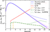 |
Fig. 1. Observed cosmic star formation rate density evolution from Shuntov et al. (2025), blue solid line and from the GLIMPSE survey at z > 9 (Chemerynska et al. 2026, blue dotted line, after conversion to the Chabrier IMF), and predicted GC formation rate, ρGC, as a function of redshift (dash-dotted and green dotted lines). The dashed line shows the observed increase in the N-emitter fraction, fN, with redshift from Morel et al. (2025), extrapolated down to z = 2 and scaled by 1/10 for convenience. |
between z ∼ 3 (the lower limit is set by the wavelength coverage of the JWST spectra) and z ∼ 14, and currently undefined at higher redshift. We adopt a maximum fN = 0.5 (predicted at z ≳ 14.4), and assume that the fraction of N-emitters becomes negligible at z < zmin ∼ 2 − 3. To back up this assumption, we examined other datasets at z ∼ 2 − 5 and z ∼ 0 − 0.4 to provide constraints on the N-emitter fraction at lower redshift, as described in the Appendix.
If fN tracks the fraction of N-emitters among star-forming galaxies as a function of redshift, the cosmic star formation rate density, ρSFR, allows us to predict–with the above assumption–the GC formation rate, ρGC; more precisely, it allows us to predict the stellar mass being formed in GCs per unit time and cosmic volume as
 (2)
(2)
where we assume ϵGC ∼ 1 (see Sect. 3.2). The result is shown in Fig. 1, where we have adopted the recent determination of ρSFR from Shuntov et al. (2025), which includes recent measurements from JWST at high redshift, and extends down to z ∼ 0. Since the N-emitter fraction and ρSFR both show a strong but opposite dependence on redshift, the product of the two depends relatively weakly on redshift, thus predicting an increase in ρGC by a factor of ∼3 from z ∼ 16 to z ∼ 3 − 4, whereas ρSFR increases by nearly three orders of magnitude over the same time.
To examine the impact of uncertainties on ρSFR at high-z, we also adopt the recent result from the GLIMPSE survey, which exploits strong gravitational lensing to determine the UV luminosity function to larger depths for galaxies above z ≳ 9 (Chemerynska et al. 2026). While these observations agree with the compilation of Shuntov et al. (2025) at z ∼ 9, they indicate a slower decrease in the star formation rate density towards higher redshifts. Since at z ≳ 10 the N-emitter fraction increases rapidly above fN > 0.1, the predicted value of ρGC could increase at these high redshifts, reaching values of ρGC(z = 16), a factor of ∼5 higher than for the more rapidly declining ρSFR history. Although ρGC depends on the product of fN × ρSFR, in which both quantities have higher uncertainties at high redshift (see Figs. 1 and A.1), this has a negligible impact on the predicted age distribution of GCs and the total mass formed in GCs, which we now discuss.
2.2. Predicted age distribution of GCs
The GC formation rate ρGC(z) can be directly translated to the predicted age distribution of GCs if we assume that the mass function of GCs at their formation is constant, on average, with cosmic time. The resulting age distribution, predicted for different lower redshift limits zmin of the occurrence of N-emitters is shown in Fig. 2. In all cases the predicted distributions are asymmetric, showing a peak age for GC formation of ∼12 − 12.5 Gyr, a rapid decrease towards older ages, and a more extended tail down to an age given by the adopted redshift cutoff age (given by zmin).
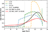 |
Fig. 2. Predicted and observed age distribution of GCs. The observational data for GCs from the Milky Way, from Kruijssen et al. (2019), and for the massive elliptical galaxy NGC 1407, from Usher et al. (2019) and compiled by Valenzuela et al. (2024), are shown as solid lines. The dash-dotted lines show the predicted age distributions from our simple model, adopting the cosmic SFR density history from Shuntov et al. (2025) for different values of zmin = 1.5, 2, and 3. The dotted line shows the same zmin = 2 and the higher ρSFR(z) values inferred from the GLIMPSE survey. |
In our simple picture, the peak age is determined by the combination of a decreasing frequency of N-emitters and the rise of cosmic SFR density, the rapid decrease at ages ≳12.5 Gyr (above the peak) is due to the decrease in ρSFR at z ≳ 8, and the tail at low ages depends on the behaviour of fN at z < 3, which is currently not constrained. In the case of a slower decrease in the cosmic star formation rate density, as suggested by the GLIMPSE survey, our simple model predicts an additional sharp peak in the age distribution of GCs at very early ages (∼13.2 Gyr, see Fig. 2). Given the typical observational age uncertainties2, this narrow peak at high-z would probably remain undetected. This also shows that the exact value of the N-emitter fraction at z ≳ 7 is not important for the predicted age distribution and that a possible contribution of active galactic nuclei (AGN) to the N-emitter population at high-z does not significantly affect this result. We discuss this issue further in Sect. 3.2.
Observed age distributions of GC populations in the Milky Way and a massive elliptical galaxy NGC 1407 are also shown in Fig. 2, for comparison. They illustrate variations of inferred age distributions in different galaxy types (see e.g. discussions in Valenzuela et al. 2024). Qualitatively, our predicted age distributions resemble the observed distributions in all three features described above, with a peak at 12–12.5 Gyr, a tail at younger ages, and a drop towards the cosmic age. Compared to other existing GC formation and evolution models, including semi-analytical, cosmological hydro, and other models, our simple models fares quite well, as can be seen from the comparison presented by Valenzuela et al. (2025).
2.3. Predicted cosmic GC mass density
Another interesting aspect of our model is that it can predict the total mass in GCs formed across cosmic time, a key quantity that can be compared to the census of GC populations in galaxies. To do so, we integrated the GC star formation rate density, ρGC, over time and plot in Fig. 3 the resulting cumulative stellar mass density hosted in GC as a function of redshift. This is compared to the classical (cumulative) stellar mass density, ρ★, derived from the integration of the adopted ρSFR from Shuntov et al. (2025) with an adopted constant return fraction R = 0.41 (Madau & Dickinson 2014). At z ≈ 0 the total stellar mass density reaches ρ★(z = 0)≈2 × 10⁸ M⊙ Mpc−3, and our predicted mass density in globulars, ρ★(GC, z = 0) = (2 − 4)×105 M⊙ Mpc−3, for 2 ≤ zmin ≤ 3.
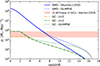 |
Fig. 3. Predicted cumulative stellar mass density evolution (SMD) in stars, ρ★, and globular clusters, ρ★(GC), as a function of redshift. The SMDs are derived from the star formation and globular cluster formation rate densities, ρSFR and ρGC, respectively, shown in Fig. 1. The shaded area indicates the range between (1 − 4) times the observed cosmic stellar mass density in GCs derived at z ∼ 0 by Harris et al. (2013), to account for the higher initial masses of GCs. |
Observationally, numerous studies have shown strong correlations between the mass of a galaxy’s GC population and the mass of its host dark matter halo or the dynamical mass of the galaxy, across many orders of magnitude in halo or galaxy mass and for different galaxy types and environments (see e.g. the review of Kruijssen 2026). Harris et al. (2013) have, for example, determined the specific mass, SM, of the GC population with respect to the baryonic mass of its host galaxy, finding a well-defined ratio of SM ≈ 0.1 per cent. This implies, observationally, a cosmological average at z ∼ 0 of the GC mass density, ρ★(GC)≈10−3 × ρ★(z = 0)≈2 × 10⁵ M⊙ Mpc−3, which closely matches our predictions, as shown in Fig. 3.
Since GCs were more massive at birth, the observed present-day mass density in GCs, ρ★(GC, z = 0), has to be corrected upwards before comparison with our prediction. Various approaches indicate that typical GCs were a factor of ∼2 − 4 more massive at birth than they are today (e.g. Reina-Campos et al. 2018; Baumgardt et al. 2019). The shaded area in Fig. 3 illustrates the range between (1 − 4)×ρ★(GC, z = 0), showing that the predicted stellar mass density of GCs (at formation) is in excellent agreement with the observations in the present-day Universe.
Figure 3 also shows that the differences between the two scenarios of the cosmic SFR evolution at high-z (z > 8) discussed above have, as expected, no significant impact on the cumulative stellar mass densities at z ≲ 4 and down to present day (z = 0), since it concerns only a short fraction of cosmic time. For the same reason, uncertainties in fN at z ≳ 8 – due to small number statistics, contamination by AGN, or other similar factors – have a negligible effect on the present-day stellar mass density in GCs.
3. Discussion
As we have just shown, the hypothesis that N-emitters trace galaxies where the UV emission is dominated by young globular clusters in formation and that their fraction follows the observed redshift dependence identified by Morel et al. (2025) leads to straightforward predictions of the average age distribution of GCs (Fig. 2) and the cosmic mass density of globulars at present times (redshift z = 0; see Fig. 3). Strikingly, these predictions are in very good agreement with the observations, despite the simplicity of our assumptions. To the best of our knowledge, this is the first empirical model reproducing the average and distribution of the formation redshifts (or ages, equivalently) of globulars, and the total baryonic mass locked up in GCs at the present day. The success of this simple model supports the idea that N-emitters could trace globular clusters, as suggested earlier, and as we now briefly discuss.
3.1. Overall picture linking N-emitters and GCs
The connection between N-emitters and GCs was first suggested based on the resemblance of the ISM abundances of N-emitters (super-solar N/O ratios and normal C/O at low metallicities) with GC stars (Charbonnel et al. 2023; Senchyna et al. 2024; Marques-Chaves et al. 2024), which are unique in showing such abundance patterns and star-to-star abundance variations (e.g. Bastian & Lardo 2018). Furthermore, the compactness of N-emitters, high ISM densities (ne ∼ 104 − 5 cm−3), high mass, and high SFR surface densities indicate unusual and extreme conditions compared to other galaxies at the same redshift (see e.g. Marques-Chaves et al. 2024; Schaerer et al. 2024; Topping et al. 2024; Arellano-Córdova et al. 2025). This is consistent with the ample evidence showing that GCs are only formed in rare high-pressure environments with a high SFR surface density, and primarily at high redshifts (Krause et al. 2020; Kruijssen 2025). In addition, the abundance variations and multiple populations found in globulars, exist only above some minimum mass (M ≳ 104 M⊙) and compactness (e.g. Krause et al. 2016), showing the existence of a threshold for their formation (Bragaglia et al. 2017; Gieles et al. 2018). In short, the available observations suggest that N-emitters and the environments where GCs are expected to form have all of these features or properties in common.
The extreme conditions found in N-emitters explain why these objects are relatively rare (less than 1% at z ≲ 5.4). Furthermore the increasing compactness of galaxies, and their increasing SFR surface density and ISM density with increasing redshift also naturally explain the observed increase in the N-emitter fraction with z, as already pointed out by Morel et al. (2025). Finally, the existence of a threshold suggests that GC formation naturally stops or becomes more rare in a Universe where the ISM conditions evolve. This is compatible with the extreme paucity of N-emitters at low redshift (see e.g. discussions in Ji et al. 2026; Martinez et al. 2025), which is described for simplicity by our adopted minimum redshift for N-emitters, zmin (see Sect. 2.1). In Appendix B we estimate the upper limit of the N-emitter fraction at low redshift from a large sample of SDSS spectra.
Our simple calculations have demonstrated quantitatively that the hypothesis that N-emitters trace the formation of GCs is compatible with the observed age distribution and the total amount of stars formed in the GC population. This provides further support to the association of N-emitters as signposts of GC formation.
3.2. Caveats and open questions
We now discuss several caveats, uncertainties, and open questions related to the predictions presented here and their interpretation.
3.2.1. Uncertainties on the N-emitter fraction and implications
The full uncertainty on the N-emitter fraction is not possible to establish. There are multiple reasons for this, including the classification of a galaxy as N-emitter (defined by the presence of one of the N IV] λ1486 and N III] λ1750 lines), which depends on the detectability of these lines, and hence on the quality of the spectra (e.g. depth, spectral resolution, width of the lines). This is not uniform in the parent sample drawn from 8323 unique sources in the DAWN JWST Archive (DJA)3 (Brammer 2023; Heintz et al. 2025). Interestingly, our determination of fN from the independent VANDELS dataset of VLT spectra of star-forming galaxies yields consistent values of fN between z ∼ 3 − 5, and also confirms the redshift increase in fN (see Appendix 4), thus supporting the empirical dependence of fN(z) from Morel et al. (2025).
Should fN be systematically higher at all redshifts, for example by a factor of 2, as the current data may allow, this would obviously not alter the predicted GC age distribution and would simply increase ρGC and the cumulative stellar mass density in GCs at all redshifts, ρ★(GC), by the same amount. Such an increase can easily be compensated by lowering the GC formation efficiency, ϵGC, which we discuss below. Lower fractions of fN are very unlikely since the N-emitter sample should be quite robust and since the total number of star-forming galaxies plus AGN is quite easily established from the parent sample, with less uncertainty than the identification of nitrogen lines.
Given the different object selections and methods used to determine N/O abundance ratios discussed in the literature, one may wonder how well fN used here accounts for all objects with a high N/O abundance, or whether our selection misses some objects. As mentioned earlier, our UV selection (presence of N IV] λ1486 or N III] λ1750) roughly translates to a super-solar N/O ratio (log(N/O)≳ − 0.8). Several galaxies with super-solar N/O ratios reported in the literature (e.g. Sanders et al. 2023; Stiavelli et al. 2025) are not included in the sample of Morel et al. (2025). For these objects the abundances have been derived from optical medium-resolution spectra including [N II] λλ6584, but rest-UV spectra (including PRISM spectra) are currently not available. However, since the number of medium-resolution spectra required to determine the N-abundance from optical spectra ([N II] λλ6584) is currently small, statistical studies are not yet possible with these data, in contrast to the large number of PRISM spectra available. Finally, for a small number of objects it has been possible to determine N/O with several methods, using separately UV and optical lines. In general a good or reasonable agreement between the UV and optical methods has been found (e.g. Berg et al. 2025; Moreschini et al. 2026; Welch et al. 2025; Marques-Chaves et al. 2024), indicating that the UV-selection of N-emitters adopted by Morel et al. (2025) should (on average) not miss objects with similarly high N/O ratios determined from optical spectra.
Finally, the question arises of whether the simple measure of the N-emitter fraction misses some GCs in formation, for example systems, if they exist, that are not enhanced in nitrogen or are insignificantly enhanced. For several decades GCs have been shown to systematically exhibit peculiar features (compared to other star clusters), which include the presence of multiple stellar populations and star-to-star variations of specific elements (N, O, Na, Al, and others) and are now the defining characteristics of globulars (see e.g. reviews of Gratton et al. 2004; Bastian & Lardo 2018). By definition, every GC therefore contains N-enriched stars (compared to their initial N-abundance), although with varying degrees of N-enrichment and varying fractions of stars being enriched. For GCs with masses between 104 and 106 M⊙, for example, the fraction of enriched stars varies from ∼0.4 to 0.8 (Bastian & Lardo 2018) and [N/Fe] increases by up to ∼1.3 dex (e.g. Carlos et al. 2023). To summarise, at the time of formation of the enriched stars, all GCs must have had some N-enriched gas. However, how this relates with the enrichment seen in the ionised ISM cannot be quantified. In practice this means that our method could miss some GCs, a case already discussed above.
3.2.2. Contamination by AGN
Despite the various and new arguments in favour of a link between N-emitters and young globular clusters, the nature of N-emitters is still debated. Zhu et al. (2026) have recently studied eight N-emitters at z ∼ 6 − 11 with medium-resolution spectra from JWST and conclude that seven of them are best described by N-enhanced AGN models. The question hence arises whether our conclusions would be affected if the majority of N-emitters at z ≳ 6 − 8 were AGN. In fact, the AGN classification is also debated, as illustrated by two well-studied N-emitters where no consensus has been reached, GNz-11 and CEERS-1019 (Larson et al. 2023; Maiolino et al. 2024; Álvarez-Márquez et al. 2025; Zamora et al. 2025). In addition, most of the N-emitters studied to date, if not all, show compact but resolved morphologies (cf. Morel et al. 2025). This suggests that AGN are unlikely to be the dominant source of the UV continuum in N-emitters. Furthermore, if the fraction fN of N-emitters associated with star or GC formation were reduced at high-z, this would have a small or negligible impact on the predicted GC age distribution and the total mass formed in N-emitters, as shown above. Finally, analysing the largest N-emitter sample known to date, Morel et al. (2025) found only a small fraction of objects (4/45 ≈ 8%) with signatures of broad-line AGN, and few such objects at z ≲ 7. Further work is needed to establish the importance of AGN among N-emitters and to test the various proposed scenarios. In any case, our main results remain unchanged if the majority of N-emitters at z ≲ 7 are related to star cluster formation, not AGN.
3.2.3. High GC formation efficiency
In our calculation of the total stellar mass density in GCs, ρ★(GC), we assume that the bulk of star formation in N-emitters produces (and ends up in) globular clusters, i.e. ϵGC ∼ 1, which is probably a somewhat optimistic assumption. This basically postulates a high cluster formation efficiency (CFE) and a cluster mass distribution with a minimum cluster mass close to or above the threshold for the formation of GC (∼104 M⊙), in other words, a small amount of mass in low-mass clusters that cannot become globulars.
Whereas high CFE ∼0.5 − 1 are commonly observed in the high-z Universe and in high SFR surface density galaxies (e.g. Adamo et al. 2020), the mass function of stellar clumps or clusters is currently not yet constrained at masses below ∼105 M⊙ (Claeyssens et al. 2025). One case of a high-z galaxy showing a CFE near unity and a cluster mass function leaving no room for low-mass clusters has recently been found by Vanzella et al. (2026); it has been given the nickname of Cosmic Gems galaxy. Whether this is a common property remains to be explored in the future. Although maximal, these assumptions are not incompatible with current observations, and it should be remembered that they only need to apply to rare objects (N-emitters), which already show other properties that are extreme (see above).
We also note that the N-emitter fraction adopted might be underestimated, since it relies on the detection of UV emission lines, which is biased towards strong N lines (Zhu et al. 2025). This, or other cases leading to an underestimate of fN, would allow us to relax the assumption of ϵGC ∼ 1 and maintain a total stellar mass density in GCs compatible with observations at z ∼ 0. Physically, values of ϵGC < 1 are easy to explain, for example as being due to the formation of clusters below the mass limit of GCs or to the evaporation or tidal destruction of globulars (see e.g. references in Kruijssen 2025).
Future investigations will be necessary to firm up or disprove the suggested link between N-emitters and proto-GCs, to which our approach adds a new statistical aspect on their populations.
4. Conclusions
It has been proposed that N-emitters, i.e. strongly N-enhanced galaxies with uncommon UV emission lines of nitrogen revealed by JWST observations, could be related to young globular clusters (GCs) forming in situ (Charbonnel et al. 2023; Senchyna et al. 2024). To test this hypothesis we used the recently determined frequency of N-emitters and their observed redshift evolution from Morel et al. (2025) to compute the cosmological average of the GC star formation rate density, ρGC; the resulting age distribution of globulars; and–to the best of our knowledge, for the first time–the cumulative stellar mass density in GCs across cosmic times, from the observed cosmic star formation history ρSFR(z).
We find that GC formation is predicted to peak at z ∼ 3 − 4 (ages ∼11.5 − 12 Gyr), with an asymmetric age distribution showing an extended tail to younger ages and a rapid drop beyond ≳12.5 Gyr, independently of the exact values of ρSFR at very high redshifts, where it is currently being determined. The predicted GC age distribution resembles the typical distribution of GCs in the Milky Way and in elliptical galaxies.
The predicted total stellar mass density formed in N-emitters down to redshift zero, ρ★(GC, z = 0) = (2 − 4)×105 M⊙ Mpc−3, matches within a factor of ∼2 the observed fraction of stellar mass found in the GC population at z = 0 ( = 10−3 of the total stellar mass density of galaxies, Harris et al. 2013). Our results provide additional support to the hypothesis that N-emitters represent signposts of GC formation, and that these phenomena are thus related.
Acknowledgments
DS wishes to thank the IAP, Paris, and its staff for their hospitality during a stay where some of this work was done. We also thank Lucas Valenzuela for sharing results in electronic format. YI and NG acknowledge support from the National Academy of Sciences of Ukraine (Project No. 0126U000353).
References
- Adamo, A., Hollyhead, K., Messa, M., et al. 2020, MNRAS, 499, 3267 [Google Scholar]
- Adamo, A., Bradley, L. D., Vanzella, E., et al. 2024, Nature, 632, 513 [NASA ADS] [CrossRef] [Google Scholar]
- Álvarez-Márquez, J., Crespo Gómez, A., Colina, L., et al. 2025, A&A, 695, A250 [NASA ADS] [CrossRef] [EDP Sciences] [Google Scholar]
- Arellano-Córdova, K. Z., Berg, D. A., Mingozzi, M., et al. 2025, MNRAS, 544, 1588 [Google Scholar]
- Asplund, M., Grevesse, N., Sauval, A. J., & Scott, P. 2009, ARA&A, 47, 481 [NASA ADS] [CrossRef] [Google Scholar]
- Barchiesi, L., Dessauges-Zavadsky, M., Vignali, C., et al. 2023, A&A, 675, A30 [NASA ADS] [CrossRef] [EDP Sciences] [Google Scholar]
- Bastian, N., & Lardo, C. 2018, ARA&A, 56, 83 [Google Scholar]
- Baumgardt, H., Hilker, M., Sollima, A., & Bellini, A. 2019, MNRAS, 482, 5138 [Google Scholar]
- Berg, D. A., James, B. L., King, T., et al. 2022, ApJS, 261, 31 [NASA ADS] [CrossRef] [Google Scholar]
- Berg, D. A., Naidu, R. P., Chisholm, J., et al. 2025, arXiv e-prints [arXiv:2511.13591] [Google Scholar]
- Bhattacharya, S., & Kobayashi, C. 2025, arXiv e-prints [arXiv:2508.11998] [Google Scholar]
- Borghi, N., Moresco, M., Cimatti, A., et al. 2022, ApJ, 927, 164 [NASA ADS] [CrossRef] [Google Scholar]
- Bragaglia, A., Carretta, E., D’Orazi, V., et al. 2017, A&A, 607, A44 [NASA ADS] [CrossRef] [EDP Sciences] [Google Scholar]
- Brammer, G. 2023, https://doi.org/10.5281/zenodo.7299500 [Google Scholar]
- Bunker, A. J., Saxena, A., Cameron, A. J., et al. 2023, A&A, 677, A88 [NASA ADS] [CrossRef] [EDP Sciences] [Google Scholar]
- Carlos, M., Marino, A. F., Milone, A. P., et al. 2023, MNRAS, 519, 1695 [Google Scholar]
- Cataldi, E., Belfiore, F., Curti, M., et al. 2025, A&A, submitted [arXiv:2512.07955] [Google Scholar]
- Chabrier, G. 2003, PASP, 115, 763 [Google Scholar]
- Charbonnel, C., Schaerer, D., Prantzos, N., et al. 2023, A&A, 673, L7 [NASA ADS] [CrossRef] [EDP Sciences] [Google Scholar]
- Chemerynska, I., Atek, H., Furtak, L. J., et al. 2026, MNRAS, 546, staf2267 [Google Scholar]
- Claeyssens, A., Adamo, A., Messa, M., et al. 2025, MNRAS, 537, 2535 [Google Scholar]
- Garilli, B., McLure, R., Pentericci, L., et al. 2021, A&A, 647, A150 [NASA ADS] [CrossRef] [EDP Sciences] [Google Scholar]
- Gieles, M., Charbonnel, C., Krause, M. G. H., et al. 2018, MNRAS, 478, 2461 [Google Scholar]
- Gratton, R., Sneden, C., & Carretta, E. 2004, ARA&A, 42, 385 [Google Scholar]
- Harris, W. E., Harris, G. L. H., & Alessi, M. 2013, ApJ, 772, 82 [Google Scholar]
- Heintz, K. E., Brammer, G. B., Watson, D., et al. 2025, A&A, 693, A60 [Google Scholar]
- Izotov, Y. I., Thuan, T. X., & Lipovetsky, V. A. 1994, ApJ, 435, 647 [NASA ADS] [CrossRef] [Google Scholar]
- Izotov, Y. I., Guseva, N. G., Fricke, K. J., et al. 2021, A&A, 646, A138 [NASA ADS] [CrossRef] [EDP Sciences] [Google Scholar]
- James, B. L., Tsamis, Y. G., Barlow, M. J., et al. 2009, MNRAS, 398, 2 [Google Scholar]
- Ji, X., Belokurov, V., Maiolino, R., et al. 2026, MNRAS, 545, staf2110 [Google Scholar]
- Krause, M. G. H., Charbonnel, C., Bastian, N., & Diehl, R. 2016, A&A, 587, A53 [NASA ADS] [CrossRef] [EDP Sciences] [Google Scholar]
- Krause, M. G. H., Offner, S. S. R., Charbonnel, C., et al. 2020, Space Sci. Rev., 216, 64 [CrossRef] [Google Scholar]
- Kruijssen, J. M. D. 2025, arXiv e-prints [arXiv:2501.16438] [Google Scholar]
- Kruijssen, J. M. D. 2026, Encyclopedia of Astrophysics, 4, 500 [Google Scholar]
- Kruijssen, J. M. D., Pfeffer, J. L., Reina-Campos, M., Crain, R. A., & Bastian, N. 2019, MNRAS, 486, 3180 [Google Scholar]
- Larson, R. L., Finkelstein, S. L., Kocevski, D. D., et al. 2023, ApJ, 953, L29 [NASA ADS] [CrossRef] [Google Scholar]
- Madau, P., & Dickinson, M. 2014, ARA&A, 52, 415 [Google Scholar]
- Maiolino, R., Scholtz, J., Witstok, J., et al. 2024, Nature, 627, 59 [NASA ADS] [CrossRef] [Google Scholar]
- Marques-Chaves, R., Schaerer, D., Kuruvanthodi, A., et al. 2024, A&A, 681, A30 [NASA ADS] [CrossRef] [EDP Sciences] [Google Scholar]
- Martinez, Z., Berg, D. A., James, B. L., et al. 2025, ApJ, 995, 204 [Google Scholar]
- Morel, I., Schaerer, D., Marques-Chaves, R., et al. 2025, A&A, submitted [arXiv:2511.20484] [Google Scholar]
- Moreschini, B., Belfiore, F., Marconi, A., et al. 2026, arXiv e-prints [arXiv:2601.08939] [Google Scholar]
- Pustilnik, S., Kniazev, A., Pramskij, A., et al. 2004, A&A, 419, 469 [NASA ADS] [CrossRef] [EDP Sciences] [Google Scholar]
- Reina-Campos, M., Kruijssen, J. M. D., Pfeffer, J., Bastian, N., & Crain, R. A. 2018, MNRAS, 481, 2851 [NASA ADS] [CrossRef] [Google Scholar]
- Sanders, R. L., Shapley, A. E., Clarke, L., et al. 2023, ApJ, 943, 75 [Google Scholar]
- Schaerer, D., Marques-Chaves, R., Xiao, M., & Korber, D. 2024, A&A, 687, L11 [NASA ADS] [CrossRef] [EDP Sciences] [Google Scholar]
- Schreiber, C., Glazebrook, K., Nanayakkara, T., et al. 2018, A&A, 618, A85 [NASA ADS] [CrossRef] [EDP Sciences] [Google Scholar]
- Senchyna, P., Plat, A., Stark, D. P., et al. 2024, ApJ, 966, 92 [NASA ADS] [CrossRef] [Google Scholar]
- Shuntov, M., Ilbert, O., Toft, S., et al. 2025, A&A, 695, A20 [NASA ADS] [CrossRef] [EDP Sciences] [Google Scholar]
- Stiavelli, M., Morishita, T., Chiaberge, M., et al. 2025, ApJ, 981, 136 [Google Scholar]
- Talia, M., Schreiber, C., Garilli, B., et al. 2023, A&A, 678, A25 [NASA ADS] [CrossRef] [EDP Sciences] [Google Scholar]
- Thuan, T. X., Izotov, Y. I., & Lipovetsky, V. A. 1996, ApJ, 463, 120 [NASA ADS] [CrossRef] [Google Scholar]
- Topping, M. W., Stark, D. P., Senchyna, P., et al. 2024, MNRAS, 529, 3301 [NASA ADS] [CrossRef] [Google Scholar]
- Usher, C., Brodie, J. P., Forbes, D. A., et al. 2019, MNRAS, 490, 491 [NASA ADS] [CrossRef] [Google Scholar]
- Valenzuela, L. M., Remus, R.-S., McKenzie, M., & Forbes, D. A. 2024, A&A, 687, A104 [NASA ADS] [CrossRef] [EDP Sciences] [Google Scholar]
- Valenzuela, L. M., Forbes, D. A., & Remus, R.-S. 2025, MNRAS, 537, 306 [CrossRef] [Google Scholar]
- Vanzella, E., Calura, F., Meneghetti, M., et al. 2017, MNRAS, 467, 4304 [Google Scholar]
- Vanzella, E., Calura, F., Meneghetti, M., et al. 2019, MNRAS, 483, 3618 [Google Scholar]
- Vanzella, E., Claeyssens, A., Welch, B., et al. 2023, ApJ, 945, 53 [NASA ADS] [CrossRef] [Google Scholar]
- Vanzella, E., Messa, M., Adamo, A., et al. 2026, A&A, 705, A171 [NASA ADS] [CrossRef] [EDP Sciences] [Google Scholar]
- Vila-Costas, M. B., & Edmunds, M. G. 1993, MNRAS, 265, 199 [NASA ADS] [CrossRef] [Google Scholar]
- Welch, B., Rivera-Thorsen, T. E., Rigby, J. R., et al. 2025, ApJ, 980, 33 [Google Scholar]
- Zamora, S., Carniani, S., Bertola, E., et al. 2025, A&A, submitted [arXiv:2512.09022] [Google Scholar]
- Zhu, P., Kewley, L. J., Hsiao, T. Y.-Y., & Trussler, J. 2025, ApJ, 994, L29 [Google Scholar]
- Zhu, P., Trussler, J., & Kewley, L. J. 2026, ApJ, 998, 5 [Google Scholar]
The solar ratio is log(N/O) = − 0.86, according to Asplund et al. (2009).
For example, in the MW GC data used here from the compilation of Valenzuela et al. (2025) the mean age uncertainty is 0.55 Gyr.
This follows the methods from Schreiber et al. (2018) and Borghi et al. (2022).
Appendix A: New constraints on the N-emitter fraction at z ∼ 2 − 5 from VANDELS
To complement and possibly extend the recent statistics of N-emitters derived from JWST spectra to lower redshifts, we have examined the data from VANDELS, a deep, uniform, spectroscopic galaxy survey undertaken with the VIMOS instrument at the VLT. To do so, we have used the spectra from the latest data release (Garilli et al. 2021) and, following Talia et al. (2023), we have extended the catalog of spectroscopic measurements to include the N III] λ1750 and N IV] λλ 1483,1486 features. This is done with Gaussian fits and direct integrations adapted to the doublet or multiplet structure of these line complexes.4
Eliminating passive galaxies from the full sample, following the UVJ selection described in Garilli et al. (2021), we are left with 1501 galaxies in the redshift interval 1.75 ≲ z ≲ 5.75, where N III] λ1750 or N IV] λλ 1483,1486 can in principle be detected. Our automated measurement yields ∼10 candidates at ≳3 − 4σ, including the well-known N-emitter VANDELS_CDFS_003073, an AGN at z = 5.56 (see Barchiesi et al. 2023; Ji et al. 2026, and references therein). After visual inspection, only one additional object with a credible N III] λ1750 detection, VANDELS_CDFS_247555 at z = 3.745 remains, yielding thus a total detection fraction of N-emitters of 1.3 × 10⁻³ among the VANDELS star-forming galaxies and AGN showing rest-UV emission.
From these detections and non-detections we derive the fraction of N-emitters in several redshift bins between 1.75 ≲ z ≲ 5.75, computing the confidence intervals with the Wilson interval formula, which is adapted for small sample sizes and low fractions. The result is plotted in Fig. A.1 together with the N-emitter fraction determined by Morel et al. (2025) from archival JWST NIRSpec PRISM data including large samples. Clearly, the VANDELS and JWST data are consistent with the reported redshift evolution of fN (Eq. 1). Furthermore, the VANDELS data is compatible with a low fraction at z ∼ 2 − 3, although the statistical uncertainties are relatively large. The new data thus supports the adopted description of fN(z) and drop at zmin ∼ 2 − 3.
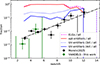 |
Fig. A.1. Redshift evolution of the fraction of N-emitters (circles) as a function of redshift, determined by Morel et al. (2025) from the JWST NIRSpec PRISM spectra (black circles and limits) and from the VANDELS survey (green circles and limits). The uncertainties show the 68% confidence range of the fractions, and the bin width along the x-axis. The blue lines show the fraction of rest-UV line emitters 4σ (solid) or 3σ detection (dotted) thresholds. The fraction of objects showing rest-optical emission lines is shown by the red line, and all emission-line galaxies (UV and/or optical) in magenta (dashed). The black dash-dotted line shows the fit to the z > 3 data, Eq. 1, obtained by Morel et al. (2025). |
Finally, we note that the fN values obtained from the JWST and the VANDELS data agree approximately, despite the different properties (e.g. spectral resolution, average S/N) of the data. While the typical threshold (3 σ upper limits) for the N III] λ1750 and N IV] λ1486 lines is ∼10 Å in the JWST PRISM spectra (see Morel et al. 2025), the median 3-σ limit is ∼6 Å in the VANDELS spectra, i.e. somewhat but not significantly lower.
Appendix B: N-emitter fraction at low redshift
To the best of our knowledge, no systematic search for the N IV] λ1486 and N III] λ1750 lines has so far been undertaken in galaxy spectra at low-z, and the current compilations of galaxies with UV spectroscopy from the Hubble Space telescope (HST) and earlier, are small (see e.g. Berg et al. 2022, who cite other compilations, including in total 270 galaxies). Focussing on 46 high-quality HST spectra primarily from the CLASSY survey (Berg et al. 2022), Martinez et al. (2025) have recently identified up to eight galaxies with clear or possible nitrogen emission lines, including the well-studied WR-galaxy Mrk 996 (J0127-06719), which was previously reported as a clear N-emitter at low-z (Thuan et al. 1996). From their abundance determinations using UV and optical emission lines, Martinez et al. (2025) find only one object (Mrk 996) with a robust super-solar N/O ratio.
Mrk 996 has long been known as a blue compact dwarf galaxy (BCD) with very peculiar properties, showing a very compact nucleus, broad emission lines, WR features, very high electron densities in the nucleus, and other unusual properties (e.g. Izotov et al. 1994; Thuan et al. 1996). Furthermore, it was found among a small group of BCDs with a significant overabundance of N/O compared to other galaxies and BCDs at similar metallicities (O/H; see e.g. Pustilnik et al. 2004; James et al. 2009).
Larger samples including the SDSS, have not found significant numbers of objects with high N/O abundances, comparable to those of the high-z N-emitters. To quantify this, we have used the spectroscopic sample of ∼25000 compact star-forming galaxies constructed by Izotov et al. (2021) who have used SDSS spectra. Among those, 2212 objects have a significant [O III]λ4363 detection, allowing for O/H measurements using the direct method. For this sub-sample we then determined the N/O abundance ratio from the [N II] λλ6584/[O II] λ3727 ratio, using the recent calibration from Cataldi et al. (2025). The result is illustrated in Fig. B.1. We find a mean N/O ratio of  , and a slight dependence of N/O with O/H, as well known from the literature. Most importantly, very few or no objects are found at the high N/O ratios found in N-emitters log(N/O)≳ − 0.8, which translates to an upper limit of ≲4.5 × 10⁻⁴ for the fraction of these objects among the sample of galaxies with accurate O/H at z ≲ 0.4.
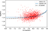 |
Fig. B.1. N/O abundance ratio as a function of O/H from the sample of 2212 low-z compact star-forming galaxies from Izotov et al. (2021) with [O III]λ4363 detections. N/O was determined from the [N II] λλ6584/[O II] λ3727 ratio using the recent calibration from Cataldi et al. (2025) for low-z galaxies. The solid line shows their mean relation at low-z, the dash-dotted line that from Vila-Costas & Edmunds (1993). The figure illustrates the absence of low-z objects with very high N/O abundances ( |
For comparison, Bhattacharya & Kobayashi (2025) recently determined the N/O abundances for a sample of 944 star-forming galaxies with direct abundance determinations using spectra from the Dark Energy Spectroscopic Instrument (DESI). Among those, they report the finding of 19 galaxies with log(N/O)≥ − 1.1, which they denote as extreme N-emitters, and four objects with super-solar N/O ratios at 12 + log(O/H) < 7.5. Inspection of the spectra of these four objects shows that the [O III]λ4363 line is not securely detected and/or that their oxygen abundances are unlikely to be very low since most of these objects have relatively high stellar masses, including one large spiral galaxy (their Fig. 4), which appears at odds with the very low metallicities reported for these systems. From this we conclude that their sample is compatible with the above analysis of the larger SDSS sample, and that essentially none of these galaxies show N/O abundance ratios comparable to the N-emitters, as defined in this work. Assuming that the N/O abundance ratios determined from optical lines ([N II] λλ6584 and [O II] λ3727) agree on average with those from the UV lines and that N-emitters have typically log(N/O)≳ − 0.8, we therefore estimate an upper limit of the N-emitter fraction of fN(z ∼ 0 − 0.4)≲4.5 × 10⁻⁴ at low-z, from the currently largest datasets available. This limit supports our assumption of a rapid drop of fN at z ≲ 2.
All Figures
|
Fig. 1. Observed cosmic star formation rate density evolution from Shuntov et al. (2025), blue solid line and from the GLIMPSE survey at z > 9 (Chemerynska et al. 2026, blue dotted line, after conversion to the Chabrier IMF), and predicted GC formation rate, ρGC, as a function of redshift (dash-dotted and green dotted lines). The dashed line shows the observed increase in the N-emitter fraction, fN, with redshift from Morel et al. (2025), extrapolated down to z = 2 and scaled by 1/10 for convenience. |
| In the text | |
|
Fig. 2. Predicted and observed age distribution of GCs. The observational data for GCs from the Milky Way, from Kruijssen et al. (2019), and for the massive elliptical galaxy NGC 1407, from Usher et al. (2019) and compiled by Valenzuela et al. (2024), are shown as solid lines. The dash-dotted lines show the predicted age distributions from our simple model, adopting the cosmic SFR density history from Shuntov et al. (2025) for different values of zmin = 1.5, 2, and 3. The dotted line shows the same zmin = 2 and the higher ρSFR(z) values inferred from the GLIMPSE survey. |
| In the text | |
|
Fig. 3. Predicted cumulative stellar mass density evolution (SMD) in stars, ρ★, and globular clusters, ρ★(GC), as a function of redshift. The SMDs are derived from the star formation and globular cluster formation rate densities, ρSFR and ρGC, respectively, shown in Fig. 1. The shaded area indicates the range between (1 − 4) times the observed cosmic stellar mass density in GCs derived at z ∼ 0 by Harris et al. (2013), to account for the higher initial masses of GCs. |
| In the text | |
|
Fig. A.1. Redshift evolution of the fraction of N-emitters (circles) as a function of redshift, determined by Morel et al. (2025) from the JWST NIRSpec PRISM spectra (black circles and limits) and from the VANDELS survey (green circles and limits). The uncertainties show the 68% confidence range of the fractions, and the bin width along the x-axis. The blue lines show the fraction of rest-UV line emitters 4σ (solid) or 3σ detection (dotted) thresholds. The fraction of objects showing rest-optical emission lines is shown by the red line, and all emission-line galaxies (UV and/or optical) in magenta (dashed). The black dash-dotted line shows the fit to the z > 3 data, Eq. 1, obtained by Morel et al. (2025). |
| In the text | |
|
Fig. B.1. N/O abundance ratio as a function of O/H from the sample of 2212 low-z compact star-forming galaxies from Izotov et al. (2021) with [O III]λ4363 detections. N/O was determined from the [N II] λλ6584/[O II] λ3727 ratio using the recent calibration from Cataldi et al. (2025) for low-z galaxies. The solid line shows their mean relation at low-z, the dash-dotted line that from Vila-Costas & Edmunds (1993). The figure illustrates the absence of low-z objects with very high N/O abundances ( |
| In the text | |
Current usage metrics show cumulative count of Article Views (full-text article views including HTML views, PDF and ePub downloads, according to the available data) and Abstracts Views on Vision4Press platform.
Data correspond to usage on the plateform after 2015. The current usage metrics is available 48-96 hours after online publication and is updated daily on week days.
Initial download of the metrics may take a while.