| Issue |
A&A
Volume 708, April 2026
|
|
|---|---|---|
| Article Number | A123 | |
| Number of page(s) | 10 | |
| Section | The Sun and the Heliosphere | |
| DOI | https://doi.org/10.1051/0004-6361/202558785 | |
| Published online | 01 April 2026 | |
Sunspot simulations with MURaM
I. Parameter study using potential field initial conditions
1
Institut für Sonnenphysik (KIS), Georges-Köhler-Allee 401a, 79110 Freiburg, Germany
2
Astronomical Institute of the Czech Academy of Sciences, Fričova 298, 25165 Ondřejov, Czech Republic
★ Corresponding author: This email address is being protected from spambots. You need JavaScript enabled to view it.
Received:
24
December
2025
Accepted:
10
February
2026
Abstract
Context. Existing sunspot simulations fail to reproduce the observed magnetic field distribution due to an artificially increased Bhor at the upper boundary.
Aims. We explore alternative ways to better reproduce the magnetic and dynamic properties of observed sunspots.
Methods. We used the MURaM radiative magnetohydrodynamic code. As the initial conditions, we placed a potential magnetic field into small-scale dynamo simulations and used potential field extrapolation as the top boundary conditions.
Results. We find that (1) simulations with increasing initial magnetic field strengths (20 kG, 40 kG, 80 kG, and 160 kG) show increasing spot, umbral, and penumbral sizes; (2) penumbral-to-spot sizes are smaller than those measured in observed sunspots; (3) none of the runs show pure Evershed (radially outwards) flows and, instead, bi-directional flows with inflows in the inner penumbra and outflows in the outer penumbra were measured, consistent with observations of early stages of penumbra formation for runs with 80 kG or more and 96/32 km resolution, whereas runs with ≤40 kG showed pure inflows; (4) simulations with 160 kG and an increased resolution of 32/16 km contain filaments with bi-directional and Evershed flows; (5) simulations with fluxes > 1022 Mx show unrealistically strong fields in the umbra; and (6) best runs with 160 kG and 1022 Mx give realistic profiles of Bz and Br with radius, albeit with stronger fields than those typically observed. Finally, (7) increasing the width of the box and reducing the overall flux by subtracting a uniform opposing vertical field have little influence on internal spot dynamics and fields. Nonetheless, these choices affect the average vertical field beyond the spot.
Conclusions. Simulations of small (1022 Mx) sunspots with an initial potential field and intensified magnetic field strength at the bottom of the box seem to best reproduce observational results of the initial stages of sunspot formation. Our findings also suggest that increased numerical resolution could be critical for achieving fully developed penumbrae.
Key words: magnetohydrodynamics (MHD) / methods: numerical / Sun: magnetic fields / Sun: photosphere / sunspots
© The Authors 2026
 Open Access article, published by EDP Sciences, under the terms of the Creative Commons Attribution License (https://creativecommons.org/licenses/by/4.0), which permits unrestricted use, distribution, and reproduction in any medium, provided the original work is properly cited.
This article is published in open access under the Subscribe to Open model. This email address is being protected from spambots. You need JavaScript enabled to view it. to support open access publication.
1. Introduction
The art of magnetohydrodynamic (MHD) sunspot simulations has only recently been developed. In 2007, Heinemann et al. (2007) presented the first slab simulation of a sunspot, followed by similar simulations by Scharmer et al. (2008) and Rempel et al. (2009b). These simulations provided the first insights into the penumbral fine structure. Following a series of initial trials, particularly in (Rempel et al. 2009a), Rempel (2012) managed to run MHD simulations of a circular sunspot that qualitatively reproduced the observed properties of penumbral fine structure. In other words, the structure of the penumbral filaments is comparable to the observational analysis of (Tiwari et al. 2013).
However, the formation of an extended penumbra has been achieved in these MHD simulations by imposing artificial top boundary conditions that make the magnetic field more horizontal at the photospheric level. As shown by (Jurčák et al. 2020), the global magnetic properties of the resulting sunspot are not fully realistic. The magnetic field inclination on the umbral-penumbral boundary is around 60°, which is significantly more horizontal than in the observed sunspots, where the highest values for the inclination are around 45° and occur only in large sunspots with more flux than the simulated sunspot. Furthermore, the vertical magnetic field component, Bz, at the umbral boundary in these simulations is below the value expected from observations, a Bzstable of around 1.8 kG. In Jurčák et al. (2020), it was also shown that the inclination distribution as a function of the fractional spot radius, as well as Bz at the umbral boundary of observed sunspots, is comparable to an MHD simulation of a sunspot with a potential field as an initial condition. The use of a potential field as an initial condition for sunspot simulations was first proposed by Nordlund (2015), using slab geometry. Based on this idea, we performed an MHD simulation of a circular sunspot, as described by Jurčák et al. (2020). To find the best agreement between the simulated and observed sunspots, we conducted a parameter study of sunspot simulations using potential field initial conditions.
The sunspot simulations of Panja et al. (2021) also adopted potential top boundary conditions. However, the penumbra of their sunspots was wide only between the nearby opposite polarity spots and very narrow in the perpendicular direction. Furthermore, their simulations are, by design, strongly affected by fluting instability, which makes them short-lived. The same authors also created simulations of starspots on other main sequence stars (Panja et al. 2020). Bhatia et al. (2025) simulated starspots, extending the work of Panja et al. (2020), but again forcing the magnetic field at the top to be inclined, resulting in too horizontal fields, at least when comparing the G2V starspot to sunspot observations.
Hideyuki Hotta investigated the effect of higher resolution on sunspot simulations with a potential-field top boundary condition. Matthias Rempel joined this investigation and also analysed what happens when the resolution is changed during the simulation runs. All simulations in their investigation use potential field top boundary conditions. While presentations of preliminary analysis (Rempel & Hotta 2025) are very encouraging, these results have not yet been published in a peer-reviewed journal. Furthermore, the high resolution used in these simulations results in prohibitively high costs.
In solar observations, the penumbra forms around existing flux concentrations (e.g. Schlichenmaier et al. 2010b). Various authors have done flux emergence simulations (e.g. Cheung et al. 2010; Chen et al. 2017; Hotta & Iijima 2020). These simulations show, consistently with solar surface observations, that deeply anchored bundles rise coherently up to around 2 Mm below the surface, to then decay in small parts that rise with individual convective cells. At the surface, they re-coalesce to larger structures that end up forming sunspots (see the ‘tethered-balloon’ model of Spruit 1981). However, they either manage to create a wide enough penumbra at most in some directions or have incorrect flow directions (inflows along the filaments and downflows at the umbral boundary) in most or all penumbral filaments.
In the following, Sect. 2 describes the simulation setups, including the initial conditions, their variables, and the values they take, as well as the data processing methods. Section 3 presents the results, focusing on intensities, surface flows, and magnetic field properties. Section 4 provides a summary and conclusion, including a discussion of how the results relate to observations.
2. Simulation set-ups and processing
Our simulations were run using the MPS/University of Chicago Radiative Magneto-hydrodynamics code (MURaM; Vögler et al. 2004; Rempel et al. 2009b). We used the updated numerical treatment from Rempel (2017), without using the coronal features introduced therein. The bottom boundary is open to mass flows and the magnetic fields are extrapolated symmetrically, as described by Rempel (2014, Sect. 2.2, item ‘OSb’). The top boundary is open to inflows and closed to outflows, with the magnetic field potential as in Cheung (2006, Appendix C.1) and Rempel (2012, Appendix B).
2.1. Initial condition: Potential with opposing flux
The initial vertical component of the magnetic field at the bottom of the box is given by
 (1)
(1)
where B0 is the initial maximal magnetic field, r is the distance from the spot axis, and FGauss is the flux contributed by the Gaussian distribution. An alternative to a pure Gaussian is the subtraction of a uniform vertical magnetic field, Bopp. Performing a horizontal integration gives the total flux through the box,
 (2)
(2)
where w is the width of the box in both the horizontal directions. This value is the same for all heights and all times (but not over the τ = 1 iso-surface). The initial field throughout the box is given by potential field extrapolation according to
 (3)
(3)
where ℱ represents the horizontal Fourier transform. By can be obtained by replacing kx by ky, or in our axisymmetric case, via By(x, y) = Bx(y, x). This extrapolation is the same as the top boundary condition mentioned above, with the difference that there z = 0 stands for the top (extrapolation into the ghost cells during the simulation run) instead of the bottom of the box (creating the initial field).
The potential extrapolation results in the initial Bz falling much more slowly with increasing radius outside the spot (see Fig. A.1, top-left panel) than self-similar initial conditions as in Rempel (2012). For all initial conditions with a pure Gaussian in the smaller simulation box, Bz remained above 155 G everywhere in the box. Given that in observations, Bz outside the spot vanishes, we tested the effect of subtracting a uniform vertical field (Bopp). This subtraction can be performed before or after extrapolation and the result is the same.
2.2. Simulation dataset
The simulation runs described in this article are listed in Table 1, where the following parameters were varied:
-
Initial maximal magnetic field strength B0: 20 kG, 40 kG, 80 kG, or 160 kG (most runs). B0 is the first number in run names.1
-
Box width, w: 49.152 Mm (most runs) or 98.304 Mm. Runs with w = 98.304 Mm have names ending in ‘w’.
-
FGauss = 1022 Mx (most runs) or Ftot = 1022 Mx. Runs with FGauss > 1022 Mx have names ending in ‘c’.
-
Opposing magnetic field Bopp: 0 G, 50 G, 100 G, 150 G, 200 G, and 300 G. This is the second number in the simulation names.
-
Most runs use a 96 (32) km horizontal (vertical) resolution, except the high-resolution runs with 32 (16) km, which have a name ending containing ‘h’. All low-resolution simulations use a grey radiative transfer.
Simulation parameters.
The simulations with names ending in ‘o’ were run with a previous version of the MURaM code and provided bolometric intensities instead of 500 nm continuum intensities. They also contain further subtle differences that we are discussed below, where necessary.
The box was 8.192 Mm deep for all our simulations, but we provided comparison simulations ‘alpha*’, which were only 6.114 Mm deep. These are continuations of those started in Rempel (2012), which were described in Jurčák et al. (2020) as ‘type II’. They have self-similar initial conditions and top boundary conditions, which force the field to be more horizontal than a potentially extrapolated field by a factor of α.
While the simulation ‘160_opp000o’ continued running at low resolution, after 4.8121 h, it was regridded to the higher 32 (16) km resolution; at the time 7.2163 h, it switched over to a non-grey radiative transfer. In that form, which we labelled as ‘160_opp000ho’, it was described as ‘type I’ in Jurčák et al. (2020). Simulation ‘160_opp000h’ was run at the higher resolution from the start.
All high-resolution simulations presented here (‘160_opp000{h,ho}’, ‘alpha*’) use non-grey radiative transfer (Nordlund 1982; Ludwig 1992; Vögler et al. 2004) with four opacity bins. The main benefit of this is that it allows forward radiative transfer, degradation to instrumental resolution, adding noise, and subsequent inversions, as done in Jurčák et al. (2020). The simulation ‘160_opp000b’ suppresses mass flows through the bottom in regions where |Bz|≳10 kG. The azimuthal averages of the initial conditions at photospheric heights are shown in Fig. A.1. In addition, we used the Helioseismic and Magnetic Imager (HMI/SDO) (Scherrer et al. 2012) observations of NOAA AR 11591 for comparison. For more details on this spot, in particular, its umbral and spot boundary, see Schmassmann et al. (2018, 2026).
2.3. Data processing
During the simulation run, every 50 time steps, the intensity, Ic, as well as velocities, vxyz, and magnetic field vectors, Bxyz, at the location of the τ = 1 layer were saved. This corresponds to one slice every ≈36 s or ≈43 s. The larger time steps are for the older simulations (with names ending in ‘o’), where the Alfvén speed limiter was set to a lower value. For every simulation, we evaluated 101 such slices, thus covering ≈1 h or ≈1.2 h. The time ranges covered are listed as tref in Table 1. The different Alfvén speed limiter values only change the length of the computation time steps and affect the low-density regions above the umbra, which are not relevant to this study.
The quiet Sun intensity, Iqs, as well as the umbral and spot boundaries, were calculated using the same methods as in Schmassmann et al. (2021), where the umbral boundary corresponds to Ic = 0.5Iqs and the spot boundary to Ic = 0.9Iqs. For consistency, we calculated a single Iqs for all new simulations (not ending in ‘o’) by averaging over the quiet sun data of all simulations and all time steps and we did the same, separately, for the old simulations (with names ending in ‘o’). These two sets of simulations were treated separately because the changes in MURaM between these runs resulted in incompatible intensity values (500 nm continuum vs bolometric). Maps of the intensity and velocities indicate that the umbral boundary is sharp and well retrieved by this procedure, whereas an accurate determination of the spot boundary would require identifying individual convective cells and classifying them as belonging to the spot or quiet Sun. Using a contour on a degraded intensity map (as we do here) will only result in an approximate result, but it is good enough to retrieve the spot areas and radii.
In the next step, the vectors were transformed to obtain the radial field2, Br, total field, |B|, inclination to the surface normal ![Mathematical equation: $ \gamma=\arctan\left(\sqrt{\smash[b]{B_{\mathrm{x}}^2+B_{\mathrm{y}}^2}}/B_{\mathrm{z}}\right) $](/articles/aa/full_html/2026/04/aa58785-25/aa58785-25-eq4.gif) and corresponding results for the velocities. The values were then remapped from Cartesian to cylindrical coordinates, after which an azimuthal average was performed. In addition to the averages of the values themselves (e.g. mean vertical velocity, vz), the fraction of positive terms (upflow filling factor nvz > 0) and signed averages (mean upflow velocity, vz, +, mean downflow velocity, vz, −) were calculated.
and corresponding results for the velocities. The values were then remapped from Cartesian to cylindrical coordinates, after which an azimuthal average was performed. In addition to the averages of the values themselves (e.g. mean vertical velocity, vz), the fraction of positive terms (upflow filling factor nvz > 0) and signed averages (mean upflow velocity, vz, +, mean downflow velocity, vz, −) were calculated.
In the final step, we performed a least-squares linear fit of all time-dependent parameters, including the azimuthal averages. Then we evaluate the value of this linear function at 4 h (‘160_opp000ho’: 7.5 h, ‘alpha*’:  h). For simplicity, hereafter in this article, these temporal fits are implied unless mentioned otherwise. For instance, when we refer to azimuthal averages, we mean these values of the linear functions at 4 h fit to the azimuthal averages. When we refer to maps in this work, we mean those of the last time in the reference range (last column of Table 1).
3. Results
3.1. Intensity
Figure 1 shows the bolometric intensity maps of sunspot simulations with four values of the initial maximal magnetic field strength B0: 20 kG, 40 kG, 80 kG, and 160 kG, respectively. All runs contain the same flux (1022 Mx), with no opposing field Bopp, and situated in the small (49 Mm wide) box. The green line shows the umbral boundary as the longest contour of I = 0.5Iqs, in yellow other contours at the same intensity level, and in red the spot boundary as the longest contour at Ic = 0.9Iqs. The other contours at this level are not shown.
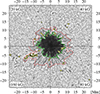 |
Fig. 1. Quadrants of bolometric intensity maps for four selected simulation runs with different initial magnetic field strengths. From top-left clock-wise: B0 = 20 kG, 40 kG, 80 kG, and 160 kG. The magnetic flux is the same for all four runs: F = 1022 Mx. |
As a global property, the size of the penumbrae increased with increasing initial magnetic field strengths, B0, up to 160 kG. Simulation runs with B0 = 20 kG and 40 kG show elongated convective cells resembling penumbral filaments. The B0 = 160 kG run shows the slenderest and longest penumbral filaments, and B0 = 80 kG shows an intermediate state.
Figure 2 and the bottom-right panel of Fig. 4 show the azimuthal averages of the intensity for selected simulations. The vertical dashed lines show the average spot and umbral radii, r, calculated from the contour areas using  . For all simulations, the umbral and spot sizes, along with their penumbral fractions are given in Table 2 (columns ru, rs, and rpu/rs = 1 − ru/rs). Increasing FGauss beyond 1022 Mx increases the sizes of the umbrae and spots. Based on sunspot statistics, Kiess et al. (2014) showed that the umbral radii increase linearly with the spot flux. In our simulations, the umbral radii increased with spot flux, consistent with their linear fit. However, for B0 < 160 kG, the penumbral fractions are smaller than for those with B0 = 160 kG, which, at 47%–52%, are already below the typical value observed in sunspots, where the penumbra covers about 60% of the spot size (e.g. Keppens & Martinez Pillet 1996; Westendorp Plaza et al. 2001; Mathew et al. 2003; Borrero et al. 2004; Bellot Rubio et al. 2004; Sánchez Cuberes et al. 2005; Beck 2008; Borrero & Ichimoto 2011; Chowdhury et al. 2024, and references therein). In summary, our simulations provide sunspots with a realistic umbral size but diminished penumbral length; that is, our simulations provide smaller sunspots than the observed stable ones. However, the simulated spot sizes resemble those of developing sunspots during penumbra formation (see e.g. Jurčák et al. 2014).
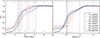 |
Fig. 2. Azimuthally averaged intensity, I/Iqs, (solid lines) as a function of radius in Mm and fraction of the spot radius. The colours indicate the simulations listed in the inset legend. For the older runs (with names ending in ‘o’ in red), the bolometric intensity is shown, and for the other runs (blue), the continuum intensity is shown. Vertical dashed lines show the position of the umbral (left panel with R < 10 Mm, right panel R < 1) and spot boundaries (left panel R > 10 Mm, right panel R = 1 black). The horizontal dashed lines in the right panel show the average umbral intensity. Values corresponding to the location of the vertical dashed lines are given in Table 2, columns ru, rs, ru/s. |
Simulation results.
The difference in brightness in the umbrae between older runs (names ending in ‘o’, red lines in Figs. 2) and the newer ones (blue lines) are caused by the former giving bolometric intensities, I = Ibol; whereas the latter are giving the continuum intensity at 500 nm, I = Ic500. The differences between these intensities are consistent with the expectations of blackbody radiation.
3.2. Surface magnetic fields
In Fig. 3, we plot the radial dependence of the azimuthally averaged Bz for the runs given in the figure’s legend. Simulations with FGauss > 1022 Mx (names ending in ‘c’) have stronger vertical magnetic fields in the spot axis Bz(r = 0) at the average τ = 1 height in the initial condition (see top-left panel of Fig. A.1, three light blue lines) than those with FGauss = 1022 Mx (dark blue line). This results in unrealistically strong fields in the later stages of the simulation (see Fig. 3, blue lines, and the ‘maxBz’ column in Table 2). By unrealistic, we mean that they are stronger than observed on the sun in spots of comparable fluxes (Rezaei et al. 2012; Kiess et al. 2014).
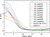 |
Fig. 3. Vertical magnetic field component, Bz, of selected simulations. The Bz value from an observation (green) is also displayed for comparison. |
The initial phase of the simulations had both concentrating and dispersing effects in the magnetic fields at the spot centre. For the B0 = 160 kG simulations starting with the lower resolution (96 / 32 km), the concentrating effects are slightly stronger than the dispersing effects, resulting in a moderate increase in Bz. For the simulation starting with a higher resolution (‘160_opp000h’), the concentrating effects were stronger, resulting in an excessively high Bz. For B0 = 40 kG and 80 kG, the dispersing effects are weaker than those for the B0 = 160 kG simulations, resulting in an overly strong maxBz. This is consistent with a simulation with B0 = 160 kG, but with a closed bottom boundary at the spot foot-point (‘160_opp000b’), which also lacks the very dynamic initial phase with its dispersion effects and has a higher maxBz. The simulation with a closed bottom boundary also lacked a properly formed penumbra and the few elongated granules had inflows along the full length and downflows outside the umbral boundary.
Low-resolution simulations with FGauss = 1022 Mx and B0 = 160 kG have maxBz = 4240 − 4478 G, while Bz drops with increasing radius to values of 200 G similar for all such simulations. Outside the spot, the values for Bz fluctuate, whereas simulations in larger boxes or higher Bopp fluctuate around lower values, as shown in the top left panel of Fig. 4.
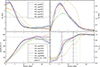 |
Fig. 4. Azimuthal averages of the vertical magnetic field component, Bz (top left), the radial magnetic field component, Br (top right), the inclination (bottom left), and the intensity, Iout (bottom right), of our more realistic simulations (blue, red, black and grey), and of an observation (green), and an old reference simulation (gold). Horizontal dashed lines refer to Bz = 1867 G, the observed critical value for penumbral-type convection to operate (top left), and to an inclination of 90°, meaning a horizontal field (bottom-left). |
Simulations with FGauss > 1022 Mx have increased Br compared to those with FGauss = 1022 Mx. Beyond that, within the spot, all simulations with B0 = 160 kG have a similar dependence of Br on the fractional spot radius, as depicted in the upper right panel of Fig. 4. The B0 = 20 kG simulation has the maximum Br at a larger radius, consistent with the higher umbral fraction. All B0 < 160 kG simulations have a faster drop of Br outside the spot than the B0 = 160 kG simulations. Of the B0 = 160 kG simulations, Br decreases more slowly outside the spot for those in larger boxes, indicating that the drop-off of Br in smaller boxes may be caused by the horizontal periodic boundary conditions.
The increase in field inclination, γ, with fractional spot radius is similar for all B0 = 160 kG simulations up to γ ≈ 80° (Fig. 4, bottom left panel), whereas γ rises more slowly with the fractional spot radius for the B0 < 160 kG simulations, which is consistent with their larger umbral fraction. The other differences in the initial conditions are shown in the bottom right panel of Fig. A.1 within the spot were removed during the dynamic initial phase. Outside the spot, the average inclination fluctuated around 75° −105°, depending on the average Bz there.
3.3. Surface flows
The simulations with B0 = 20 kG and 40 kG have inflows directed towards the umbra along the full length of all elongated convective cells, with downflows at umbral boundaries. Since this is clearly inconsistent with what is observed on the sun, we did not emark on a more detailed discussion of the surface flows in these runs. A comparison of the other runs with observations is given in Sect. 4.
Simulations with B0 = 80 kG and 160 kG and low resolution (96/32 km) have strong in- and downflows in most umbral ends of penumbral filaments (filament heads), with out- and upflows in the middle and outer parts of the filaments. Downflows were also observed between the filaments and at the outer ends. An example map of the radial flows (in- and outflows) and vertical flows (up and down) is presented in Fig. 5.
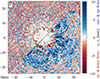 |
Fig. 5. Surface velocity map of sunspot run ‘160_opp000’. Top-left: Vertical flows, vz, downflows in red, upflows in blue. Bottom-right: Radial velocities, vr, inflows in red (towards the spot centre), outflows in blue. The black contours are the same as shown in Fig. 1. |
In the umbra, the dominant contribution to the vertical flows, vz, is an overall oscillation, which at the time shown here is near a zero-crossing and, hence, it is not visible in the map. Our azimuthally averaged and temporally fitted values of vz have these oscillations averaged out over time. This was verified in some simulations by subtracting the τ = 1 surface oscillations from the vertical velocities. Outside the umbra, the averages of the upflow filling factor and separate averages over up- and downflow speeds change quantitatively, but the radial distance of the minima and maxima is not affected. Inside the umbra, these values are not usable because vertical oscillations are the dominant contributors to the velocity.
The following discussion focuses on the common flow behaviour of the B0 = 160 kG simulations. We find that the simulation run with B0 = 80 kG is similar in many aspects, but the shorter penumbral filaments result in slower outflows.
In terms of azimuthal averages, the outflow speed vr, + increases with increasing radius until the spot boundary and then slowly decreases. Inflow speeds of −vr, − increased until the umbral boundary, then converged to the lower quiet sun value. The outflow filling factor, nvr > 0, has values of 39–48% at a local minimum near the umbral boundary, then rapidly increases and tapers off to a maximum around the spot boundary of 88–93% for the B0 = 160 kG simulations. This results in the radial velocity, vr, having a minimum near the umbral boundary and a maximum near the spot boundary. The minima, maxima, and their locations in our simulation runs are listed in Table 2, with vr and vz shown in Fig. 7, where the extrema are marked with + symbols.
Upflow speeds, vz, +, increased steadily with radius until they reached the quiet-sun average at around 1.2 rs. Downflow speeds, −vz, −, have a local speed maximum near the umbral boundary, followed by a decrease in speed over the inner penumbra to increase to the quiet Sun average. Outside the umbral boundary, the upflow filling factor, nvz > 0, increased over the same range as the downflows slowed with increasing radius. Outside this narrow range, any trend in the radial dependence of the filling factor is sufficiently weak to be hidden by any fluctuations that might appear random. The lower panel of (‘160_opp000h’) shows that inside the central umbra, vertical velocities, vz, are, on average, near zero, then drop to a local minimum near the umbral boundary. This is followed by a quick increase over the inner part of the penumbra and a decrease to the quiet sun average over the width of the rest of the penumbra, accompanied by an increase in fluctuations.
Having a negative average quiet-sun vertical velocity does not stand in contradiction to the convective blue shift, since the convective blue shift results from weighting the average of the light, meaning that the bright granular upflows outshine the darker inter-granular downflows. Our average is negative because the τ = 1 surface in the inter-granular lanes is lower; hence, the downflows are faster than the upflows.
The maximal total velocity, v, was found to be outside, but near the spot boundary, beyond which it dropped to the quiet-sun average. Most simulation runs have a minor local maximum near the umbral boundary.
In summary, as shown in Fig. 5, a pattern that appears characteristic of the potential field simulations with B0 ≥ 80 kG presented here is manifested by the bi-directional flows exhibited by the penumbral structure: radial outflows (blue) resembling the observed Evershed flows are present in the mid and outer penumbra, yet the inner penumbra is characterised by strong inflows (red) combined with downflows. Bi-directional flows were first reported in high-resolution observations by Schlichenmaier et al. (2011) as counter-Evershed flows. Recently, García-Rivas et al. (2024) showed that some of these counter-Evershed flows correspond to bi-directional flows that act as a precursor to the formation of a stable penumbra. The simulation with a closed bottom boundary inside the magnetic trunk (‘160_opp000b’) has elongated granules instead of penumbral filaments and, hence, no outflows.
Figure 6 shows that the high-resolution (32/16 km) simulations have, however, both filaments with bi-directional flows and those with normal Evershed flows, meaning upflows in the filament heads, outflows along the whole lengths of the filaments, and downflows at the outer ends and between the filaments. The simulation that started with high-resolution (‘160_opp000h’) has faster outflows (Fig. 7, upper panel), consistent with the resolution dependence of the Evershed flow speed reported by Rempel (2012). The simulation that started at low resolution and was later regridded to high resolution (‘160_opp000ho’) has slower outflows, because the flow speeds decrease over time and this simulation is evaluated at a later time.
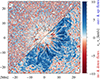 |
Fig. 6. Same as Fig. 5, but for sunspot run ‘160_opp000h’ (high res.), with no spot boundary contour. |
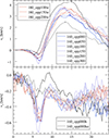 |
Fig. 7. Azimuthally averaged radial, vr (top panel), and vertical, vz (bottom panel) velocities of our more realistic simulations. |
3.4. Flux emergence
Our low-resolution (96/32 km) simulations with B0 = 160 kG and open bottom boundary (names starting with ‘160’ and an ending that does not contain ‘h’ or ‘b’) keep increasing their flux during our observation time (Table 2, column dtF/F, 8.5–13.0%/h). This corresponds to flux emergence. In the only simulation run for substantially longer than 4 h (‘160_opp000’), the stalling of flux emergence at 8–10 h coincides with a narrowing of the penumbra and the disappearance of most outflows.
In simulation ‘160_opp000ho’, for which the data were evaluated 3.5h later than in most other simulations, the flux emergence appears to be tailing off. In the simulation with a closed bottom boundary inside the magnetic trunk (‘160_opp000b’), only slight flux emergence is observed.
4. Summary and conclusion
As the aim of this study is to explore more realistic sunspot simulations by extending the ideas introduced by Nordlund (2015) and examined in Jurčák et al. (2020), we carried out a parameter study in MURaM sunspot simulations under the potential-field initial condition. Here, we varied the following parameters:
-
Initial magnetic field strength, B0: 20, 40, 80, and 160 kG;
-
Magnetic flux content FGauss and opposing flux, Bopp;
-
Box width;
-
Resolution (96 / 32 km versus 32 / 16 km).
Our main results are:
-
The penumbral extent increases systematically with B0, from no penumbra at 20 kG to long, slender filaments at 160 kG.
-
Runs with FGauss > 1022 Mx develop unrealistically large umbral vertical fields, Bz.
-
The most realistic sunspots come from B0 = 160 kG, FGauss = 1022 Mx, which produce (1) maximum Bz = 4.2 − 4.5 kG (still larger than found in observations) and (2) a realistic profile of Bz and Br with the radius.
-
Closing the bottom boundary inside the spot trunk does not create a realistic sunspot.
-
Varying Bopp or the box width changes the background Bz outside the spot but does not significantly affect the internal spot structure or dynamics.
-
For B0 ≤ 40 kG, no Evershed flows develop; there are only in- and downflows, with only slight flux emergence.
-
For B0 = 80 − 160 kG and low resolution (96/32 km), bi-directional flows, resembling those found in observations of the early stages of penumbra formation, are found during ongoing flux emergence.
-
High-resolution (32/16 km) runs produce both filaments with bi-directional flows and filaments with Evershed flows.
From this parameter study, we conclude that simulations initialised with potential-field conditions, sunspot fluxes on the order of 1022 Mx, and strong (160 kG) magnetic fields and open bottom boundary reproduce key aspects of the observed morphology and dynamics of sunspots during the early phases of penumbra formation (see e.g. Schlichenmaier et al. 2010a; Jurčák et al. 2014). Specifically, our simulations have early penumbral-like regions characterised by slender granulation of reduced intensity; rather than exhibiting the classical radial velocities of the Evershed flow (Schlichenmaier & Schmidt 2000; Löhner-Böttcher & Schlichenmaier 2013), they show bi-directional motions that are likely driven by flux emergence at the outskirts of the spot (García-Rivas et al. 2024). These results highlight the value of these simulations in investigating the initial stages of sunspot formation.
Comparisons with failed simulations show that – at least for low-resolution simulations with potential field top boundary conditions – we only get a realistic-looking sunspot with outwards flow in a sufficiently wide penumbra, while flux keeps emerging in the outer parts of the spot.3 We speculate that any low-density plasma in ∩-shaped magnetic field lines below the surface might be sufficient to drive flux emergence and create penumbrae as in our simulations.
However, observations suggest that an overlying canopy is required to form a stable penumbra with Evershed flows (Lindner et al. 2023; Chifu et al. 2025). Older simulations have achieved this by forcing the field to be more inclined at the top boundary, so that the inclined field drives the Evershed flows. The presence of Evershed flows in some of the filaments of our high-resolution simulations, coupled with their absence in low-resolution simulations, indicates that insufficient resolution is an inhibiting factor for Evershed flows, in line with preliminary reports from Rempel & Hotta (2025). We speculate that embedding the spot in a much larger simulation box (across all dimensions above and below the photosphere), while including a small-scale dynamo run that allows a canopy to form naturally, might also force the field to be sufficiently inclined. As a result, Evershed flows might indeed form even in low-resolution simulations if the spot is placed in the right location.
Acknowledgments
We thank the anonymous reviewer for their valuable and insightful comments, which helped improve this manuscript. This work was supported by the Czech-German common grant, funded by the Czech Science Foundation under project 23-07633K and by the Deutsche Forschungsgemeinschaft under project BE 5771/3-1 (eBer-23-13412), and the institutional support ASU:67985815 of the Czech Academy of Sciences. Most of the simulations leading to the results obtained were run on Piz Daint at the Swiss National Supercomputing Centre, Switzerland, financed through the ACCESS programme of the SOLARNET project, which has received funding from the European Union Horizon 2020 research and innovation programme under grant agreement no 824135. For the older simulations, we would like to thank Matthias Rempel for providing us with their data and acknowledge the high-performance computing support from Cheyenne (doi:10.5065/D6RX99HX) provided by the NFS NCAR’s Computational and Information Systems Laboratory, sponsored by the National Science Foundation. This research has made use of NASA’s Astrophysics Data System Bibliographic Services.
References
- Beck, C. 2008, A&A, 480, 825 [NASA ADS] [CrossRef] [EDP Sciences] [Google Scholar]
- Bellot Rubio, L. R., Balthasar, H., & Collados, M. 2004, A&A, 427, 319 [NASA ADS] [CrossRef] [EDP Sciences] [Google Scholar]
- Bhatia, T. S., Panja, M., Cameron, R. H., & Solanki, S. K. 2025, A&A, 693, A264 [NASA ADS] [CrossRef] [EDP Sciences] [Google Scholar]
- Borrero, J. M., & Ichimoto, K. 2011, Liv. Rev. Sol. Phys., 8, 4 [Google Scholar]
- Borrero, J. M., Solanki, S. K., Bellot Rubio, L. R., Lagg, A., & Mathew, S. K. 2004, A&A, 422, 1093 [NASA ADS] [CrossRef] [EDP Sciences] [Google Scholar]
- Chen, F., Rempel, M., & Fan, Y. 2017, ApJ, 846, 149 [Google Scholar]
- Cheung, C. M. M. 2006, Ph.D. Thesis, Georg August University of Göttingen, Germany http://dx.doi.org/10.53846/goediss-2790 [Google Scholar]
- Cheung, M. C. M., Rempel, M., Title, A. M., & Schüssler, M. 2010, ApJ, 720, 233 [Google Scholar]
- Chifu, I., Bello González, N., & Jurčák, J. 2025, A&A, 699, A218 [NASA ADS] [CrossRef] [EDP Sciences] [Google Scholar]
- Chowdhury, P., Kilcik, A., Saha, A., et al. 2024, Sol. Phys., 299, 19 [Google Scholar]
- García-Rivas, M., Jurčák, J., Bello González, N., et al. 2024, A&A, 686, A112 [NASA ADS] [CrossRef] [EDP Sciences] [Google Scholar]
- Heinemann, T., Nordlund, Å., Scharmer, G. B., & Spruit, H. C. 2007, ApJ, 669, 1390 [Google Scholar]
- Hotta, H., & Iijima, H. 2020, MNRAS, 494, 2523 [Google Scholar]
- Jurčák, J., Bellot Rubio, L. R., & Sobotka, M. 2014, A&A, 564, A91 [Google Scholar]
- Jurčák, J., Schmassmann, M., Rempel, M., Bello González, N., & Schlichenmaier, R. 2020, A&A, 638, A28 [NASA ADS] [CrossRef] [EDP Sciences] [Google Scholar]
- Keppens, R., & Martinez Pillet, V. 1996, A&A, 316, 229 [NASA ADS] [Google Scholar]
- Kiess, C., Rezaei, R., & Schmidt, W. 2014, A&A, 565, A52 [NASA ADS] [CrossRef] [EDP Sciences] [Google Scholar]
- Lindner, P., Kuckein, C., González Manrique, S. J., et al. 2023, A&A, 673, A64 [NASA ADS] [CrossRef] [EDP Sciences] [Google Scholar]
- Löhner-Böttcher, J., & Schlichenmaier, R. 2013, A&A, 551, A105 [NASA ADS] [CrossRef] [EDP Sciences] [Google Scholar]
- Ludwig, H.-G. 1992, Ph.D. Thesis, Christian-Albrechts-Universität zu Kiel [Google Scholar]
- Mathew, S. K., Lagg, A., Solanki, S. K., et al. 2003, A&A, 410, 695 [NASA ADS] [CrossRef] [EDP Sciences] [Google Scholar]
- Nordlund, A. 1982, A&A, 107, 1 [Google Scholar]
- Nordlund, Å. 2015, Nordita Seminar on Sunspot Formation: Theory, Simulations and Observations [Google Scholar]
- Panja, M., Cameron, R., & Solanki, S. K. 2020, ApJ, 893, 113 [CrossRef] [Google Scholar]
- Panja, M., Cameron, R. H., & Solanki, S. K. 2021, ApJ, 907, 102 [Google Scholar]
- Rempel, M. 2012, ApJ, 750, 62 [Google Scholar]
- Rempel, M. 2014, ApJ, 789, 132 [Google Scholar]
- Rempel, M. 2017, ApJ, 834, 10 [Google Scholar]
- Rempel, M., & Hotta, H. 2025, in SDO 2025 Science Workshop, Boulder, Colorado, presentation nr. 13 [Google Scholar]
- Rempel, M., Schüssler, M., Cameron, R. H., & Knölker, M. 2009a, Science, 325, 171 [CrossRef] [Google Scholar]
- Rempel, M., Schüssler, M., & Knölker, M. 2009b, ApJ, 691, 640 [Google Scholar]
- Rezaei, R., Beck, C., & Schmidt, W. 2012, A&A, 541, A60 [NASA ADS] [CrossRef] [EDP Sciences] [Google Scholar]
- Sánchez Cuberes, M., Puschmann, K. G., & Wiehr, E. 2005, A&A, 440, 345 [NASA ADS] [CrossRef] [EDP Sciences] [Google Scholar]
- Scharmer, G. B., Nordlund, Å., & Heinemann, T. 2008, ApJ, 677, L149 [NASA ADS] [CrossRef] [Google Scholar]
- Scherrer, P. H., Schou, J., Bush, R. I., et al. 2012, Sol. Phys., 275, 207 [Google Scholar]
- Schlichenmaier, R., & Schmidt, W. 2000, A&A, 358, 1122 [NASA ADS] [Google Scholar]
- Schlichenmaier, R., Bello González, N., Rezaei, R., & Waldmann, T. A. 2010a, Astron. Nachr., 331, 563 [NASA ADS] [CrossRef] [Google Scholar]
- Schlichenmaier, R., Rezaei, R., Bello González, N., & Waldmann, T. A. 2010b, A&A, 512, L1 [NASA ADS] [CrossRef] [EDP Sciences] [Google Scholar]
- Schlichenmaier, R., González, N. B., & Rezaei, R. 2011, in Physics of Sun and Star Spots, eds. D. Prasad Choudhary, & K. G. Strassmeier, IAU Symposium, 134 [Google Scholar]
- Schmassmann, M., Schlichenmaier, R., & Bello González, N. 2018, A&A, 620, A104 [NASA ADS] [CrossRef] [EDP Sciences] [Google Scholar]
- Schmassmann, M., Rempel, M., Bello González, N., Schlichenmaier, R., & Jurčák, J. 2021, A&A, 656, A92 [NASA ADS] [CrossRef] [EDP Sciences] [Google Scholar]
- Schmassmann, M., Bello González, N., Jurčák, J., & Schlichenmaier, R. 2026, A&A, 706, A218 [NASA ADS] [CrossRef] [EDP Sciences] [Google Scholar]
- Spruit, H. C. 1981, in The Physics of Sunspots, eds. L. E. Cram, & J. H. Thomas, 98 [Google Scholar]
- Tiwari, S. K., van Noort, M., Lagg, A., & Solanki, S. K. 2013, A&A, 557, A25 [NASA ADS] [CrossRef] [EDP Sciences] [Google Scholar]
- Vögler, A., Bruls, J. H. M. J., & Schüssler, M. 2004, A&A, 421, 741 [NASA ADS] [CrossRef] [EDP Sciences] [Google Scholar]
- Westendorp Plaza, C., del Toro Iniesta, J. C., Ruiz Cobo, B., et al. 2001, ApJ, 547, 1130 [Google Scholar]
These unphysically strong initial fields at the bottom of the box get quickly reduced by an initial transient.
Radial in sunspot simulations refers to a cylindrical coordinate system, with z aligned with the spot axis and increasing with height.
The causes behind the flux emergence in our simulations relate to the unphysical entropy enhancement during the initial transient and are beyond the scope of this article.
Appendix A: Initial magnetic field configurations
Figure A.1 shows the azimuthal averages of the initial magnetic field at the average height of the τ = 1 iso-surface in the quiet Sun. The top two panels (Bz + Bopp and Br), show the initial conditions for all our simulations (except ‘80_opp000o’ and ‘alpha*’), because introducing a Bopp ≠ 0 only offsets Bz uniformly, and does not affect Br. In the bottom right panel, all simulations (except ‘alpha*’) are plotted. Colours and line-styles are described in Table A.1, where the ‘?’ in ‘160_opp000?’ is a wildcard, standing for any of ‘o’, ‘ho’, ‘h’, ‘’, or ‘b’, since these simulations share the same initial conditions.
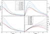 |
Fig. A.1. Initial magnetic field. Vertical field Bz + Bopp (top left), radial field Br (top right), total field |B| (bottom left), and inclination to the surface normal γ. The legend in the top left panel shows the simulations plotted in the first three panels. The legend in the bottom right panel gives a selection of the simulations shown there, the rest is given in Table A.1; for each line in that table (colour), the further right the column is (the higher B0 or Bopp, the changing numbers in the run names), the higher the inclination. |
Colours and line styles for simulations given in bottom right panel of Fig. A.1, showing the inclination in the initial field.
While this figure shows many details, primarily the following aspects are pertinent:
-
1)
FGauss > 1022 Mx leads to strong Bz on the spot axis.
-
2)
w = 98.304 Mm leads to the field being distributed over a wider box, resulting in a weaker Bz far from the spot axis and more extended Br.
-
3)
The inclinations in the initial conditions show a wide range of behaviour, in particular outside the spot.
All Tables
Colours and line styles for simulations given in bottom right panel of Fig. A.1, showing the inclination in the initial field.
All Figures
|
Fig. 1. Quadrants of bolometric intensity maps for four selected simulation runs with different initial magnetic field strengths. From top-left clock-wise: B0 = 20 kG, 40 kG, 80 kG, and 160 kG. The magnetic flux is the same for all four runs: F = 1022 Mx. |
| In the text | |
|
Fig. 2. Azimuthally averaged intensity, I/Iqs, (solid lines) as a function of radius in Mm and fraction of the spot radius. The colours indicate the simulations listed in the inset legend. For the older runs (with names ending in ‘o’ in red), the bolometric intensity is shown, and for the other runs (blue), the continuum intensity is shown. Vertical dashed lines show the position of the umbral (left panel with R < 10 Mm, right panel R < 1) and spot boundaries (left panel R > 10 Mm, right panel R = 1 black). The horizontal dashed lines in the right panel show the average umbral intensity. Values corresponding to the location of the vertical dashed lines are given in Table 2, columns ru, rs, ru/s. |
| In the text | |
|
Fig. 3. Vertical magnetic field component, Bz, of selected simulations. The Bz value from an observation (green) is also displayed for comparison. |
| In the text | |
|
Fig. 4. Azimuthal averages of the vertical magnetic field component, Bz (top left), the radial magnetic field component, Br (top right), the inclination (bottom left), and the intensity, Iout (bottom right), of our more realistic simulations (blue, red, black and grey), and of an observation (green), and an old reference simulation (gold). Horizontal dashed lines refer to Bz = 1867 G, the observed critical value for penumbral-type convection to operate (top left), and to an inclination of 90°, meaning a horizontal field (bottom-left). |
| In the text | |
|
Fig. 5. Surface velocity map of sunspot run ‘160_opp000’. Top-left: Vertical flows, vz, downflows in red, upflows in blue. Bottom-right: Radial velocities, vr, inflows in red (towards the spot centre), outflows in blue. The black contours are the same as shown in Fig. 1. |
| In the text | |
|
Fig. 6. Same as Fig. 5, but for sunspot run ‘160_opp000h’ (high res.), with no spot boundary contour. |
| In the text | |
|
Fig. 7. Azimuthally averaged radial, vr (top panel), and vertical, vz (bottom panel) velocities of our more realistic simulations. |
| In the text | |
|
Fig. A.1. Initial magnetic field. Vertical field Bz + Bopp (top left), radial field Br (top right), total field |B| (bottom left), and inclination to the surface normal γ. The legend in the top left panel shows the simulations plotted in the first three panels. The legend in the bottom right panel gives a selection of the simulations shown there, the rest is given in Table A.1; for each line in that table (colour), the further right the column is (the higher B0 or Bopp, the changing numbers in the run names), the higher the inclination. |
| In the text | |
Current usage metrics show cumulative count of Article Views (full-text article views including HTML views, PDF and ePub downloads, according to the available data) and Abstracts Views on Vision4Press platform.
Data correspond to usage on the plateform after 2015. The current usage metrics is available 48-96 hours after online publication and is updated daily on week days.
Initial download of the metrics may take a while.