| Issue |
A&A
Volume 708, April 2026
|
|
|---|---|---|
| Article Number | A207 | |
| Number of page(s) | 14 | |
| Section | Stellar atmospheres | |
| DOI | https://doi.org/10.1051/0004-6361/202658929 | |
| Published online | 06 April 2026 | |
A fast method for deriving relative small-scale magnetic field variations from high-resolution spectroscopy
1
Leiden Observatory, Leiden University,
PO Box 9513,
2300 RA
Leiden,
The Netherlands
2
Center for Astrophysics | Havard & Smithsonian,
60 Garden Street,
Cambridge,
MA
02138,
USA
★ Corresponding author: This email address is being protected from spambots. You need JavaScript enabled to view it.
Received:
12
January
2026
Accepted:
27
February
2026
Abstract
Context. Setting observational constraints on stellar magnetic fields is essential for both stellar and planetary physics. They play a key role in the formation and evolution of stars and planets, and they are responsible for spurious signals in radial velocity curves that impact the detection and characterization of exoplanets. Recent observations have revealed the diversity and evolution of large-scale magnetic fields in low-mass stars. However, these large-scale fields only account for a small fraction of the observed unsigned magnetic flux. The other crucial stellar magnetism information originates from (spatially) small-scale magnetic fields, which account for most of the surface magnetic flux and exhibit a clear temporal evolution on timescales of many years.
Aims. With this work, we aim to develop new fast techniques to extract small-scale magnetic field estimates from time series of observed high-resolution spectra. One objective is to develop tools that will enable the community to take full advantage of the upcoming monitoring surveys carried out with various high-resolution spectrometers. Our ultimate goal is to study the temporal evolution of small-scale magnetic fields and offer insights into the magnetic properties of low-mass stars and their magnetic cycles.
Methods. We implemented a process to capture relative pixel variations caused by changes in magnetic field strengths, relying on synthetic spectra computed with ZeeTurbo. This approach provides extremely fast and reliable estimates of relative magnetic field strength variations from series of high-resolution spectra, mitigating the impact of systematics between models and observations. We assessed the performance of the proposed method through its application to simulated data and publicly available observed spectra recorded with SPIRou, Narval, and ESPaDOnS. In addition, we implemented a model-driven process to derive relative temperature variations and we explored the influence magnetic fields have on these measurements.
Results. Our results are in excellent agreement with the magnetic field estimates previously obtained from spectra recorded with SPIRou. This method provides robust constraints on the structure of the magnetic field variations and proves to be relatively insensitive to small changes in the assumed atmospheric parameters and broadening. We find that magnetic field variations have the potential of introducing biases in relative temperature estimates. This is particularly relevant in the case of the Narval/ESPaDOnS spectral domains, which contain a large number of magnetically sensitive transitions and where contrast is more important. Our application to archival data provides new constraints on the evolution of small-scale magnetic fields and underscores the potential of the proposed method for analyzing data in the context of large observation programs.
Conclusions. By reducing the problem to a set of linear equations, our method offers extremely fast results, making it viable for integration in future pipelines developed for large spectroscopic surveys. These estimates will provide much needed information to correct radial velocity curves and constrain dynamo processes.
Key words: techniques: spectroscopic / stars: low-mass / stars: magnetic field
© The Authors 2026
 Open Access article, published by EDP Sciences, under the terms of the Creative Commons Attribution License (https://creativecommons.org/licenses/by/4.0), which permits unrestricted use, distribution, and reproduction in any medium, provided the original work is properly cited.
This article is published in open access under the Subscribe to Open model. This email address is being protected from spambots. You need JavaScript enabled to view it. to support open access publication.
1 Introduction
Sun-like stars and M dwarfs are known to host magnetic fields (e.g., Saar & Linsky 1985; Johns-Krull & Valenti 1996; Kochukhov 2021 ; Reiners et al. 2022) that have consequences on their polarized and unpolarized spectra. These fields are thought to be responsible for activity phenomena, introducing spurious signal in radial velocity (RV) measurements (Dumusque et al. 2021; Bellotti et al. 2022) and consequently impacting exoplanet detection and characterization. Magnetic fields also play a crucial role in stellar formation and evolution processes (Donati & Landstreet 2009), leading to angular momentum loss (e.g., Skumanich 1972; Vidotto et al. 2014) and surface inhomogeneities (e.g., spots, plages, and faculae).
M dwarfs are the most numerous stars in the solar neighborhood (Reylé et al. 2021) and they are considered prime targets for the search of habitable exoplanets. The precise and accurate characterization of these stars is essential to extract reliable estimates on the masses and radii of the exoplanets orbiting them (Bonfils et al. 2013; Dressing & Charbonneau 2015; Gaidos et al. 2016). The masses of M dwarfs range from 0.08 to 0.57 M⊙ (Pecaut & Mamajek 2013): stars with masses below 0.35 M⊙ are believed to be fully convective (Chabrier & Baraffe 1997), while M dwarfs with masses above 0.35 M⊙ have radiative interiors and an outer convective envelope separated by a transition region known as the tachocline (Spiegel & Zahn 1992). The tachocline is thought to play a key role in the 22-year magnetic cycle observed in the Sun (see Parker 1955; Charbonneau 2010). In fully convective M dwarfs, dynamo processes must be revisited and alternative scenarios have been proposed to generate large-scale fields without the need for a tachocline (Chabrier & Küker 2006; Yadav et al. 2015).
The last decade has been marked by the rapid development of high-resolution spectrometers, including several near-infrared instruments such as CARMENES (Quirrenbach et al. 2014), CRIRES+ (Dorn et al. 2023), and SPIRou (Donati et al. 2020), motivated in part by the search for exoplanets around M dwarfs. The spectropolarimetric capabilities of some of these instruments have led to numerous studies focused on large-scale stellar magnetic fields (e.g., Kochukhov & Reiners 2020; Finociety et al. 2023; Donati et al. 2023b; Bellotti et al. 2024), while unpolarized spectra have enabled the community to characterize the small-scale magnetic fields of low-mass stars (e.g., Shulyak et al. 2017; Reiners et al. 2022; Cristofari et al. 2023a,b). Combined efforts to characterize both large-scale and small-scale magnetic fields have provided a complete picture of cool stars magnetism (e.g., Kochukhov & Lavail 2017; Donati et al. 2023a, 2025; Bellotti et al. 2025). Recent works have reported efforts to characterize the variation of small-scale magnetic fields throughout observation campaigns lasting several years (Donati et al. 2023a; ?) and revealing rotational modulation and long-term fluctuations. Small-scale magnetic fields have been proposed as an excellent proxy to correct for activity jitters in radial velocity curves (Haywood et al. 2016, 2022). The extraction of small-scale field fluctuations from the high-resolution spectra, particularly from the spectra used to obtain radial velocity curves, is therefore timely.
With this work, we propose a new process for deriving variations in the average surface magnetic field strength (〈B〉) throughout time series of spectra. We validate our method and assess its performance on simulated spectra before applying it to archival observed spectra. Section 2 describes the observational data used in this study. Our method and its implementation are described in Sects. 3 and 4. The application of our method to observed spectra is described in Sect. 5 and our results are discussed in Sect. 6.
2 Observations and data reduction
This work takes advantage of public high-resolution spectroscopic observations obtained with three instruments: ESPaDOnS (Donati et al. 2006) and SPIRou (Donati et al. 2020), installed at the Canada-France Hawaii-Telescope (CFHT), and Narval installed on the Télescope Bernard Lyot (TBL) at the Pic du Midi observatory, France (Donati 2003).
ESPaDOnS and Narval data were reduced with the LIBRE-ESPRIT reduction software (Donati et al. 1997) and the continuum-normalized spectra were retrieved from Polarbase (Petit et al. 2014). SPIRou data were reduced with APERO (Cook et al. 2022) and downloaded from the Canadian Astrophysics Data Center (CADC). APERO provides multiple data products including spectra before and after correction of telluric lines (with extention e.fits and t.fits, respectively), along with blaze profiles estimated from flat-field exposures. An estimate of the photon noise was obtained from the number counts prior to telluric correction and used to estimate uncertainties in the telluric-corrected spectra.
For this work, we refined our initial spectrum normalization procedure of SPIRou spectra, used by Cristofari et al. (2023b, 2025). For each observation, the spectral orders were corrected by the blaze profiles and a 1D spectrum was obtained by merging all orders. In cases where spectral orders overlapped, only the segments with the highest throughput were kept to avoid biases of the normalization by noisy order edges. The blaze-corrected spectrum was then divided in windows of equal velocity width (which we empirically fixed to 3000 km s−1). In each window, we computed the flux 95th percentile and a cubic interpolation between the obtained points provided us with the continuum of the whole spectrum. Our process successfully captured low-frequency variation in the spectra, while preserving the structure of the spectral lines. We find that this process is particularly useful in preserving the shape of spectral lines recorded on an order edge, which can bias normalization in order-per-order normalization schemes.
Here, we consider three M dwarfs: EV Lac, DS Leo, and Barnard’s star. All their available SPIRou spectra were retrieved and combined for each observation night to achieve higher signal-to-noise ratios (S/Ns). Most of the observations recorded with SPIRou were obtained in the context of the SPIRou Legacy Survey. For EV Lac and DS Leo, we additionally retrieved all of the available Narval and ESPaDOnS data. Regions with deep telluric absorption bands were excluded from the analysis. Because both instruments have similar characteristics, observations were used together, and spectra were combined each night to obtain higher S/Ns. For EV Lac, this yielded spectra for 67 nights between 2005 to 2016 and for DS Leo, this yielded spectra for 61 nights between 2006 and 2014.
3 Model description
The idea of extracting information about the stellar surface from relative variations in spectral features has been around for decades, with Gray & Johanson (1991); Gray (1994) selecting highly Teff-sensitive line ratios to derive temperature variations. Some recent studies have been focused on deriving relative radial velocity variations to achieve the meter-per-second precisions needed to detect and characterize exoplanets (see, e.g., Artigau et al. 2022; Shahaf & Zackay 2023). More recently, Artigau et al. (2024) proposed deriving relative temperature variations from a fully data-driven approach and relying on the formalism adopted by Bouchy et al. (2001) and Artigau et al. (2022). We begin by briefly reviewing the basis of this formalism.
We consider a spectrum, A, function of a parameter, x, which is assumed to have a single value for all pixels (e.g., effective temperature, metallicity, magnetic field intensity). Small variations between A and a reference spectrum, Aref, can be approximated by the derivative of A with respect to x evaluated at xref, so that
 (1)
(1)
This approach provides a robust method to derive the variation of any quantity responsible for fluctuations in a spectrum as long as the derivative for each pixel is known and that the variations are small. Artigau et al. (2024) relied on this formalism to search for temperature variations, deriving ∂A/∂T from grids of observed spectra.
In the context of magnetic fields, however, the implementation of this method leads to spurious results, which we attribute to two main factors. First, for most pixels, variations in flux as a function of magnetic field in the 0-10 kG range are poorly modeled by a low-order polynomial; as a result, the assumption of small variations fails. Secondly, observed spectra are poorly modeled by a single magnetic field intensity (see, e.g., Kochukhov 2021; Reiners et al. 2022; Cristofari et al. 2023a,b). To overcome these limitations, it is necessary to adopt a more complete formalism describing the variation of pixels with magnetic field intensity for different magnetic components.
3.1 Formalism
In this section, we describe the now commonly used formalism (see, e.g. Shulyak et al. 2014, 2019; Reiners et al. 2022; Cristofari et al. 2023a,b) that we adopted. Here, spectrum A is represented as
 (2)
(2)
where Fk is the synthetic disk-integrated spectrum of a star with an assumed radial magnetic field strength and αk is the filling factor associated with that component. Previous studies suggest a range of useful components for M dwarfs spanning 0 kG to 12 kG (Shulyak et al. 2019; Reiners et al. 2022; Cristofari et al. 2023a). Because the filling factors must add up to 1 for the problem to remain physical, this relation can be written as
 (3)
(3)
where F0 is the synthetic disk-integrated spectrum computed for a 0 kG magnetic field. The synthetic spectrum A therefore depends solely on the filling factors, ak, associated with each magnetic component. Let us consider a reference spectrum, Aref, described by the filling factors, εk, so that  . Then a variation between A and Aref can be written as
 (4)
(4)
The variation in flux can be described by a variation in filling factors ak - εk, which we denote as δak hereafter. The variation in surface averaged magnetic field strength, 〈B〉, can then simply be obtained as  , where Bk is the magnetic field strength for the k-th component.
Solving Eq. (4) allows us to derive δak, provided that the values of A, Aref, and Fk for each magnetic components are known. In our application to observed spectra, the reference spectrum, Aref, was computed from the observed spectra directly, so the left hand-side of Eq. (4) comes from observations, while the right-hand side of the equation is informed by models (see Sect. 4).
4 Implementation and simulations
Our implementation relies on synthetic spectra computed with ZeeTurbo (Cristofari et al. 2023a), which allowed us to obtain Fk - F0 for different field strengths. Synthetic spectra were computed with higher sampling than observations, so that for an observed spectrum A, we can choose the pixels in Fk - F0 corresponding to the nearest observed wavelengths. We built the reference spectrum Aref by taking the median of the observed spectra in the stellar reference frame, which we refer to as the template hereafter. Our process is inherently sensitive to spurious pixels in the observations and flux fluctuations not properly accounted for by error bars (e.g., telluric line residuals). To mitigate the impact of spurious pixels, we quadratically added the standard deviation of the flux across the series of observed spectra to the photon noise associated with each pixel. We then implemented an iterative process to reject bad pixels. Specifically, the weighted least-squares problem (Eq. (4)) can be solved using all points to obtain a first estimate of the δak, which is used to make a prediction on the variation of each pixel’s flux. We then computed the reduced χ2 on the predicted and observed flux variations and used this value to inflate the error bars associated with each pixel. We rejected each pixel for which the flux ends up deviating by more than three times the inflated error bar and the weighted least-square problem was solved on the remaining pixels. The process was repeated until all spurious pixels are rejected. Convergence was typically reached within the first ten iterations in our applications. This approach provides a robust and conservative way to reject bad pixels that could impact the results. We find that this method is particularly robust to provide estimates for spectra with significant artifacts.
4.1 Application to simulated spectra
We constructed a series of “synthetic observations”, relying on synthetic spectra computed with ZeeTurbo. We relied on the results from Cristofari et al. (2025) to extract realistic fillingfactor distributions for the relevant series of observation nights. Consequently, we built synthetic observations from linear combinations of models computed for magnetic field strengths ranging from 0 to 10 kG in steps of 2 kG. Additionally, we relied on temperature variation estimates (δT) obtained with the LBL package (Artigau et al. 2024) from the same data to simulate the impact of temperature variations at the stellar surface, which have been shown to be significantly anti-correlated with surface averaged magnetic field variations (δ〈B〉) for the stars considered in this work (Cristofari et al. 2025). The modeled spectra were convolved with a Gaussian profile of full width at half maximum (FWHM) of 4.3 kms−1 (to mimic the instrumental width of SPIRou), followed by a second Gaussian profile of 5.0km s−1 to represent the typical broadening associated with rotation and macroturbulence for a star such as EV Lac (see Sect. 5). We note that convolutions can only approximately reproduce the impact of rotation or macro-turbulence on spectra, especially for lines with complex Zeeman patterns. The current method, however, relies on the relative variation of fluxes as a function of field strength, mitigating the impact of the approximation. Relying on convolution enables faster computations and our method proves relatively insensitive to broadening (see Sect. 4.4). We note that detailed disk integration could be added in future implementations. The broadened synthetic spectra were then re-binned on a wavelength grid typical for spectra recorded with SPIRou or Narval. Additional series of models were obtained by considering either magnetic field variations or temperature variations alone. Our process was applied to the synthetic observations, relying on different assumptions to assess the behavior of our method and its sensitivity to various parameters.
4.2 Sensitivity to normalization
Low-frequency fluctuations are often observed in echelle spectra, with the potential to lead to biased δ〈B〉 and δT estimates. While an absolute normalization of the continuum is not necessary, relative normalization with respect to the reference spectrum is crucial to obtain accurate results with the proposed method.
To mitigate the impact of low-frequency continuum fluctuations, a moving median with a width of 500 km s−1 was applied to the residuals between each observed spectrum and the template. The resulting continuum variations were used to correct each individual observation. We tested the impact of such a normalization step by applying it to our series of synthetic observations. Specifically, we applied rolling medians with different window sizes to synthetic observations and applied our method with and without filtering the models used to compute Fk - F0.
Our simulations reveal that if our process is applied to median-filtered observations without filtering the models, the amplitude of the retrieved fluctuations are “damped”, meaning that the structure of the variations is conserved, but their amplitude is reduced (see Fig. 1, red squares). This effect can be mitigated by filtering the models used to compute Fk - F0 with a rolling median of similar window size (see Fig. 1, green + symbols). We note that such filtering is not perfect, in particular when applied to spectral regions containing broad or blended lines. We found that applying a rolling median to the residuals between the models and model of reference (e.g., to Fk - F0 directly) provides the most robust results, as this limits the changes in pseudocontinuum caused by broad absorption features. Furthermore, we note that strong magnetic fields can significantly broaden the absorption features, fundamentally changing the shape of observed pseudo-continuum. Consequently, one may favor larger windows for the rolling median to avoid introducing spurious feature variations in the models.
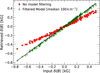 |
Fig. 1 Comparison between the retrieved (y-axis) and input (x-axis) relative magnetic field strengths (δ〈B〉). The synthetic observations were normalized to the template using a rolling median with a window of 100km s−1. The red squares and green plus symbols (‘+’) show the results obtained before and after re-normalizing the models used to computed Fk - F0 (Eq. (4)) with a 100 km s−1 median filter, respectively (see text). The black line marks the equality. This figure illustrates the need for careful re-normalization of the models to avoid biases in the results. |
4.3 Relation between temperature and magnetic fields
Recent results have provided strong evidence of anti-correlations between the obtained small-scale field measurements and temperature variations (δT) for a few strongly magnetic targets (Artigau et al. 2024; Cristofari et al. 2025). In this work, we investigate the impact of temperature variations on magnetic field estimates and vice versa.
To retrieve the temperature variations, we implemented a process similar to that described by Artigau et al. (2024), with the notable difference that we derived ∂A/∂T for each pixel from our synthetic spectra. To validate our process, we created a series of modeled observations with varying effective temperatures, following the estimate obtained with the LBL approach for EV Lac (with typical variations of less than 20 K). Our implementation allows us to successfully retrieve the temperature variations used to generate the models.
To investigate the impact of magnetic fields on temperature variation estimates, we modeled the spectra, accounting for both temperature and magnetic fields variations by taking realistic estimates for EV Lac from Cristofari et al. (2025). The average surface magnetic field strengths then ranged from 4 to 5 kG, and the effective temperatures range from 3290 to 3310 K. We found that temperature variations have a limited impact on the derived δ〈B〉. The inclusion of magnetic fields, however, was shown to have a much more significant impact on the derived δT (see Fig. 2). We found that this impact is particularly significant for simulations covering the Narval/ESPaDOnS wavelength domain, where a very large number of atomic features are predicted to be sensitive to magnetic fields.
The results of this experiment show that δT and δ〈B〉 estimates are not completely independent, with a greater sensitivity of δT estimates to magnetic field variations seen for realistic conditions. We note that typical δT are small, with a few kelvin variations leading to small changes in the observed spectra, while δ〈B〉 fluctuations in stars like EV Lac can lead to more visible pixel variations. Furthermore, magnetic field variations in stellar spectra lead to effects that are strongly dependent on the considered spectral line. Having both magnetically sensitive and insensitive lines in the spectral domain makes it possible to obtain robust constraints on δ{B). A comparison between the model-driven and data-driven δT estimates is discussed in Sect. 5.3.
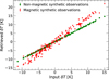 |
Fig. 2 Comparison between the retrieved δT (y-axis) and the input δT used to generate the synthetic observations (x-axis). Synthetic observations were computed on the wavelength range covered by Narval/ESPaDOnS, accounting for magnetic field variations (red squares), or fixing the value of the magnetic fields to 0 kG (green circles). This figure illustrates how magnetic fields can impact the δT estimates. |
4.4 Impact of atmospheric parameters on 〈B〉 variations
We investigated the impact that incorrect assumptions on the atmospheric properties of the star can have on the results. To achieve this, modeled observations were analyzed with Fk - F0 computed for different effective temperatures (Teff), surface gravities (log g), metallicities ([M/H]), and projected rotational velocity (v sin i).
We find that an offset in atmospheric parameters has a ‘damping’ effect on the retrieved relative field strengths, similar to the impact of short-window normalization (see Sect. 4.2): the structure of the variations are typically conserved, while the amplitude of the field variations are either lower or higher than expected. Through simulations, we find that a change of 300 K can yield a maximum difference in δ〈B〉 of 0.1 kG in the case of EV Lac (whose magnetic field is able to change by up to 1 kG in our simulations), comparable to the typical uncertainties reported in Cristofari et al. (2025). Similarly, changes of 0.5 dex in the assumed surface gravity or metallicity can lead to maximum differences in δ〈B〉 of 0.2 kG. Changes in the assumed broadening of the spectra of up to 5 km s−1 typically lead to maximum changes in δ〈B〉 of 0.05 kG. The typical uncertainties on Teff, log g, [M/H] and v sin i are generally lower than 300 K, 0.5 dex or 5 km s−1, while the maximum differences in δ<B) are then lower than the typical uncertainties associated with the measurements. Our process remains therefore robust to changes in atmospheric parameters and broadening, which allows us to limit the impact of incorrect stellar characterization on the results.
Atmospheric parameters adopted in the current work.
5 Application to observations
5.1 Application to SPIRou spectra
We applied our process to spectra recorded with SPIRou for EV Lac, DS Leo, and Barnard’s star, whose small-scale magnetic fields were previously characterized from fits of synthetic spectra to each individual observation (Cristofari et al. 2025). This allowed us to make direct comparisons between the obtained δ<B) and the magnetic field estimates reported by Cristofari et al. (2025). For each star, we assumed atmospheric parameters that were close to those obtained by Cristofari et al. (2025), which we list in Table 1. The broadening parameters (i.e., turbulence, rotation, instrumental width) were approximated by a single Gaussian profile. While the finetuning of each of these parameters is possible, we chose to keep the assumed atmospheric parameters and broadening kernels approximate, given the relative insensitivity of the proposed method to detailed stellar characterization (see Sect. 4.4).
For all three stars, we obtained magnetic field variations that were in very good agreement with the results of Cristofari et al. (2025, as also seen in our Figs. 3 and C.1), with reduced χ2 values between the two series of points of 1.01, 1.07, and 1.26. In addition, we obtained Pearson correlation coefficients of 0.97, 0.89, and 0.58 for EV Lac, DS Leo, and Barnard’s star, respectively. Relying on the same tools as Cristofari et al. (2025), we fit a quasi-periodic Gaussian process (QPGP) to the retrieved δ<B) for each star. Specifically, we relied on a GP regression with a kernel, previously used in other studies (Angus et al. 2018; Fouqué et al. 2023; Cristofari et al. 2025), expressed as
![Mathematical equation: \kappa(t_i, t_j)=\alpha^2\exp\Big[-\frac{(t_i - t_j)^2}{2l^2}-\frac{1}{2\beta^2}\sin^2\Big(\frac{\pi(t_i - t_j)}{P_{\rm rot}}\Big)\Big] + \sigma^2\delta_{ij} ,](/articles/aa/full_html/2026/04/aa58929-26/aa58929-26-eq7.png) (5)
(5)
where α is the amplitude of the GP, β a smoothing factor, l the decay time, ti - tj the time difference between two data points, i and j, and σ the standard deviation of an added uncorrelated white noise. Finally, Prot is the recurrence period, which we identify as the rotation period of the star.
The posterior distributions provide constraints on the rotation period of the star that are in excellent agreement with the results of Cristofari et al. (2025) and similar long-term fluctuations were also observed. These results demonstrate our ability to estimate 〈B〉 variations that are consistent with those obtained from fit of synthetic spectra to each individual observation (see Table B.1 and Figs. E.1, E.2, and E.3). Since the proposed method to derive δ〈B〉 relies on solving the linear Eq. (4) and does not require us to explore the parameter space with a Markov chain Monte Carlo (MCMC), these results can be obtained faster by several orders of magnitude than the results derived by Cristofari et al. (2025).
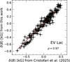 |
Fig. 3 Comparison between δ〈B〉 obtained in this work and the values of Cristofari et al. (2025). The average 〈B〉 was removed from the estimates of Cristofari et al. (2025) for comparison. The red line shows the equality. The Pearson correlation coefficient (ρ) is shown on the figure. Our process allows us to retrieve δ〈B〉 values that are in very good agreement with those obtained from fits of synthetic spectra to the data. |
5.2 Application to ESPaDOnS and Narval spectra
To complete our analysis, we applied our process to optical spectra recorded with Narval and ESPaDOnS for EV Lac and DS Leo (see Sect. 2). The derived relative magnetic field strengths are well modeled by a QPGP (see Figs. 4 and 5), yielding rotation periods of Prot = 4.367 ± 0.023 d and Prot = 14.105 ± 0.406 d for EV Lac and DS Leo, respectively. These estimates are in very good agreement with those reported by Cristofari et al. (2025) of Prot = 4.362 ± 0.001 d and Prot = 13.953 ± 0.088 d, albeit with larger error bars. The larger error bars can partly be attributed to the sparsity of the available Narval and ESPaDOnS data, as a result of the observing strategies primarily focused on Zeeman Doppler Imaging reconstructions (see, e.g., Morin et al. 2008, 2011; Donati et al. 2008; Bellotti et al. 2024). This underscores the benefits of long-term spectroscopic monitoring of M dwarfs, not only for the planet search, but for the study of their magnetic fields as well. We note that DS Leo was reported to exhibit differential rotation, with distinct rotation periods at the equator and the poles (13.37 ± 0.86 d and 14.96 ± 1.25 d, respectively; Hébrard et al. 2016), which could in part account for the larger error bar derived with our GP fit.
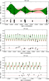 |
Fig. 4 Best QPGP fit (green) obtained on relative small-scale magnetic field estimates derived from ESPaDOnS and Narval spectra for EV Lac. Top panel: fit over the entire dataset. Middle and bottom: segments of the dataset. The residuals (Res.) between data points and GP fit are shown on each panel. |
5.3 Model-driven δ T variations
We applied the model-driven approach used to derive temperature variation (see Sect. 4.3) to the observed spectra considered in our study. For EV Lac (Gl 873) and DS Leo (Gl 410), we find significant correlations between our derived δT and the data-driven estimates obtained with the LBL (Artigau et al. 2024) and published by Cristofari et al. (2025), with Pearson correlation coefficients of 0.95 and 0.93, respectively (see Fig. C.2). A moderate correlation is also observed for Barnard’s star, with a Pearson coefficient of 0.59 (see Fig. C.2). We note the smaller range of the variations relative to error bars for this star. These results demonstrate the ability models have to reproduce relative temperature variations in spite of the significant discrepancies between models and observations (see, e.g., Cristofari et al. 2022b,a). We note that in a similar experiment, Artigau et al. (2024) found that model-driven variations led to a damping of the retrieved δT. Details in implementation and normalization, along with differences between the models used could explain our ability to retrieve amplitudes comparable to those obtained with the data-driven approach. Our results further support previous findings (Bellotti et al. 2025) where synthetic spectra were used to estimate temperature and 〈B〉 variations from spectra recorded with SPIRou.
From the spectra recorded with SPIRou, we observed strong anti-correlations between our δT and δ〈B〉 estimates. We applied orthogonal distance regressions1 (ODRs) to estimate the properties of the linear relationships between δT and δ〈B〉 (see Figs. 6 and D.1). For EV Lac, DS Leo, and Barnard’s star, the fits yield slopes of −18.3 ± 0.6, −54.2 ± 1.8K kG−1, and −24.7 ± 1.0 K kG−1, consistent with those reported by Cristofari et al. (2025, −19.8 ± 0.5, −60.4 ± 2.5, and −18.8 ± 0.8K kG−1, respectively). We note that the ODR is very sensitive to the relative scaling of the error bars of both axes, which can have an impact of several K kG−1 in our case.
From the data recorded with Narval/ESPaDOnS, we can observe similar anticorrelations between δT and δ〈B〉, with significantly larger scatters, yielding slopes of −22.3 ± 3.3 and −61.7 ± 6.8 K kG−1 for EV Lac and DS Leo, respectively. The larger scatters in the results could be attributed to the impact of magnetic fields on δT estimates (see Sect. 4.3), the sparsity of the observations obtained with Narval/ESPaDOnS, or the higher contrast in the optical where cool spots could lead to larger temperature variations which may not be strictly anticorrelated with δB.
We note that while our simulations suggest that the impact of magnetic fields on the derived δT is more significant for the Narval/ESPaDOnS domain, it could still have a non-negligible impact on the estimates obtained from spectra recorded in the nIR, which could lead to steeper slopes and larger scattering. A natural next step would be to use the δ〈B〉 estimates to obtain magnetic field-dependent ∂A/∂T values (see Eq. (4)) and rely on these to refine the δT measurements. We leave the implementation of this process to a future study.
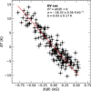 |
Fig. 6 Relation between our model-driven δT and δ〈B〉 estimates obtained from SPIRou data for EV Lac. The red line shows the best linear fit to the data point, obtained with an orthogonal distance regression. The parameters of the fit are shown on the figure. |
5.3.1 Comparison to activity indicators
From Narval and ESPaDOnS spectra, we measured the Sindex, commonly used as an activity proxy, to compare it to our δ〈B〉 estimates. We followed the definition of the S-index from Vaughan et al. (1978):
 (6)
(6)
where FH and FK are the fluxes taken in 1.09 Å triangular bands centered on 3968.470 and 3933.661 Å, respectively. FR and FV are the fluxes computed in 20 Å rectangular bands centered on 3901 and 4001 Å, respectively (see Fig. F.1). The coefficients a, b, c, d, and e, which allow us to calibrate the index to the Mount Wilson scale, were taken from Marsden et al. (2014). The flux uncertainties were propagated to estimate the error bars on each band’s flux, which were, in turn, used to define error bars on the S-index measurements.
We recall here that δ〈B〉 is directly linked to 〈B〉 such that 〈B〉 = δ〈B〉 + 〈B〉ref, with 〈B〉ref the value associated with the reference spectrum (see Eq. (4)). For an easier comparison with the literature, in Fig. 7, we computed 〈B〉 from δ〈B〉, taking the typical 〈B〉ref values from Cristofari et al. (2025) for EV Lac and DS Leo (4.54 and 0.79 kG, respectively). No clear correlation was observed between the measured S-index and the magnetic field strength variation derived with our approach for EV Lac or DS Leo (Fig. 7). We note that the long baseline of the observations (~10 yr) could encompass activity regime changes that could break the activity-〈B〉 relationship that would be expected for an activity driven by quiescent heating. For both stars, we divided the observations in segments of closely spaced observations and compared the activity indicators to δ〈B〉 in these. A tentative correlation (with a Pearson coefficient of 0.57) can be observed for DS Leo if we are only considering data points between BJD 2454400 and 2455700. These dates encompass observation campaigns where the magnetic field strength is at its lowest. These results further suggest that changes in activity regimes could throw off the relation between the S-index and average surface magnetic field strength on long observation baselines. Recently, Hahlin et al. (2026) reported correlations between the S-index and 〈B〉 for a few hotter stars (Teff ranging from ~4350 to 5400 K), suggesting that such a relation might be harder to recover for M dwarfs than it would be for Sun-like stars.
Moreover, DS Leo and EV Lac are known to exhibit flares (e.g., Muheki et al. 2020; Duvvuri et al. 2023) with a direct impact on activity indicators that can throw off the relation between magnetic fields and activity (Getman et al. 2025). Previous work noted that flares can lead to larger X-ray luminosity than expected for a given magnetic flux (Pevtsov et al. 2003; Getman et al. 2025), suggesting that much more energy is released by flares than by quiescent magnetic heating. These flares can impact all outer layers of the stellar atmosphere, consequently enhancing chromospheric emission. These results underscore the importance of average magnetic field measurements, less prone to biases associated with chromospheric activity.
6 Discussion and conclusions
In this paper, we study the temporal behavior of magnetic fields from long-term spectroscopic monitoring of cool stars (see, e.g., Donati et al. 2023a; Cristofari et al. 2025). We explore a simple method to estimate relative variations of small-scale magnetic fields (δ〈B〉) from high-resolution spectra. The proposed method does not rely on fits of synthetic spectra to individual observations, providing extremely fast estimates in comparison.
Studies that rely on fits of synthetic spectra to observations (e.g., Reiners et al. 2022; Cristofari et al. 2025) are inherently limited by the quality of the fits, with systematics between modeled and observed line shapes leading to uncertainties and potential biases in the results. The method proposed in this paper attempts to mitigate these effects by only studying changes in line shapes relative to a reference spectrum, obtained from the observations themselves. While the fundamental idea of studying spectral feature variations compared to a reference spectrum is not new, with notable applications for radial velocity (Artigau et al. 2022) and surface temperature variations (Artigau et al. 2024), this is to our knowledge the first such attempt to derive relative small-scale magnetic field variations (δ〈B〉).
With this work, we show that our model-informed process applied to observations can provide reliable information on δ〈B〉 from series of high-resolution spectra. Our approach relies on synthetic spectra computed with ZeeTurbo (Cristofari et al. 2023a), applied to high-resolution near-infrared and optical spectra recorded with SPIRou, Narval, and ESPaDOnS. Our results were compared to magnetic field measurements previously obtained for a few strongly magnetic targets (Cristofari et al. 2025), yielding an excellent agreement. This underscores the reliability of the process, which (by construction) allows us to obtain δ〈B〉 from a linear fit, instead of expensive MCMC sampling (Cristofari et al. 2025). Consequently, the proposed method enables the treatment of hundreds of spectra in seconds, making it a diagnostic tool that is viable for systematic application to spectra recorded in the context of large surveys to come.
The analysis of Narval and ESPaDOnS spectra provide new constraints on the long-term variations of the small-scale magnetic fields for EV Lac and DS Leo. QPGP fits to the series of δ〈B〉 measurements show a clear modulation consistent with the rotation period of the stars. We note that this has been achieved in spite of the relative sparsity of the data over a ten-year period, compared the dense survey carried out with SPIRou over three years.
Through simulations and analysis of the observed data, we investigated the impact that assumptions on atmospheric properties have on the results and found that our method is relatively resilient with respect to small changes in the adopted parameters. We also found that significant offset in the assumed atmospheric properties leads to a damping of the derived δ〈B〉. Consequently, even with an incorrect stellar characterization, our method provides valuable information on the temporal behavior of the magnetic fields, with a damped amplitude. Our simulations also underscore the importance of careful relative normalization, as short-window median filters tend to impact the shape of broad absorption features, with significant impacts on both δ〈B〉 and temperature variation estimates (δT). The proposed method allows for the retrieval of extremely fast estimates of the absolute surface magnetic field strength (〈B〉) for a series of spectra, provided that the value associated with the reference spectrum is known. Such an initial estimate can be obtained with the methods commonly used to derive field strengths (e.g., Reiners et al. 2022; Cristofari et al. 2023b; Kochukhov et al. 2024).
We implemented a model-driven process following Artigau et al. (2024) to derive relative temperature variations (δT) from the observed spectra. For EV Lac and DS Leo, we found an excellent agreement between our results and the data-driven δT obtained in the framework of the LBL code by (Artigau et al. 2024). Similarly to Cristofari et al. (2025), we find significant anticorrelation between δT and δ〈B〉, suggesting that the observed magnetic fields are directly linked to the presence of cooler spots at the stellar surface. Relying on spectra recorded with ESPaDOnS and Narval, we see clear anticorrelations between our retrieved δT and δ〈B〉 for EV Lac and DS Leo. We obtained similar slopes between δT and δ〈B〉 for the optical and nIR domains, although with a significantly higher scatter in the optical domain. Several competing factors could explain these results, including the possibly higher sensitivity to temperature variations in the optical, caused by higher contrast between spots and the photosphere (Berdyugina 2005). One identified cause, however, could be the influence of magnetic fields on the δT estimates. Simulations revealed that magnetic field variations can lead to an increased scatter and larger amplitudes in the derived δT (Fig. 2), particularly for regions containing a large number of magnetically sensitive transitions, which is consistent with the larger scatter observed for ESPaDOnS and Narval data. We note that a natural next step could be to rely on the δ〈B〉 measurements to refine δT estimates. Using δ〈B〉, we could compute magnetic-field dependent ∂A/∂T (Eq. (4)) and used these to obtain more accurate δT. We leave the detailed implementation of this process to a subsequent study. We note that temperature variations can also have a small impact on the derived δ〈B〉, although these appear small in light of the current measurements precision. The next generation of instruments will provide spectra with much higher quality and the implementation of temperature dependent magnetic models, mimicking the impact of cool magnetic spots at the stellar surface, will enable a more detailed modeling of the stellar spectra.
Narval and ESPaDOnS data provide access to the CaII H&K lines, which we used to measure the S-index, widely used as an activity indicator in Sun-like stars and M dwarfs. We found no clear correlation between the S-index estimates and our δ〈B〉 measurements. These results can largely be attributed to the nature of the activity in M dwarfs, which are more prone to chromospheric activity and flares, potentially throwing off the relation that typically arises from steady quiescent heating. In addition, the relatively low S/N in the blue orders of the ESPaDOnS/Narval spectrograph for M dwarfs can impact our S-index estimates. Observations recorded with these instruments also span close to a decade, while studies looking at the detailed correlation between S-index and 〈B〉 in the Sun typically focused on much smaller timescales. Complex long-term fluctuations in the magnetic activity could throw off the S-index-〈B〉 relation observed in the Sun. These results underscore the need for smallscale magnetic field measurements which are less impacted by chromospheric activity and the need for dense observation campaigns to fully explore the link between surface magnetic fields and activity indicators in low-mass stars.
The current method will benefit from improvement in the models used to obtain the relative variation of pixels with magnetic field strength. The models used in this work were computed under the assumption that only atoms are sensitive to magnetic fields, due to the lack of known Landé factors for most magnetically sensitive molecules. While the impact of magnetically sensitive molecules on the results can be mitigated by pixel rejection strategies and avoiding dense molecular bands, including the impact of magnetic fields on sensitive molecules (such as TiO) will allow for the precision of the proposed method to be improved.
Finally, we find that the proposed method can have significant benefits for the correction of radial velocity curves in the context of exoplanet searches. Recent studies have suggested that 〈B〉 can be an excellent indicator of activity jitters in radial velocity curves (Haywood et al. 2016, 2022). The ability to obtain fast and reliable constraints from the same data used to measure RVs opens the door to new strategies for activity jitter correction for extracting planetary signals from the recorded data.
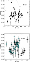 |
Fig. 7 S-index compared to 〈B〉 for EV Lac (top) and DS Leo (bottom). 〈B〉 estimates were obtained from δ〈B〉 by adding typical median values from Cristofari et al. (2025), of 4.54 and 0.79 kG for EV Lac and DS Leo, respectively. For DS Leo, points marked with a cyan circle correspond to observations recorded between BJD 2454400 and 2455700 (see Fig. 5). |
Data availability
The Full appendix Tables are available at the CDS via https://cdsarc.cds.unistra.fr/viz-bin/cat/J/A+A/708/A207.
Acknowledgements
This project has received funding from the European Research Council (ERC) under the European Union’s Horizon 2020 research and innovation programme (grant agreement No. 817540, ASTROFLOW). This project has received funding from the Dutch Research Council (NWO), with project numbers VI.C.232.041 of the Talent Programme Vici and OCENW.M.22.215 of the research programme “Open Competition Domain Science - M”. S.H.S. gratefully acknowledges support from NASA EPRV grant 80NSSC21K1037, NASA XRP grant 80NSSC21K0607, and NASA Heliophysics LWS grant NNX16AB79G.
References
- Angus, R., Morton, T., Aigrain, S., Foreman-Mackey, D., & Rajpaul, V. 2018, MNRAS, 474, 2094 [Google Scholar]
- Artigau, É., Cadieux, C., Cook, N. J., et al. 2022, AJ, 164, 84 [NASA ADS] [CrossRef] [Google Scholar]
- Artigau, É., Cadieux, C., Cook, N. J., et al. 2024, AJ, 168, 252 [Google Scholar]
- Bellotti, S., Petit, P., Morin, J., et al. 2022, A&A, 657, A107 [NASA ADS] [CrossRef] [EDP Sciences] [Google Scholar]
- Bellotti, S., Morin, J., Lehmann, L. T., et al. 2024, A&A, 686, A66 [NASA ADS] [CrossRef] [EDP Sciences] [Google Scholar]
- Bellotti, S., Cristofari, P. I., Callingham, J. R., et al. 2025, A&A, 704, A298 [NASA ADS] [CrossRef] [EDP Sciences] [Google Scholar]
- Berdyugina, S. V. 2005, Living Rev. Sol. Phys., 2, 8 [Google Scholar]
- Bonfils, X., Lo Curto, G., Correia, A. C. M., et al. 2013, A&A, 556, A110 [NASA ADS] [CrossRef] [EDP Sciences] [Google Scholar]
- Bouchy, F., Pepe, F., & Queloz, D. 2001, A&A, 374, 733 [NASA ADS] [CrossRef] [EDP Sciences] [Google Scholar]
- Chabrier, G., & Baraffe, I. 1997, Structure and Evolution of Low-Mass Stars [Google Scholar]
- Chabrier, G., & Küker, M. 2006, A&A, 446, 1027 [NASA ADS] [CrossRef] [EDP Sciences] [Google Scholar]
- Charbonneau, P. 2010, Living Rev. Sol. Phys., 7, 3 [NASA ADS] [CrossRef] [Google Scholar]
- Cook, N. J., Artigau, É., Doyon, R., et al. 2022, PASP, 134, 114509 [NASA ADS] [CrossRef] [Google Scholar]
- Cristofari, P. I., Donati, J.-F., Masseron, T., et al. 2022a, MNRAS, 516, 3802 [NASA ADS] [CrossRef] [Google Scholar]
- Cristofari, P. I., Donati, J.-F., Masseron, T., et al. 2022b, MNRAS, 511, 1893 [NASA ADS] [CrossRef] [Google Scholar]
- Cristofari, P. I., Donati, J.-F., Folsom, C. P., et al. 2023a, MNRAS, 522, 1342 [NASA ADS] [CrossRef] [Google Scholar]
- Cristofari, P. I., Donati, J.-F., Moutou, C., et al. 2023b, MNRAS, 526, 5648 [NASA ADS] [CrossRef] [Google Scholar]
- Cristofari, P. I., Donati, J.-F., Bellotti, S., et al. 2025, A&A, 702, A111 [NASA ADS] [CrossRef] [EDP Sciences] [Google Scholar]
- Donati, J.-F. 2003, in Astronomical Society of the Pacific Conference Series, 307, Solar Polarization, eds. J. Trujillo-Bueno, & J. Sanchez Almeida, 41 [Google Scholar]
- Donati, J.-F., & Landstreet, J. D. 2009, ARA&A, 47, 333 [Google Scholar]
- Donati, J.-F., Semel, M., Carter, B. D., Rees, D. E., & Cameron, A. C. 1997, MNRAS, 291, 658 [Google Scholar]
- Donati, J. F., Catala, C., Landstreet, J. D., & Petit, P. 2006, in Astronomical Society of the Pacific Conference Series, 358, Solar Polarization 4, eds. R. Casini, & B. W. Lites, 362 [Google Scholar]
- Donati, J.-F., Morin, J., Petit, P., et al. 2008, MNRAS, 390, 545 [NASA ADS] [CrossRef] [Google Scholar]
- Donati, J.-F., Kouach, D., Moutou, C., et al. 2020, MNRAS, 498, 5684 [NASA ADS] [CrossRef] [Google Scholar]
- Donati, J.-F., Cristofari, P. I., Finociety, B., et al. 2023a, MNRAS, 525, 455 [NASA ADS] [CrossRef] [Google Scholar]
- Donati, J.-F., Lehmann, L. T., Cristofari, P. I., et al. 2023b, MNRAS, 525, 2015 [CrossRef] [Google Scholar]
- Donati, J.-F., Gaidos, E., Moutou, C., et al. 2025, A&A, 698, L14 [NASA ADS] [CrossRef] [EDP Sciences] [Google Scholar]
- Dorn, R. J., Bristow, P., Smoker, J. V., et al. 2023, A&A, 671, A24 [NASA ADS] [CrossRef] [EDP Sciences] [Google Scholar]
- Dressing, C. D., & Charbonneau, D. 2015, ApJ, 807, 45 [Google Scholar]
- Dumusque, X., Cretignier, M., Sosnowska, D., et al. 2021, A&A, 648, A103 [NASA ADS] [CrossRef] [EDP Sciences] [Google Scholar]
- Duvvuri, G. M., Pineda, J. S., Berta-Thompson, Z. K., France, K., & Youngblood, A. 2023, AJ, 165, 12 [Google Scholar]
- Finociety, B., Donati, J.-F., Cristofari, P. I., et al. 2023, MNRAS, 526, 4627 [NASA ADS] [CrossRef] [Google Scholar]
- Fouqué, P., Martioli, E., Donati, J.-F., et al. 2023, A&A, 672, A52 [NASA ADS] [CrossRef] [EDP Sciences] [Google Scholar]
- Gaidos, E., Mann, A. W., Kraus, A. L., & Ireland, M. 2016, MNRAS, 457, 2877 [Google Scholar]
- Getman, K. V., Kochukhov, O., Ninan, J. P., et al. 2025, ApJ, 980, 57 [Google Scholar]
- Gray, D. F. 1994, PASP, 106, 1248 [NASA ADS] [CrossRef] [Google Scholar]
- Gray, D. F., & Johanson, H. L. 1991, PASP, 103, 439 [NASA ADS] [CrossRef] [Google Scholar]
- Hahlin, A., Zaire, B., Folsom, C. P., Al Moulla, K., & Lavail, A. 2026, A&A, 706, A138 [NASA ADS] [CrossRef] [EDP Sciences] [Google Scholar]
- Haywood, R. D., Collier Cameron, A., Unruh, Y. C., et al. 2016, MNRAS, 457, 3637 [Google Scholar]
- Haywood, R. D., Milbourne, T. W., Saar, S. H., et al. 2022, ApJ, 935, 6 [NASA ADS] [CrossRef] [Google Scholar]
- Hébrard, É. M., Donati, J.-F., Delfosse, X., et al. 2016, MNRAS, 461, 1465 [CrossRef] [Google Scholar]
- Johns-Krull, C. M., & Valenti, J. A. 1996, ApJ, 459, L95 [NASA ADS] [Google Scholar]
- Kochukhov, O. 2021, A&A Rev., 29, 1 [Google Scholar]
- Kochukhov, O., & Lavail, A. 2017, ApJ, 835, L4 [Google Scholar]
- Kochukhov, O., & Reiners, A. 2020, ApJ, 902, 43 [Google Scholar]
- Kochukhov, O., Amarsi, A. M., Lavail, A., et al. 2024, A&A, 689, A36 [NASA ADS] [CrossRef] [EDP Sciences] [Google Scholar]
- Marsden, S. C., Petit, P., Jeffers, S. V., et al. 2014, MNRAS, 444, 3517 [Google Scholar]
- Morin, J., Donati, J.-F., Petit, P., et al. 2008, MNRAS, 390, 567 [Google Scholar]
- Morin, J., Dormy, E., Schrinner, M., & Donati, J.-F. 2011, MNRAS, 418, L133 [CrossRef] [Google Scholar]
- Muheki, P., Guenther, E. W., Mutabazi, T., & Jurua, E. 2020, MNRAS, 499, 5047 [NASA ADS] [CrossRef] [Google Scholar]
- Parker, E. N. 1955, ApJ, 122, 293 [Google Scholar]
- Pecaut, M. J., & Mamajek, E. E. 2013, ApJS, 208, 9 [Google Scholar]
- Petit, P., Louge, T., Théado, S., et al. 2014, PASP, 126, 469 [NASA ADS] [CrossRef] [Google Scholar]
- Pevtsov, A. A., Fisher, G. H., Acton, L. W., et al. 2003, ApJ, 598, 1387 [Google Scholar]
- Quirrenbach, A., Amado, P. J., Caballero, J. A., et al. 2014, SPIE Conf. Ser., 9147, 91471F [Google Scholar]
- Reiners, A., Shulyak, D., Käpylä, P. J., et al. 2022, A&A, 662, A41 [NASA ADS] [CrossRef] [EDP Sciences] [Google Scholar]
- Reylé, C., Jardine, K., Fouqué, P., et al. 2021, A&A, 650, A201 [Google Scholar]
- Saar, S. H., & Linsky, J. L. 1985, ApJ, 299, L47 [Google Scholar]
- Shahaf, S., & Zackay, B. 2023, MNRAS, 525, 6223 [NASA ADS] [CrossRef] [Google Scholar]
- Shulyak, D., Reiners, A., Seemann, U., Kochukhov, O., & Piskunov, N. 2014, A&A, 563, A35 [NASA ADS] [CrossRef] [EDP Sciences] [Google Scholar]
- Shulyak, D., Reiners, A., Engeln, A., et al. 2017, Nat. Astron., 1, 0184 [NASA ADS] [CrossRef] [Google Scholar]
- Shulyak, D., Reiners, A., Nagel, E., et al. 2019, A&A, 626, A86 [NASA ADS] [CrossRef] [EDP Sciences] [Google Scholar]
- Skumanich, A. 1972, ApJ, 171, 565 [Google Scholar]
- Spiegel, E. A., & Zahn, J.-P. 1992, A&A, 265, 106 [Google Scholar]
- Vaughan, A. H., Preston, G. W., & Wilson, O. C. 1978, PASP, 90, 267 [Google Scholar]
- Vidotto, A. A., Gregory, S. G., Jardine, M., et al. 2014, MNRAS, 441, 2361 [Google Scholar]
- Virtanen, P., Gommers, R., Oliphant, T. E., et al. 2020, Nat. Methods, 17, 261 [Google Scholar]
- Yadav, R. K., Christensen, U. R., Morin, J., et al. 2015, ApJ, 813, L31 [Google Scholar]
Implementation relying on Scipy (Virtanen et al. 2020).
Appendix A Data tables
Tables A.1, A.2, and A.3 report our δ〈B〉 and δT measurements obtained from spectra recorded with SPIRou for EV Lac, DS Leo and Barnard’s star, respectively. Tables A.4 and A.5 present similar data obtained from spectra recorded with Narval/ESPaDOnS for EV Lac and DS Leo, respectively.
δ〈B〉 and δT measurements obtained for EV Lac from spectra recorded with SPIRou.
δ〈B〉 and δT measurements obtained for EV Lac from spectra recorded with Narval/ESPaDOnS (extract).
Appendix B GP fit parameters
Table B.1 presents the GP parameters retrieved from posterior distribution by applying our process to the spectra recorded with SPIRou. Table B.2 presents the same parameters obtained by applying our process to the spectra recorded with Nar-val/ESPaDOnS.
Appendix C Additional comparisons
Figure C.1 presents the comparison between δ〈B〉 obtained in this paper, and those of Cristofari et al. (2025). Figure C.2 presents comparisons between the retrieved δT and the model-driven variations obtained with the LBL.
GP hyper-parameters obtained for EV Lac, DS Leo, and Barnard’s star from SPIRou spectra.
Appendix D δ〈B〉 - δT relations
Figure D.1 presents the comparison between our derived δ〈B〉 and model-driven δT obtained from SPIRou spectra for DS Leo and Barnard’s star. Figure D.2 presents similar comparisons for the estimates obtained from Narval/ESPaDOnS data, for EV Lac and DS Leo.
Appendix E Corner plots
Figures E.1, E.2, and E.3 present the corner plots showing the posterior distributions of the hyper-parameters associated with the quasi-periodic Gaussian Fit on δ〈B〉 estimates obtained from SPIRou spectra for EV Lac, DS Leo and Barnard’s star, respectively. Figures E.4 and E.5 present similar corner plots obtained with δ〈B〉 estimates derived from Narval/ESPaDOnS spectra for EV Lac and DS Leo, respectively.
GP hyper-parameters obtained for EV Lac and DS Leo from Narval/ESPaDOnS spectra.
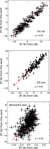 |
Fig. C.2 Comparison between our model-driven δT and the data-driven estimates obtained with the LBL (see Artigau et al. 2024; Cristofari et al. 2025) for EV Lac (top panel), DS Leo (middle panel), and Barnard’s star (bottom panel). The red line shows the equality. |
Appendix F S-index calculation
Figure F.1 shows an example of spectrum showing the bands used to compute the S-index.
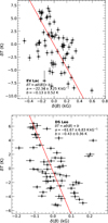 |
Fig. D.2 Relation between our model δT and δ〈B〉 estimates obtained from Narval/ESPaDOnS data for EV Lac (top panel) and DS Leo (bottom panel). The red line shows the best linear fits obtained with an orthogonal distance regression. The parameters of the fits are shown on the figure. |
 |
Fig. E.1 Posterior distribution walkers for the GP parameters obtained on δ〈B〉 extracted from the spectra recorded with SPIRou for EV Lac. |
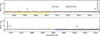 |
Fig. F.1 Example of spectrum obtained with Narval, showing the V and R rectangular bands, along with the K and H triangular bands used to compute the S-index. |
All Tables
δ〈B〉 and δT measurements obtained for EV Lac from spectra recorded with SPIRou.
δ〈B〉 and δT measurements obtained for EV Lac from spectra recorded with Narval/ESPaDOnS (extract).
GP hyper-parameters obtained for EV Lac, DS Leo, and Barnard’s star from SPIRou spectra.
GP hyper-parameters obtained for EV Lac and DS Leo from Narval/ESPaDOnS spectra.
All Figures
|
Fig. 1 Comparison between the retrieved (y-axis) and input (x-axis) relative magnetic field strengths (δ〈B〉). The synthetic observations were normalized to the template using a rolling median with a window of 100km s−1. The red squares and green plus symbols (‘+’) show the results obtained before and after re-normalizing the models used to computed Fk - F0 (Eq. (4)) with a 100 km s−1 median filter, respectively (see text). The black line marks the equality. This figure illustrates the need for careful re-normalization of the models to avoid biases in the results. |
| In the text | |
|
Fig. 2 Comparison between the retrieved δT (y-axis) and the input δT used to generate the synthetic observations (x-axis). Synthetic observations were computed on the wavelength range covered by Narval/ESPaDOnS, accounting for magnetic field variations (red squares), or fixing the value of the magnetic fields to 0 kG (green circles). This figure illustrates how magnetic fields can impact the δT estimates. |
| In the text | |
|
Fig. 3 Comparison between δ〈B〉 obtained in this work and the values of Cristofari et al. (2025). The average 〈B〉 was removed from the estimates of Cristofari et al. (2025) for comparison. The red line shows the equality. The Pearson correlation coefficient (ρ) is shown on the figure. Our process allows us to retrieve δ〈B〉 values that are in very good agreement with those obtained from fits of synthetic spectra to the data. |
| In the text | |
|
Fig. 4 Best QPGP fit (green) obtained on relative small-scale magnetic field estimates derived from ESPaDOnS and Narval spectra for EV Lac. Top panel: fit over the entire dataset. Middle and bottom: segments of the dataset. The residuals (Res.) between data points and GP fit are shown on each panel. |
| In the text | |
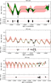 |
Fig. 5 Same as Fig. 4, but for DS Leo. |
| In the text | |
|
Fig. 6 Relation between our model-driven δT and δ〈B〉 estimates obtained from SPIRou data for EV Lac. The red line shows the best linear fit to the data point, obtained with an orthogonal distance regression. The parameters of the fit are shown on the figure. |
| In the text | |
|
Fig. 7 S-index compared to 〈B〉 for EV Lac (top) and DS Leo (bottom). 〈B〉 estimates were obtained from δ〈B〉 by adding typical median values from Cristofari et al. (2025), of 4.54 and 0.79 kG for EV Lac and DS Leo, respectively. For DS Leo, points marked with a cyan circle correspond to observations recorded between BJD 2454400 and 2455700 (see Fig. 5). |
| In the text | |
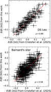 |
Fig. C.1 Same as Fig. 3, but for DS Leo (top panel) and Barnard’s star (bottom panel). |
| In the text | |
|
Fig. C.2 Comparison between our model-driven δT and the data-driven estimates obtained with the LBL (see Artigau et al. 2024; Cristofari et al. 2025) for EV Lac (top panel), DS Leo (middle panel), and Barnard’s star (bottom panel). The red line shows the equality. |
| In the text | |
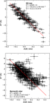 |
Fig. D.1 Same as Fig. 6 but for DS Leo (top panel) and Barnard’s star (bottom panel). |
| In the text | |
|
Fig. D.2 Relation between our model δT and δ〈B〉 estimates obtained from Narval/ESPaDOnS data for EV Lac (top panel) and DS Leo (bottom panel). The red line shows the best linear fits obtained with an orthogonal distance regression. The parameters of the fits are shown on the figure. |
| In the text | |
|
Fig. E.1 Posterior distribution walkers for the GP parameters obtained on δ〈B〉 extracted from the spectra recorded with SPIRou for EV Lac. |
| In the text | |
 |
Fig. E.2 Same as Fig. E.1, but for DS Leo. |
| In the text | |
 |
Fig. E.3 Same as Fig. E.1, but for Barnard’s star. |
| In the text | |
 |
Fig. E.4 Same as Fig. E.1, but for EV Lac from data recorded with Narval/ESPaDOnS. |
| In the text | |
 |
Fig. E.5 Same as Fig. E.1, but for DS Leo from data recorded with Narval/ESPaDOnS. |
| In the text | |
|
Fig. F.1 Example of spectrum obtained with Narval, showing the V and R rectangular bands, along with the K and H triangular bands used to compute the S-index. |
| In the text | |
Current usage metrics show cumulative count of Article Views (full-text article views including HTML views, PDF and ePub downloads, according to the available data) and Abstracts Views on Vision4Press platform.
Data correspond to usage on the plateform after 2015. The current usage metrics is available 48-96 hours after online publication and is updated daily on week days.
Initial download of the metrics may take a while.