| Issue |
A&A
Volume 708, April 2026
|
|
|---|---|---|
| Article Number | A183 | |
| Number of page(s) | 9 | |
| Section | Planets, planetary systems, and small bodies | |
| DOI | https://doi.org/10.1051/0004-6361/202658944 | |
| Published online | 09 April 2026 | |
TOI-1333Ab is on a well-aligned orbit
An aligned hot Jupiter around an F-type star with a mutually inclined stellar companion
1
Stellar Astrophysics Centre, Department of Physics and Astronomy, Aarhus University,
Ny Munkegade 120,
8000
Aarhus C,
Denmark
2
Department of Space, Earth and Environment, Chalmers University of Technology,
412 93,
Gothenburg,
Sweden
3
Department of Space, Earth and Environment, Chalmers University of Technology, Onsala Space Observatory,
439 92
Onsala,
Sweden
★ Corresponding author: This email address is being protected from spambots. You need JavaScript enabled to view it.
Received:
13
January
2026
Accepted:
6
March
2026
Abstract
Context. Spin-orbit obliquity measurements of hot-Jupiter systems constrain giant planet migration and tidal evolution. In binary systems, combining stellar obliquities with the orbit-orbit angle (γ) between the planetary and stellar companion orbits provides further insight into the dynamical influence of stellar companions.
Aims. Here we aim to determine the projected obliquity (λ) of the hot Jupiter TOI-1333Ab (P ≈ 4.72 d, Mp ≈ 2.4 MJ) and place the system in the context of hot-Jupiter migration and tidal realignment in binary systems.
Methods. We analysed spectroscopic observations obtained during planetary transit to model the Rossiter-McLaughlin effect and derive the projected obliquity. We combined this measurement with published system parameters and constraints on the wide stellar companion orbit to assess plausible migration scenarios.
Results. We measure a projected obliquity of λ =-5 ± 10°, showing that TOI-1333Ab is well aligned with the stellar spin axis of its F-type host star. The low obliquity and its modest eccentricity (e = 0.073−0.052+0.092) are consistent with either disc-driven migration or high-eccentricity migration followed by efficient tidal circularisation and realignment. With an effective temperature of 6274 ± 97 K, the host star lies above the canonical Kraft break where the systems are frequently misaligned. Despite this, we find the system to be well aligned. In comparison with other planetary systems in binaries, TOI-1333 occupies a relatively isolated region in projected obliquity-orbit-orbit angle (γ = 81.5 ± 1.1°) space, making it a valuable system for studying the interplay between migration, tides, and stellar companions.
Key words: planets and satellites: dynamical evolution and stability / planets and satellites: gaseous planets / planet-star interactions
© The Authors 2026
 Open Access article, published by EDP Sciences, under the terms of the Creative Commons Attribution License (https://creativecommons.org/licenses/by/4.0), which permits unrestricted use, distribution, and reproduction in any medium, provided the original work is properly cited.
This article is published in open access under the Subscribe to Open model. This email address is being protected from spambots. You need JavaScript enabled to view it. to support open access publication.
1 Introduction
When it comes to gauging the processes at work in forming and shaping exoplanet systems, measurements of the relative orientation between the stellar spin axes and planetary orbital planes offer a powerful diagnostic. While planets formed within protoplanetary discs are expected to begin on well-aligned and nearly circular orbits, subsequent dynamical interactions can significantly alter these configurations (e.g. Biddle et al. 2025). Measurements of the projected spin-orbit angle (obliquity, λ) for hot-Jupiter systems have revealed a striking diversity, ranging from well-aligned systems to polar and retrograde orbits (see Albrecht et al. 2022 for a recent review). This diversity of configurations challenges simple migration scenarios and points towards a combination of dynamical pathways and tidal evolution (a prime example being the hot-Jupiter progenitor TIC 241249530 b; Gupta et al. 2024).
Stellar multiplicity adds an additional layer of complexity to this picture. Wide stellar companions can induce secular perturbations that excite orbital eccentricities and inclinations, potentially triggering high-eccentricity (high-e) migration (e.g. Wu & Murray 2003; Fabrycky & Tremaine 2007). At the same time, tidal interactions between close-in giant planets and their host stars may act to circularise orbits and damp stellar obliquities, with efficiencies that depend sensitively on stellar structure, orbital separation, and planetary mass. Recent observational efforts, aided by large-scale astrometric surveys such as the Gaia mission (Gaia Collaboration 2016), have enabled the characterisation of stellar companion orbits and orbit-orbit angles in hot-Jupiter systems, providing new insights into the relationship between stellar multiplicity, spin-orbit misalignment, and planetary system architecture (e.g. Rice et al. 2024).
Through the detection of the Rossiter-McLaughlin (RM; Rossiter 1924; McLaughlin 1924) effect, we present a measurement of the projected obliquity of the TOI-1333A hot-Jupiter system discovered by Rodriguez et al. (2021), hereafter R21. The TOI-1333 system is an S-type binary consisting of the bright (VT = 9.487 ± 0.021; Høg et al. 2000) and evolved primary F-type star, TOI-1333A, and a K-dwarf companion separated at around 560 AU (Michel & Mugrauer 2024). The wide stellar companion, together with its close-in massive planet, makes TOI-1333 an especially valuable system for probing the interplay between giant planet migration, stellar multiplicity, and tidal evolution.
Literature parameters for the TOI-1333A system.
2 Observations
In our analysis to measure the projected obliquity, we combine both photometric and spectroscopic observations, which we detail below. To measure the orbit-orbit angle we use data from Gaia data release 3 (DR3; Gaia Collaboration 2023).
2.1 Photometry
The system was observed by the Transiting Exoplanet Survey Satellite (TESS; Ricker et al. 2015) in Sectors 15, 16, 56, and 76. R21 confirmed and characterised the planet TOI-1333Ab using data from Sectors 15 and 16 along with ground-based photometry, spectroscopy, and imaging. In Table 1, we summarise their findings of this hot-Jupiter system. We downloaded the TESS photometry using the lightkurve package (Lightkurve Collaboration 2018). Sectors 15 and 16 were observed with a cadence of 30 min, and 20-second cadence data are available from Sectors 56 and 76. However, for the latter two sectors we opted for 2-minute cadence data, as both the transit duration was long enough and the number of transits large enough to well sample the transit and describe its shape well. Opting for 2-minute cadence data has the advantage of limiting computation time when calculating light curves. Additionally, a ‘blue noise’ component has been reported in the 20 s cadence data (Kálmán et al. 2025).
After downloading the data, we detrended the light curves using Gaussian process (GP) regression (Rasmussen & Williams 2006) through the celerite library (Foreman-Mackey et al. 2017), making use of the Matérn-3/2 kernel. Detrending was done in an iterative process (three iterations) consisting of four steps: (i) We first temporarily removed the transits using the batman package (Kreidberg 2015) starting with parameters from R21. (ii) We then applied the GP to the transit-free light curves fitting the hyperparameters on a sector-to-sector basis. (iii) We re-injected the transits and cut out snippets of the light curve around the mid-transit points, including four hours of pre-ingress and post-egress data. (iv) Lastly, we performed a complete analysis (see Section 3) to obtain new parameters. The phase-folded light curve is shown in Figure 1. In Figure B.2, we show the transit-free light curve along with the GP used for detrending.
In our analysis, we chose not to include the ground-based photometry presented in R21. Instead, we only include the spacebased photometry from TESS. As the TESS data cover 15 full and four partial transits, the four ground-based transits (three separate and some only partial) do not add much information. One benefit of including the ground-based photometry could be more accurate deblending from contaminant sources in the TESS apertures, as pointed out by Han et al. (2025). They found that the TESS photometry used in R21 might have been overcorrected for contamination, resulting in a planet-to-star radius ratio that is 5.4 ± 3.5% larger in R21. We find a value of  , which is 3 ± 3% larger than - and therefore also consistent with - the value reported in Han et al. (2025). The discrepancy between our value for Rp/R* and that in R21 might also be a product of the two additional TESS sectors we include.
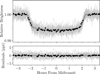 |
Fig. 1 TESS light curve of TOI-1333 folded on the transit of TOI-1333Ab. The black dots demarcate observations taken with a cadence of 30 min. The grey points indicate the 2 min. cadence data. The bestfitting transit model is shown as the solid white line, and the residuals (in parts per thousand) are shown in the bottom. |
2.2 Spectroscopy
We observed a transit of TOI-1333Ab on the night of 12-082025. We made use of the FIES spectrograph (Telting et al. 2014) mounted on the Nordic Optical Telescope (NOT; Djupvik & Andersen 2010). We collected 24 exposures - of which 15 were acquired in transit - each with an exposure time of 900 s, resulting in a signal-to-noise ratio of around 66 (per pixel at 5500 Â). We extracted the radial velocities (RVs) with a custom implementation of the approach outlined in Zechmeister et al. (2018). The median uncertainty is 13 m s−1 with a root mean square of 10 m s−1. The observations are shown in Figure 2, where the RM effect is clearly detected. The FIES RVs are tabulated in Table B.1.
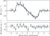 |
Fig. 2 FIES RVs of TOI-1333A after subtracting the best-fitting Keplerian. The solid line denotes the best-fitting model for the RM effect, and the shaded areas represent the 1- and 2-σ confidence intervals. |
3 Data analysis
We are interested in measuring two angles: the angle between the stellar spin axis of TOI-1333A and the orbital axis of TOI-1333Ab (the projected obliquity, λ), and the angle between the planet’s orbit and the binary companion’s orbit (the orbit-orbit angle, γ). In Section A, we discuss the strong rotational modulation seen in the light curve. Should the signal originate from TOI-1333A, the stellar inclination would be  , and the 3D obliquity would be ψ = 40 ± 4°. We are, however, not convinced that TOI-1333A is the source of the rotational modulation, mainly because of strong blending from a nearby bright star. We therefore do not claim a measurement for ψ.
3.1 Projected obliquity
Our approach to extract the projected obliquity is very similar to that outlined in Knudstrup & Albrecht (2022), and we summarise it here. To determine the best-fitting parameters and their uncertainties, we performed Markov chain Monte Carlo (MCMC) sampling using the emcee package (Foreman-Mackey et al. 2013). We modelled the photometric and spectroscopic data jointly to properly account for correlations between parameters such as the impact parameter (b) and λ. This also serves to propagate uncertainties in the mid-transit time (T0) and orbital period (P).
To model the light curves, we used the batman package, which is based on the equations in Mandel & Agol (2002). We used a quadratic limb-darkening law with coefficients (q1, q2) from the tables by Claret et al. (2013); Claret (2018) for the appropriate filters. We stepped in the sum of the limb-darkening coefficients (q1 + q2), applying a Gaussian prior to this value with a width of 0.1, while keeping the difference (q1 - q2) fixed at the tabulated values. The same approach for limb-darkening was applied for the spectroscopic data.
We modelled the RM effect using the framework by Hirano et al. (2011). We included the effects from macro- (Z) and microturbulence (ξ) using the relations by Doyle et al. (2014) and Bruntt et al. (2010), respectively. We adopted these values as Gaussian priors with a width of 1 km s−1. We also included the instrumental dispersion from FIES, which at a resolution of R ~ 67 000 comes out to σPSF = 1.9 km s−1. Thus, in addition to broadening from macro-turbulence, the net Gaussian broadening included in our RM model was  .
.
We applied a uniform prior to the velocity semi-amplitude (K) to account for the fact that the RV slope observed on a given night could differ (from the value from R21) due to stellar variability on a timescale of hours. Given the very modest eccentricity of  reported by R21, we fixed this value to 0.
When running our MCMC, we initialised 100 walkers in a ‘tight Gaussian ball’ around the parameters from R21 - when available. Convergence was assessed by computing the ratio between the length of the chains to the autocorrelation time as well as by visually inspecting the chains and correlation plots. The ratio in our final run came out to more than 300, an indication that the MCMC had converged. In Table 2 we list some of the key parameters from our MCMC, and in Figure 2 and Figure 1 we show the best-fitting models for the RM effect and the light curve, respectively. In Table B.2 we list the posterior values for the full set of parameters along with the priors applied. A correlation plot between λ, b, and v sin i can be found in Figure B.1. Our final result for the projected obliquity is λ = -5 ± 10°.
Key parameters for the TOI-1333A system.
3.2 Orbit-orbit angle
As mentioned, TOI-1333A is part of a binary system; therefore, in addition to the spin-orbit angle we derived the orbit-orbit angle, γ, which is the minimum mutual inclination between the planetary and stellar companion orbits. It is defined as
 (1)
(1)
where r ≡ [∆α, ∆δ] and v ≡ [Aμα*, ∆μδ] are the relative sky-projected position and velocity vectors. Values of γ = 0° or 180° imply that the orbital angular momentum vectors of the planetary and stellar companion orbits are (anti-)aligned, which, for a transiting planet, correspond to the stellar companion orbit being viewed close to edge-on. In contrast, γ ≈ 90° indicates that the stellar companion orbit is nearly perpendicular to the planetary orbit and therefore viewed close to face-on.
Using Gaia DR3 astrometry and following the approach outlined in Section 2.4 of Rice et al. (2024; but see also Behmard et al. 2022), we calculated the orbit-orbit angle. This was done by sampling the astrometric parameters of the primary and secondary stars while accounting for parameter covariances and boundary effects at γ = 0° and 180°. From this, we obtain γ =81.5 ± 1.1°, indicating that we see the orbit almost completely face-on. This is consistent with the analysis from R21 who find the orbital inclination to be  , thereby ruling out an edge-on orbit for the binary.
4 Discussion
Our result for the projected obliquity of -5 ± 10° suggests that TOI-1333A is well aligned with respect to the orbit of TOI-1333Ab. In the context of giant planet migration scenarios, disc migration offers a straightforward explanation for the observed λ, as it has traditionally been considered a more quiet form of migration that produces well-aligned, near-circular orbits (e.g. Lin et al. 1996). This would also explain the very modest eccentricity reported by R21 of  .
.
Another scenario is that the planet migrated via high-e migration through von Zeipel-Kozai-Lidov (ZKL; von Zeipel 1910; Kozai 1962; Lidov 1962) oscillations. In this process a stellar perturber in an orbital plane that is significantly inclined with respect to its planet-(primary) star system can excite the eccentricity of the proto-hot Jupiter through secular interactions (e.g. Wu & Murray 2003). An inclined 1-M⊙ companion at 1000 AU could, for instance, cause ZKL oscillations for a Jupiter-mass planet at 5 AU on a 20 Myr timescale (Fabrycky & Tremaine 2007). In this context, the stellar companion, TOI-13 3 3B, with a mass of M = 0.843 M⊙ and a (sky-projected) separation of 560 AU (Michel & Mugrauer 2024) might have played a relevant part in shaping the architecture of the planetary system, similar to how the companions in TIC 241249530 and HD 80606 (Naef et al. 2001 ; Hébrard et al. 2010) have been hypothesised to excite the eccentricity (and obliquity) in these systems.
The orbital energy from the eccentric (and still wide) orbit of the proto-hot Jupiter could then be removed by tidal dissipation in the planet (Fabrycky & Tremaine 2007), which would both shrink and circularise the orbit. If tidal dissipation is at work, the initial periastron distance would be around 0.03 AU ( AU) with a circularisation timescale comparable to the age (
 Gyr) of the system (Socrates et al. 2012).
In addition to the eccentricity, we might also expect the (projected) obliquity to have been excited dring high-e migration (e.g. Fabrycky & Tremaine 2007). Just as tides (raised on the planet) could have circularised the orbit, tides raised on the star by the planet might have re-aligned it (e.g. Winn et al. 2010; Albrecht et al. 2012). Tidal alignment depends strongly on orbital separation as well as planetary mass, or rather the planet-to-star mass ratio (q). Given the close proximity (a/R* =  ) and mass of the planet (Mp = 2.37 ± 0.24 MJ, q ~ 0.0015 ~ 1.6 ×
  ), TOI-1333A is a system where we expect strong tidal interactions to occur, and we do indeed find it to be a well-aligned system.
However, the tidal realignment timescale has also been hypothesised to depend strongly on stellar structure and may be connected to the location of the Kraft break - a decrease in the rotation rate of mid-F spectral types seen at an effective temperature of Teff ~ 6500 K (Beyer & White 2024). Based on the distribution of the observed projected obliquities, this boundary has typically been placed in the range 6100 K to 6250 K, where stars (hosting hot Jupiters) above this threshold are more frequently found to be misaligned. With an effective temperature of 6274 ± 97 K, TOI-13 3 3A falls in the frequently misaligned regime but with a low projected obliquity.
A recent study published by Wang et al. (2026) statistically delineates the location of the Kraft break, or more accurately, the transition in Teff, where hot-Jupiter systems are more frequently found to be misaligned. Wang et al. (2026) found that by dividing the hot-Jupiter systems (with λ measurements) into either single star systems or binary (or multiple) star systems, the location of the transition for single star systems is very close to the actual Kraft break with  K. On the other hand, the transition occurs at
  K for binaries, and thus closer to the canonical value used for obliquities.
Wang et al. (2026) discuss potential biases for this observed shift towards lower temperatures for the Kraft break among binary systems; one is dilution from the (typically) cooler companion, which shifts the Teff of the host star towards lower temperatures. In the case of TOI-1333, such dilution would bias the inferred Teff of the host star towards lower values, implying that the true effective temperature of TOI-1333A could be higher than the 6274 ± 97 K reported by R21. However, this value resulted from a multi-component fit to the spectral energy distribution (SED), which explicitly should account for this dilution. In addition, the SED fit was constrained by a spectroscopic estimate of Teff = 6250 ± 250 K obtained with the SPC pipeline (Buchhave et al. 2012) from TRES spectra (Fűrész 2008). Given the wide projected separation of the companion (~ 2.8″), dilution is not expected to affect the spectroscopic analysis. We therefore consider the effective temperature of TOI-1333A to be firmly in the hot-star regime. TOI-1333A thus joins a group of well-aligned binary systems with hot(ter) stars, again indicating that multiple factors (such as a/R* and Mp) are at work in sculpting the orbit.
In any case, binary companions to the host stars might play a central role both as triggers for high-e migration and in the efficiency of the subsequent tidal realignment. When examining the orbit-orbit angle for 20 hot Jupiter, multi-star systems with projected obliquity measurements, Behmard et al. (2022) found a tendency for systems with a misaligned host star (λ > 30°) to preferentially occur in face-on (40 < γ < 140°) configurations, suggesting a misalignment with the companion star as well. Contrasting this, Rice et al. (2024) built a larger sample of λ, γ systems and found no such correlation between spin-orbit and orbit-orbit misalignment. Instead they found a tendency for the orbit-orbit distribution to peak towards alignment rather than being isotropically distributed, with a small cluster of ‘fully aligned’ systems (γ ~ 0, 180°, λ ~ 0°), which they interpret as demonstrating the role of stellar companions in maintaining order in planetary systems.
Recently, Giacalone et al. (2025) measured the projected obliquity of the hot Jupiter, binary system KELT-23A. They find a retrograde orbit (λ = 180 ± 5°) and calculate the orbit-orbit angle to be γ = 60 ± 4. They created a toy model to simulate the λ, γ distribution for hot-Jupiter systems in which the orbits of the planetary and stellar companions are initially aligned with the stellar spin axis of the host star. After migrating inwards (by some unspecified mechanism), the planets tend to have either aligned or polar orbits, with an excess of systems viewed either face-on or edge-on.
We place TOI-1333 into this context in Figure 3, which shows the projected obliquity plotted against the orbit-orbit angle. The γ values were obtained from the table by Rice et al. (2024), which we have extended with recent measurements both from the literature1 and this work (Table B.3). From this we find two more of the ‘fully aligned’ systems reported by Rice et al. (2024)2, namely KELT-3A and WASP-77A. At (λ, γ) = (5°, 85°), TOI-1333 sits in a relatively solitary place, with a few more well-aligned systems at γ ~ 100°.
In the toy model by Giacalone et al. (2025), stars with Teff > 6250 K are assigned a lower probability of realignment (30%) after misalignment, resulting in fewer systems at (λ, γ) = (0°, 90°) compared to cooler stars (80% probability for realignment). As was the case in the study by Wang et al. (2026), the TOI-1333 system also appears as an exception to the general trend here, making it an interesting system for studying the dynamical interactions that can lead to migration, misalignment, and subsequent realignment.
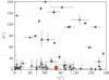 |
Fig. 3 Projected orbit-orbit angle (γ) against the projected obliquity (λ) based on the table by Rice et al. (2024). Markers are coloured according to the effective temperature of the host star with blue (red) denoting stars cooler (hotter) than 6105 K, as found to be appropriate for binary systems by Wang et al. (2026). The triangles demarcate triple star systems, and TOI-13 3 3 is indicated with a square. As in Rice et al. (2024) systems with either σλ> 25° or σγ > 25° are shown with low opacity. |
5 Conclusions
Using data from the FIES spectrograph we have measured a projected obliquity of λ = -5 ± 10° for the hot Jupiter TOI-1333Ab, demonstrating that the planetary orbit is well aligned with the stellar spin axis of its host star. Such low obliquity is naturally consistent with disc-driven migration, which is typically expected to preserve alignment and produce low eccentricities, in agreement with the modest eccentricity reported by R21. However, the wide stellar companion TOI-1333B also makes high-e migration via ZKL oscillations a viable alternative, with subsequent tidal dissipation acting to shrink, circularise, and potentially realign the system. Given the planet’s close-in orbit and high planet-to-star mass ratio, tidal interactions could have been efficient, even though TOI-1333A lies above the canonical Kraft break, where hot Jupiter hosts are more frequently found to be misaligned.
In the context of recent studies that suggest a lower effective temperature threshold for misalignment in binary systems (Wang et al. 2026), TOI-1333A is part of a group of well-aligned exceptions. This could indicate that tidal realignment may remain effective under a broader range of stellar and dynamical conditions than commonly assumed.
Placed in the wider λ, γ landscape of planets in binary systems, TOI-1333 occupies a relatively isolated region with an orbit-orbit angle of γ =81.5 ± 1.1°. This combination of low projected obliquity and a near face-on configuration underscores the complex role of stellar companions in both exciting and damping misalignments. TOI-1333 therefore provides a valuable system for testing competing migration pathways and tidal realignment scenarios in hot-Jupiter systems with wide stellar companions.
Acknowledgements
We are grateful to the anonymous referee for providing insightful comments that helped improve the quality of the manuscript. This work was supported by a research grant (42101) from VILLUM FONDEN and from the Danish Council for Independent Research through grant No.2032-00230B. M.S.L. is supported by the Independent Research Fund Denmark’s Inge Lehmann program (grant agreement No. 1131-00014B). Based on observations made with the Nordic Optical Telescope, owned in collaboration by the University of Turku and Aarhus University, and operated jointly by Aarhus University, the University of Turku, and the University of Oslo, representing Denmark, Finland and Norway, the University of Iceland and Stockholm University at the Observatorio del Roque de los Muchachos, La Palma, Spain, of the Instituto de Astrofisica de Canarias. The NOT data were obtained under program ID P71007. This work presents results from the European Space Agency (ESA) space mission Gaia. Gaia data are being processed by the Gaia Data Processing and Analysis Consortium (DPAC). Funding for the DPAC is provided by national institutions, in particular the institutions participating in the Gaia MultiLateral Agreement (MLA). The Gaia mission website is https://www.cosmos.esa.int/gaia. The Gaia archive website is https://archives.esac.esa.int/gaia. This work made use of the following Python packages; NumPy (Harris et al. 2020), SciPy (Virtanen et al. 2020), Matplotlib (Hunter 2007), astroquery (Ginsburg et al. 2019), corner (Foreman-Mackey 2016), and Astropy (Astropy Collaboration 2013; Astropy Collaboration 2018, 2022).
References
- Albrecht, S., Winn, J. N., Johnson, J. A., et al. 2012, ApJ, 757, 18 [NASA ADS] [CrossRef] [Google Scholar]
- Albrecht, S. H., Dawson, R. I., & Winn, J. N. 2022, PASP, 134, 082001 [NASA ADS] [CrossRef] [Google Scholar]
- Astropy Collaboration (Robitaille, T. P., et al.) 2013, A&A, 558, A33 [NASA ADS] [CrossRef] [EDP Sciences] [Google Scholar]
- Astropy Collaboration (Price-Whelan, A. M., et al.) 2018, AJ, 156, 123 [Google Scholar]
- Astropy Collaboration (Price-Whelan, A. M., et al.) 2022, ApJ, 935, 167 [NASA ADS] [CrossRef] [Google Scholar]
- Behmard, A., Dai, F., & Howard, A. W. 2022, AJ, 163, 160 [NASA ADS] [CrossRef] [Google Scholar]
- Beyer, A. C., & White, R. J. 2024, ApJ, 973, 28 [Google Scholar]
- Biddle, L. I., Bowler, B. P., Morgan, M., Tran, Q. H., & Wu, Y.-L. 2025, Nature, 644, 356 [Google Scholar]
- Bruntt, H., Bedding, T. R., Quirion, P.-O., et al. 2010, MNRAS, 405, 1907 [NASA ADS] [Google Scholar]
- Buchhave, L. A., Latham, D. W., Johansen, A., et al. 2012, Nature, 486, 375 [NASA ADS] [Google Scholar]
- Claret, A. 2018, A&A, 618, A20 [NASA ADS] [CrossRef] [EDP Sciences] [Google Scholar]
- Claret, A., Hauschildt, P. H., & Witte, S. 2013, A&A, 552, A16 [NASA ADS] [CrossRef] [EDP Sciences] [Google Scholar]
- Djupvik, A. A., & Andersen, J. 2010, in Astrophysics and Space Science Proceedings, 14, Highlights of Spanish Astrophysics V, eds. J. M. Diego, L. J. Goicoechea, J. I. González-Serrano, & J. Gorgas, 211 [Google Scholar]
- Doyle, A. P., Davies, G. R., Smalley, B., Chaplin, W. J., & Elsworth, Y. 2014, MNRAS, 444, 3592 [Google Scholar]
- Espinoza-Retamal, J. I., Jordán, A., Brahm, R., et al. 2025, AJ, 170, 70 [Google Scholar]
- Fabrycky, D., & Tremaine, S. 2007, ApJ, 669, 1298 [NASA ADS] [CrossRef] [Google Scholar]
- Fabrycky, D. C., & Winn, J. N. 2009, ApJ, 696, 1230 [NASA ADS] [CrossRef] [Google Scholar]
- Foreman-Mackey, D. 2016, J. Open Source Softw., 1, 24 [Google Scholar]
- Foreman-Mackey, D., Hogg, D. W., Lang, D., & Goodman, J. 2013, PASP, 125, 306 [Google Scholar]
- Foreman-Mackey, D., Agol, E., Angus, R., & Ambikasaran, S. 2017, AJ, 154, 220 [NASA ADS] [CrossRef] [Google Scholar]
- Fûrész, G. 2008, PhD thesis, University of Szeged, Hungary [Google Scholar]
- Gaia Collaboration (Prusti, T., et al.) 2016, A&A, 595, A1 [NASA ADS] [CrossRef] [EDP Sciences] [Google Scholar]
- Gaia Collaboration (Brown, A. G. A., et al.) 2018, A&A, 616, A1 [NASA ADS] [CrossRef] [EDP Sciences] [Google Scholar]
- Gaia Collaboration (Vallenari, A., et al.) 2023, A&A, 674, A1 [NASA ADS] [CrossRef] [EDP Sciences] [Google Scholar]
- Giacalone, S., Howard, A. W., Rubenzahl, R. A., et al. 2025, PASP, 137, 074401 [Google Scholar]
- Ginsburg, A., SipOcz, B. M., Brasseur, C. E., et al. 2019, AJ, 157, 98 [NASA ADS] [CrossRef] [Google Scholar]
- Gupta, A. F., Millholland, S. C., Im, H., et al. 2024, Nature, 632, 50 [NASA ADS] [CrossRef] [Google Scholar]
- Han, T., Robertson, P., Brandt, T. D., et al. 2025, ApJ, 988, L4 [Google Scholar]
- Harris, C. R., Millman, K. J., van der Walt, S. J., et al. 2020, Nature, 585, 357 [NASA ADS] [CrossRef] [Google Scholar]
- Hébrard, G., Désert, J.-M., Díaz, R. F., et al. 2010, A&A, 516, A95 [CrossRef] [EDP Sciences] [Google Scholar]
- Hirano, T., Suto, Y., Winn, J. N., et al. 2011, ApJ, 742, 69 [NASA ADS] [CrossRef] [Google Scholar]
- Hjorth, M., Albrecht, S., Hirano, T., et al. 2021, PNAS, 118, e2017418118 [NASA ADS] [CrossRef] [Google Scholar]
- Høg, E., Fabricius, C., Makarov, V. V., et al. 2000, A&A, 355, L27 [Google Scholar]
- Hunter, J. D. 2007, Comput. Sci. Eng., 9, 90 [NASA ADS] [CrossRef] [Google Scholar]
- Kálmán, S., Csizmadia, S., Pál, A., & Szabó, G. M. 2025, RNAAS, 9, 33 [Google Scholar]
- Knudstrup, E., & Albrecht, S. H. 2022, A&A, 660, A99 [NASA ADS] [CrossRef] [EDP Sciences] [Google Scholar]
- Knudstrup, E., Albrecht, S. H., Winn, J. N., et al. 2024, A&A, 690, A379 [NASA ADS] [CrossRef] [EDP Sciences] [Google Scholar]
- Kozai, Y. 1962, AJ, 67, 591 [Google Scholar]
- Kreidberg, L. 2015, PASP, 127, 1161 [Google Scholar]
- Lidov, M. L. 1962, Planet. Space Sci., 9, 719 [Google Scholar]
- Lightkurve Collaboration (Cardoso, J. V. d. M., et al.) 2018, Lightkurve: Kepler and TESS time series analysis in Python, Astrophysics Source Code Library [Google Scholar]
- Lin, D. N. C., Bodenheimer, P., & Richardson, D. C. 1996, Nature, 380, 606 [Google Scholar]
- Mandel, K., & Agol, E. 2002, ApJ, 580, L171 [Google Scholar]
- Masuda, K., & Winn, J. N. 2020, AJ, 159, 81 [NASA ADS] [CrossRef] [Google Scholar]
- McLaughlin, D. B. 1924, ApJ, 60, 22 [Google Scholar]
- Michel, K.-U., & Mugrauer, M. 2024, MNRAS, 527, 3183 [Google Scholar]
- Naef, D., Latham, D. W., Mayor, M., et al. 2001, A&A, 375, L27 [NASA ADS] [CrossRef] [EDP Sciences] [Google Scholar]
- Pepper, J., Pogge, R. W., DePoy, D. L., et al. 2007, PASP, 119, 923 [NASA ADS] [CrossRef] [Google Scholar]
- Polanski, A. S., Crossfield, I. J. M., Seifahrt, A., et al. 2025, AJ, 170, 182 [Google Scholar]
- Rasmussen, C. E., & Williams, C. K. I. 2006, Gaussian Processes for Machine Learning [Google Scholar]
- Rice, M., Gerbig, K., & Vanderburg, A. 2024, AJ, 167, 126 [NASA ADS] [CrossRef] [Google Scholar]
- Ricker, G. R., Winn, J. N., Vanderspek, R., et al. 2015, J. Astron. Telesc. Instrum. Syst., 1, 014003 [Google Scholar]
- Rodriguez, J. E., Quinn, S. N., Zhou, G., et al. 2021, AJ, 161, 194 [NASA ADS] [CrossRef] [Google Scholar]
- Rossiter, R. A. 1924, ApJ, 60, 15 [Google Scholar]
- Socrates, A., Katz, B., Dong, S., & Tremaine, S. 2012, ApJ, 750, 106 [Google Scholar]
- Telting, J. H., Avila, G., Buchhave, L., et al. 2014, Astron. Nachr., 335, 41 [Google Scholar]
- Veldhuis, H., Espinoza-Retamal, J. I., Stefansson, G., et al. 2026, A&A, in press, https://doi.org/10.1051/0004-6361/202556348 [Google Scholar]
- Virtanen, P., Gommers, R., Oliphant, T. E., et al. 2020, Nat. Methods, 17, 261 [Google Scholar]
- von Zeipel, H. 1910, Astron. Nachr., 183, 345 [Google Scholar]
- Wang, X.-Y., Wang, S., & Ong, J. M. J. 2026, ApJ, 996, L7 [Google Scholar]
- Weisserman, D., Gillis, E., Cloutier, R., et al. 2025, AJ, 170, 313 [Google Scholar]
- Winn, J. N., Fabrycky, D., Albrecht, S., & Johnson, J. A. 2010, ApJ, 718, L145 [Google Scholar]
- Wu, Y., & Murray, N. 2003, ApJ, 589, 605 [Google Scholar]
- Yee, S. W., Stefánsson, G., Thorngren, D., et al. 2025, AJ, 169, 225 [Google Scholar]
- Zak, J., Bocchieri, A., Sedaghati, E., et al. 2024, A&A, 686, A147 [NASA ADS] [CrossRef] [EDP Sciences] [Google Scholar]
- Zak, J., Boffin, H. M. J., Bocchieri, A., et al. 2025a, AJ, 170, 274 [Google Scholar]
- Zak, J., Boffin, H. M. J., Sedaghati, E., et al. 2025b, A&A, 694, A91 [NASA ADS] [CrossRef] [EDP Sciences] [Google Scholar]
- Zechmeister, M., Reiners, A., Amado, P. J., et al. 2018, A&A, 609, A12 [NASA ADS] [CrossRef] [EDP Sciences] [Google Scholar]
Appendix A Stellar inclination and obliquity
The light curve from TOI-1333A clearly shows rotational modulation (Figure B.2). R21 reported a stellar rotation period of Prot = 5.300 ± 0.159 d based on both the TESS data from Sector 15 and 16 as well as photometry from the Kilodegree Extremely Little Telescope (KELT; Pepper et al. 2007) survey. As R21, we note that the rotational modulation seen in the TESS and KELT light curves might be attributed to blended sources instead as both have rather large pixel scales (21″ and 23″, respectively).
Should the modulation be coming from a blended source, it is most likely a rather bright star in the aperture mask. The two brightest stars within the mask are the bound companion, TOI-1333B, with G = 12.66 (Gaia Collaboration 2023, ΔG = 3.30 wrt. TOI-1333A) and TYC 3595-1186-2 with V = 10.15 and G = 9.98 (ΔG = 0.62 wrt. TOI-1333A). TOI-1333B is a K-dwarf (M* = 0.843 M⊙, Teff = 4995 K; Michel & Mugrauer 2024) and therefore seems unlikely to be the source of the modulation given the rather rapid rotation. It seems more probable that TYC 35951186-2 could be the source; information on the star is sparse, but Gaia DR2 (Gaia Collaboration 2018) gives an effective temperature of 6480 K and this star therefore seems to be slightly hotter than TOI-1333A. This is supported by the colour index with B - V = 0.32 for this star compared to B - V = 0.42 for TOI-1333A.
What might also suggest that TYC 3595-1186-2 is the source is that despite the similarity in brightness, the error on the mean flux in the Gaia G-band is around 0.016% for TOI-1333A and 0.033% for TYC 3595-1186-2, which could hint at an additional source of photometric variability for TYC 3595-1186-2. Spectroscopic follow-up observations of TYC 3595-1186-2 and of course future resolved photometric time series of both TYC 3595-1186-2 and TOI-1333A could help shed light on the source of the modulation.
Even though we do not believe TOI-1333A to be the source of the rotational modulation, we nonetheless investigated what the stellar inclination and 3D obliquity would be assuming TOI-1333A is the source. Following the approach in Hjorth et al. (2021) we determined the rotation period using all four TESS sectors and obtained a value of 5.17 ± 0.05 d, consistent with the value from R21. As we have now determined Prot, we can use this with v sin i* = 14.2 ± 0.5 km s−1 and R⋆ =  R⊙ (R21) to derive the stellar inclination. We did this using the formulation in Masuda & Winn (2020) to account for the fact that v sin i* and v are not statistically independent. From this we found cos i* =
  and i* =
  .
.
The (3D) obliquity can then be determined from
 (A.1)
(A.1)
where io is the orbital inclination. We used our posteriors from Section 3 to create the corresponding distributions for ψ resulting in 40 ± 4°.
For context, if ψ were 30° the chance of observing λ a factor of two smaller than that is around 35% (with lower probabilities for larger values of ψ Fabrycky & Winn 2009). This also does not favour the value derived for ψ above. While the arguments presented above are not conclusive, we believe the conservative approach is to not claim a measurement for ψ.
Appendix B Additional figures and tables
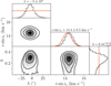 |
Fig. B.1 Posterior distributions from our MCMC showing the correlation between λ, v sin i*, and b. The red curves in the histogram denote the priors applied. |
FIES RVs of TOI-1333 on the night of 12-08-2025.
Posterior values for all fitting parameters in our MCMC.
Extension to the table by Rice et al. (2024).
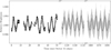 |
Fig. B.2 TESS light curves of TOI-1333 showing the rotational modulation, which cannot necessarily be attributed to TOI-1333A. The colourcoding is the same as in Figure 1. The GP model used for detrending is shown as the white line with a black outline. Transits were removed by subtracting the best-fitting transit model. |
As of 12-01-2026.
Although we note they also required the binary inclination to be edgeon, which we do not calculate here.
All Tables
All Figures
|
Fig. 1 TESS light curve of TOI-1333 folded on the transit of TOI-1333Ab. The black dots demarcate observations taken with a cadence of 30 min. The grey points indicate the 2 min. cadence data. The bestfitting transit model is shown as the solid white line, and the residuals (in parts per thousand) are shown in the bottom. |
| In the text | |
|
Fig. 2 FIES RVs of TOI-1333A after subtracting the best-fitting Keplerian. The solid line denotes the best-fitting model for the RM effect, and the shaded areas represent the 1- and 2-σ confidence intervals. |
| In the text | |
|
Fig. 3 Projected orbit-orbit angle (γ) against the projected obliquity (λ) based on the table by Rice et al. (2024). Markers are coloured according to the effective temperature of the host star with blue (red) denoting stars cooler (hotter) than 6105 K, as found to be appropriate for binary systems by Wang et al. (2026). The triangles demarcate triple star systems, and TOI-13 3 3 is indicated with a square. As in Rice et al. (2024) systems with either σλ> 25° or σγ > 25° are shown with low opacity. |
| In the text | |
|
Fig. B.1 Posterior distributions from our MCMC showing the correlation between λ, v sin i*, and b. The red curves in the histogram denote the priors applied. |
| In the text | |
|
Fig. B.2 TESS light curves of TOI-1333 showing the rotational modulation, which cannot necessarily be attributed to TOI-1333A. The colourcoding is the same as in Figure 1. The GP model used for detrending is shown as the white line with a black outline. Transits were removed by subtracting the best-fitting transit model. |
| In the text | |
Current usage metrics show cumulative count of Article Views (full-text article views including HTML views, PDF and ePub downloads, according to the available data) and Abstracts Views on Vision4Press platform.
Data correspond to usage on the plateform after 2015. The current usage metrics is available 48-96 hours after online publication and is updated daily on week days.
Initial download of the metrics may take a while.