| Issue |
A&A
Volume 708, April 2026
|
|
|---|---|---|
| Article Number | L14 | |
| Number of page(s) | 9 | |
| Section | Letters to the Editor | |
| DOI | https://doi.org/10.1051/0004-6361/202659069 | |
| Published online | 14 April 2026 | |
Letter to the Editor
Magneto-archeology of white dwarfs
Revisiting the fossil field scenario with observational constraints during the red giant branch
1
Institute of Science and Technology Austria (ISTA), Am Campus 1, Klosterneuburg, Austria
2
Grupo de Evolución Estelar y Pulsaciones, Facultad de Ciencias Astronómicas y Geofísicas, Universidad Nacional de La Plata, Paseo del Bosque s/n (1900), La Plata, Argentina
3
Instituto de Astrofísica La Plata, CONICET-UNLP, Paseo del Bosque s/n, (1900) La Plata, Argentina
4
Center for Astrophysics | Harvard & Smithsonian, 60 Garden Street, Cambridge, MA 02138, USA
⋆ Corresponding author: This email address is being protected from spambots. You need JavaScript enabled to view it.
Received:
21
January
2026
Accepted:
16
March
2026
Abstract
The detection of strong, large-scale magnetic fields at the surfaces of the oldest white dwarfs might point toward a hidden internal magnetic field slowly rising to the surface. In addition, strong magnetic fields have recently been measured through asteroseismology in the radiative interiors of red giant stars, the progenitors of white dwarfs. To investigate the potential connection between these observations, we revisited the fossil field framework using asteroseismic detections to constrain the strength of such magnetic fields as red giants evolve into the white dwarf stage. We assumed that the magnetic field was either created during the core convection on the main sequence or that it fills the radiative interior as the star evolves on the red giant branch. From these initial conditions, we evolved the magnetic flux, allowing for magnetic diffusion along the evolution of a modeled 1.5 M⊙ star. We find that measured field strengths in red giants attributed to the hydrogen-burning shell are compatible with the field amplitudes and emergence timescales of magnetized white dwarfs. On the contrary, magnetic fields generated solely from a convective-core dynamo on the main sequence and detectable on the red giant branch would be buried too deep in the star and would not match the breakout timescales or the field strengths of magnetic white dwarfs. Therefore, for us to connect magnetic fields observed along the late evolution of stars via a fossil field we would need to find a broadly magnetized internal radiative zone on the red giant branch.
Key words: stars: evolution / stars: interiors / stars: low-mass / stars: magnetic field / stars: oscillations / white dwarfs
© The Authors 2026
 Open Access article, published by EDP Sciences, under the terms of the Creative Commons Attribution License (https://creativecommons.org/licenses/by/4.0), which permits unrestricted use, distribution, and reproduction in any medium, provided the original work is properly cited.
This article is published in open access under the Subscribe to Open model. This email address is being protected from spambots. You need JavaScript enabled to view it. to support open access publication.
1. Introduction
White dwarfs (WDs) give us key insights into the properties of the cores of their progenitors. In particular, exposed stable magnetic fields at the surface of WDs might be related to past core magnetism (e.g., Quentin & Tout 2018; Ferrario et al. 2020), which plays a crucial role in determining the internal distribution of angular momentum as stars evolve (e.g., Takahashi & Langer 2021).
Bagnulo & Landstreet (2022) and Moss et al. (2025) measured the surface magnetic fields of close-by WDs. They find an incidence of surface magnetism of roughly 6% for WDs with field strengths of ∼1 − 100 MG. This increases to 20% if weakly magnetized WDs (< 1 MG) are also considered (Bagnulo & Landstreet 2022). In addition, the incidence of magnetism increases with age for typical WDs resulting from single-star evolution in the mass range 0.5–1 M⊙. Two key questions are therefore where these stable surface magnetic fields originate, and why their emergence seems to be delayed along the cooling sequence. If we rule out binary interaction channels, magnetic fields at the surface of WDs are likely created either by a crystallization dynamo (e.g., Isern et al. 2017; Ginzburg et al. 2022; Fuentes et al. 2024; Castro-Tapia et al. 2024a) or via the fossil field scenario (FFS), which was studied recently by, for instance, Camisassa et al. (2024, hereafter C24) and Castro-Tapia et al. (2026, hereafter CT26). Using typical dynamo efficiencies in the convective core during the main sequence (MS) and conserving the magnetic flux all the way to the WD phase, C24 and CT26 demonstrate that the FFS leads to an emergence of magnetism at the surface of WDs on timescales compatible with observations. However, one key additional observational constraint absent from the picture is the recent detection of magnetic fields in the interior of WD progenitors, red giants (RGs). Magnetic fields have been detected in the radiative interiors of RGs: a few dozen magnetic RG cores have been confirmed to date (see Hatt et al. 2024, and references within). We revisited the FFS, including these new asteroseismic constraints from early stages, and investigated when and with what properties resulting fossil fields could explain the emergence of magnetism at the surface of old WDs.
2. Magnetic evolution framework
2.1. Magnetic evolution scenarios and configurations
We considered three different origins and initial setups for the evolution of the magnetic field. First, we assumed that the field comes from the convective core during the MS stage and starts evolving at the end of the MS (Scenario A, Fig. 1, dark blue). Scenario B assumes the same but also allows for the magnetic extent to vary and for the magnetic field to diffuse into the radiative envelope during the MS stage, resulting in a larger magnetic region at the end of the MS (Scenario B, Fig. 1, light blue). Lastly, we placed a stable field directly in the full radiative interior during the red giant branch (RGB) stage (Scenario C, Fig. 1, red). Possible formation channels for such a field and additional details on all three scenarios are given in Appendix A. The initial internal fields’ extent is limited to the radiative zone, and we neglected the impact of convection and convective dynamo action on the diffusion of the large-scale internal magnetic field during RG stages due to the expected slow motion and low efficiency of the dynamo action (Aurière et al. 2015; Amard et al. 2024) and the unconstrained coupling with the stable field. We considered dipolar magnetic fields extracted from the most stable initial field configurations, following the works of Broderick & Narayan (2007), Braithwaite (2008), and Duez & Mathis (2010). Additional information on the magnetic field profiles can be found in Appendix B.
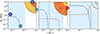 |
Fig. 1. Considered magnetic field configurations at different evolutionary stages of a typical 1.5 M⊙ star. The central field strengths are set such that asteroseismic detections of all three fields would measure 100 kG during the RGB stage (see Appendix C). Left panel: Scenarios A (dark blue line) and B (light blue line) are created by the convective core during the MS stage and start evolving as a large-scale stable field at the end of the MS. Middle panel: Magnetic fields during the RGB stage when the typical oscillation frequency of the star reaches 150 μHz. The two fields for Scenarios A and B are now buried below the hydrogen-burning shell (dashed line). Scenario C (red line) starts its evolution here and fills the entire radiative interior. Right panel: Magnetic field configurations for all three scenarios at the start of the WD cooling sequence. The blue-shaded region corresponds to the radial extent of the WD mass at different evolutionary stages. |
2.2. Observational constraints from asteroseismology
To calibrate the strength of the fields we considered, we used constraints from the largest sample of magnetic measurements in the radiative interior of RGs, that of Hatt et al. (2024). We evolved a representative model from their sample with a mass of 1.5 M⊙ (Z = 0.02) using Modules for Experiments in Stellar Astrophysics (MESA1; Jermyn et al. 2023, and references therein) from the MS to the WD cooling sequence to provide the background stellar structure for the magnetic field evolution calculation. To constrain the magnetic field, we chose the RG model whose typical oscillation mode frequency was closest to 150 μHz. At this evolutionary stage, we normalized our field configurations to match the signatures measured in Hatt et al. (2024). To do so, we used the code magsplitpy and followed the method outlined in Appendix C, which is based on the RG literature (Das et al. 2020; Bugnet et al. 2021; Mathis et al. 2021; Li et al. 2022; Mathis & Bugnet 2023; Bhattacharya et al. 2024; Das et al. 2024). Our normalization thus resulted in core-averaged squared radial field strengths, ⟨Br2⟩, that would be typically measured from observing oscillation modes for the chosen RG model (see Appendix C). We illustrate  kG in Fig. 1. Typical detected field strengths range from ∼10 kG up to ∼200 kG (Hatt et al. 2024), with the highest detection being above ∼600 kG (Deheuvels et al. 2023).
2.3. Numerical methods for determining the evolution of magnetic fields during stellar evolution
We evolved magnetic fields via flux conservation and diffusion. Most work on WDs regarding this relied on calculating ohmic diffusion timescales and did not consider the configuration of the magnetic field itself (e.g., Cumming 2002, C24). However, more recent work has relied on the evolving magnetic fields on the WD cooling sequence from initial step function-like field configurations (Castro-Tapia et al. 2024b; Blatman et al. 2025, CT26). This approximation works well during the WD cooling phase, when the structural evolution of the star can be neglected. However, during earlier evolutionary stages, nuclear burning creates structural changes in the stellar interior, which can drastically change the size and radial distribution of the magnetized mass. Especially strong density gradients, such as around the hydrogen-burning shell (H-shell), can have a strong effect on the magnetic flux distribution. Thus, for earlier evolutionary stages, we needed to take the changes in the stellar structure into account and instead solve the full induction equation:
 (1)
(1)
with B the magnetic field, u the fluid velocity, and η the magnetic diffusivity. To solve it along the evolution, we followed the method described in Takahashi & Langer (2021, Sect. 2.2). Using MESA, we calculated all relevant structure parameters. In particular, for the magnetic diffusivity, we followed the prescriptions of Potekhin et al. (1999) and Stygar et al. (2002) for the degenerate and non-degenerate regions, respectively, and linearly interpolated between the two formulations in the intermediate region. We neglected the small effect the crystallization of the WD core has on the magnetic diffusivity. For more details, see Appendix D.
3. Results and discussions
3.1. Magnetic evolution before the white dwarf stage
Figure 1 shows how fields from the different scenarios evolve alongside stellar evolution. We show that magnetic fields confined within the MS convective core (resulting from Scenarios A and B) are buried deep below the H-shell on the RGB. The sensitivity of the modes to the magnetic field is dominant at this H-shell (see Appendix C). Therefore, to be detected as a core-averaged 100 kG field via asteroseismology on the RGB, it has to reach a huge central strength on the order of ∼10 MG, which is about half of the critical field above which the mode core energy would be suppressed (Fuller et al. 2015).
However, Scenario C depicts a different picture, as the magnetic field extends beyond the H-shell. An interesting feature can be seen in the initial WD field for this scenario. Rather than being centered at the core, this field configuration peaks in a shell instead. This shell configuration comes from the steep density gradient around the H-shell during the RGB, which compresses the magnetic field as it slowly moves outward. This only happens to the magnetic field of Scenario C because the other two fields vanish before reaching the H-shell (details on this effect are given in Appendix E).
3.2. Emergence of the fossil magnetic fields at the surface
In Fig. 2 we summarize our results, calibrating when our various FFSs result in the emergence of magnetic fields at the surface of WDs (see also Appendix F). We show that most detected magnetic WDs from Bagnulo & Landstreet (2022) and Moss et al. (2025) can be explained by Scenario C with the core-averaged RGB field strengths determined by Hatt et al. (2024), which range from 10 kG to 200 kG (red-shaded region). While there are also a few magnetic WDs outside this region, most of them can be explained by the higher RGB field strengths determined by Deheuvels et al. (2023), which can reach at least 600 kG (dashed black line). Thus, almost all magnetic WDs in the mass range (0.5–0.64 M⊙) compatible with the mass distribution of detected magnetic RGs can be explained by a magnetic field that has a significant amplitude far above the H-shell during the RGB stage (Scenario C; see Appendix G.1 for more details).
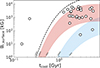 |
Fig. 2. Radial surface field strength as a function of the cooling age of the WD for Scenarios B (blue) and C (red). The shaded regions show the evolution for varying field strengths on the RGB between 10 kG (bottom) and 200 kG (top), the range detected in Hatt et al. (2024). The dashed line shows the emergence of the strongest detected RGB field of 600 kG (Deheuvels et al. 2023) and places a lower limit on the FFS emergence timescale. The white circles show detected magnetic WDs from the Bagnulo & Landstreet (2022) and Moss et al. (2025) samples in the mass range [0.5 − 0.64] M⊙. |
In contrast, the magnetic field of Scenario B can only explain a very few old, weakly magnetized WDs. Even if we normalize the field to 600 kG during the RGB stage, this can explain at most a third of the magnetic WDs shown in Fig. 2. For ease of reading, we chose not to show Scenario A in Fig. 2 as its field strength is even lower than that of Scenario B. Two very young magnetic WDs can very clearly not be reproduced with any of our magnetic field configurations and are thus incompatible with our formalism.
To demonstrate the robustness of these conclusions, we discuss their dependence on stellar mass and on the extent of the magnetic field during the RGB stage in Appendix G.
3.3. Conclusions on the fossil field scenario
From Fig. 2, we conclude that fossil fields resulting from internal RG fields near the H-shell emerge at the surface of WDs on a timescale compatible with spectroscopic observations. We therefore confirm the results of C24 and CT26, that the FFS is a great candidate to explain WD magnetic field amplitudes and emergence timescales.
However, our study points out that, to link the magnetic fields detected in RG cores to the WD stage, magnetic fields cannot result solely from a convective-core dynamo during the MS stage. This conclusion differs from that of C24 and CT26 due to the stable initial radial profile of the field we considered, following Braithwaite (2008), Broderick & Narayan (2007), and Duez & Mathis (2010), as opposed to the constant radial magnetic energy assumed in C24 and CT26. Such an extended strong field at the end of the MS is not realistic if we consider only the stabilization of the core dynamo effect, during which the reconnection of the field results in a loss of magnetic energy, with a flattened radial energy distribution decaying much faster compared to more tapered distributions (this work). Thus, even though the core dynamo on the MS can create fields on the order of ∼1 − 100 kG, constant radial field distributions are likely to stabilize into much weaker fields compared to the more realistic profiles that are present once the convection ends. In addition, the resulting stable large-scale poloidal component of the field (Braithwaite 2008) is likely confined in the previously magnetized region (Broderick & Narayan 2007; Duez & Mathis 2010).
We also emphasize the recent inference of a nearly pure toroidal field at the outer boundary of the convective core during the MS (Takata et al. 2026), which reinforces the conclusion that, if rotational effects are not at play, the radial component of the magnetic field remains contained in the convective core (which is also in agreement with massive star convective core simulations; e.g., Ratnasingam et al. 2024). The strong uniform field used in CT26 is in fact more representative of an extended magnetized radiative zone similar to our Scenario C, which could result (i) from the convective-core dynamo coupled with a fossil field in the MS radiative zone (Hidalgo et al. 2025), (ii) from the coupled effects of core dynamo and fast rotation during the MS (enhancing the advection of the core dynamo in the outer layers; Hidalgo et al. 2024), or (iii) directly from a dynamo action in an RG’s radiative interior (and therefore unlinked to the MS core dynamo; e.g., Fuller et al. 2019).
Scenario C leads to a radial magnetic field profile confined in a shell at a radius of approximately 35% of the stellar radius at the start of the WD cooling sequence. This structural effect is due to the local magnetic flux conservation in its mass coordinate, which compresses the field around the H-shell during the RGB (see Appendix E for details on the origin of the confinement). The long-term stability of such a geometry, which differs from the Prendergast-like stable profiles discussed in Kaufman et al. (2022), remains to be studied (this radial magnetic profile is, however, robust against magnetic diffusion on gigayear timescales; see Appendix F). A second possible extension of our work is to include the impact of the formation of the small convective core during the core-helium-burning phase, as it is expected to generate additional magnetic energy in the core, potentially strengthening the deep radial magnetic profile even further (see a similar configuration on the MS in Featherstone et al. 2009). Both analyses require dedicated 3D simulations and are beyond the scope of our study.
Under the FFS, stars sustain their magnetic fields all throughout their evolution. Distinguishing between the FFS and the crystallization scenario, for example, from Isern et al. (2017) or contemporary fields in radiative zones, as in Fuller et al. (2019), is crucial for a better constraint on angular momentum and chemical transport in stars. The new area of magneto-asteroseismology focused on the RGB, MS, and even young WDs (e.g., Rui et al. 2025) is key to further investigating the possibility of magnetic survival across stellar ages.
Data availability
We used MESA version 24.08.1. All inlists and relevant files are available on Zenodo at https://doi.org/10.5281/zenodo.19232789
Acknowledgments
The authors thank the referee for their helpful and constructive report, which has significantly enhanced the quality of the manuscript. The authors thank I. Caiazzo, L. Ferrario, and L. Buchele for very useful discussions. L. Barrault, L. Bugnet, and L. Einramhof gratefully acknowledge support from the European Research Council (ERC) under the Horizon Europe programme (Calcifer; Starting Grant agreement N°101165631). L. Barrault acknowledges the support of the Austrian Academy of Sciences through the Doctoral Fellowship Programme (DOC) of the Austrian Academy of Sciences 27648. While partially funded by the European Union, views and opinions expressed are, however, those of the authors only and do not necessarily reflect those of the European Union or the European Research Council. Neither the European Union nor the granting authority can be held responsible for them.
References
- Amard, L., Brun, A. S., & Palacios, A. 2024, ApJ, 974, 311 [Google Scholar]
- Aurière, M., Konstantinova-Antova, R., Charbonnel, C., et al. 2015, A&A, 574, A90 [Google Scholar]
- Bagnulo, S., & Landstreet, J. D. 2022, ApJ, 935, L12 [NASA ADS] [CrossRef] [Google Scholar]
- Barrera, R. G., Estevez, G. A., & Giraldo, J. 1985, Eur. J. Phys., 6, 287 [Google Scholar]
- Bhattacharya, S., Das, S. B., Bugnet, L., Panda, S., & Hanasoge, S. M. 2024, ApJ, 970, 42 [NASA ADS] [CrossRef] [Google Scholar]
- Blatman, D., Rui, N. Z., Ginzburg, S., & Fuller, J. 2025, MNRAS, 542, 2345 [Google Scholar]
- Braithwaite, J. 2008, MNRAS, 386, 1947 [Google Scholar]
- Broderick, A. E., & Narayan, R. 2007, MNRAS, 383, 943 [CrossRef] [Google Scholar]
- Bugnet, L., Prat, V., Mathis, S., et al. 2021, A&A, 650, A53 [NASA ADS] [CrossRef] [EDP Sciences] [Google Scholar]
- Camisassa, M., Fuentes, J. R., Schreiber, M. R., et al. 2024, A&A, 691, L21 [NASA ADS] [CrossRef] [EDP Sciences] [Google Scholar]
- Castro-Tapia, M., Cumming, A., & Fuentes, J. R. 2024a, ApJ, 969, 10 [NASA ADS] [CrossRef] [Google Scholar]
- Castro-Tapia, M., Zhang, S., & Cumming, A. 2024b, ApJ, 975, 63 [NASA ADS] [CrossRef] [Google Scholar]
- Castro-Tapia, M., Camisassa, M., & Zhang, S. 2026, ApJ, 998, 28 [Google Scholar]
- Cumming, A. 2002, MNRAS, 333, 589 [NASA ADS] [CrossRef] [Google Scholar]
- Das, S. B., Chakraborty, T., Hanasoge, S. M., & Tromp, J. 2020, ApJ, 897, 38 [NASA ADS] [CrossRef] [Google Scholar]
- Das, S. B., Einramhof, L., & Bugnet, L. 2024, A&A, 690, A217 [NASA ADS] [CrossRef] [EDP Sciences] [Google Scholar]
- Deheuvels, S., Li, G., Ballot, J., & Lignières, F. 2023, A&A, 670, L16 [NASA ADS] [CrossRef] [EDP Sciences] [Google Scholar]
- Duez, V., & Mathis, S. 2010, A&A, 517, A58 [NASA ADS] [CrossRef] [EDP Sciences] [Google Scholar]
- Featherstone, N. A., Browning, M. K., Brun, A. S., & Toomre, J. 2009, ApJ, 705, 1000 [Google Scholar]
- Ferrario, L., Wickramasinghe, D., & Kawka, A. 2020, Adv. Space Res., 66, 1025 [NASA ADS] [CrossRef] [Google Scholar]
- Fuentes, J. R., Castro-Tapia, M., & Cumming, A. 2024, ApJ, 964, L15 [NASA ADS] [CrossRef] [Google Scholar]
- Fuller, J., Cantiello, M., Stello, D., Garcia, R. A., & Bildsten, L. 2015, Science, 350, 423 [Google Scholar]
- Fuller, J., Piro, A. L., & Jermyn, A. S. 2019, MNRAS, 485, 3661 [NASA ADS] [Google Scholar]
- Ginzburg, S., Fuller, J., Kawka, A., & Caiazzo, I. 2022, MNRAS, 514, 4111 [NASA ADS] [CrossRef] [Google Scholar]
- Hardy, F., Dufour, P., & Jordan, S. 2023, MNRAS, 520, 6111 [CrossRef] [Google Scholar]
- Hatt, E. J., Ong, J. M. J., Nielsen, M. B., et al. 2024, MNRAS, 534, 1060 [NASA ADS] [CrossRef] [Google Scholar]
- Hidalgo, J. P., Käpylä, P. J., Schleicher, D. R. G., Ortiz-Rodríguez, C. A., & Navarrete, F. H. 2024, A&A, 691, A326 [NASA ADS] [CrossRef] [EDP Sciences] [Google Scholar]
- Hidalgo, J. P., Käpylä, P. J., Schleicher, D. R. G., Ortiz-Rodríguez, C. A., & Navarrete, F. H. 2025, A&A, 699, A250 [NASA ADS] [CrossRef] [EDP Sciences] [Google Scholar]
- Isern, J., García-Berro, E., Külebi, B., & Lorén-Aguilar, P. 2017, ApJ, 836, L28 [NASA ADS] [CrossRef] [Google Scholar]
- Jermyn, A. S., Bauer, E. B., Schwab, J., et al. 2023, ApJS, 265, 15 [NASA ADS] [CrossRef] [Google Scholar]
- Kaufman, E., Lecoanet, D., Anders, E. H., et al. 2022, MNRAS, 517, 3332 [NASA ADS] [CrossRef] [Google Scholar]
- Li, G., Deheuvels, S., Ballot, J., & Lignières, F. 2022, Nature, 610, 43 [NASA ADS] [CrossRef] [Google Scholar]
- Mathis, S., & Bugnet, L. 2023, A&A, 676, L9 [NASA ADS] [CrossRef] [EDP Sciences] [Google Scholar]
- Mathis, S., Bugnet, L., Prat, V., et al. 2021, A&A, 647, A122 [EDP Sciences] [Google Scholar]
- Moss, A., Kilic, M., Bergeron, P., et al. 2025, ApJ, 990, 25 [Google Scholar]
- Paxton, B., Cantiello, M., Arras, P., et al. 2013, ApJS, 208, 4 [Google Scholar]
- Potekhin, A. Y., Baiko, D. A., Haensel, P., & Yakovlev, D. G. 1999, A&A, 346, 345 [NASA ADS] [Google Scholar]
- Quentin, L. G., & Tout, C. A. 2018, MNRAS, 477, 2298 [NASA ADS] [CrossRef] [Google Scholar]
- Ratnasingam, R. P., Edelmann, P. V. F., Bowman, D. M., & Rogers, T. M. 2024, ApJ, 977, L30 [Google Scholar]
- Rui, N. Z., Fuller, J., & Hermes, J. J. 2025, ApJ, 981, 72 [Google Scholar]
- Spruit, H. C. 2002, A&A, 381, 923 [CrossRef] [EDP Sciences] [Google Scholar]
- Stygar, W. A., Gerdin, G. A., & Fehl, D. L. 2002, Phys. Rev. E, 66, 046417 [Google Scholar]
- Takahashi, K., & Langer, N. 2021, A&A, 646, A19 [NASA ADS] [CrossRef] [EDP Sciences] [Google Scholar]
- Takata, M., Murphy, S. J., Kurtz, D. W., Saio, H., & Shibahashi, H. 2026, MNRAS, 545, staf2153 [Google Scholar]
We used MESA version 24.08.1. All inlists and relevant files are available on Zenodo at https://doi.org/10.5281/zenodo.19232789.
Note that we used Υ here instead of Φ used in Barrera et al. (1985) to avoid confusion with the magnetic flux.
Appendix A: Magnetic evolution scenarios
In this work, we considered three different FFS candidates to produce the magnetic fields at the surface of WDs, guided by various formation mechanisms.
A.1. Scenario A: A convective-core dynamo during the main sequence
We first assumed that the magnetic field is generated during the MS, in the convective cores of A/B-type stars by convective dynamo action. This field then is expected to relax into a stable dipolar configuration, according to, for instance, the simulation by (Braithwaite 2008), at the end of the MS when the core becomes radiative. Thus, we assumed a stable dipole configuration as defined in Appendix B that is confined in the mass coordinate of the maximum extent of the MS convective core (Scenario A; see the dark blue shell in Fig. 1 and Appendix B for the field geometry). More specifically, we defined the mass of the magnetized core ℳA as the maximum mass coordinate during the MS that has been part of the convective core. For the 1.5M⊙ star modeled in this paper, we have ℳA = 0.13M⊙.
A.2. Scenario B: An extended convective dynamo during the main sequence
Alternatively, we relaxed the strict condition of confinement in ℳA. Indeed, magnetic diffusion during the MS could extend the field lines beyond the convective mass, and various overshooting prescriptions in the model generate uncertainties on the extent of the convective core. To extend the magnetized mass, we allowed in Scenario B for a strong diffusion of the dynamo field into the outer radiative zone during the MS (see the light blue shell in Fig. 1). For this, we used the ohmic diffusion relation
 (A.1)
(A.1)
where LΩ is the distance the magnetic field diffuses in the time τΩ given the magnetic diffusivity η. In our case we have  , which we transformed into mass coordinates ℳdiff as additional magnetic mass. Furthermore, we multiplied ℳdiff by three to give an upper bound on the effect of this additional mass due to the above-mentioned processes. We calculated the convective core mass as in Appendix A.1 and added the additional mass coordinate into which the magnetic field has diffused. This gives a total magnetic mass of
 (A.2)
(A.2)
For the 1.5M⊙ star modeled in this paper, we have ℳB = 0.15M⊙, which does not significantly differ from ℳA. Alternatively to very efficient magnetic diffusion, one could also view this additional mass as the uncertainty in the size of the convective core during the MS. For example, adding overshooting into the stellar evolution models can also increase the size of the convective core by ∼20% (Paxton et al. 2013), which is similar to the chosen mass increase for this scenario.
A.3. Scenario C: A magnetized radiative interior during the red giant phase
Lastly, we assumed that the stable magnetic field configuration fills the full radiative interior during the RGB when the star reaches a typical oscillation mode frequency of νmax = 150μHz (Scenario C; see the red shell in Fig. 1). This is the magnetic field extent used by the RG community when prescribing asteroseismic magnetic signatures (e.g., Bugnet et al. 2021). As can be seen in Fig. 1, we cannot only rely on the convective-core dynamo during the MS alone to create this field. Some additional process is needed such that there is also a magnetic field present in parts of the radiative envelope during the MS. For example, fast rotation might leak the MS convective core field into the radiative envelope along the rotation axis of the star (Hidalgo et al. 2024). More importantly, there could already be some large-scale stable magnetic field present in the radiative envelope during the MS (Hidalgo et al. 2025), which was created during stellar formation. Other possibilities are the Tayler-Spruit dynamo and assimilates (e.g., Spruit 2002; Fuller et al. 2019) which might play a role in generating the magnetic field directly in the radiative interior during the RGB. Scenario C leads to a magnetic mass of ℳC = 0.26M⊙ on the early RGB (νmax = 150μHz).
Appendix B: Magnetic configurations
In this paper we considered poloidal and axisymmetric dipole field configurations. These choices are supported by the following. First, ignoring the turbulent mean field dynamo, the poloidal and toroidal components evolve uncoupled. As the toroidal part vanishes at the surface, it does not contribute to the observed WD fields. Thus, we ignored that component and focus on the evolution of the poloidal component. Second, Braithwaite (2008) demonstrated that stable non-axisymmetric fields are significantly weaker than axisymmetric ones and less stable. Finally, in addition to the dipolar component being the dominant term in the expansion of the magnetic field, Hardy et al. (2023) also showed that most magnetic WDs are well fitted with a dipolar configuration. Therefore, the full expression of our magnetic field is written as follows:
 (B.1)
(B.1)
 (B.2)
(B.2)
 (B.3)
(B.3)
with the vector spherical harmonics  and
and  are defined as in Barrera et al. (1985). The Yℓ, m are the usual spherical harmonics.
For the radial profiles br(r),bθ(r), we created polynomial fits to the stable profiles in Broderick & Narayan (2007), as they do not fulfill the boundary conditions discussed in Appendix D because their assumptions force bθ(r) to be discontinuous at the magnetic boundary. Thus, we fit a polynomial to these profiles while enforcing the correct boundary conditions (see Fig. B.1). This polynomial is parametrized by rthresh, the fractional radius of the magnetized zone at which br(r) reaches half strength compared to the center. The best fit to the profiles from Broderick & Narayan (2007) is achieved with rthresh = 0.555, which is the value used for all fields in the main text.
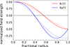 |
Fig. B.1. Comparison between br(r) and bθ(r) (Eqs. B.2 and B.3) from Broderick & Narayan (2007, dotted lines) and the polynomial fit that enforces the correct boundary conditions (full lines) as a function of the fractional radius of the magnetized zone. The fit is created such that both formalisms agree at half the strength of br(r) (dashed black line). |
Appendix C: Constraints from asteroseismology during the RGB
We used the recent asteroseismic measurements of the magnetic field strength in the radiative interior during the RGB to constrain the initial field strength at the start of the WD cooling sequence. These measurements are mostly sensitive to the radial field component averaged at the H-shell, with some additional sensitivity closer to the core (Li et al. 2022; Bhattacharya et al. 2024). Following Appendix C in Bhattacharya et al. (2024), we defined the measured squared field strength as
 (C.1)
(C.1)
which is a horizontal and radial average of the magnetic field weighted by the sensitivity kernel K(r) (for details, see Das et al. 2020 and Bhattacharya et al. 2024), with Rc the core radius. Thus, we used detected values for  from Deheuvels et al. (2023) and Hatt et al. (2024) to calibrate B0 (Eqs. B.2 and B.3 and Fig. B.1).
Appendix D: Details on the magnetic evolution
We describe in detail in this appendix the method we use to evolve magnetic fields along stellar evolution. Most of this appendix is a direct translation of the method described in Takahashi & Langer (2021).
D.1. Equations
First, we assumed that the magnetic fields we consider are weak enough not to affect the stellar structure. Thus, we decoupled the evolution of the magnetic field from that of the considered star. Additionally, for simplicity, we ignored all effects from the mean-field magnetohydrodynamic-dynamo formulation, which results in the ohmic induction equation (also Eq. 1)
 (D.1)
(D.1)
In the case of zero diffusivity, magnetic flux will be conserved in the originally magnetized mass coordinate. If there is finite diffusivity, instead, the magnetic flux evolves according to Alfvén’s theorem. Given a surface S that moves with velocity U, the magnetic flux ΦB = ∫SB ⋅ dS evolves according to
 (D.2)
(D.2)
We considered the same surface (S) as Takahashi & Langer (2021), which is a polar cap at radius rc from the center with an opening angle θc (see Takahashi & Langer 2021 Fig. 1 for an illustration of S). Additionally, we define U as the radial velocity the stellar model has at rc, i.e., U(t) = u(rc, t). Thus, inserting Eq. D.1 into Eq. D.2 and using Stokes’ Theorem results in
 (D.3)
(D.3)
where ∂S is the boundary of S. Since the magnetic field B has zero divergence, i.e., ∇ ⋅ B = 0, we can define a vector potential A such that B = ∇∧A. Since we are only interested in a poloidal magnetic field, we defined A as
 (D.4)
(D.4)
with Υℓ, m = r ∧ ∇Yℓ, m the toroidal vector spherical harmonics2 (Barrera et al. 1985), B0 the field normalization from Eq. B.2, and X such that
 (D.5)
(D.5)
 (D.6)
(D.6)
The relation between br, bθ and X follows directly from taking the curl of Eq. D.4 and comparing terms with Eqs. B.2 and B.3.
Making use of the vector spherical harmonics curl identities (Barrera et al. 1985) we can write the right hand side of Eq. D.3 as
 (D.7)
(D.7)
where f′=∂f/∂r, and the magnetic flux as
 (D.8)
(D.8)
 (D.9)
(D.9)
Notice that the only place rc comes into play in the integral is in ∂S as the distance of the surface from the center. Thus, we can rescale S to take out this dependence. This results in
 (D.10)
where quantities denoted as  are now scaled to be a unit distance away from the center. Thus, we can write the integral over the boundary of S as rc times a function that only depends on the opening angle of S. Thus,
  does not depend on time and can be pulled out of the total time derivative of ΦB. Using this, we see that X is simply the magnetic flux scaled by a constant that depends on the surface S through which the magnetic flux is defined, i.e.,
 (D.11)
Finally, combining everything, we get
 (D.12)
with ▫′ and ▫″ the first and second spatial derivatives respectively, and canceled  on both sides. Since rc is arbitrary, we leave out the subscript c and end up with the general evolution equation for the magnetic flux.
One complexity we have not discussed so far is the implicit time-dependence of r, i.e., everywhere we should replace r with r(t). This is important to consider since the left-hand side of the equation is the total time derivative of X. We solved this by applying a transformation from radius to mass coordinates. We defined mass coordinates m = (m, θ, ϕ) with
 (D.13)
instead. Since the magnetic field is confined deeply in the star, we consider the magnetic flux to be conserved (as opposed to the work of Takahashi & Langer 2021, where magnetic flux is lost by winds). Thus, we defined a maximum mass ℳ that we consider for the magnetic evolution. This mass in turn defines a time dependent maximum radius ℛ(t) via Eq. D.13:
 (D.14)
This way, our mass coordinate is independent of time, and we can discretize m as a uniform grid on which to numerically solve Eq. 1. We defined functions in m coordinates as
 (D.15)
Additionally, to transform derivatives, we used
 (D.16)
Thus, the final form of our magnetic evolution equation is
 (D.17)
We numerically solve Eq. D.17 along the evolution of the model star, starting from the end of the MS, resulting in the field profiles represented in Fig. 1.
D.2. Boundary conditions
We followed the mass coordinates enclosed in the radius ℛ(t) comprising the final WD mass (ℳ) during the full evolution, and followed the boundary conditions as in Cumming (2002) for a dipolar field:
 (D.18)
 (D.19)
which forced the magnetic field to be finite at the center and continuous with a vacuum field at the outer boundary. We used the vacuum field boundary also for the ℛ(t) boundary condition during the evolution pre WD to allow for diffusion of the magnetic field. We compared results obtained from this boundary condition to one that confines the flux in the considered zone, i.e., setting X(ℛ(t)) = 0. However, due to the magnetic fields being confined deep below the chosen boundary, the difference between these two outer boundary conditions is negligible.
To transform these equations into mass coordinates, we applied Eq. D.16 to get
 (D.20)
 (D.21)
Appendix E: Evolution of the magnetic field geometry during the RGB stage
In this appendix we provide insight into the mechanism driving the evolution of the magnetic field geometry of Scenario C, i.e., why the magnetic field in Scenario C becomes confined in a shell away from the center. First, we note that X is simply magnetic flux scaled by some constant that only depends on the choice of the surface through which the flux is defined (see Eq. D.11). The magnetic flux is bound to its mass coordinate and only evolves via diffusion (see the left panel of Fig. E.1). However, to get to br we need to multiply X by r−2 (see the middle panel of Fig. E.1), which decreases sharply above the H-shell (full black line) due to the strong density gradient present there. Thus, the resulting radial magnetic field strength br reaches its maximum close to the flux maximum (∼0.24M⊙ in this case; see the right panel of Fig. E.1). A visualization of the magnetic field geometry is represented in Fig. E.2.
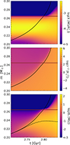 |
Fig. E.1. Evolution of Scenario C during the RGB around the H-shell (solid black line). The magnetic mass ℳC ∼ 0.26M⊙ is shown as a solid red line. Left: Contour map of the magnetic flux in log-scale as it evolves according to Eq. D.17. Middle: Contour map of r−2 in log-scale. Right: Contour map of br in log-scale as a result of multiplying the two panels above. The dashed black line shows the location of the maximum of br. |
In contrast, for the other scenarios, the flux maximum is confined below the H-shell, and thus, the strong density gradient there does not affect the magnetic field significantly.
 |
Fig. E.2. 2D slice of the magnetic field of Scenario C at the start of the WD cooling sequence. Left: Local magnetic field strength |

Appendix F: Magnetic evolution during the WD cooling sequence
Here, we discuss the evolution of the radial dependence of the magnetic field along the WD cooling sequence. Figure F.1 shows Br of Scenario C for different cooling ages. Already after 0.2Gyr (purple profile), the shape of the magnetic field has changed a lot compared to the initial profile (blue). However, the surface field strength (Fig. F.1 right panel) has not increased noticeably by that point (see also Fig. 2 for a comparison). Even after 8 Gyr, the maximum of the magnetic field is still located in a shell away from the center of the WD. This shows that the concentration of the magnetic field in a spherical shell is stable against magnetic diffusion. As a visual guide, Fig. E.2 shows a 2D slice of the magnetic field at the start of the WD cooling sequence.
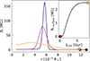 |
Fig. F.1. Evolution of Scenario C along the WD cooling sequence. Left: Br as a function of radius for three different cooling ages: tcool = 0Gyr (dark blue), tcool = 0.2Gyr (purple), and tcool = 8Gyr (yellow), with the colored circles emphasizing the current field strength at the surface. Right: Br at the surface of the WD as a function of cooling age. The three colored circles correspond to the surface field strength of the three radial profiles in the left panel. |
Appendix G: Robustness of the results
In this appendix we present additional checks to confirm that an extended magnetic field is needed during the RGB to explain the observed field strengths of magnetic WDs. First, we discuss the effect of varying the parameter rthresh (as defined in Appendix B) and afterward, the effect of stellar mass.
G.1. Impact of varying rthresh
Here, we constrained the extent of the magnetic field needed during the RGB to fit the observed field strengths on the WD cooling sequence. For this, we modified Scenario C by varying rthresh (see Appendix B). Figure G.1 shows that an rthresh ≳ 0.3 is needed to explain most observed field strengths on the WD cooling sequence. Thus, we conclude that a significant portion of the radiative interior during the RGB has to be strongly magnetized, extending much beyond the H-shell.
G.2. Impact of the stellar mass
To characterize the mass dependence of the magnetic emergence time on WD surfaces, we show the same plot as Fig. 2, but for initial masses of 1.3M⊙ (Fig. G.2) and 1.8M⊙ (Fig. G.3), representing typical lower and upper mass bounds of magnetized RGs that used to have a convective core during the MS (Hatt et al. 2024). While there are small shifts in both the emergence time and the maximum field strength reached, these changes are not large enough to change our results as stated in Sect. 3. Thus, we validated our conclusion that an extended radial field profile is needed on the RGB to explain the observed WD surface field strengths from asteroseismic constraints on the RGB, independently of the initial mass of the star.
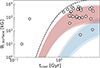 |
Fig. G.2. Same as Fig. 2 but for a stellar model with initial mass of 1.3M⊙. The field evolutions for the 1.5M⊙ model from Fig. 2 are shown in grey for easy comparison. |
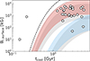 |
Fig. G.3. Same as Fig. 2 but for a stellar model with initial mass of 1.8M⊙. The field evolutions for the 1.5M⊙ model from Fig. 2 are shown in grey for easy comparison. |
All Figures
|
Fig. 1. Considered magnetic field configurations at different evolutionary stages of a typical 1.5 M⊙ star. The central field strengths are set such that asteroseismic detections of all three fields would measure 100 kG during the RGB stage (see Appendix C). Left panel: Scenarios A (dark blue line) and B (light blue line) are created by the convective core during the MS stage and start evolving as a large-scale stable field at the end of the MS. Middle panel: Magnetic fields during the RGB stage when the typical oscillation frequency of the star reaches 150 μHz. The two fields for Scenarios A and B are now buried below the hydrogen-burning shell (dashed line). Scenario C (red line) starts its evolution here and fills the entire radiative interior. Right panel: Magnetic field configurations for all three scenarios at the start of the WD cooling sequence. The blue-shaded region corresponds to the radial extent of the WD mass at different evolutionary stages. |
| In the text | |
|
Fig. 2. Radial surface field strength as a function of the cooling age of the WD for Scenarios B (blue) and C (red). The shaded regions show the evolution for varying field strengths on the RGB between 10 kG (bottom) and 200 kG (top), the range detected in Hatt et al. (2024). The dashed line shows the emergence of the strongest detected RGB field of 600 kG (Deheuvels et al. 2023) and places a lower limit on the FFS emergence timescale. The white circles show detected magnetic WDs from the Bagnulo & Landstreet (2022) and Moss et al. (2025) samples in the mass range [0.5 − 0.64] M⊙. |
| In the text | |
|
Fig. B.1. Comparison between br(r) and bθ(r) (Eqs. B.2 and B.3) from Broderick & Narayan (2007, dotted lines) and the polynomial fit that enforces the correct boundary conditions (full lines) as a function of the fractional radius of the magnetized zone. The fit is created such that both formalisms agree at half the strength of br(r) (dashed black line). |
| In the text | |
|
Fig. E.1. Evolution of Scenario C during the RGB around the H-shell (solid black line). The magnetic mass ℳC ∼ 0.26M⊙ is shown as a solid red line. Left: Contour map of the magnetic flux in log-scale as it evolves according to Eq. D.17. Middle: Contour map of r−2 in log-scale. Right: Contour map of br in log-scale as a result of multiplying the two panels above. The dashed black line shows the location of the maximum of br. |
| In the text | |
|
Fig. E.2. 2D slice of the magnetic field of Scenario C at the start of the WD cooling sequence. Left: Local magnetic field strength |
| In the text | |
|
Fig. F.1. Evolution of Scenario C along the WD cooling sequence. Left: Br as a function of radius for three different cooling ages: tcool = 0Gyr (dark blue), tcool = 0.2Gyr (purple), and tcool = 8Gyr (yellow), with the colored circles emphasizing the current field strength at the surface. Right: Br at the surface of the WD as a function of cooling age. The three colored circles correspond to the surface field strength of the three radial profiles in the left panel. |
| In the text | |
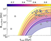 |
Fig. G.1. Same as Scenario C in Fig. 2 but with a varying rthresh. |
| In the text | |
|
Fig. G.2. Same as Fig. 2 but for a stellar model with initial mass of 1.3M⊙. The field evolutions for the 1.5M⊙ model from Fig. 2 are shown in grey for easy comparison. |
| In the text | |
|
Fig. G.3. Same as Fig. 2 but for a stellar model with initial mass of 1.8M⊙. The field evolutions for the 1.5M⊙ model from Fig. 2 are shown in grey for easy comparison. |
| In the text | |
Current usage metrics show cumulative count of Article Views (full-text article views including HTML views, PDF and ePub downloads, according to the available data) and Abstracts Views on Vision4Press platform.
Data correspond to usage on the plateform after 2015. The current usage metrics is available 48-96 hours after online publication and is updated daily on week days.
Initial download of the metrics may take a while.