| Issue |
A&A
Volume 708, April 2026
|
|
|---|---|---|
| Article Number | A178 | |
| Number of page(s) | 14 | |
| Section | The Sun and the Heliosphere | |
| DOI | https://doi.org/10.1051/0004-6361/202659310 | |
| Published online | 03 April 2026 | |
The role of ambipolar heating in the energy balance of solar prominences
1
Departament de Física, Universitat de les Illes Balears, E-07122 Palma de Mallorca, Spain
2
Institut d’Aplicacions Computacionals de Codi Comunitari (IAC3), Universitat de les Illes Balears, E-07122 Palma de Mallorca, Spain
★ Corresponding author: This email address is being protected from spambots. You need JavaScript enabled to view it.
Received:
4
February
2026
Accepted:
13
March
2026
Abstract
Solar prominence threads are typically located around magnetic dips, where cold and dense plasma is suspended against gravity in the hot corona due to the upward magnetic force. Because prominences are partially ionized, ambipolar diffusion has the capacity to deposit part of the energy of their non-force-free magnetic field into the plasma. This ambipolar heating could therefore play a role in the energy balance of prominences. In this proof-of-concept work, we explore the effect of ambipolar diffusion in one-dimensional models that satisfy both mechanical equilibrium and energy balance. The magnetic configuration is based on the classic Kippenhahn–Schlüter model, incorporating a sheared magnetic field. The temperature profile along the magnetic field was computed numerically by balancing radiative losses, thermal conduction, and ambipolar heating. The resulting models are consistently comprised of a cold, dense, partially ionized thread with prominence core conditions, a very thin prominence-corona transition region, and an extended, hot, fully ionized region with coronal conditions. In addition to providing heating that partly compensates for radiative losses, ambipolar diffusion also gives rise to stationary flows associated with the gravitational drainage of neutrals in the partially ionized region. Here, we investigate how the length of the cold threads depends on the central temperature, central pressure, magnetic field strength, and shear angle. We show that thread lengths compatible with observational results can be obtained for realistic values of these parameters. Finally, we demonstrate that ambipolar diffusion plays a relevant role in this simple configuration, indicating that this effect should be incorporated into more elaborate multidimensional models and simulations.
Key words: magnetohydrodynamics (MHD) / Sun: atmosphere / Sun: corona / Sun: filaments / prominences
© The Authors 2026
 Open Access article, published by EDP Sciences, under the terms of the Creative Commons Attribution License (https://creativecommons.org/licenses/by/4.0), which permits unrestricted use, distribution, and reproduction in any medium, provided the original work is properly cited.
This article is published in open access under the Subscribe to Open model. This email address is being protected from spambots. You need JavaScript enabled to view it. to support open access publication.
1. Introduction
Solar prominences are one of the most intriguing objects in the solar atmosphere. They consist of masses of relatively cool and dense plasma suspended in the corona. Although they reside in the corona, their plasma properties are more similar to those in the chromosphere (see, e.g., Vial & Engvold 2015). An important property of the prominence plasma is that it is partially ionized (see, e.g., Heinzel et al. 2024). Prominences are composed of numerous long and thin ribbons, called threads, which are only seen in high-resolution observations (see, e.g., Lin 2011). These threads presumably outline the prominence magnetic structure, whose field lines are anchored at the photosphere (see, e.g., Martin 2015). The threads are believed to reside in magnetic dips, which allow the dense prominence plasma to be supported against gravity (e.g., Anzer & Heinzel 2007), although this idea has also been challenged (Karpen et al. 2001).
Explaining how prominences and their threads are formed in the coronal medium is a complicated topic and several different mechanisms might be involved (see Karpen 2015; Zhou 2025). However, there is a growing consensus that the key process that allows the condensation of the cool prominence plasma is related to thermal instability (for a recent review, see Keppens et al. 2025, and references therein). In this context, the role of partial ionization in the formation through the evaporation-condensation process has been investigated by Jerčić et al. (2025). Once formed, prominences can remain in a relative stable global state for long periods of time before their eventual disappearance (see Parenti 2014). The present paper does not deal with the formation of prominences. Instead, we focus on studying their equilibrium.
There is a rich store of literature on prominence equilibrium models. The mechanical equilibrium is a problem well understood, as it is established that the upward force produced by the magnetic field is required to compensate for gravity (see Gibson 2018). A pioneering work in this area is the classic paper by Kippenhahn & Schlüter (1957), hereafter referred as the K-S model, based on the construction of magnetohydrostatic equilibrium. In the K-S model, the weight of the prominence plasma produces a shallow dip in a nearly horizontal magnetic field. Although many subsequent papers have been based on the K-S model, it represents the most simplified approach and more elaborate models exist in the literature (see, e.g., Kuperus & Raadu 1974; Ballester & Priest 1987; Hood & Anzer 1990; Heinzel & Anzer 2001; Low & Petrie 2005; Blokland & Keppens 2011, to name a few). Some applications of the K-S model include the study of prominence oscillations (e.g., Oliver et al. 1992, 1993; Anzer 2009) and instabilities (Hillier et al. 2010).
Contrary to the mechanical equilibrium, the energy balance is a problem not completely solved (see, e.g., Gilbert 2015). Although such a balance must necessarily result from the interplay between cooling, heating, and thermal conduction, their relative importance and, particularly, the nature of the heating remain under study (see Anzer & Heinzel 1999). As prominences are suspended in the corona, illumination from the photosphere and the surrounding corona is an important heating source (see Poland & Anzer 1971; Heasley & Mihalas 1976; Heinzel et al. 2025). However, radiative equilibrium models obtained by solving the full non-local thermodynamic equilibrium (NLTE) radiative-transfer problem typically produce slightly lower equilibrium temperatures than those expected in prominence cores (see, e.g., Heinzel et al. 2010; Heinzel & Anzer 2012). Recently, Gunár et al. (2025) computed net radiative cooling rates from 1D NLTE isothermal and isobaric models (see also Heinzel et al. 2025). These net rates result from the combined effects of radiative cooling and radiative heating. According to Gunár et al. (2025), a net loss of energy occurs for typical conditions in prominence cores. Their results suggest that although radiative heating is most likely the dominant heating mechanism in prominences, another complementary heating could be necessary to completely balance the net energy losses.
Several heating mechanisms may be acting in the coronal medium (see, e.g., Mandrini et al. 2000; Arregui & Van Doorsselaere 2024). In the context of prominences, some works have used parametrized forms of the heating aiming to represent different processes in a simplified way without explicitly solving the underlying physics (see, e.g., Brughmans et al. 2022). A potential heating source is related to the dissipation of magnetohydrodynamics (MHD) waves (e.g., Pécseli & Engvold 2000; Parenti & Vial 2007; Soler et al. 2016; Melis et al. 2021; Hashimoto et al. 2023). Since the prominence plasma is partially ionized, another possibility is the dissipation of currents by ambipolar diffusion. This type of heating mechanism has been investigated in the chromosphere (e.g., Goodman 2004; Khomenko & Collados 2012; Martínez-Sykora et al. 2017; Stepanov et al. 2024). However, its importance in the energy balance of prominences has not been examined yet.
Prominence equilibrium models that simultaneously satisfy both mechanical equilibrium and energy balance have been explored in the literature using different approaches (e.g., Poland & Anzer 1971; Low 1975; Milne et al. 1979; Low & Wu 1981; Degenhardt & Deinzer 1993; Schmitt & Degenhardt 1995; Vigh et al. 2018, to name a few). Our goal is to construct this kind of model, but which would include the effect of ambipolar diffusion. To this end, we deliberately adopted a simple approach based on the use of a modified K-S configuration as way of testing the importance of ambipolar heating in the energy balance. The currents associated with the non-force-free magnetic field of the K-S model are susceptible to be dissipated by ambipolar diffusion, which would cause the deposition of magnetic energy into the plasma. This kind of heating would affect the energy balance and the relative importance of radiative losses and thermal conduction.
The method we use to construct the models is based on those of Terradas et al. (2021) and Melis et al. (2023), which is restricted to finding one-dimensional (1D) equilibria that satisfy the energy balance equation along a magnetic field line. In Terradas et al. (2021) an arbitrarily imposed uniform heating was used and the magnetic field was prescribed instead of being computed from the balance of forces. Melis et al. (2023) extended the method by considering a nonuniform heating resulting from the dissipation of Alfvén waves. Melis et al. (2023) implemented a numerical scheme in which the Alfvén wave equation and the energy balance equation were solved iteratively until convergence to a self-consistent equilibrium was achieved. However, Melis et al. (2023) also prescribed the magnetic field. Here, we followed an iterative strategy as in Melis et al. (2023), but with two important differences. On the one hand, we included ambipolar diffusion as a heating mechanism instead of wave heating. On the other hand, we coupled the balance of forces with the energy equation. As a result, the obtained models satisfy both the mechanical equilibrium and energy balance, while including ambipolar diffusion in a consistent manner.
This paper is structured as follows. Section 2 includes an explanation of the method and the self-consistent approach. The results of the computed models are presented in Sect. 3. Finally, some general conclusions are given in Sect. 4. Additionally, Appendix A discusses the convergence of the numerical method used to compute the models. Appendix B includes a comparison of our results with those of the related work by Milne et al. (1979).
2. Method
2.1. Basic equations for partially ionized plasma
In this work, we used the single-fluid MHD equations for partially ionized plasmas (e.g., Ballester et al. 2018). The basic equations are
 (1)
(1)
 (2)
(2)
![Mathematical equation: $$ \begin{aligned}&\frac{\partial \boldsymbol{B}}{\partial t} = \nabla \times \left( \boldsymbol{v} \times \boldsymbol{B} \right) +\nabla \times \Bigl \{ \eta _{\rm A} \left[ \left(\nabla \times \boldsymbol{B}\right) \times \boldsymbol{B} \right]\times \boldsymbol{B} \Bigr \}, \end{aligned} $$](/articles/aa/full_html/2026/04/aa59310-26/aa59310-26-eq3.gif) (3)
(3)
 (4)
(4)
 (5)
(5)
with  the material derivative. These equations are, respectively, the continuity equation, the momentum equation, the induction equation, the energy equation, and the solenoidal condition of the magnetic field. The symbols in these equations have their usual meaning: v is the velocity, p is the gas pressure, ρ is the mass density, μ0 is the magnetic permeability, B is the magnetic field, g is the acceleration of gravity, ηA is the ambipolar diffusion coefficient, γ is the adiabatic index, and ℒ the heat-loss function, which encloses all sources and sinks of energy, such as radiative cooling, thermal conduction, and ambipolar heating. This is elaborated upon later.
The relation between pressure and temperature, T, can be written with the ideal gas law, namely,
 (6)
(6)
where N is the total number density and kB is Boltzmann’s constant. We considered a partially ionized plasma composed of hydrogen and helium. The total number density is computed as
 (7)
(7)
where nβ denotes the number density of the different species β of the plasma. The species considered are electrons (e), protons (p), neutral hydrogen (H), neutral helium (HeI), singly ionized helium (HeII) and doubly ionized helium (HeIII). The number densities of the various species can be computed as functions of total mass density, ρ, as
 (8)
(8)
 (9)
(9)
 (10)
(10)
for j = I, II, and III, where A is the helium to hydrogen abundance ratio, mp is the proton mass, and ξβ denotes the mass fraction of the corresponding species, β. In turn, owing to charge conservation, the electron number density satisfies
 (11)
(11)
We considered A = 0.1, which means an abundance of helium of 10% with respect to that of hydrogen. Therefore, N can be reformulated as
 (12)
(12)
These definitions allow us to rewrite Eq. (6) in the usual form,
 (13)
(13)
where R = kB/mp is the ideal gas constant and  is the mean atomic weight, which in our case is written down as
 (14)
(14)
The mass fractions of the various species can be used to denote their ionization degree. Hence, ξp is used to denote the hydrogen ionization, while ξHeII and ξHeIII denote the two different states of helium ionization. In order to set ξp, we used the values in Table 1 from Heinzel et al. (2015) for an altitude of 20,000 km above the photosphere, which are obtained from NLTE computations in 1D prominence slabs1. The values of the table were interpolated and for T ≥ 2 × 10⁴ K we considered full ionization of hydrogen, i.e., ξp = 1. However, to our knowledge, no similar NLTE computations are currently available in the case of helium. To circumvent this limitation, we adopted a simplified LTE approach using the Saha equation. The expressions of ξHeII and ξHeIII are
 (15)
(15)
 (16)
(16)
where 𝒩HeII and 𝒩HeIII represent the ratio between the number density in the corresponding ionization state and that in the previous ionization stage. The ratios can be computed as
 (17)
(17)
 (18)
(18)
where ZHeI = ZHeIII = 1 and ZHeII = 2 are the partition functions of the ionization stages, h is Planck’s constant, me is the electron mass, and χHeI = 24.6 eV and χHeII = 54.4 eV are the corresponding ionization energies.
The ionization fractions of helium in both ionization states are coupled with the hydrogen ionization fraction through the electron number density (Eq. (11)). We solved the coupled system and computed the ionization fractions of both ionized helium species as functions of the temperature and pressure. Figure 1 illustrates how the ionization fractions of all the considered species vary as functions of T for a prescribed value of p. For low temperatures, hydrogen is partially ionized, while helium is neutral. As T increases, the progressive ionization of hydrogen follows the NLTE results of Heinzel et al. (2015), whereas the ionization of helium follows the LTE result from the Saha equation. For T ≈ 11 000 K singly ionized helium becomes the dominant helium state, while for T ≈ 23 000 K doubly ionized helium becomes dominant. Full ionization of helium is reached at T ≈ 30 000 K.
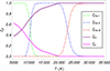 |
Fig. 1. Ionization fractions of hydrogen and helium for p = 5 × 10⁻³ Pa as functions of the temperature, T. |
In Eq. (3), we consider the nonideal ambipolar diffusion, which is related with ion-neutral collisions, but other effects such as Ohmic diffusion, Hall’s term, and the battery term have been dropped for simplicity (see, e.g., Khomenko et al. 2014; Ballester et al. 2018). Previous results in Melis et al. (2023) indicate that ambipolar diffusion is the dominant effect in prominence conditions. The ambipolar diffusion coefficient, ηA, in a partially ionized hydrogen-helium plasma takes the expression (see Zaqarashvili et al. 2013; Soler et al. 2015):
 (19)
(19)
where αβ is the total friction coefficient of species β (accounting for collisions of this particular species with all the others) and αββ′ = αβ′β is the symmetric friction coefficient for collisions between species β and β′. The total friction coefficients are computed as
 (20)
(20)
If both species are charged, the friction coefficient (e.g., Spitzer 1962; Braginskii 1965) is
 (21)
(21)
where mββ′ = mβmβ′/(mβ + mβ′) is the reduced mass, e is the electron charge, ϵ0 is the electrical permittivity, and Λββ′ is the Coulomb logarithm, expressed as
 (22)
(22)
If at least one of the colliding species is neutral, the friction coefficient is the approximation of small drift velocity becomes (e.g., Braginskii 1965; Chapman & Cowling 1970; Draine 1986)
 (23)
(23)
where σβn is the collisional cross section, whose values in the context of the solar atmosphere can be found in the works of Vranjes & Krstic (2013) and Wargnier et al. (2022), for instance.
2.2. Mechanical equilibrium
We used a Cartesian coordinate system. We assumed that gravity points in the negative z-direction, so that  , with g the surface acceleration of gravity assumed constant. Seeking an equilibrium, we imposed ∂/∂t = 0 in the MHD Eqs. (1)–(4). Additionally, we assumed that all variables only vary along the x-direction. Under these conditions, the problem of finding an equilibrium is analogous to the classic K-S configuration, modified here by the presence of ambipolar diffusion owing to partial ionization. The effect of gravity should produce a curved magnetic field (i.e., a dip), where the prominence material can be supported. Therefore, we found that the horizontal components of the magnetic field, Bx and By, are both constant, so that these two components can be expressed in terms of a uniform horizontal magnetic field strength, B0, and a shear angle ϕ = arctan(By/Bx), namely,
 (24)
(24)
 (25)
(25)
In turn, the vertical component of the magnetic field, Bz, follows the typical K-S form, namely,
 (26)
(26)
where p0 is the pressure at the center of the magnetic dip (located at x = 0) and the function f(x) (see Poland & Anzer 1971) is
 (27)
(27)
We note that at the current stage,  and T are still unknown, so that f(x) cannot be explicitly computed yet. The pressure and density again follow the K-S solution, namely,
 (28)
(28)
 (29)
(29)
The density is nonuniform, owing to the accumulation of the prominence mass around the dipped part of the field line. In addition, a nonuniform pressure is also required to preserve the force balance along the magnetic field line.
While there are no equilibrium flows in the classic K-S equilibrium (i.e., it is static), such flows appear when ambipolar diffusion is included, so that the equilibrium is stationary (see also Bakhareva et al. 1992). Assuming vx = 0, the y- and z-components of the equilibrium velocity are
 (30)
(30)
 (31)
(31)
The result that vy and vz are both proportional to ηA plainly shows that these equilibrium flows are driven by ambipolar diffusion. The role of these flows, especially that of the vertical one, is explored later in this work. We note that the general case with vx ≠ 0 is considerably more complicated (see, e.g., Tsinganos & Surlantzis 1992). The main reason for adopting vx = 0 is that we are seeking equilibrium solutions that are essentially modified versions of the classic K-S model. If vx ≠ 0, terms proportional to vx and its spatial derivative appear in all the governing equations, introducing effects such as the enthalpy flux in the energy balance equation. Since these kinds of siphon flows can be obtained in time-dependent simulations (see, e.g., Xia et al. 2011; Donné & Keppens 2024), relaxing the condition vx = 0 would be an interesting extension of this study, which could lead to the computation of a different family of solutions. This investigation is left to future works.
2.3. Energy balance
The equilibrium obtained in the previous subsection is still incomplete. The modified K-S solution depends on the function f(x) that, in turn, requires  and T to be known. The mean atomic weight can be computed from Eq. (14). However, knowledge of the ionization state of the plasma is needed, which depends on the temperature. Therefore, computing f(x) ultimately reduces to computing the temperature profile. To this end, we solved the energy balance condition.
The heat-loss function, ℒ, on the right-hand side of Eq. (4) generally takes the expression,
 (32)
(32)
where QA is the ambipolar heating,  is the heat flux due to thermal conduction, with
  the thermal conductivity tensor, Lrad. represents the energy losses due to radiative cooling, and C might represent other heating sources, such as viscous and/or Ohmic heating, which we ignore here.
The ambipolar heating was calculated using the Joule heating function that accounts for the dissipation of perpendicular electric currents (e.g., Khomenko & Collados 2012), namely,
 (33)
(33)
where J⊥ is the perpendicular component of the current density with respect to the magnetic field direction. Since the equilibrium magnetic field in the K-S solution is not force free, there is necessarily a nonzero current in the equilibrium. We then find
 (34)
(34)
After some algebra, we easily arrive at an expression for the heating rate, namely,
 (35)
(35)
Therefore, ambipolar diffusion of the magnetic field continuously provides a heating input to the plasma. For an equilibrium to exist, this heating needs to be compensated via thermal conduction and radiative cooling.
Regarding thermal conduction in a partially ionized plasma, the conductivity of charges is dominated by the component parallel to the magnetic field, while that of neutrals is essentially isotropic (see, e.g., Soler et al. 2015). Consequently, the divergence of the heat flux in our configuration is reduced to
 (36)
(36)
with the effective thermal conductivity, κeff., being approximated as
 (37)
(37)
where κ∥, c and κn are the parallel component of the conductivity of charges and the isotropic neutral conductivity, respectively. The role of the charges thermal conductivity is influenced by orientation of the magnetic field through the factor Bx/|B|, since only the parallel component is relevant. These conductivities are computing by adding the contributions of the various species, namely,
 (38)
(38)
 (39)
(39)
where the species-related conductivities are computed as
 (40)
(40)
for β = e, p, HeII, and HeIII, with
 (41)
(41)
for β = H and HeI. In these expressions, αββ denotes the friction coefficient for internal self-collisions of species, β, while all the other quantities are already defined.
Now, we go on to discuss the treatment of radiative losses. In principle, the net losses should be computed from the combined effects of radiative cooling and radiative heating, as done recently by Gunár et al. (2025) using NLTE calculations. The net losses tabulated in Gunár et al. (2025) depend on the location of the plasma element with respect to the source of illumination, that is, the depth within the prominence. However, the numerical procedure used here to generate models, based on the one from Melis et al. (2023), requires the cooling rate to be expressed as a function of the local plasma properties alone. The implementation of the tables from Gunár et al. (2025) requires a modification of the numerical scheme of Melis et al. (2023) that is beyond the aims of the present paper and left to a forthcoming work. Therefore, we used a simplified treatment to approximate the net radiative losses. The adopted radiative cooling function takes the form of
 (42)
(42)
This expression can be rewritten in terms of the total mass density as
 (43)
(43)
where Λ(T) in this and the previous expression is a piecewise function that depends on the temperature. Here, we use the SPEX_DM curve from Hermans & Keppens (2021)2. This is, essentially, an optically thin cooling curve modified with a special treatment for low temperatures (T < 104 K), as described in Schure et al. (2009). This and other similar curves have recently been used in prominence simulations (see, e.g., Brughmans et al. 2022; Jerčić et al. 2025, among others). As explained by Heinzel et al. (2025), the NLTE net cooling rates may deviate significantly from optically thin calculations and so, caution is needed on this matter.
Formally, the condition of the energy balance is
 (44)
(44)
which results in a complicated second-order nonlinear differential equation for T that needs to be solved numerically. The full expression is omitted here for the sake of simplicity. We note that, apart from the fundamental constants, all physical quantities are spatially dependent in the model, with the exception of the horizontal component of the magnetic field and the shear angle.
2.4. Numerical solution and self-consistent strategy
We considered a single magnetic field line of length, L. We used the coordinate s to denote length along the magnetic field line, with the center located at s = 0 and the end at s = ±L/2. The parametric equations for the magnetic field lines are
 (45)
(45)
If the horizontal component dominates, as expected, then Bz ≪ B0 and |B|≈B0. Therefore, the coordinates x and y are almost directly proportional to s, since Bx and Bx are both uniform. The parametric representation of the magnetic field line is
 (46)
(46)
 (47)
(47)
 (48)
(48)
where x0, y0 and z0 are arbitrary constants, so that x0 = y0 = z0 = 0 can be imposed with no loss of generality. We note that the actual height of the field line is irrelevant since the K-S model is invariant in the vertical direction.
We used Wolfram Mathematica to numerically solve the energy balance condition (Eq. (44)). The integration was performed with the module NDSolve, which adapts the spatial resolution in order to minimize the numerical error. The numerical integration was performed in two stages: first from x = 0 to x = xmax./2 and then from x = 0 to x = −xmax./2, where xmax. is the maximum value of the x coordinate that corresponds with s = L/2. The two solutions were joined together and the complete profile was constructed. In all cases, we considered a total length of L = 100 Mm.
We imposed the same boundary conditions as in Terradas et al. (2021) and Melis et al. (2023). We prescribed a central temperature, T0, and required the temperature to be at its minimum at the center, namely,
 (49)
(49)
 (50)
(50)
In addition, Terradas et al. (2021) showed that an additional restriction must be satisfied at the center for an equilibrium to exist under such conditions, namely,
 (51)
(51)
so that Lrad. > QA at the center. If QA > Lrad., the heating would be too intense, making it impossible the existence of an equilibrium.
Equilibrium solutions were studied considering four parameters: the central pressure, p0, the horizontal magnetic field strength, B0, the shear angle, ϕ, and the central temperature, T0. The considered ranges of values for those parameters are: from 2 × 10⁻³ Pa < p0 < 1.5 × 10⁻² Pa, 4 G < B0 < 20 G, 0° < ϕ < 90°, and 7000 K < T0 < 10 000 K. The central temperatures and pressures were chosen to be consistent with those expected in prominence cores, while the magnetic field strength corresponds to that seen in quiescent prominences (see, e.g. Gibson 2018). Importantly, these four parameters are not completely independent from each other regarding the existence of an equilibrium solution, so that it was not possible to compute equilibria for certain combinations of parameters. This is explored later in this paper.
In a similar way as the issue described in Melis et al. (2023) for the case of Alfvén wave heating, the computation of equilibrium models that incorporated ambipolar heating posed a circular problem. The heating rate depends on the magnetic field, temperature, and other quantities through Eq. (35). However, the temperature is obtained by solving the energy balance condition (Eq. (44)), which needs the heating rate to be known in advance. We solved this circular problem with an iterative strategy. First, we selected particular values of B0, p0, ϕ, and T0 for which the self-consistent model is to be computed. The iterative method as initialized by solving Eq. (44) with no ambipolar heating (QA = 0). An initial temperature profile was obtained in such a way, which allowed the computation of the vertical magnetic field (Eq. (26)), the pressure (Eq. (28)), and the density (Eq. (29)) profiles. With these initial profiles, the ambipolar heating rate was computed (Eq. (35)), completing the first iteration. Then, in the second iteration, the energy balance condition was again solved, but this time using the ambipolar heating rate computed in the previous iteration. Furthermore, the profiles for temperature, vertical magnetic field, pressure, and density were updated, allowing for the computation of another ambipolar heating rate, and so on.
The profiles obtained after every iteration would be slightly different compared to those of the previous iteration. To quantify the difference from iteration to iteration, we used the L2 relative error norm of the temperature profile, since it is the one computed from the energy balance condition. The error estimation, ε, is computed with the L2 error norm as
 (52)
(52)
where Ti(x) and Ti − 1(x) are the temperature profiles for the i-th iteration and the previous iteration, respectively. We assume that a self-consistent equilibrium model is achieved when ε < ε0, where ε0 is a prescribed small tolerance. We used ε0 = 10−7. The iterative process was repeated until the convergence criterion is satisfied. As mentioned before, for some combination of parameters the constraint of Eq. (51) cannot be enforced. This causes the convergence criterion to be unachievable, even after many iterations. In those cases, it was not possible to compute an equilibrium model. The relevance of the spatial resolution and the effect of the constraint of Equation (51) are explored in Appendix A.
3. Results
3.1. Properties of a reference model
We start by presenting the results of a reference model computed using a particular set of parameters, namely, T0 = 8000 K, p0 = 5 × 10⁻³ Pa, B0 = 10 G, and ϕ = 88°. A visualization of the magnetic field line obtained in this configuration is displayed in Fig. 2, which shows the formation of a dip where the dense prominence plasma is supported.
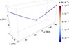 |
Fig. 2. Visualization in 3D of the magnetic dip obtained for the reference model with T0 = 8000 K, p0 = 5 × 10⁻³ Pa, B0 = 10 G, and ϕ = 88°. The color gradient denotes the variation of the density along the magnetic field line. Note: the axes are not presented to scale. |
Figure 3 shows the profiles along the magnetic field line of temperature, density, pressure, mean atomic weight, vertical component of the magnetic field, ambipolar diffusion coefficient, y- and z-components of the velocity, and ambipolar heating rate. The temperature profile (Fig. 3a) has a shape similar to the profiles presented in Terradas et al. (2021) and Melis et al. (2023), even though these previous works considered very different heating mechanisms: Terradas et al. (2021) assumed an arbitrary constant heating and Melis et al. (2023) considered heating by Alfvén waves. The profile can be understood as formed by three different regions: a central cool region with an almost parabolic shape that represents the cold prominence thread; a sharp increase of the temperature by two orders of magnitude in a very thin prominence-corona transition region (PCTR); and, finally, an extended external region where the temperature increase is smoother, reaching typical coronal temperatures of ∼8.5 × 10⁵ K. The length of the cold thread, denoted by a, is computed as in Melis et al. (2023) by detecting the location of the two PCTR that symmetrically surround the cold region. Due to the considered boundary conditions, the profile of temperature and those of the other physical quantities are symmetric or antisymmetric with respect to s = 0. For this particular model, we find a ≈ 2.56 Mm, which is a very small fraction of the total length of the magnetic field line (L = 100 Mm), but agrees well with the thread lengths reported in observations (e.g., Lin 2011).
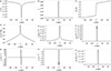 |
Fig. 3. Equilibrium profiles along the magnetic field line for the reference model: a) temperature, b) mean atomic weight, c) z-component of the magnetic field, d) pressure, e) density, f) ambipolar diffusion coefficient, g) y-component of the velocity, h) z-component of the velocity, and i) ambipolar heating rate. Results for T0 = 8000 K, p0 = 5 × 10⁻³ Pa, B0 = 10 G and ϕ = 88°. The vertical dashed red lines mark the location of the cool and dense prominence thread of a length, a ≈ 2.56 Mm, as this the distance between the two lines. |
The mean atomic weight, represented in Fig. 3b, is computed with Eq. (14). Its behavior is inverse to that of the temperature. In the cool central region,  reaches its maximum value of 0.86, approximately, which corresponds to a partially ionized plasma with ξp ≈ 0.5, ξHeII ≈ 10−4, and ξHeIII ≈ 0. This means that at the thread core, half the hydrogen is ionized, while almost all helium is neutral. In the PCTR, there is a sharp decrease of
  , related with the fast ionization of both hydrogen and helium, as well as
  in the extended coronal region. Such a value corresponds to a fully ionized hydrogen-helium plasma. A closed-up view of the transition from partial ionization to full ionization is displayed in Fig. 4a. The ionization of hydrogen progressively increases with s and reaches its complete ionization at s ≈ 1.28 Mm, within the PCTR. Conversely, the ionization of helium happens in a much thinner region. The fraction of singly ionized helium, ξHeII, peaks within the PCTR and then decreases sharply when doubly ionized helium becomes the dominant helium state. Helium reaches complete ionization at s ≈ 1.29 Mm, shortly after the location where complete ionization of hydrogen happens. We recall that the ionization of helium is computed here in a approximate manner with the Saha equation, so that the profiles of ξHeII and ξHeIII might be somewhat different in more general approaches.
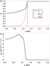 |
Fig. 4. Close-up views of some quantities of the reference model around the cold thread and the PCTR: a) Mass fractions of protons (ionized hydrogen), singly ionized helium, and doubly ionized helium. b) Ambipolar diffusion coefficient. Only half the domain with s ≥ 0 is displayed due to the symmetry of the profiles. The discontinuous derivatives of the ambipolar diffusion coefficient are caused by the first-order interpolation used to implement the hydrogen ionization degree from the tabulated values in Heinzel et al. (2015). |
The vertical component of the magnetic field, computed from Eq. (26), is shown in Fig. 3c. We find that Bz > 0 for s > 0 and Bz < 0 for s < 0, so that the profile is antisymmetric with respect to s = 0, where Bz = 0. This results in the formation of the magnetic dip. The profile has a sharp increase (decrease) in the PCTR and a smooth increase (decrease) in the outermost region. At the ends of the magnetic field line, where Bz is maximum, we find Bz ≈ ±0.35 G, which is two orders of magnitude below the strength of the horizontal component, B0. Therefore, the dip produced by the effect gravity is very shallow. Using the expression for the z-coordinate of the magnetic field line (Eq. (48)) and setting z0 = 0 as a reference, we find that z ≈ 1.5 Mm at s = L/2, which confirms that the depth of the dip is much smaller than the length of the magnetic field line.
The pressure profile is calculated from Eq. (28) and plotted in Fig. 3d. The pressure has its maximum located at the center. Then, it decreases sharply in the PCTR and in a gentler way in the coronal region, although the decrease in the outermost region with respect to the value at the center is only a small percentage. This can be explained by the fact that the variation of p is proportional to Bz2, and Bz itself takes small values, as already discussed. In turn, the density profile is computed from Eq. (29) and represented in Fig. 3e. As in the case of the pressure, the density is at its maximum at the center, with a value of ρ ≈ 5 × 10⁻¹¹ kg m−3, and decreases as we move toward the coronal part, where ρ ∼ 10−13 kg m−3. The shape of the density profile seems to mimic that of the temperature but with an inverse behavior. The magnetic field line displayed in Fig. 2 has been colored according to the values of the density. The three distinct regions discussed before are clearly shown along the magnetic field line: the dark red region around the dip corresponding to the cold and dense prominence thread, the light blue region denoting the narrow PCTR, and the dark blue representing the evacuated part of the domain matching coronal conditions.
The ambipolar diffusion coefficient, ηA, is plotted in Fig. 3f. It has a null value in the coronal region, where the plasma is fully ionized. In the cold central region, it has two relative maxima slightly displaced from the center. This shape agrees with the models computed in Melis et al. (2023). The maximum value of the coefficient is ηA ≈ 1014 m2 s−1 T−2, which is an order of magnitude above the values computed in previous works where the plasma was considered to be composed of hydrogen alone (see Melis et al. 2021, 2023). Here, the effect of helium is included and it has an important contribution to the ambipolar diffusion coefficient. The important role of helium for accurately computing ηA was discussed by Zaqarashvili et al. (2013) in the context of the chromosphere. A detailed view of ηA in the cold central region is represented in Fig. 4b, where the location of the maximum of ηA is seen to correlate well with the location where helium begins to ionize (see Fig. 4a). The sharp decrease of ηA within the PCTR, owing to the fact that the plasma gets fully ionized there, is also clearly visible.
The y- and z-components of the equilibrium flow velocity are represented in Figs. 3g and 3h, respectively. Both velocities are caused by ambipolar diffusion and depend on the ambipolar diffusion coefficient, as seen in Eqs. (30) and (31). The y-component is antisymmetric with respect to the thread center, being positive for s < 0 and negative for s > 0, taking a maximum value of vy ≈ ±200 m s−1. This means that vy represents a converging flow that is essentially directed along the magnetic field lines, owing to the large shear angle considered in this model. Despite the presence of this converging flow, the equilibrium density does not change in time. The reason for this result resides in the role of the z-component of the velocity. The vertical component of the equilibrium flow takes negative values within the thread, which means that vz is a drainage flow that causes the fall of some of the prominence material, compensating the convergence of plasma caused by vy. The value of vz around the thread center is vz ≈ −14 m s−1. This drainage flow we obtain in the model can be compared with that studied in Gilbert et al. (2002) and Terradas et al. (2015). To compare the present results with those of the previous references, Eq. (31) should be rewritten by using the relation between the density and the vertical component of the magnetic field. Since the vertical magnetic field profile is antisymmetric, the drainage velocity at the thread center can be expressed as
 (53)
(53)
Moreover, the ambipolar coefficient should be expressed in terms of the collision frequencies. The frequency of collisions between species β and β′ is
 (54)
(54)
while the total collision frequency of a species, β, is
 (55)
(55)
Expressing ηA from Eq. (19) in terms of the collision frequencies, and neglecting collisions between neutral hydrogen and neutral helium, allows us to rewrite Eq. (53) as
 (56)
(56)
where uH = −g/νH and uHeI = −g/νHeI denote the drainage velocities for neutral hydrogen and neutral helium, respectively. Essentially, the total drainage velocity can be calculated as the weighted average of the drainage velocities of the two neutral species, with the weights being their respective abundances. At the thread center, the collision frequencies are νH ≈ 135 Hz and νHeI ≈ 5.75 Hz, and the drainage velocities for each species are uH ≈ −2 m s−1 and uHeI ≈ −47.6 m s−1. The computed hydrogen drainage velocity matches almost exactly the value of −2.3 m s−1 given in Terradas et al. (2015). The computed drainage velocities are also of the same order of magnitude as the results of Gilbert et al. (2002), who obtained drainage velocities of −3.7 m s−1 for neutral hydrogen and −81.1 m s−1 for neutral helium. Therefore, the model captures well the drainage of neutrals due to the effect of gravity. Observationally, detecting such slow drainage flows is challenging and there is only indirect evidence of their existence (Gilbert et al. 2002, 2007).
Finally, the ambipolar heating rate is plotted in Fig. 3i. The largest values of the heating rate are found in the cool prominence region, although not exactly at the center but slightly displaced from it, in a similar fashion as the ηA profile. This is explained by the fact that QA is proportional to ηA, as shown in Eq. (35). Then the heating rate undergoes a sharp decrease in the PCTR and is absent in the coronal region, where the plasma is fully ionized and ηA vanishes.
3.2. Mechanical equilibrium and energy balance
In this section, we explore how the mechanical equilibrium and the energy balance are established. Regarding the mechanical equilibrium, we computed the forces on the right-hand side of the momentum equation (Eq. (2)) in the case of the reference model discussed in the previous section.
Figure 5 shows the equilibrium of the forces in the x-direction (panel a) and the z-direction (panel b). This figure can be compared with Figs. 5 and 6 of Terradas et al. (2013), who investigated the balance of forces in a 2D prominence equilibrium. The forces acting in the x-direction (i.e., the horizontal direction) are the gas pressure gradient and the x-component of the Lorentz force, which is essentially the magnetic pressure gradient. These two forces compensate for each other, so that the total (gas plus magnetic) pressure remains constant. These pressure gradients are antisymmetric, having their maxima near the PCTR and decreasing sharply in the coronal region. On the other hand, the forces acting in the z-direction (i.e., the vertical direction) are gravity and the z-component of the Lorentz force, which is essentially the magnetic tension. As gravity is pointing downward, the magnetic tension needs to provide an upward force to sustain the prominence plasma. Both profiles are symmetric with respect to the thread center and maximum at the center, and decrease sharply in the PCTR and the coronal region. Of course, this behavior is related to the shape and values of the density. Comparing the values of the various forces, we see that the vertical components are up to an order of magnitude larger than the horizontal components. This result can be attributed to the important role of gravity.
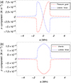 |
Fig. 5. Mechanical equilibrium along the magnetic field line for the reference model: a) longitudinal and b) vertical components of the forces. Only a region around the cold thread, the PCTR, and the beginning of the coronal part is displayed. |
Concerning the study of the energy balance, we computed the terms on the right-hand side of Eq. (32) using, again, the parameters of the reference model. Explicitly, these terms are the ambipolar heating rate, divergence of the heat flux due to thermal conduction, and the energy loss due to radiative cooling. Figure 6 compares the relevance of such terms along the magnetic field line in a zone encompassing the cool thread, the PCTR, and the beginning of the coronal region. The sign of each term indicates whether the term acts as an energy sink (negative) term or an energy source (positive) term. Obviously, radiative cooling is a sink term that extracts energy from the plasma. The radiative losses are most efficient within the PCTR, for a temperature of T ≈ 57 000 K, and their minimum (in absolute value) takes place in the cold prominence thread. The term due to thermal conduction follows a similar profile as that of radiative losses, especially in the PCTR and the coronal part, but with a positive sign. Finally, the ambipolar heating rate (Fig. 3i) is positive, as expected for a term that provides an energy input. However, this heating term is confined within the cool region where the plasma is partially ionized.
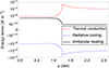 |
Fig. 6. Comparison of the energy terms in the heat-loss function (Eq. (32)) along the magnetic field line for the reference model. Only a region around the cold thread, the PCTR, and the beginning of the coronal part is displayed. Only half the domain with s ≥ 0 is displayed due to the symmetry of the profiles. In the coronal part, the ambipolar heating is set to a nonzero but negligible value for numerical stability reasons. |
Comparing the relevance of each term in the energy balance, we see that the radiative losses are entirely compensated by the thermal conduction in the PCTR and the coronal part, since the ambipolar heating is there absent. However, in the cool central region the important energy input provided by ambipolar heating partly compensates for the radiative losses, while the relative weight of the conduction term in the energy balance consequently decreases. These findings about the relevant role of the heating term in the cool thread are consistent with previous works, where either a prescribed uniform heating (Terradas et al. 2021) or a self-consistently computed nonuniform wave heating (Melis et al. 2023) were considered. An important difference with respect to those previous works is that the heating considered here is not arbitrarily imposed, as in Terradas et al. (2021), nor produced by external sources, as in Melis et al. (2023); instead, it is generated by the internal diffusion of the non-force-free magnetic field of the prominence itself.
The central values of the energy terms depend on T0 and p0. We computed additional models to study the dependence of the ambipolar heating at the center as a function of these two parameters and its importance compared with radiative losses. These results are displayed in Fig. 7 in the form of contour plots. Importantly, for every value of T0, there is a minimum value of p0 for which an equilibrium is achievabe. These critical values are represented with the dotted red line in Fig. 7 and are explored later in Sect. 3.3.
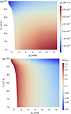 |
Fig. 7. Contour plots of the ambipolar heating at the center (upper panel) and the ratio between heating and cooling at the center (lower panel), as functions of T0 and p0. The color range in the upper panel is in lineal scale, whereas the lower panel is in logarithmic scale. |
Figure 7a represents the ambipolar heating at the center. The ambipolar heating is largest when the pressure is high and the temperature is low. This can be explained by the indirect relationship between the ambipolar heating and the mass density. According to Eq. (13), high pressures and low temperatures are associated with high densities. Then, according to Eq. (29), high densities are related to large values of dBx/dx; in turn, they give rise to large values of QA when Eq. (35) is taken into account. In more plain physical terms, the larger the density, the deeper the magnetic dip needs to be to support the plasma. Consequently, the larger the equilibrium current and so, the greater the heating produced by the dissipation of such a current. However, remarkably, the central heating is independent on both the horizontal magnetic field and the shear angle.
On the other hand, the ratio between the central values of the ambipolar heating and the radiative cooling can be seen in Fig. 7b for the same computations as before. For low and intermediate central pressures, the ambipolar heating can compensate for a significant fraction of radiative losses. In particular, for pressures lower than 6 mPa, the ambipolar heating can be as high as 90% of radiative losses, although for higher pressures the percentage decreases rapidly. For instance, for 10 mPa the ambipolar heating can only compensate for about 10% of radiative losses. We note that the ratio QA/Lrad. is almost independent of the central temperature, except for high temperatures approaching 10 000 K.
3.3. Parameter survey
Here, we investigate in more detail the effect of changing the free parameters of the model. We recall that these are the central pressure, p0, the horizontal magnetic field strength, B0, the shear angle, ϕ, and the central temperature, T0. We focus on analyzing the role of these parameters in the length of the cold thread, a. Realistic values of prominence thread lengths reported in observations are on the order of 2–30 Mm (see, e.g., Lin et al. 2005; Arregui et al. 2018). The parameter study was performed in the following way. Since there are four free parameters, we calculated the dependence of a with one specific parameter while keeping the other three parameters unchanged. This parameter survey is summarized in Fig. 8. Unless otherwise stated, the values of the unchanged parameters are same as those of the reference model of Sect. 3.1.
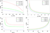 |
Fig. 8. Parameter survey of the thread length, a, in terms of the parameters: T0 (upper left), p0 (upper right), B0 (lower left), and ϕ (lower right). All the panels are in linear scale with the exception of the lower-right panel, which is in logarithmic scale. |
The effect of T0 is shown in Fig. 8a. Higher central temperatures produce shorter threads, which is related to the increasing efficiency of radiative losses when the temperature increases. This effect produces steeper temperature gradients in the conduction term and, consequently, shorter threads. This finding is consistent with previous works (see Terradas et al. 2021; Melis et al. 2023). Figure 8a contains three curves for three different values of p0, which show that, for the same temperature, the larger the central pressure, the shorter the cold thread. This result is explored in more detail in Fig. 8b, which displays a as a function of p0 for three different values of T0. Hence, Figs. 8a and b are reciprocal to each other. The influence of the central pressure on the thread length results from a complicated interplay between radiative losses and heating, as both ultimately depend on p0 through ρ, Bz, and the ionization degree. Findings from Terradas et al. (2021) and Melis et al. (2023) indicate that threads become shorter when the heating rate decreases in relation with the cooling rate. The result that larger pressures produce shorter threads can be explained by the fact that the heating rate decreases faster than the radiative losses at the core of the thread when p0 increases and T0 remains fixed, as previously shown in Fig. 7b. As already mentioned, the value of the central temperature determines a critical value of the central pressure below which an equilibrium is impossible. The larger T0, the smaller this critical p0. The existence of this critical pressure is related to the largest value of the plasma density that the magnetic field is able to support.
The influence of the strength of the horizontal magnetic field, B0, is shown in Fig. 8c. Stronger magnetic fields provide shorter threads, although the length saturates to a constant value once the magnetic field is strong enough. However, for weak magnetic fields the thread length increases asymptotically when B0 decreases, so that there is a critical value of the magnetic field strength for an equilibrium to exist, in a similar fashion as happens for the central pressure. As before, three different values of the central temperature have been considered, with higher temperatures providing shorter threads, thereby remaining consistent with the findings discussed before. Moreover, the central temperature also affects the critical value of the magnetic field strength, so that the critical B0 decreases when T0 increases. As an example, for T0 = 7000 K, the critical magnetic field strength is B0 ≈ 6.3 G; meanwhile for T0 = 9000 K, this value gets reduced to B0 ≈ 4 G. The combined effects of B0 and p0 are analyzed in more detail in Appendix B.
To conclude this parameter study, Fig. 8d shows the effect of the magnetic shear angle. The thread length increases for increasing shear angles in a more significant manner when the shear angle approaches 90°. For small magnetic shear, the thread length has unrealistically small values of less than 0.2 Mm. In this configuration, large magnetic shear is needed to obtain realistic values of the thread length of the order of 2 Mm or larger. We note that the equilibrium models are computed along the x-direction and then projected in the s-direction (i.e., the direction of the magnetic field) according the prescribed shear. Therefore, the total thread length depends on the shear angle through the relation a = ax/cos ϕ, where ax denotes the thread length measured along the x-direction, which is weakly modified when varying ϕ.
4. Discussion and caveats
In this paper, we explore the role of the heating produced by ambipolar diffusion in the energy balance of solar prominences, using an idealized 1D model. We considered a modified K-S configuration to construct models that satisfy both mechanical and energy equilibria, with the effect of ambipolar heating included in a consistent manner. We used a numerical method, based on that of Melis et al. (2023), where the balance of forces and the energy balance are solved iteratively until convergence to a self-consistent model is achieved.
The obtained models have a similar structure as those computed previously in Terradas et al. (2021) and Melis et al. (2023). A cool prominence region was found at the center, followed by a very thin PCTR, and an extended coronal region. The dense prominence plasma is supported against gravity by a shallow magnetic dip. In the cool prominence region, the plasma is partially ionized and ambipolar diffusion produces heating by dissipating currents associated with the non-force-free magnetic field. Additionally, ambipolar diffusion drives stationary flows associated with the gravitational drainage of neutrals.
A parameter survey was done to explore the variation of the length of the cold region. Cold regions with lengths compatible with those observed were obtained when realistic temperatures, pressures, and magnetic field strengths are considered, although the shear angle has an important effect. Only large values of the shear angle provide realistic cold thread lengths. In turn, there are critical values of p0, T0, and B0, for which computing an equilibrium configuration is no longer possible, and the length of the cold region increases asymptotically when those critical values are approached. Appendix B expands and complements the results of the parameter survey.
The force balance has been analyzed, showing that, essentially, magnetic tension compensates for gravity in the vertical direction, whereas magnetic pressure balances gas pressure in the horizontal direction. Regarding the energy balance, it has been demonstrated that the heating produced by ambipolar diffusion can partly compensate for the cooling by radiation. The ambipolar heating can balance almost entirely the radiative losses for very hot and tenuous threads. Considering more realistic values of temperature, pressure, and density, it is more conservative to state that ambipolar heating can compensate for, at least, 10% of radiative losses. We therefore conclude that the heating provided by the ambipolar diffusion of the prominence own magnetic field can play a non-negligible role in the energy balance of prominences.
The models explored here have some limitations that can be improved in the future. We used a 1D configuration, which obviate complexities that may appear in multidimensional models. An extension could be made by studying prominence threads in cylindrical geometry, which might include more ingredients such as the perpendicular component of thermal conduction. In this context, the study of thread widths in multidimensional models would be a natural extension of this work. Another limitation is that the models are stationary. However, prominences are dynamic objects that can suffer changes in relatively short periods of time. The models constructed here apply only to the global, large-scale quasi-equilibrium of prominences, ignoring the rich temporal evolution that is especially important at small scales. Another aspect we have not addressed is the stability of the constructed models. In this regard, the stability analysis of Bakhareva et al. (1992), including partial ionization effects, could be a starting point for future research. In this direction, studying the eigenmodes of the equilibrium models can help in determining their stability, as in Schmitt & Degenhardt (1995).
The results presented here can be qualitatively compared with those of recent time-dependent studies of prominence and coronal rain formation, allowing for potentially important effects that have not been included here to be identified. For instance, Jerčić et al. (2025) studied prominence formation in a 1D hydrodynamic setup using the two-fluid theory. Although their computed structures show similarities with our models in terms of temperature, density, and pressure profiles, the formation and evolution of shocks play a prominent role in their simulations. These dynamics cannot be captured by our stationary models. Additionally, the threads obtained in the simulations continuously accrete mass and increase their lengths beyond the limited lengths obtained from our equilibrium models; thus, reconciling the results of these different approaches requires further analysis. Similarly, Popescu Braileanu & Keppens (2025) used the two-fluid theory to study coronal rain formation in a 3D setup without gravity. Their results show that ionization and recombination processes play an important role in their simulations. However, ionization and recombination cannot be described with the single-fluid approach used here.
Although our focus here is set studying the influence of ambipolar heating and not on radiative losses, a potential limitation of this work is the approximate treatment of the cooling rates. We can roughly compare the radiative cooling rates obtained at the center of the reference model using the approximate cooling function (Eq. (43)) with those given in Gunár et al. (2025). To this end, we considered their results for a 1D vertical slab illuminated from its sides, using T = 8000 K and p = 0.05 dyn cm−2. To estimate the distance to the illuminated surface, we took into account that the length of the cold thread is 2.56 Mm, which means that the PCTR is located at a distance of 1.28 Mm from the center. Approximating the location of the PCTR as the location of the slab surface in the model of Gunár et al. (2025), we used L ≈ 1250 km (from their Table A.5). The tabulated cooling rate is ∼2 × 10⁻⁵ W m−3, which is about a factor of 10 greater than that computed from Eq. (43). Therefore, using the net radiative cooling rates of Gunár et al. (2025) could introduce some differences in the properties of the models discussed here. We plan to explore this in detail in a forthcoming work.
Acknowledgments
This publication is part of the R+D+i project PID2023-147708NB-I00, funded by MCIN/AEI/10.13039/501100011033 and by FEDER, EU. LM is supported by the predoctoral fellowship FPI_002_2022 funded by CAIB. We thank Prof. J. L. Ballester for reading a draft of this paper and for providing useful comments. We thank the anonymous referee for useful comments.
References
- Anzer, U. 2009, A&A, 497, 521 [NASA ADS] [CrossRef] [EDP Sciences] [Google Scholar]
- Anzer, U., & Heinzel, P. 1999, A&A, 349, 974 [NASA ADS] [Google Scholar]
- Anzer, U., & Heinzel, P. 2007, A&A, 467, 1285 [NASA ADS] [CrossRef] [EDP Sciences] [Google Scholar]
- Arregui, I., & Van Doorsselaere, T. 2024, in Magnetohydrodynamic Processes in Solar Plasmas, eds. A. K. Srivastava, M. Goossens, & I. Arregui, 415 [Google Scholar]
- Arregui, I., Oliver, R., & Ballester, J. L. 2018, Liv. Rev. Sol. Phys., 15, 3 [Google Scholar]
- Bakhareva, N. M., Zaitsev, V. V., & Khodachenko, M. L. 1992, Sol. Phys., 139, 299 [Google Scholar]
- Ballester, J. L., & Priest, E. R. 1987, Sol. Phys., 109, 335 [Google Scholar]
- Ballester, J. L., Alexeev, I., Collados, M., et al. 2018, Space Sci. Rev., 214, 58 [Google Scholar]
- Blokland, J. W. S., & Keppens, R. 2011, A&A, 532, A93 [NASA ADS] [CrossRef] [EDP Sciences] [Google Scholar]
- Braginskii, S. I. 1965, Rev. Plasma Phys., 1, 205 [Google Scholar]
- Brughmans, N., Jenkins, J. M., & Keppens, R. 2022, A&A, 668, A47 [NASA ADS] [CrossRef] [EDP Sciences] [Google Scholar]
- Chapman, S., & Cowling, T. G. 1970, The Mathematical Theory of Non-uniform Gases. An Account of the Kinetic Theory of Viscosity, Thermal Conduction and Diffusion in Gases (Cambridge: University Press) [Google Scholar]
- Degenhardt, U., & Deinzer, W. 1993, A&A, 278, 288 [NASA ADS] [Google Scholar]
- Donné, D., & Keppens, R. 2024, ApJ, 971, 90 [CrossRef] [Google Scholar]
- Draine, B. T. 1986, MNRAS, 220, 133 [NASA ADS] [Google Scholar]
- Gibson, S. E. 2018, Liv. Rev. Sol. Phys., 15, 7 [Google Scholar]
- Gilbert, H. 2015, in Solar Prominences, eds. J. C. Vial, & O. Engvold, Astrophys. Space Sci. Lib., 415, 157 [Google Scholar]
- Gilbert, H. R., Hansteen, V. H., & Holzer, T. E. 2002, ApJ, 577, 464 [NASA ADS] [CrossRef] [Google Scholar]
- Gilbert, H., Kilper, G., & Alexander, D. 2007, ApJ, 671, 978 [Google Scholar]
- Goodman, M. L. 2004, A&A, 416, 1159 [NASA ADS] [CrossRef] [EDP Sciences] [Google Scholar]
- Gunár, S., Heinzel, P., & Anzer, U. 2025, A&A, 699, A89 [NASA ADS] [CrossRef] [EDP Sciences] [Google Scholar]
- Hashimoto, Y., Ichimoto, K., & Huang, Y. 2023, PASJ, 75, 913 [Google Scholar]
- Heasley, J. N., & Mihalas, D. 1976, ApJ, 205, 273 [Google Scholar]
- Heinzel, P., & Anzer, U. 2001, A&A, 375, 1082 [NASA ADS] [CrossRef] [EDP Sciences] [Google Scholar]
- Heinzel, P., & Anzer, U. 2012, A&A, 539, A49 [NASA ADS] [CrossRef] [EDP Sciences] [Google Scholar]
- Heinzel, P., Anzer, U., & Gunár, S. 2010, Mem. Soc. Astron. It., 81, 654 [NASA ADS] [Google Scholar]
- Heinzel, P., Gunár, S., & Anzer, U. 2015, A&A, 579, A16 [NASA ADS] [CrossRef] [EDP Sciences] [Google Scholar]
- Heinzel, P., Gunár, S., & Jejčič, S. 2024, Phil. Trans. R. Soc. London Ser. A, 382, 20230221 [Google Scholar]
- Heinzel, P., Beck, D., Gunár, S., & Anzer, U. 2025, Sol. Phys., 300, 166 [Google Scholar]
- Hermans, J., & Keppens, R. 2021, A&A, 655, A36 [NASA ADS] [CrossRef] [EDP Sciences] [Google Scholar]
- Hillier, A., Shibata, K., & Isobe, H. 2010, PASJ, 62, 1231 [Google Scholar]
- Hood, A. W., & Anzer, U. 1990, Sol. Phys., 126, 117 [Google Scholar]
- Jerčić, V., Popescu Braileanu, B., & Keppens, R. 2025, ApJ, 986, 134 [Google Scholar]
- Karpen, J. T. 2015, in Solar Prominences, eds. J. C. Vial, & O. Engvold, Astrophys. Space Sci. Lib., 415, 237 [Google Scholar]
- Karpen, J. T., Antiochos, S. K., Hohensee, M., Klimchuk, J. A., & MacNeice, P. J. 2001, ApJ, 553, L85 [Google Scholar]
- Keppens, R., Zhou, Y., & Xia, C. 2025, Liv. Rev. Sol. Phys., 22, 4 [Google Scholar]
- Khomenko, E., & Collados, M. 2012, ApJ, 747, 87 [Google Scholar]
- Khomenko, E., Collados, M., Díaz, A., & Vitas, N. 2014, Phys. Plasmas, 21, 092901 [Google Scholar]
- Kippenhahn, R., & Schlüter, A. 1957, ZAp, 43, 36 [NASA ADS] [Google Scholar]
- Kuperus, M., & Raadu, M. A. 1974, A&A, 31, 189 [NASA ADS] [Google Scholar]
- Lin, Y. 2011, Space Sci. Rev., 158, 237 [Google Scholar]
- Lin, Y., Wiik, J. E., Engvold, O., Rouppe Van Der Voort, L., & Frank, Z. A. 2005, Sol. Phys., 227, 283 [Google Scholar]
- Low, B. C. 1975, ApJ, 198, 211 [Google Scholar]
- Low, B. C., & Petrie, G. J. D. 2005, ApJ, 626, 551 [Google Scholar]
- Low, B. C., & Wu, S. T. 1981, ApJ, 248, 335 [Google Scholar]
- Mandrini, C. H., Démoulin, P., & Klimchuk, J. A. 2000, ApJ, 530, 999 [NASA ADS] [CrossRef] [Google Scholar]
- Martin, S. F. 2015, in Solar Prominences, eds. J. C. Vial, & O. Engvold, Astrophys. Space Sci. Lib., 415, 205 [NASA ADS] [CrossRef] [Google Scholar]
- Martínez-Sykora, J., De Pontieu, B., Carlsson, M., et al. 2017, ApJ, 847, 36 [Google Scholar]
- Melis, L., Soler, R., & Ballester, J. L. 2021, A&A, 650, A45 [NASA ADS] [CrossRef] [EDP Sciences] [Google Scholar]
- Melis, L., Soler, R., & Terradas, J. 2023, A&A, 676, A25 [NASA ADS] [CrossRef] [EDP Sciences] [Google Scholar]
- Milne, A. M., Priest, E. R., & Roberts, B. 1979, ApJ, 232, 304 [Google Scholar]
- Oliver, R., Ballester, J. L., Hood, A. W., & Priest, E. R. 1992, ApJ, 400, 369 [Google Scholar]
- Oliver, R., Ballester, J. L., Hood, A. W., & Priest, E. R. 1993, ApJ, 409, 809 [Google Scholar]
- Parenti, S. 2014, Liv. Rev. Sol. Phys., 11, 1 [Google Scholar]
- Parenti, S., & Vial, J.-C. 2007, A&A, 469, 1109 [NASA ADS] [CrossRef] [EDP Sciences] [Google Scholar]
- Pécseli, H., & Engvold, O. 2000, Sol. Phys., 194, 73 [Google Scholar]
- Poland, A., & Anzer, U. 1971, Sol. Phys., 19, 401 [Google Scholar]
- Popescu Braileanu, B., & Keppens, R. 2025, A&A, 698, A189 [NASA ADS] [CrossRef] [EDP Sciences] [Google Scholar]
- Schmitt, D., & Degenhardt, U. 1995, Rev. Mod. Astron., 8, 61 [NASA ADS] [Google Scholar]
- Schure, K. M., Kosenko, D., Kaastra, J. S., Keppens, R., & Vink, J. 2009, A&A, 508, 751 [NASA ADS] [CrossRef] [EDP Sciences] [Google Scholar]
- Soler, R., Carbonell, M., & Ballester, J. L. 2015, ApJ, 810, 146 [Google Scholar]
- Soler, R., Terradas, J., Oliver, R., & Ballester, J. L. 2016, A&A, 592, A28 [NASA ADS] [CrossRef] [EDP Sciences] [Google Scholar]
- Spitzer, L. 1962, Physics of Fully Ionized Gases (New York: Interscience) [Google Scholar]
- Stepanov, A. V., Zaitsev, V. V., & Kupriyanova, E. G. 2024, Geomag. Aeronomy, 64, 1203 [Google Scholar]
- Terradas, J., Soler, R., Díaz, A. J., Oliver, R., & Ballester, J. L. 2013, ApJ, 778, 49 [Google Scholar]
- Terradas, J., Soler, R., Oliver, R., & Ballester, J. L. 2015, ApJ, 802, L28 [NASA ADS] [CrossRef] [Google Scholar]
- Terradas, J., Luna, M., Soler, R., et al. 2021, A&A, 653, A95 [NASA ADS] [CrossRef] [EDP Sciences] [Google Scholar]
- Tsinganos, K., & Surlantzis, G. 1992, A&A, 259, 585 [NASA ADS] [Google Scholar]
- Vial, J. C., & Engvold, O. 2015, in Solar Prominences, Astrophy. Space Sci. Lib., 415 [Google Scholar]
- Vigh, C. D., Gonzalez, R., & Rial, D. 2018, J. Phys. Conf. Ser., 1031, 012012 [Google Scholar]
- Vranjes, J., & Krstic, P. S. 2013, A&A, 554, A22 [NASA ADS] [CrossRef] [EDP Sciences] [Google Scholar]
- Wargnier, Q. M., Martínez-Sykora, J., Hansteen, V. H., & De Pontieu, B. 2022, ApJ, 933, 205 [NASA ADS] [CrossRef] [Google Scholar]
- Xia, C., Chen, P. F., Keppens, R., & van Marle, A. J. 2011, ApJ, 737, 27 [NASA ADS] [CrossRef] [Google Scholar]
- Zaqarashvili, T. V., Khodachenko, M. L., & Soler, R. 2013, A&A, 549, A113 [NASA ADS] [CrossRef] [EDP Sciences] [Google Scholar]
- Zhou, Y. 2025, Rev. Mod. Plasma Phys., 9, 32 [Google Scholar]
Updated values of the hydrogen ionization fraction are provided in Gunár et al. (2025). However, the differences with the previous results are small and have a negligible impact on our results.
We used an analytical fit of the numerically computed cooling curve available at https://erc-prominent.github.io/team/jorishermans/
Appendix A: Convergence of the solutions
Here, we briefly discuss the converge of the self-consistent method to compute equilibrium solutions. First, we explore the effect of the spatial resolution used in the numerical integration the energy balance equation to compute the temperature profile. Figure A.1 shows the evolution of the convergence parameter ε, as defined in Eq. (52), from iteration to iteration, for two different spatial resolutions and considering the same model parameters. For this set-up, only the case with high resolution correctly converges to a self-consistent model, as ε progressively decreases until the convergence threshold of ε = 10−7 is reached. We note that this threshold is arbitrary and is set after examining the evolution of many converging calculations. High resolution is crucial in regions where strong gradients are present. In this problem, the PCTR exhibits sharp variations in several physical quantities, which require a very fine resolution to be properly resolved. In the case with low resolution, the PCTR is not sufficiently resolved. Instead of converging to a self-consistent model, the iterative method enters a loop in which two different states alternate indefinitely. The convergence properties of the method can be compared with what was already discussed in Melis et al. (2023). In the previous paper, depending on the set of model parameters, the method either converged and produced cool thread models or became unstable, preventing the computation of physically consistent models.
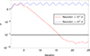 |
Fig. A.1. Comparison of the convergence of the parameter ε from iteration to iteration for two cases with different spatial resolutions. In both cases, the model parameters are T0 = 8000 K, p0 = 5 mPa, B0 = 10 G, and ϕ = 45°. The horizontal line denotes the convergence threshold of ε = 10−7. |
Another constraint that heavily affects the computation of physically acceptable models is the condition in Eq. (51), which corresponds to the requirement that the radiative losses at the thread center must be larger than the heating. In cases where this condition is not satisfied, it may still be possible to compute models that apparently converge according to the criterion based on the value of ε. However, those models are nonphysical. Figure A.2a shows a comparison of the evolution of ε in two situations: a case in which Eq. (51) is satisfied and another case in which it is not. Essentially, the difference between the two cases is the assumed value of the central pressure, p0. We find that both cases converge, with convergence being slightly faster in the low-pressure case than in the high-pressure case. Although both cases apparently converge, the computed temperature profiles differ significantly. This is shown in Fig. A.2b, where the final temperature profiles of both cases are compared. The high-pressure case satisfies Eq. (51) and the computed temperature profile has the expected shape. Conversely, Eq. (51) is not satisfied in the low-pressure computation, resulting in a temperature profile that displays an unexpected behavior. Instead of increasing toward coronal values when |s| increases, the temperature decreases and eventually reaches negative values, which is physically impossible. The reason for this behavior is that, when ambipolar heating exceeds radiative losses at the center, thermal conduction must become a negative term in the cool region to compensate the excess of heating. Consequently, the developed temperature gradient has the opposite sign (decreasing temperatures with increasing |s|) than in the physically acceptable solutions. Obviously, although the method has converged, these unacceptable solutions must be discarded.
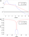 |
Fig. A.2. (a) Comparison of the convergence of the parameter ε from iteration to iteration for two cases with different central pressures. The horizontal line denotes the convergence threshold of ε = 10−7. (b) Converged temperature profiles for the same cases. In both cases, the model parameters are T0 = 8000 K, B0 = 10 G, and ϕ = 88°. |
Appendix B: Comparison with Milne et al. (1979)
Our research shares many similarities with the work of Milne et al. (1979), and also with the more recent paper by Vigh et al. (2018), although there are several important differences. Here, we discuss how these previous results can be compared with our findings.
Milne et al. (1979) assumed a fully ionized plasma, but we considered partial ionization, which incorporates two effects that have an important influence in the energy balance: ambipolar diffusion and the role of neutrals in the thermal conduction. Another relevant difference resides in the boundary conditions used to solve the energy balance equation. In our work, we imposed the temperature and the pressure at the center of the thread, in order to have a dense and cold region, and the energy equation is integrated from the center to the edge of the domain as in an initial-value problem. Conversely, Milne et al. (1979) set the temperature and the density at the edge of the domain to coronal values, while they imposed symmetry of both the vertical component of the magnetic field and the temperature at the center. Thus, in the case of Milne et al. (1979), the energy equation is integrated as a two-point, boundary-value problem, where the central temperature and pressure have to be determined rather than being fixed.
Because of the different numerical set-up, our results are not directly equivalent to those of Milne et al. (1979), although some comparisons can be made. Milne et al. (1979) discussed the existence of two types of solutions, the cool solutions and the hot solutions, whose appearance crucially depended on the plasma β = p0/(B02/2μ0), defined as the ratio between the gas and magnetic pressures, and the shear angle. Only in the case of the cool solutions, the central temperature is low enough to be consistent with prominence temperatures. Essentially, the temperature, pressure and density profiles in the cool solutions of Milne et al. (1979) are similar to the ones computed in the present paper, having a cold and dense region at the center and corona-like regions in the outermost part of the domain, as is seen in Figs. 10 and 11 of Milne et al. (1979). Hot solutions are not possible in our method, since we already imposed the temperature at the center to be that of cold prominences.
Milne et al. (1979) explained that there was a small range of β for which a cool equilibrium was computable. However, these allowed values of β are higher than the ones considered here. To further address this, Fig. B.1 displays a contour plot of the cold thread length as a function of both p0 and B0, for T0 = 8000 K and ϕ = 88°. The dashed purple lines denote several combinations of p0 and B0 that provide the same cold thread length (indicated next to every line). As discussed in Sect. 3.3, equilibrium models with high pressures have short cold threads, almost regardless of the magnetic field strength. Conversely, for low pressures, the computed thread lengths can reach values above 10 Mm for intense magnetic fields. Cold and dense threads with realistic lengths can only exist for sufficiently intense magnetic fields and relatively low pressures. This is explained by the fact that the weight of the dense plasma must be balanced by the upward magnetic force. If the magnetic field is too weak, the dense thread cannot be sustained. For every value of p0, there is a critical value of B0 above which an equilibrium is possible, and we see that the cold thread length increases abruptly when B0 approaches the critical value. The domain where an equilibrium can be reached is enclosed by a dotted red line in Fig. B.1, while no equilibrium is allowed in the white region. The dashed black lines included in Fig. B.1 indicate constant contours of β. Regions with relatively large β are related with short cold threads and with limited ranges of p0 and B0 where an equilibrium is possible. On the contrary, regions with small β are associated with longer cold threads and with wider ranges for p0 and B0. However, it is clear from the results of Fig. B.1 that the plasma β does not uniquely determine the length of the cold thread in our models. In fact, models with dramatically different cold thread lengths are possible along contours of constant β.
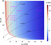 |
Fig. B.1. Contour plot of the cold thread length, a, as a function of p0 and B0. The dashed black lines represent contours of constant β, while the dashed purple lines represent contours of constant thread length. All the models are computed with T0 = 8,000 K and ϕ = 88°. |
The values of the cold thread length obtained in these computations are far larger than the ones obtained in Milne et al. (1979) for their standard model, but they obtained longer cold regions for larger values of the shear angle. This particular result agrees with our findings, although in the case of Milne et al. (1979) there was a maximum shear angle for an equilibrium to exist due to the constraints imposed by their boundary conditions. This maximum shear does not appear in our models. We recall that, in our models, the plasma ionization degree is also important and determines several physical parameters, such as the thermal conductivity and the ambipolar diffusion coefficient. The assumed value of T0 is very relevant concerning the plasma ionization degree. Therefore, the properties of our models and, in particular, the length of the cold thread, results from a complicated interplay between the four parameters: p0, B0, T0, and ϕ. Conversely, β and ϕ are the two crucial parameters that fully determine the properties of the models computed by Milne et al. (1979).
All Figures
|
Fig. 1. Ionization fractions of hydrogen and helium for p = 5 × 10⁻³ Pa as functions of the temperature, T. |
| In the text | |
|
Fig. 2. Visualization in 3D of the magnetic dip obtained for the reference model with T0 = 8000 K, p0 = 5 × 10⁻³ Pa, B0 = 10 G, and ϕ = 88°. The color gradient denotes the variation of the density along the magnetic field line. Note: the axes are not presented to scale. |
| In the text | |
|
Fig. 3. Equilibrium profiles along the magnetic field line for the reference model: a) temperature, b) mean atomic weight, c) z-component of the magnetic field, d) pressure, e) density, f) ambipolar diffusion coefficient, g) y-component of the velocity, h) z-component of the velocity, and i) ambipolar heating rate. Results for T0 = 8000 K, p0 = 5 × 10⁻³ Pa, B0 = 10 G and ϕ = 88°. The vertical dashed red lines mark the location of the cool and dense prominence thread of a length, a ≈ 2.56 Mm, as this the distance between the two lines. |
| In the text | |
|
Fig. 4. Close-up views of some quantities of the reference model around the cold thread and the PCTR: a) Mass fractions of protons (ionized hydrogen), singly ionized helium, and doubly ionized helium. b) Ambipolar diffusion coefficient. Only half the domain with s ≥ 0 is displayed due to the symmetry of the profiles. The discontinuous derivatives of the ambipolar diffusion coefficient are caused by the first-order interpolation used to implement the hydrogen ionization degree from the tabulated values in Heinzel et al. (2015). |
| In the text | |
|
Fig. 5. Mechanical equilibrium along the magnetic field line for the reference model: a) longitudinal and b) vertical components of the forces. Only a region around the cold thread, the PCTR, and the beginning of the coronal part is displayed. |
| In the text | |
|
Fig. 6. Comparison of the energy terms in the heat-loss function (Eq. (32)) along the magnetic field line for the reference model. Only a region around the cold thread, the PCTR, and the beginning of the coronal part is displayed. Only half the domain with s ≥ 0 is displayed due to the symmetry of the profiles. In the coronal part, the ambipolar heating is set to a nonzero but negligible value for numerical stability reasons. |
| In the text | |
|
Fig. 7. Contour plots of the ambipolar heating at the center (upper panel) and the ratio between heating and cooling at the center (lower panel), as functions of T0 and p0. The color range in the upper panel is in lineal scale, whereas the lower panel is in logarithmic scale. |
| In the text | |
|
Fig. 8. Parameter survey of the thread length, a, in terms of the parameters: T0 (upper left), p0 (upper right), B0 (lower left), and ϕ (lower right). All the panels are in linear scale with the exception of the lower-right panel, which is in logarithmic scale. |
| In the text | |
|
Fig. A.1. Comparison of the convergence of the parameter ε from iteration to iteration for two cases with different spatial resolutions. In both cases, the model parameters are T0 = 8000 K, p0 = 5 mPa, B0 = 10 G, and ϕ = 45°. The horizontal line denotes the convergence threshold of ε = 10−7. |
| In the text | |
|
Fig. A.2. (a) Comparison of the convergence of the parameter ε from iteration to iteration for two cases with different central pressures. The horizontal line denotes the convergence threshold of ε = 10−7. (b) Converged temperature profiles for the same cases. In both cases, the model parameters are T0 = 8000 K, B0 = 10 G, and ϕ = 88°. |
| In the text | |
|
Fig. B.1. Contour plot of the cold thread length, a, as a function of p0 and B0. The dashed black lines represent contours of constant β, while the dashed purple lines represent contours of constant thread length. All the models are computed with T0 = 8,000 K and ϕ = 88°. |
| In the text | |
Current usage metrics show cumulative count of Article Views (full-text article views including HTML views, PDF and ePub downloads, according to the available data) and Abstracts Views on Vision4Press platform.
Data correspond to usage on the plateform after 2015. The current usage metrics is available 48-96 hours after online publication and is updated daily on week days.
Initial download of the metrics may take a while.