| Issue |
A&A
Volume 708, April 2026
|
|
|---|---|---|
| Article Number | L8 | |
| Number of page(s) | 8 | |
| Section | Letters to the Editor | |
| DOI | https://doi.org/10.1051/0004-6361/202659450 | |
| Published online | 31 March 2026 | |
Letter to the Editor
Calibrating the tip of the red giant branch and measuring Magellanic Cloud distances to ∼2% exclusively with Gaia
1
Institute of Physics, École Polytechnique Fédérale de Lausanne (EPFL), Observatoire de Sauverny, 1290, Versoix, Switzerland
2
Institut für Astrophysik und Geophysik, Georg-August-Universität Göttingen, 37077, Göttingen, Germany
★ Corresponding authors: This email address is being protected from spambots. You need JavaScript enabled to view it.
; This email address is being protected from spambots. You need JavaScript enabled to view it.
Received:
14
February
2026
Accepted:
15
March
2026
Abstract
We have calibrated the tip of the red giant branch (TRGB) using our recent catalogue of homogeneous globular cluster (GC) distances. The GC distances were determined via a global joint fit to optical period–Wesenheit relations of their member RR Lyrae stars and type-II Cepheids, anchored by trigonometric parallaxes; all data were taken from the ESA Gaia mission’s (early) third data release (GDR3). Using I-band measurements of 48 GCs from P. Stetson’s database, we determined MI,0 = −3.948+0.037−0.034 mag (1.6% in distance). Calibrating the TRGB using Gaia’s homogeneous, space-based RP photometry of 53 GCs, we found MRP,0 = −3.807+0.041−0.035 mag (1.8%). The stated uncertainties include statistical and systematic effects, including the correlated nature of the GC distances. The robustness of our calibrations was evaluated via tests against small-number statistics and analysis choices. Within the (small) uncertainties, no significant metallicity effect is detected in our sample of old, low-metallicity GCs. We measured ∼2% distances to the Large and Small Magellanic Clouds, 18.447+0.036−0.042 mag (48.9 ± 0.9 kpc) and 18.898+0.049−0.054 mag (60.2 ± 1.4 kpc), respectively, using a single photometric system: RP (spectro-)photometry from GDR3. Our new TRGB distances, whose absolute scale derives from Gaia parallaxes, are fully independent of the well-known detached eclipsing binary (DEB) distances and agree with them to within the uncertainties. Combining our new TRGB and existing DEB distances, we illustrate how additional constraints can be incorporated into the Local Distance Network and obtain H0 = 73.52 ± 0.80 km s−1 Mpc−1. Expected improvements thanks to the upcoming fourth Gaia data release are discussed.
Key words: stars: distances / stars: Population II / globular clusters: general / Magellanic Clouds
© The Authors 2026
 Open Access article, published by EDP Sciences, under the terms of the Creative Commons Attribution License (https://creativecommons.org/licenses/by/4.0), which permits unrestricted use, distribution, and reproduction in any medium, provided the original work is properly cited.
This article is published in open access under the Subscribe to Open model. This email address is being protected from spambots. You need JavaScript enabled to view it. to support open access publication.
1. Introduction
The tip of the red giant branch (TRGB) is an empirical feature in the colour-absolute magnitude diagrams (CaMDs) of old stellar populations, and it is well understood to originate from the helium flash in first-ascent red giant stars (Salaris et al. 2002). The TRGB provides a useful standard candle for distance determination (Lee et al. 1993) and for measuring the Hubble constant, H0 (Li & Beaton 2024). The TRGB is the most commonly used extragalactic stellar distance indicator (Anand et al. 2021), and it is calibrated using known distances, preferably ones determined using geometrical methods. Since the TRGB magnitude is measured as the inflection point of the red giant branch luminosity function (LF) rather than using individual stars, this calibration most frequently relies on stellar populations observed at a common distance (for an exception, see Li et al. 2023). In particular, the detached eclipsing binary (DEB) distances to the Large (LMC) and Small Magellanic Clouds (SMC; Pietrzyński et al. 2019; Graczyk et al. 2020) and the water megamaser distance to NGC 4258 (Reid et al. 2019) have thus far enabled the most accurate TRGB calibrations. Galactic globular clusters (GCs) have also frequently been used to calibrate the TRGB, notably since the publication of trigonometric parallaxes from the (early) third data release of the ESA Gaia mission (GDR3; Gaia Collaboration 2016, 2021, 2023b). In particular, the catalogue of literature GC distances compiled in Baumgardt & Vasiliev (2021) has frequently been adopted for this purpose, even though the reported distances average correlated measurements (e.g. multiple distances based on the same set of RR Lyrae stars) alongside standard mean errors. Here, we seek to improve upon the Galactic TRGB calibration by anchoring it to our recent catalogue of 93 GC distances measured from a joint fit to period–Wesenheit relations of a large number of RR Lyrae stars and type-II Cepheids anchored to GDR3 parallaxes of GCs (Lengen et al. 2026; Cruz Reyes et al. 2024).
The H0DN Collaboration (2026) recently presented a 1% H0 measurement based on the Local Distance Network (LDN), a novel and extensible system of equations that combines high-quality low-redshift distance constraints in a statistically rigorous manner. The LDN’s absolute scale is anchored by geometrically measured distances, including the LMC’s DEBs (optionally also the SMC’s), the NGC 4258 megamaser, and Gaia parallaxes of classical Cepheids as well as average parallaxes of open clusters that host Cepheids. Creating additional linkages to the absolute scale provided by Gaia parallaxes is crucial for further improvements to the LDN’s robustness and H0 precision. The second goal of the present work was therefore to connect the LDN with the absolute scale of the GC distances from Lengen et al. (2026) by measuring the distances to the LMC and SMC using TRGB measurements performed in a single photometric system unaffected by atmospheric effects. Gaia’s RP band is very well suited to this end, given that it provides very precise photometry near the TRGB both in Galactic GCs and the Magellanic Clouds (Anderson et al. 2024; Koblischke & Anderson 2024, henceforth A24 and KA24, respectively). These new distances can independently cross-check DEB distances and illustrate how to incorporate new constraints into the LDN.
2. Data and methodology
We adopted GC distances from our recent global fit (Lengen et al. 2026) to optical period–Wesenheit relations of 802 RRab and 345 RRc stars, as well as 21 type-II Cepheids residing in 93 GCs, which relied on mean magnitudes from Clementini et al. (2023) and Ripepi et al. (2023). This global solution is anchored by accurate average parallaxes of 37 GCs from Cruz Reyes et al. (2024) determined using trigonometric parallaxes from GDR3 in the optimal magnitude range, where residual parallax bias (Lindegren et al. 2021a) is negligible, and taking the error floor due to angular covariance into account.
The metallicities, [Fe/H], and colour excesses, E(B − V), of GCs were taken from Harris (2010). Extinctions towards GCs were calculated assuming AI = 2.213 E(B − V) and ARP = 2.237 E(B − V) for RV = 3.3. In the Magellanic Clouds, we adopted extinction-corrected apparent TRGB magnitudes in the GDR3 RP band from KA24, who used colour excesses, E(V − I), from the Skowron et al. (2021) red clump star reddening maps and ARP = 1.486 E(V − I) in the LMC (assuming RV = 3.3) and ARP = 1.320 E(V − I) in the SMC (assuming RV = 2.7). All extinction coefficients were computed for a typical star near the TRGB using pysynphot and assuming the Fitzpatrick (1999) reddening law, following Anderson (2022). Appendix A discusses the sensitivity of our approach to reddening uncertainties.
The TRGB magnitudes were determined in three photometric systems: GDR3 RP, Cousins I band (determined from photometric transformations of GDR3 data; see Appendix B.3), and ground-based I-band observations. To this end, we compiled GDR3 photometry of GC member stars (Vasiliev & Baumgardt 2021) in the GDR3 RP, BP, and G bands (Riello et al. 2021), as well as in the Cousins I band via a cross-match (2″ search radius) with the September 2025 version of the Stetson et al. (2019) database1. Since the TRGB is populated by the brightest objects in a GC, we followed P. Stetson’s advice and carefully considered possible issues due to non-linearity or saturation (see Appendix B). However, no significant problems were identified.
We constructed a joint de-reddened CaMD using the samples of stars and GCs that passed the data selection criteria explained in Appendix C and listed in Table C.1. From the CaMDs, we constructed smoothed LFs using a GLOESS kernel of width σs = 0.125 mag, sampled in bins of 0.004 mag (see Appendix D for robustness tests against a range of GLOESS smoothing parameters). We measured absolute TRGB magnitudes from the resulting LFs as the inflection point of an unweighted [–1,0,1] Sobel filter following A24, ensuring consistency with the LMC and SMC measurements and avoiding bias due to differing TRGB contrasts. Uncertainties were determined via bootstrap resampling and taking correlations among the GC distances into account. Appendix E presents further details and convergence tests.
3. A 1.6% TRGB calibration based on Galactic GCs
Figure 1 illustrates the I-band CaMD, which combines 48 GCs and Stetson’s photometry alongside the smoothed LF and Sobel filter response. Table 1 lists our results for all three bands, with central values corresponding to the median of the bootstrap samples and (asymmetric) uncertainties representing the 16 − 84 percentiles.
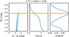 |
Fig. 1. CaMD, LF, and Sobel filter response for the combined GC sample based on the Stetson photometry. The purple line marks the median TRGB magnitude derived from the bootstrap analysis, and the orange contour indicates the 16–84th interquartile range. |
TRGB calibrations derived here.
The most precise result was obtained using Stetson’s GC photometry, which yielded the most stars near the TRGB. The resulting  mag (1.6% in distance) agrees with previous studies performed under similar conditions. Specifically, it agrees to within −0.022 mag (0.19σ) with the maximum-likelihood analysis of field stars by Li et al. (2023), who found
  mag. Soltis et al. (2021) previously reported MI, 0 = −3.97 ± 0.06 mag using GDR3 parallaxes of ω Cen. A larger difference is found with the unpublished study by Cerny et al. (2020), where 46 GCs were combined by matching horizontal branches; this yielded MI, 0 = −4.056 ± 0.02 (stat)±0.10 (sys). The difference of 0.108 mag with our determination does not exceed the uncertainty reported by Cerny et al. Their study was conducted as part of the Carnegie-Chicago Hubble Project (CCHP; Freedman et al. 2019), and we caution that part of the difference (∼0.06 mag) is readily explained by the weighting of Sobel filter response curves applied in the CCHP analysis. Such weighting results in brighter TRGB measurements, particularly in the case of the high contrast that is present in GCs (see Appendix B in A24).
Gaia photometry yielded similarly accurate I-band (by transformation; see Appendix B.3) and RP calibrations using five additional GC distances (53 instead of 48) and ∼40% fewer stars near the TRGB due to differences in the selection criteria. We note the near-perfect agreement between the transformed and native I-band calibrations.
We investigated the dependence of TRGB measurements on small-number statistics using (Stetson) I-band LFs and the metric N[ − 4, −3]*, the number of stars with MI0 ∈ [ − 4, −3], i.e. roughly one magnitude below the TRGB. Based on simulations, Madore & Freedman (1995) had argued that N[ − 4, −3]* > 100 was required for a reliable measurement; Madore et al. (2009) increased this to N[ − 4, −3]* > 400. Bellazzini et al. (2004) pointed out this issue for GCs, and Savino et al. (2022, see their Fig. 10) illustrated this effect by comparing TRGB and RR Lyrae distances to Andromeda’s satellites. To measure this effect in our GC sample, we randomly removed stars from the CaMD and repeated the TRGB measurements for 11 samples with N[ − 4, −3]* ∈ [100, 1086]. Figure 2 illustrates the deviations from the baseline and indicates that low statistics bias the measurement. Both the TRGB uncertainty and the bias behave asymptotically, nearing the baseline solutions for N[ − 4, −3]* ≳ 400, where the bias is of the order of 2 mmag of the baseline and the error approximately doubles. We stress that our approach combines information from many GCs and thus does not address the complex effect of how LFs are sampled in specific GCs (as discussed in Bellazzini et al. 2004).
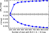 |
Fig. 2. Stability of the TRGB measurement under random star removal. Top: Median TRGB value as a function of sample size. The median decreases as the number of stars is reduced. Bottom: Corresponding evolution of the TRGB uncertainty. |
We investigated the effect of metallicity on the TRGB calibration by grouping GCs according to [Fe/H]. Since the GCs contain different numbers of stars, we devised an automatic binning procedure that minimized N[ − 4, −3]* in the largest bin. No significant trends were identified for Nbins ∈ [2, 4]. Using Nbins = 2, we found  for [Fe/H]= − 1.91 and
  for [Fe/H]= − 1.31, which are fully compatible with each other. Finer binning resulted in ever increasing uncertainties and remained uninformative. Our result is thus generally consistent with the expectation that old, low-metallicity populations ([Fe/H] < −1) exhibit no significant metallicity dependence in the I band (Salaris et al. 2002). Metallicity calibrations from the literature suggest a brighter TRGB at lower metallicities, albeit with significant scatter between calibrations. Specifically, the widely adopted Rizzi et al. (2007) calibration predicts a −0.017 mag difference based on the (V − I)0 difference of 0.079 mag. Larger corrections of −0.075 mag and −0.056 would be implied by the 0.6 dex [Fe/H] difference according to recent calibrations by Shao et al. (2025) and Yang et al. (2026), respectively, which rely on individual GCs. However, such calibrations are dominated by a few high-metallicity GCs, differ in their mathematical form (exponential or polynomials), and can be affected by the aforementioned stochastic issues.
While a TRGB metallicity dependence thus cannot be ruled out, we conclude that (a) this effect cannot be precisely constrained using this collection of GCs due to the generally low metallicity range and that (b) our calibration benefits from insensitivity to the stochastic sampling effects that impact analyses of individual GCs.
4. Magellanic Cloud distances to 2%
The distances to the Magellanic Clouds play crucial roles in the calibration of various standard candles and the extragalactic distance scale. The most commonly adopted distances to both galaxies, μLMC = 18.477 ± 0.004 (stat)±0.026 (sys) mag (1.1% in distance) in the LMC and μSMC = 18.977 ± 0.016 (stat)±0.028 (sys) mag (1.5% in distance) in the SMC, were determined geometrically using DEB systems composed of helium-burning giants (Pietrzyński et al. 2019; Graczyk et al. 2020). These distances were also used in the LDN to measure H0 (H0DN Collaboration 2026). Measuring both distances independently of the DEBs and with competitive accuracy thus provides crucial cross-checks.
Our 1.8% TRGB calibration based on Gaia’s RP observations provides such an opportunity: it benefits from a single space-based photometric system and an absolute scale provided by trigonometric parallaxes, and even takes the correlated nature of the GC distances into account. We thus determined  mag (1.8% in distance) and
  mag (2.4% in distance) using our value for MRP, 0 and the apparent magnitudes for the small-amplitude red giant (SARG) samples from Table 3 in KA24. We adopted SARG-based LMC TRGB measurements because (a) all stars near the TRGB are SARGs (A24), (b) the variability selection filters out contaminants similar to the astrometric membership in GCs, and (c) the SARG LFs in the LMC and SMC are inherently less sensitive to smoothing bias than the Allstars samples, similar to the combined LF constructed from the GCs (see Appendix D, notably Fig. D.1). Nevertheless, we stress that differences between the SARG and Allstars TRGB magnitudes in the LMC and SMC are negligible: 5 mmag and 1 mmag, respectively. For the LMC, our distance agrees to within < 0.7σ, or
  mag, with the DEB result. Analogously for the SMC, we find agreement within ∼1.3σ, or
  mag, with the DEB distance. The slightly worse agreement arises because the SMC-LMC TRGB magnitude difference of 0.450 mag (0.446 mag in the I band) is slightly smaller than the 0.500 mag difference among the DEB distances (see Sect. 3.2 in KA24).
Applying the colour-based metallicity corrections from Rizzi et al. (2007) would slightly increase our distances. Although these calibrations were derived in the I band, we applied them here to the GaiaRP measurements. This is justified by the nearly identical effective wavelengths of the two bands, which differ by only 9 nm (Jordi et al. 2010), implying that metallicity effects should be essentially the same. Empirical support for this assumption comes from KA24, who found that RP and I yield nearly identical LMC–SMC distance differences; for the SARG subsample, the offset is only 0.005 mag. Using the mean de-reddened colour of the GC sample near the TRGB, (V − I)0, GC = 1.49, and the values for SARGs in the LMC and SMC yields colour differences of 0.31 mag and 0.06 mag, respectively. This would yield ![Mathematical equation: $ \Delta \mu_{\mathrm{DEB-TRGB,LMC}}^{\mathrm{Zcorr}} = \Delta \mu_{\mathrm{DEB-TRGB}} - 0.217\left[(V-I)_{0,\mathrm{LMC}}-(V-I)_{0,\mathrm{GC}}\right] = -0.037\, \mathrm{mag} $](/articles/aa/full_html/2026/04/aa59450-26/aa59450-26-eq17.gif) and
and  mag, respectively, which remain within the 1σ uncertainties.
The H0DN Collaboration (2026) recently presented the LDN, a new and extensible framework for determining H0 by combining a large collection of distance measurements in a statistically rigorous manner. To illustrate the LDN’s philosophy, we incorporated our TRGB distances into the baseline solution (LMC only) and variant V07 (baseline + SMC). We computed weighted averages of the independent TRGB and DEB distances and obtained H0 = 73.52 ± 0.80 km s−1 Mpc−1 and 73.29 ± 0.78 km s−1 Mpc−1 for the modified baseline and V07, respectively. As expected given the aforementioned agreement in distances, and our larger uncertainties, no significant change in H0 was found, and uncertainties improved only marginally. Nonetheless, such an approach increases the robustness of the LDN and ties it more strongly to the absolute scale provided by Gaia’s trigonometric parallaxes.
5. Conclusions
We have calibrated the TRGB using 48 and 53 GCs in the I band and Gaia’s RP system, achieving the most accurate Milky Way TRGB calibration to date. The absolute scale is provided by a purely Gaia-based joint solution to 802 RRab, 345 RRc, and 21 type-II Cepheids residing in Galactic GCs anchored to average GC parallaxes (Lengen et al. 2026). Our I-band calibration based on ground-based data from the Stetson database yields  mag (1.6% in distance), which is in full agreement with previous studies and has a lower uncertainty. Stated uncertainties include statistical and systematic effects, including the correlated nature of the underlying GC distances. Additional investigations into the stability of the measurements against low statistics, a possible dependence on the smoothing parameter, and reddening and metallicity effects have been presented. In particular, we find no significant metallicity dependence of the TRGB in our sample of Galactic GCs, although this result is limited by either a restricted [Fe/H] range or by TRGB measurement bias and increased uncertainties resulting from stochastic effects. Conversely, we have shown that colour-based metallicity corrections from the literature would not significantly change our results.
Our GaiaRP calibration yields  mag (1.8% in distance) and offers the opportunity of measuring TRGB distances to the LMC and SMC with a single space-based photometric system and based on an absolute scale anchored to geometric distances. Using consistently measured TRGB apparent magnitudes from KA24, we obtained
  mag (1.8% in distance) and
  mag (2.4% in distance) in the LMC and SMC, respectively. These distances are entirely independent of, yet fully compatible with, the high-accuracy geometric DEB distances (Pietrzyński et al. 2019; Graczyk et al. 2020). Incorporating the weighted average of the new TRGB and existing DEB distances into the LDN as an example of its use yields a slightly improved uncertainty on H0: 73.52 ± 0.80 km s−1 Mpc−1 for the updated LDN baseline.
The upcoming fourth Gaia data release (GDR4), currently scheduled for December 2026, will enable several improvements since GDR4 will feature improved astrometric solutions, photometric calibrations, and variable star classifications. We thus anticipate that GDR4 will help decrease uncertainties in our TRGB calibration. Unless GDR3 is subject to as yet unknown systematics, central values of key quantities are expected to remain within the uncertainties because GDR4 will incorporate the observations underlying GDR3.
Additionally, GDR4 will enable studies of SARGs in GCs in analogy with the Magellanic Clouds (A24). Crowding limited both the number of GCs and stars therein that could be used in the present work. Improving photometric measurements in crowded regions and at the bright end of the GCs would thus be particularly valuable. Further improvements are likely thanks to homogeneous and detailed abundance measurements in GCs and the Magellanic Clouds based on the 4-metre Multi-Object Spectroscopic Telescope (4MOST; de Jong et al. 2019; Cioni et al. 2019; Lucatello et al. 2023), and differential reddening maps (Pancino et al. 2024) may further improve CaMDs.
Acknowledgments
MC and RIA were funded by a Swiss National Science Foundation Eccellenza Professorial Fellowship (award PCEFP2_194638). This research has received support from the European Research Council (ERC) under the European Union’s Horizon 2020 research and innovation programme (Grant Agreement No. 947660). This work has made use of data from the European Space Agency (ESA) mission Gaia (https://www.cosmos.esa.int/gaia), processed by the Gaia Data Processing and Analysis Consortium (DPAC, https://www.cosmos.esa.int/web/gaia/dpac/consortium). Funding for the DPAC has been provided by national institutions, in particular the institutions participating in the Gaia Multilateral Agreement.
References
- Anand, G. S., Rizzi, L., Tully, R. B., et al. 2021, AJ, 162, 80 [CrossRef] [Google Scholar]
- Anderson, R. I. 2022, A&A, 658, A148 [NASA ADS] [CrossRef] [EDP Sciences] [Google Scholar]
- Anderson, R. I., Koblischke, N. W., & Eyer, L. 2024, ApJ, 963, L43 [NASA ADS] [CrossRef] [Google Scholar]
- Baumgardt, H., & Vasiliev, E. 2021, MNRAS, 505, 5957 [NASA ADS] [CrossRef] [Google Scholar]
- Bellazzini, M., Ferraro, F. R., Sollima, A., Pancino, E., & Origlia, L. 2004, A&A, 424, 199 [NASA ADS] [CrossRef] [EDP Sciences] [Google Scholar]
- Cerny, W., Freedman, W. L., Madore, B. F., et al. 2020, AAS, submitted [arXiv:2012.09701] [Google Scholar]
- Cioni, M. R. L., Storm, J., Bell, C. P. M., et al. 2019, The Messenger, 175, 54 [NASA ADS] [Google Scholar]
- Clementini, G., Ripepi, V., Garofalo, A., et al. 2023, A&A, 674, A18 [NASA ADS] [CrossRef] [EDP Sciences] [Google Scholar]
- Cruz Reyes, M., Anderson, R. I., Johansson, L., Netzel, H., & Medaric, Z. 2024, A&A, 684, A173 [NASA ADS] [CrossRef] [EDP Sciences] [Google Scholar]
- de Jong, R. S., Agertz, O., Berbel, A. A., et al. 2019, The Messenger, 175, 3 [NASA ADS] [Google Scholar]
- Fitzpatrick, E. L. 1999, PASP, 111, 63 [Google Scholar]
- Freedman, W. L., Madore, B. F., Hatt, D., et al. 2019, ApJ, 882, 34 [Google Scholar]
- Gaia Collaboration (Prusti, T., et al.) 2016, A&A, 595, A1 [NASA ADS] [CrossRef] [EDP Sciences] [Google Scholar]
- Gaia Collaboration (Brown, A. G. A., et al.) 2021, A&A, 649, A1 [NASA ADS] [CrossRef] [EDP Sciences] [Google Scholar]
- Gaia Collaboration (Montegriffo, P., et al.) 2023a, A&A, 674, A33 [CrossRef] [EDP Sciences] [Google Scholar]
- Gaia Collaboration (Vallenari, A., et al.) 2023b, A&A, 674, A1 [NASA ADS] [CrossRef] [EDP Sciences] [Google Scholar]
- Gordon, K. 2024, J. Open Source Software, 9, 7023 [Google Scholar]
- Graczyk, D., Pietrzyński, G., Thompson, I. B., et al. 2020, ApJ, 904, 13 [Google Scholar]
- H0DN Collaboration (Casertano, S., et al.) 2026, A&A, in press, https://doi.org/10.1051/0004-6361/202557993 [Google Scholar]
- Harris, W. E. 2010, ArXiv e-prints [arXiv:1012.3224] [Google Scholar]
- Jordi, C., Gebran, M., Carrasco, J. M., et al. 2010, A&A, 523, A48 [NASA ADS] [CrossRef] [EDP Sciences] [Google Scholar]
- Kharchenko, N. V., Piskunov, A. E., Schilbach, E., Röser, S., & Scholz, R.-D. 2013, A&A, 558, A53 [NASA ADS] [CrossRef] [EDP Sciences] [Google Scholar]
- Koblischke, N. W., & Anderson, R. I. 2024, ApJ, 974, 181 [Google Scholar]
- Lee, M. G., Freedman, W. L., & Madore, B. F. 1993, ApJ, 417, 553 [Google Scholar]
- Lengen, B., Anderson, R. I., Cruz Reyes, M., & Viviani, G. 2026, A&A, 706, A87 [NASA ADS] [CrossRef] [EDP Sciences] [Google Scholar]
- Li, S., & Beaton, R. L. 2024, ArXiv e-prints [arXiv:2403.17048] [Google Scholar]
- Li, S., Casertano, S., & Riess, A. G. 2023, ApJ, 950, 83 [NASA ADS] [CrossRef] [Google Scholar]
- Lindegren, L., Bastian, U., Biermann, M., et al. 2021a, A&A, 649, A4 [EDP Sciences] [Google Scholar]
- Lindegren, L., Klioner, S. A., Hernández, J., et al. 2021b, A&A, 649, A2 [EDP Sciences] [Google Scholar]
- Lucatello, S., Bragaglia, A., Vallenari, A., et al. 2023, The Messenger, 190, 13 [NASA ADS] [Google Scholar]
- Madore, B. F., & Freedman, W. L. 1995, AJ, 109, 1645 [NASA ADS] [CrossRef] [Google Scholar]
- Madore, B. F., Mager, V., & Freedman, W. L. 2009, ApJ, 690, 389 [Google Scholar]
- Maíz Apellániz, J., Pantaleoni González, M., & Barbá, R. H. 2021, A&A, 649, A13 [NASA ADS] [CrossRef] [EDP Sciences] [Google Scholar]
- O’Donnell, J. E. 1994, ApJ, 422, 158 [Google Scholar]
- Pancino, E., Zocchi, A., Rainer, M., et al. 2024, A&A, 686, A283 [NASA ADS] [CrossRef] [EDP Sciences] [Google Scholar]
- Pietrzyński, G., Graczyk, D., Gallenne, A., et al. 2019, Nature, 567, 200 [Google Scholar]
- Reid, M. J., Pesce, D. W., & Riess, A. G. 2019, ApJ, 886, L27 [Google Scholar]
- Riello, M., De Angeli, F., Evans, D. W., et al. 2021, A&A, 649, A3 [NASA ADS] [CrossRef] [EDP Sciences] [Google Scholar]
- Ripepi, V., Clementini, G., Molinaro, R., et al. 2023, A&A, 674, A17 [NASA ADS] [CrossRef] [EDP Sciences] [Google Scholar]
- Rizzi, L., Tully, R. B., Makarov, D., et al. 2007, ApJ, 661, 815 [Google Scholar]
- Salaris, M., Cassisi, S., & Weiss, A. 2002, PASP, 114, 375 [NASA ADS] [CrossRef] [Google Scholar]
- Savino, A., Weisz, D. R., Skillman, E. D., et al. 2022, ApJ, 938, 101 [NASA ADS] [CrossRef] [Google Scholar]
- Shao, Z., Wang, S., Jiang, B., et al. 2025, ApJ, 980, 218 [Google Scholar]
- Skowron, D. M., Skowron, J., Udalski, A., et al. 2021, ApJS, 252, 23 [Google Scholar]
- Soltis, J., Casertano, S., & Riess, A. G. 2021, ApJ, 908, L5 [Google Scholar]
- Stetson, P. B., Pancino, E., Zocchi, A., Sanna, N., & Monelli, M. 2019, MNRAS, 485, 3042 [Google Scholar]
- Udalski, A., Skowron, D. M., Skowron, J., et al. 2025, Acta Astron., 75, 1 [Google Scholar]
- Valcin, D., Jimenez, R., Seljak, U., & Verde, L. 2025, JCAP, 2025, 030 [Google Scholar]
- Vasiliev, E., & Baumgardt, H. 2021, MNRAS, 505, 5978 [NASA ADS] [CrossRef] [Google Scholar]
- Yang, Y., Shao, Z., Wang, X., & Zheng, X. 2026, Res. Astron. Astrophys., 26, 035018 [Google Scholar]
Appendix A: Sensitivity to reddening
Since the absolute calibration of the TRGB depends on the adopted reddening, we examine its sensitivity to the assumed E(B − V) and RV values, taking the Harris (2010) catalogue as our reference. The GC sample used to calibrate the absolute magnitude in the RP band has a mean E(B − V) = 0.16, with only four clusters exceeding E(B − V) = 0.4. This indicates that the calibration sample is not dominated by heavily reddened objects, and therefore the choice of reddening reference is unlikely to introduce significant systematic shifts. Nevertheless, to test the robustness of this choice, we considered alternative reddening compilations.
Valcin et al. (2025) presented E(B − V) values for 69 GCs. For the clusters common to both catalogues and included in our RP calibration (37 of 53), we find  , corresponding to the 50th, 16th, and 84th percentiles of the distribution. The median offset is comparable to the mean measurement uncertainty in E(B − V) of 0.014. We therefore find no evidence for a systematic offset between the two reddening scales. However, adopting the Valcin et al. (2025) catalogue would reduce the calibration sample by ∼30%. We also compared the E(B − V) reddening values of Harris (2010) with those listed by Kharchenko et al. (2013), who state that they adopted the former. Despite this, we find small but systematic cluster-to-cluster differences between the two sets of values. For the clusters included in our RP calibration, we find E(B − V)Kharchenko − E(B − V)Harris = 0.001, with a standard deviation of 0.002. This difference is negligible for the absolute calibration of the TRGB.
We then turned to the sensitivity of the calibration to the assumed extinction law. Individual RV measurements are available for only a subsample of clusters, so we adopt a single value of RV = 3.3 with the Fitzpatrick (1999) reddening law, which yields AI/E(V − I) values equivalent to the O’Donnell (1994) law with RV = 3.0; this equivalence was obtained using the python package dust_extinction2 (Gordon 2024) and otherwise following (Anderson 2022). This choice is supported by the subset of our calibration clusters that also appear in Valcin et al. (2025), whose analysis was performed using the O’Donnell (1994) reddening law; for those clusters, RV = 2.99 ± 0.25 with an average uncertainty of 0.66. Although adopting a uniform RV introduces an additional source of uncertainty, it is unlikely to produce a significant bias: the calibration sample spans many independent sight lines, so cluster-to-cluster variations in the extinction law are expected to average out statistically. To quantify the impact of this assumption, we repeated the calibration using three values of RRP, the reference value RRP = 2.237, and two additional values offset by ±0.1. Relative to the reference solution, the absolute magnitude becomes brighter by 0.006 mag for the higher RRP and fainter by 0.012 mag for the lower RRP. We did not include this into the final uncertainty budget, as there is no clear basis for assigning a preferred range to the RRP distribution. Nevertheless, even if included, they would have a minor effect, since the uncertainties are added in quadrature and this contribution is smaller than our current uncertainties (∼0.040 mag).
Appendix B: Photometry
Peter Stetson’s website notes that the photometry of the brightest objects in each field may be affected by saturation and cautioned that such measurements should not be used without external verification of their quality. This appendix addresses that concern and shows that saturation does not represent an issue for our analysis. This point is particularly relevant here, as the brightest stars are precisely those used to measure the TRGB.
We first estimated the absolute magnitude of each star using the parameters described in Sect. 2 and grouped stars from all clusters into bins of 0.1 mag. The results are shown in Fig. B.1, which illustrates how the reduced chi-square (χPSF) of the point-spread-function (PSF) fitting varies as a function of absolute magnitude in the I band. As shown, χPSF reaches its maximum for the brightest stars and has a value close to 3 near the TRGB. It is worth noting that this behavior is limited to the I-band photometry from Stetson and has no impact on the Gaia RP band.
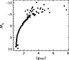 |
Fig. B.1. Absolute I-band magnitude, computed in 0.1 mag bins, as a function of the mean reduced χPSF. |
To assess the accuracy of these measurements, we employed two independent checks. The first uses Gaia synthetic photometry (Appendix B.1), and the second relies on photometric transformations derived from faint stars (Appendix B.2). Both tests indicate that the photometry is reliable.
B.1. Gaia synthetic photometry
To evaluate the quality of the Stetson photometry at the bright end, we computed Gaia I-band synthetic photometry (Gaia Collaboration 2023a) in the Johnson–Kron–Cousins system (‘JKC_Std’) for all GCs. The synthetic photometry was standardized using the Stetson et al. (2019) photometric standards, however, since these standards are fainter than the stars used to measure the TRGB, there is no a priori guarantee that the two photometric sets agree for bright sources.
We compared the sources for which both measurements are available. For this comparison, we use only sources brighter than the top 5% of the photometric standards in each field. We removed sources with |sharp|> 1 or ipd_frac_multi_peak > 10, clusters with high differential reddening, and clusters whose colour–magnitude diagrams appear contaminated by background stars. The results are shown in Fig. B.2. The mean difference of IGaia − IStetson is −0.001 ± 0.048 mag, where the uncertainty represents the standard deviation. Thus, we do not find evidence for a systematic bias in the Stetson photometry for bright sources. We decided not to use the synthetic photometry for the TRGB measurement, because only ∼12% of the stars in the Stetson sample have such measurements available.
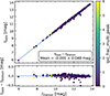 |
Fig. B.2. Comparison of Gaia synthetic photometry and Stetson photometry. No systematic bias is observed for stars brighter than the photometric standards, indicating that the Stetson photometry can be reliably used to measure the TRGB. |
B.2. Photometric transformations
A second check of the Stetson photometry for bright stars was obtained from photometric transformations calibrated using faint stars. To derive the I-band transformation, we used GaiaBP and RP photometry and excluded all stars brighter than the top 5% of the photometric standards in each field. We further applied the photometric quality cuts described in Appendix C. The transformation was modelled as Ipred ≡ RP + f(C), where f(C) is a third-order polynomial of the form  , with C = BP − RP. The propagated photometric uncertainty for each star was computed via standard error propagation as
 (B.1)
(B.1)
where f′(C) denotes the derivative of the polynomial with respect to C. The coefficients of the transformation appear in Table B.1.
Coefficients of the third-order polynomial fit.
The comparison between the photometry for sources brighter than the top 5% of the photometric standards (and therefore not used in the calibration of the transformations) is shown in Fig. B.3. The difference between the two measurements is statistically consistent with zero, and therefore there is no evidence of a photometric bias.
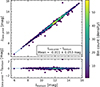 |
Fig. B.3. Comparison of the Stetson photometry of stars brighter than the top 5% of the standards and the photometry obtained by applying transformations calibrated using fainter stars. |
Appendix C: Data selection criteria
This appendix summarizes the full set of quality cuts applied to the photometric data, Gaia astrometry, and cluster-level parameters. These filters were designed to remove objects with poor photometry, unreliable Gaia measurements, or uncertain cluster properties.
We began with 93 clusters with measured distances (Lengen et al. 2026). The reddening cut, E(B − V) < 1, removed 5 clusters. The metallicity cut, [Fe/H]< − 0.9, excluded 7 additional clusters. Requiring more than 100 stars per cluster removed 9 more, and the condition nstars, fit > 2 excluded 14 clusters. In addition, 5 clusters were removed because their colour–magnitude diagrams exhibit strong differential reddening, or are significantly affected by contamination from foreground or background stars (NGC 6171, NGC 6266, NGC 6401, NGC 6626, and NGC 6715). After applying all criteria, the final sample contains 53 clusters, of which 48 have photometry in the I band. The adopted quality cuts are summarized in Table C.1, and the clusters used for the calibration in each band are listed in Table C.2.
Quality cuts.
Clusters used for the TRGB calibration in each band.
Appendix D: Sensitivity to smoothing
Previous studies (A24; Udalski et al. 2025) have shown that the choice of the GLOESS smoothing parameter can introduce systematic biases in the TRGB determination. To quantify the impact of this effect, we repeated the TRGB measurement in the IStetson band over a range of smoothing values, σs ∈ [0.10, 0.38] mag, in steps of 0.02 mag. The results are shown in Fig. D.1. Relative to the reference value adopted in Sect. 3, σs = 0.125, adopting σs = 0.15 shifts the mean TRGB to fainter magnitudes by 0.004 mag, whereas σs = 0.10 shifts it to brighter magnitudes by 0.005 mag. These offsets provide an estimate of the systematic uncertainty associated with the choice of the smoothing parameter.
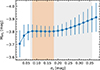 |
Fig. D.1. Variation in the mean and standard deviation of the TRGB magnitude as a function of the GLOESS smoothing parameter. The vertical grey lines indicate the range over which the absolute magnitude of the TRGB is insensitive to the smoothing value, according to A24 for their ‘SARGs’ sample. The orange shaded region was determined for the GC sample using the criterion |
Appendix E: Uncertainty propagation and convergence
The distances reported by Lengen et al. (2026) are mutually correlated. To propagate these correlations through the TRGB analysis, we used the Markov chain Monte Carlo (MCMC) samples presented in their Sect. 4.1.1, which represent the joint posterior distribution of the cluster distances. After discarding the burn-in phase and thinning the chains, we retained a set of P approximately independent MCMC realizations. Each realization corresponds to one instance of the full distance vector and therefore preserves the distance correlations. For each MCMC realization, we performed Q bootstrap re-samplings of the stars in each cluster to account for sampling variance. This procedure yielded a total of P × Q realizations. For each realization, we measured the TRGB absolute magnitude. The adopted TRGB value corresponds to the median of the resulting distribution, and the uncertainties are defined by the 16th and 84th percentiles. The total uncertainty budgets for both the TRGB absolute magnitude and the LMC and SMC distance moduli are listed in Table E.1.
Uncertainties included in TRGB calibration and LMC or SMC distances.
To assess the convergence of the sampling procedure, we analysed the sequence of TRGB measurements. We computed the cumulative mean of this sequence, μ, and defined the convergence point kconv as the first iteration at which the mean becomes stable. Specifically, we required that the last M values of μ remain within ϵ of μk, i.e.
 (E.1)
(E.1)
We first quantified how many MCMC samples are required to reach convergence. We found that NMCMC = 1, 500 samples are sufficient to achieve convergence at the ϵ = 0.001 mag level, adopting a stability window of M = 400 steps, and it is reached at kconv ≈ 666.
Having established convergence with the MCMC draws, we next evaluated the full sampling procedure, including the bootstrap re-samplings. After generating 10 bootstrap resamples for each MCMC realization and re-measuring the TRGB, we assessed convergence of the combined sequence of measurements. Since the realizations are naturally processed in order (i.e. the procedure is first applied to the first MCMC draw, then to the second, and so on), applying the convergence criterion to the ordered sequence could lead to convergence before incorporating information from the final realizations. To avoid this, we randomly shuffled the combined set of bootstrap measurements and evaluated convergence on the randomized sequence. We find that, on average, the combined sequence reached convergence at kconv ≈ 5618 at the ϵ = 0.001 mag level, using M = 4, 000. An example of a full run in the RP band is shown in Fig. E.1.
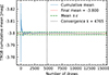 |
Fig. E.1. Convergence of the TRGB estimates in the RP band. The blue curve shows the cumulative mean TRGB absolute magnitude as a function of the number of sample draws. The red dashed line marks the final mean of the full sample. The dotted green lines indicate the final mean ±ϵ, with ϵ = 0.001 mag, and the black vertical line marks the convergence index kconv. As discussed in the text, the sample draws were randomly reordered; therefore, the exact shape of the curve may vary between permutations. |
All Tables
All Figures
|
Fig. 1. CaMD, LF, and Sobel filter response for the combined GC sample based on the Stetson photometry. The purple line marks the median TRGB magnitude derived from the bootstrap analysis, and the orange contour indicates the 16–84th interquartile range. |
| In the text | |
|
Fig. 2. Stability of the TRGB measurement under random star removal. Top: Median TRGB value as a function of sample size. The median decreases as the number of stars is reduced. Bottom: Corresponding evolution of the TRGB uncertainty. |
| In the text | |
|
Fig. B.1. Absolute I-band magnitude, computed in 0.1 mag bins, as a function of the mean reduced χPSF. |
| In the text | |
|
Fig. B.2. Comparison of Gaia synthetic photometry and Stetson photometry. No systematic bias is observed for stars brighter than the photometric standards, indicating that the Stetson photometry can be reliably used to measure the TRGB. |
| In the text | |
|
Fig. B.3. Comparison of the Stetson photometry of stars brighter than the top 5% of the standards and the photometry obtained by applying transformations calibrated using fainter stars. |
| In the text | |
|
Fig. D.1. Variation in the mean and standard deviation of the TRGB magnitude as a function of the GLOESS smoothing parameter. The vertical grey lines indicate the range over which the absolute magnitude of the TRGB is insensitive to the smoothing value, according to A24 for their ‘SARGs’ sample. The orange shaded region was determined for the GC sample using the criterion |
| In the text | |
|
Fig. E.1. Convergence of the TRGB estimates in the RP band. The blue curve shows the cumulative mean TRGB absolute magnitude as a function of the number of sample draws. The red dashed line marks the final mean of the full sample. The dotted green lines indicate the final mean ±ϵ, with ϵ = 0.001 mag, and the black vertical line marks the convergence index kconv. As discussed in the text, the sample draws were randomly reordered; therefore, the exact shape of the curve may vary between permutations. |
| In the text | |
Current usage metrics show cumulative count of Article Views (full-text article views including HTML views, PDF and ePub downloads, according to the available data) and Abstracts Views on Vision4Press platform.
Data correspond to usage on the plateform after 2015. The current usage metrics is available 48-96 hours after online publication and is updated daily on week days.
Initial download of the metrics may take a while.