| Issue |
A&A
Volume 709, May 2026
|
|
|---|---|---|
| Article Number | A69 | |
| Number of page(s) | 12 | |
| Section | Galactic structure, stellar clusters and populations | |
| DOI | https://doi.org/10.1051/0004-6361/202451201 | |
| Published online | 05 May 2026 | |
The GALAH survey: Searching for and characterizing halo substructures with the GALAH DR4 survey
1
Department of Astronomy, Stockholm University, AlbaNova University Center,
106 91
Stockholm,
Sweden
2
Research School of Astronomy and Astrophysics, The Australian National University,
Canberra
ACT2611,
Australia
3
Sydney Institute for Astronomy, School of Physics, A28, The University of Sydney,
Sydney,
NSW
2006,
Australia
4
Faculty of Mathematics and Physics, University of Ljubljana,
Jadranska 19,
1000
Ljubljana,
Slovenia
5
School of Mathematical and Physical Sciences, Macquarie University,
Balaclava Road,
Sydney,
NSW
2109,
Australia
6
ARC Centre of Excellence for All Sky Astrophysics in 3 Dimensions (ASTRO 3D),
Australia
7
School of Physics, University of New South Wales,
Sydney
NSW
2052,
Australia
8
Lund Observatory, Department of Geology,
Sölvegatan 12,
223 62
Lund,
Sweden
9
Astrophysics and Space Technologies Research Centre, Macquarie University,
Balaclava Road,
Sydney,
NSW
2109,
Australia
10
International Space Science Institute–Beijing,
1 Nanertiao, Zhongguancun, Hai Dian District,
Beijing
100190,
China
11
Space Telescope Science Institute,
3700 San Martin Drive,
Baltimore,
MD
21218,
USA
★ Corresponding author: This email address is being protected from spambots. You need JavaScript enabled to view it.
Received:
20
June
2024
Accepted:
9
February
2026
Abstract
Context. Recent studies have revealed that the Milky Way’s stellar halo is a composite of stellar populations of different origins, including multiple accretion events. To better understand how the Milky Way and other spiral galaxies were formed, it is necessary to thoroughly characterize the chemical and kinematic properties of these structures.
Aims. We search for kinematic structures of the stellar halo to find any substructures within them (when indeed present) and characterize the chemodynamical properties of the identified groups with the GALAH DR4 and Gaia surveys.
Methods. We applied wavelet transforms in the space defined by a square root of radial action (Jr) and azimuthal action (Lz) to search for kinematic overdensities. Then, we selected stars in the detected structures and investigated their elemental abundances to determine their origin. Additionally, we checked for any contamination from other stellar populations within the detected groups with the unsupervised machine learning algorithm t-Distributed Stochastic Neighbor Embedding (t-SNE), for which we performed chemical tagging in a high-dimensional parameter space using 15 elemental abundances as input.
Results. We recovered five kinematic structures in the action space with the wavelet transform. These groups are the Galactic disk, Splash, Gaia-Sausage-Enceladus (GSE), Thamnos1, and Thamnos2. We found that GSE has two peaks with the wavelet transform. One of these peaks is located at Jr ≃ 25 kpc km s−1 and is a result of contamination from disk stars. The other peak corresponds to the ‘cleanest’ GSE population and is located above Jr ≃ 40 kpc km s−1. We also detected three peaks in Thamnos. We linked two of them to Thamnos1, while the peak with the stars on the most retrograde orbits was linked to Thamnos2. The t-SNE algorithm confirmed these findings. We also analyzed individual elemental abundances of each group and found that Thamnos2 has a higher [α/Fe] ratio than the other groups and that iron-peak elements are more abundant in the Splash than in the halo groups, while the halo structures retain a higher r-process signature than the splashed disk.
Conclusions. A multiply peaked substructure we observe in action space in GSE and Thamnos suggests that the splashed disk extends beyond the borders of prograde orbits. Each of the four halo groups studied in this paper have unique chemodynamical properties that confirm their extra-galactic origin.
Key words: Galaxy: halo / Galaxy: kinematics and dynamics / Galaxy: structure
© The Authors 2026
 Open Access article, published by EDP Sciences, under the terms of the Creative Commons Attribution License (https://creativecommons.org/licenses/by/4.0), which permits unrestricted use, distribution, and reproduction in any medium, provided the original work is properly cited.
This article is published in open access under the Subscribe to Open model. This email address is being protected from spambots. You need JavaScript enabled to view it. to support open access publication.
1 Introduction
The formation and evolution process of large spiral galaxies is an active area of research in modern astronomy. Since the Milky Way is the only galaxy whose stars and structures can be studied in great detail, it is a benchmark for constraining models of galaxy formation. Therefore, performing highly detailed studies of the formation of the Milky Way is crucial to our understanding of spiral galaxies overall.
It is widely known that the Galaxy contains many kinematic structures and the nature and origins of these remain unresolved. A vast number of currently known structures have been found in the Galactic halo that have likely formed as a result of accretion events, where small galaxies merged with the Milky Way (e.g., Helmi et al. 2018; Belokurov et al. 2018; Koppelman et al. 2019; Myeong et al. 2019; Helmi 2020; Naidu et al. 2020; Ji et al. 2020; Deason & Belokurov 2024). Since accreted stars retain a similar chemical composition and motion to their progenitor (e.g. Freeman & Bland-Hawthorn 2002; Tolstoy et al. 2009), examining the chemodynamical properties of stars helps to separate accreted populations from those formed in situ. Thus, we need to have access to high-precision spectroscopic parameters and astrometric measurements for as many stars in the Galaxy as possible to discover new halo populations and characterize those already known.
Nowadays, large spectroscopic and astrometric surveys provide data for millions of stars and many millions more are expected in the near future. Current and future surveys include GAlactic Archaeology with HERMES (GALAH; De Silva et al. 2015), Apache Point Observatory Galactic Evolution Experiment (APOGEE; Holtzman et al. 2018), Large sky Area Multi-Object fibre Spectroscopic Telescope (LAMOST; Zhao et al. 2012), Hectochelle in the Halo at High resolution survey (H3; Conroy et al. 2019), and Gaia (Lindegren et al. 2016), as well as upcoming surveys such as 4-metre Multi-Object Spectroscopic Telescope (4MOST; de Jong et al. 2019) and the WHT Enhanced Area Velocity Explorer (WEAVE; Dalton et al. 2018, 2020), poised to deliver data on many more millions of stars. These and other surveys provide the necessary data to explore halo debris, which has led to several discoveries. For instance, Gaia-Sausage-Enceladus (GSE) (Belokurov et al. 2018; Helmi et al. 2018), which is linked to the last major merger that took place roughly 10 Gyr ago; the Sequoia accretion event (Myeong et al. 2019); Thamnos (Koppelman et al. 2018); and Heracles, the accreted population in the inner disk (Horta et al. 2021). It has also been shown that major merger events such as GSE can perturb the Galactic disk (Belokurov et al. 2020) and lead to the formation of kinematic structures such as the Splash. All these recent findings have raised interest in further investigating and characterizing the structures.
The discovery of these halo substructures has also raised the question of how we should select stars that come from the accreted progenitor only and avoid contamination from halo stars in other sources such as the Galactic disk. For instance, Feuillet et al. (2020) found that to get a “clean” subset of GSE stars, we should select stars with a square root of radial actions ![Mathematical equation: $\[\sqrt{J_{r}}\]$](/articles/aa/full_html/2026/05/aa51201-24/aa51201-24-eq3.png) > 30 kpc km s−1. The study of Buder et al. (2022) showed that, kinematically, GSE extends towards lower values of a square root of a radial action, with a mean value around
> 30 kpc km s−1. The study of Buder et al. (2022) showed that, kinematically, GSE extends towards lower values of a square root of a radial action, with a mean value around ![Mathematical equation: $\[\sqrt{J_{r}}\]$](/articles/aa/full_html/2026/05/aa51201-24/aa51201-24-eq4.png) ~ 26 kpc km s−1, and less than 30% of stars stay within the “clean” area. This means that purely kinematic criteria would remove a significant number of GSE stars with a lower square root of radial actions below 30 kpc km s−1. Subsequently, Feuillet et al. (2021) analyzed stars from the APOGEE and Gaia surveys and found that kinematically selected GSE and Sequoia populations contain a small number of in situ stars, which were identified on the basis of their elemental abundances.
~ 26 kpc km s−1, and less than 30% of stars stay within the “clean” area. This means that purely kinematic criteria would remove a significant number of GSE stars with a lower square root of radial actions below 30 kpc km s−1. Subsequently, Feuillet et al. (2021) analyzed stars from the APOGEE and Gaia surveys and found that kinematically selected GSE and Sequoia populations contain a small number of in situ stars, which were identified on the basis of their elemental abundances.
Accreted populations stand out from the disk stars not only dynamically, but also chemically, and most of them occupy partially overlapping regions in a multidimensional abundance space. For example, a study by Contursi et al. (2023) suggested that GSE has a higher Ce abundance than the Helmi streams, which is also an accreted population discovered by Helmi et al. (1999). It is known that GSE stars have lower [α/Fe] ratios compared to other halo stars, suggesting a different formation history (e.g., Haywood et al. 2018). Other structures, such as Thamnos and Heracles, exhibit a higher [α/Fe] than GSE (Horta et al. 2023). In addition, Matsuno et al. (2021) found that GSE is enhanced in r-process elements while being under-abundant in s-process elements. The mass estimate of the GSE progenitor by Lane et al. (2023) is ~1.45 × 10⁸M⊙ and is roughly 15–25% of the Milky Way’s stellar halo mass. The stellar mass of Thamnos is estimated to be ~5 × 10⁶M⊙ (Koppelman et al. 2019). The GSE accretion event occurred around eight to nine billion years ago, according to Helmi et al. (2018), while some recent studies (e.g., Feuillet et al. 2021) have suggested a slightly older age of 10–12 Gyr. At the time, tidal interactions between the disk and the GSE progenitor caused some of the old disk stars to gain vertical energy during the accretion event, creating a kinematically hot and physically thick disk with the same abundance pattern as the pre-interaction disk. According to Belokurov et al. (2020), these stars formed a kinematic structure known as the Splash.
Although so much progress has been made recently in characterizing these halo structures, many questions still need to be answered. One issue is related to whether there is any substructure within these newly discovered groups; especially in the GSE, as it is one of the largest known accreted groups to date. Answering this question would help us better understand the past and the structure of the GSE progenitor and our Galaxy. In this paper, we aim to search for kinematic structures of the stellar halo and any substructure within them, as well as to characterize their chemodynamical properties with the fourth data release from the GALAH survey (Buder et al. 2025).
We structure the paper in the following way. In Sect. 2, we describe the surveys used in this work and the construction of the stellar sample. In Sect. 3, we explain the methodology we used to search for structures in the stellar halo and we present the main results of this work. In Sect. 4, we check how many disk stars contaminate the halo structures we identified. In Sect. 5, we discuss the chemodynamical properties of each group. In Sect. 6, we describe the analysis of our sample with an alternative method. We summarize the paper in Sect. 7.
2 Data
To search for and characterize substructures in the stellar halo, we need a combination of kinematic parameters and elemental abundances for thousands of stars covering a wide range of Galactocentric radii and heights above and below the plane of the Galactic disk. In this work, we used elemental abundances and radial velocities from the GALAH survey (De Silva et al. 2015). GALAH is a high-resolution (R ~ 28 000) spectroscopic survey that provides stellar parameters and elemental abundances for stars in the Southern Hemisphere. We used the GALAH Data Release 4 (hereafter GALAH DR4; Buder et al. 2025), which contains almost a million stars. We combined spectroscopic data from GALAH DR4 with coordinates, parallaxes, and proper motions from the Gaia mission and used its latest Data Release 3 (hereafter Gaia DR3; Gaia Collaboration 2023). The distance estimates were taken from a complementary catalog by Bailer-Jones (2023). To select the most reliable elemental abundances and astrometric data for the analysis, we applied the following cuts:
flag_sp == 0;
snr_px_ccd3 > 30;
ruwe < 1.4;
survey_name = ‘galah_main’ or ‘galah_bright’ or ‘galah_faint’;
log g < 3.5;
4000 [K] < teff < 6500 [K].
These cuts produced the best-quality spectroscopic (cuts 1–2) and astrometric data (cut 3) and exclude open and globular clusters and other sub-surveys (cut 4). Applying cut 1 allowed us to select stars with no identified problems with the stellar parameter determination. With cut 2, we ensured that we would to get stars with a high signal-to-noise ratio (S/N) per pixel for CCD3. Cut 3 is a renormalized unit weight error for stars and is taken from the Gaia DR3 catalog. To avoid selection effects that might arise while mixing different types of stars across a wide range of Galactocentric radii, we limited our study to red giants only (cuts 5–6). Due to their long lifetimes and brightness, red giants are easily observed at great distances from the Sun, allowing us to explore different parts of the Galaxy, such as the stellar halo.
As a result, we ended up with a sample of 124 618 stars. Figure 1 shows the location of the selected stars in the Galactocentric cylindrical coordinate system. The Solar values of R = 8 kpc and Z = 20.8 pc, along with the solar motion corrections of U⊙ = 11.1 km s−1, V⊙ = 12.24 km s−1, and V⊙ = 7.25 km s−1 were taken from Bovy (2015) and Bennett & Bovy (2019). The majority of stars can be found in the direction opposite the NGP and are predominantly located towards the inner Galaxy (R ≲ 8 kpc). GALAH DR4 covers a broad range of Galactocentric radii and heights from the plane, allowing us to search for kinematic structures in the local stellar halo.
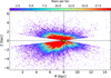 |
Fig. 1 Galactocentric distance, R, as a function of distance from the Galactic plane, Z, in the direction of the North Galactic Pole (NGP), Z = 90°, for 124 618 stars selected from GALAH DR4. Dashed lines show the Solar values R = 8 kpc and Z = 20.8 pc, while the yellow star shows the location of the Sun. The bin size is 0.05 × 0.05 kpc. |
3 Analysis and results
We searched for kinematic structures and examine a density distribution in the Lz − ![Mathematical equation: $\[\sqrt{J_{r}}\]$](/articles/aa/full_html/2026/05/aa51201-24/aa51201-24-eq5.png) space, as done in, for example, Trick et al. (2019). We applied the wavelet transform with the ‘a trous algorithm, which is an advanced statistical method previously described in Starck & Murtagh (2006). This method is commonly used to search for overdensities, including kinematic structures (e.g., Antoja et al. 2012; Kushniruk et al. 2017; Ramos et al. 2018). The wavelet transform has several significant advantages: no assumptions on the initial velocity distribution of stars are needed and the method allows us to detect a substructure in the sample (if present) at different decomposition levels proportional to the size of the structures we want to reveal.
space, as done in, for example, Trick et al. (2019). We applied the wavelet transform with the ‘a trous algorithm, which is an advanced statistical method previously described in Starck & Murtagh (2006). This method is commonly used to search for overdensities, including kinematic structures (e.g., Antoja et al. 2012; Kushniruk et al. 2017; Ramos et al. 2018). The wavelet transform has several significant advantages: no assumptions on the initial velocity distribution of stars are needed and the method allows us to detect a substructure in the sample (if present) at different decomposition levels proportional to the size of the structures we want to reveal.
We calculated orbital actions, such as the angular momenta, Lz, and the square root of radial actions, Jr, for all stars, assuming that the Galactic potential is axisymmetric. These quantities are fully conserved in axisymmetric systems and can thus be used to search for kinematic structures (Trick et al. 2019). The square root of Jr is proportional to the oscillation amplitude in the radial direction, representing the star’s epicyclic motion around its guiding radius. This relation is aptly illustrated in Figure 1 in Bland-Hawthorn & Tepper-García (2021). Therefore, using of ![Mathematical equation: $\[\sqrt{J_{r}}\]$](/articles/aa/full_html/2026/05/aa51201-24/aa51201-24-eq6.png) instead of Jr is beneficial for a dynamical characterization of the stellar populations. To calculate the actions, we used the galpy1 (Bovy 2015) package and the MWPotential2014 potential. The potential consists of the Navarro-Frenk-White halo, Miyamoto-Nagai disk, and a power-law bulge available through galpy.
instead of Jr is beneficial for a dynamical characterization of the stellar populations. To calculate the actions, we used the galpy1 (Bovy 2015) package and the MWPotential2014 potential. The potential consists of the Navarro-Frenk-White halo, Miyamoto-Nagai disk, and a power-law bulge available through galpy.
To perform the wavelet transform, we used the PyWavelets2 package (Lee et al. 2019). Wavelet coefficients are the main characteristic of the substructure and are proportional to the intensity of their detection. The input data come from a binned 2D distribution. After several tests, we found that the optimal number of bins which could provide a good balance between resolution and noise suppression for our sample was 512. The most suitable wavelet function was Symlet 2, as it is symmetrical and has a minimal oscillation. Among other wavelet functions, we found that Daubechies wavelet db 2 also recovered dynamical structures well in the data, but we chose Symlet 2 based on its highly symmetrical properties. When probing a range of decomposition steps, J, from 2 to 6, we set this parameter to 5 and 6, as this gives the best visual recovery of dynamical groups. The relation between decomposition levels, bin size, and sizes of the structures we searched for is SJ = 2JΔ (for more details, see Starck & Murtagh 2006). In our case, the bin size, Δ, for 512 bins is [![Mathematical equation: $\[\sqrt{J_{r}}\]$](/articles/aa/full_html/2026/05/aa51201-24/aa51201-24-eq7.png) , Lz] ≃ [0.2, 11.7] kpc km s−1. Thus, for a scale of J = 6, we searched for structures with sizes of [
, Lz] ≃ [0.2, 11.7] kpc km s−1. Thus, for a scale of J = 6, we searched for structures with sizes of [![Mathematical equation: $\[\sqrt{J_{r}}\]$](/articles/aa/full_html/2026/05/aa51201-24/aa51201-24-eq8.png) , Lz] ≃ [12.8, 748] kpc km s−1; similarly, for the scale J = 5, we recovered structures with sizes of [
, Lz] ≃ [12.8, 748] kpc km s−1; similarly, for the scale J = 5, we recovered structures with sizes of [![Mathematical equation: $\[\sqrt{J_{r}}\]$](/articles/aa/full_html/2026/05/aa51201-24/aa51201-24-eq9.png) , Lz] ≃ [6.4, 374] kpc km s−1.
, Lz] ≃ [6.4, 374] kpc km s−1.
Panel a of Figure 2 shows the initial 2D distribution of all 124 618 stars in the Lz − ![Mathematical equation: $\[\sqrt{J_{r}}\]$](/articles/aa/full_html/2026/05/aa51201-24/aa51201-24-eq10.png) space. The Galactic disk is a dominant part of our sample and is seen at
space. The Galactic disk is a dominant part of our sample and is seen at ![Mathematical equation: $\[\sqrt{J_{r}}\]$](/articles/aa/full_html/2026/05/aa51201-24/aa51201-24-eq11.png) < 20 kpc km s−1 and Lz > 1000 kpc km s−1. The halo part accounts for fewer stars, but it is clearly visible in the sample.
< 20 kpc km s−1 and Lz > 1000 kpc km s−1. The halo part accounts for fewer stars, but it is clearly visible in the sample.
As the next step, we generated 500 Monte Carlo Lz − ![Mathematical equation: $\[\sqrt{J_{r}}\]$](/articles/aa/full_html/2026/05/aa51201-24/aa51201-24-eq12.png) maps of the initial 2D distribution, shown in panel a of Figure 2, to which we applied the wavelet transform. This step is needed to check the significance of the detected overdensities. We calculated a covariance matrix between the parameters and found that most correlation coefficients are close to zero, indicating an insignificant dependence. Thus, we assume that a star’s radial velocity, coordinates, proper motions, and distances follow a Gaussian distribution, from which we drew values randomly and recalculated Lz −
maps of the initial 2D distribution, shown in panel a of Figure 2, to which we applied the wavelet transform. This step is needed to check the significance of the detected overdensities. We calculated a covariance matrix between the parameters and found that most correlation coefficients are close to zero, indicating an insignificant dependence. Thus, we assume that a star’s radial velocity, coordinates, proper motions, and distances follow a Gaussian distribution, from which we drew values randomly and recalculated Lz − ![Mathematical equation: $\[\sqrt{J_{r}}\]$](/articles/aa/full_html/2026/05/aa51201-24/aa51201-24-eq13.png) 500 times. The mean values and widths of the Gaussian distributions were defined by the measured values and their corresponding uncertainties were taken from the initial sample. Then, the wavelet transform was applied to every Monte Carlo-generated sample, with the central positions of all detected structures overplotted. Performing Monte Carlo simulations allowed us to estimate the sizes and uncertainties of the detected kinematic groups. We found that 500 Monte Carlo-generated samples are enough to converge the results.
500 times. The mean values and widths of the Gaussian distributions were defined by the measured values and their corresponding uncertainties were taken from the initial sample. Then, the wavelet transform was applied to every Monte Carlo-generated sample, with the central positions of all detected structures overplotted. Performing Monte Carlo simulations allowed us to estimate the sizes and uncertainties of the detected kinematic groups. We found that 500 Monte Carlo-generated samples are enough to converge the results.
The resulting wavelet transform maps for scales J = 5 and J = 6 are shown in panels b and c of Figure 2, respectively. Both plots show sums of the wavelet transform maps of all 500 Monte Carlo-generated samples. With the help of an image processing package for Python called scikit-image3 (van der Walt et al. 2014) and its peak detection algorithm, we found seven overdensities for scale J = 5 and two overdensities for scale J = 6, which are marked with white crosses. Based on a comparison of the results with the literature (e.g., Koppelman et al. 2018; Feuillet et al. 2020; Horta et al. 2021) the disk, Splash, GSE (two crosses above ![Mathematical equation: $\[\sqrt{J_{r}}\]$](/articles/aa/full_html/2026/05/aa51201-24/aa51201-24-eq14.png) > 20 kpc km s−1), Thamnos1, and Thamnos2 can be easily recognized based on their location on the Lz −
> 20 kpc km s−1), Thamnos1, and Thamnos2 can be easily recognized based on their location on the Lz − ![Mathematical equation: $\[\sqrt{J_{r}}\]$](/articles/aa/full_html/2026/05/aa51201-24/aa51201-24-eq15.png) map. We found that GSE consists of two peaks on a scale of J = 5, while Thamnos has three peaks that we can distil into Thamnos1 and Thamnos2 groups based on previous studies. Next, we drew ellipses around the crosses as shown on panel d of Figure 2 and selected stars inside the ellipses to further analyze the detected kinematic structures. The ellipses were drawn based on a visual inspection of the structures, with a comparison of the resulting wavelet space to existing findings in the literature. The centers of the ellipses, widths and heights, and the number of stars inside each group are given in Table 1. The biggest ellipse belongs to GSE, for which we combined two peaks based on the scale J = 5 as the structure is seen as a whole in the scale J = 6. We selected the most significant number of stars in the Splash population compared to the other groups. This reflects the dominance of the Solar neighborhood in the GALAH survey data.
map. We found that GSE consists of two peaks on a scale of J = 5, while Thamnos has three peaks that we can distil into Thamnos1 and Thamnos2 groups based on previous studies. Next, we drew ellipses around the crosses as shown on panel d of Figure 2 and selected stars inside the ellipses to further analyze the detected kinematic structures. The ellipses were drawn based on a visual inspection of the structures, with a comparison of the resulting wavelet space to existing findings in the literature. The centers of the ellipses, widths and heights, and the number of stars inside each group are given in Table 1. The biggest ellipse belongs to GSE, for which we combined two peaks based on the scale J = 5 as the structure is seen as a whole in the scale J = 6. We selected the most significant number of stars in the Splash population compared to the other groups. This reflects the dominance of the Solar neighborhood in the GALAH survey data.
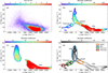 |
Fig. 2 Panel a: density map in Lz − |
![Mathematical equation: $\[\sqrt{J_{r}}\]$](/articles/aa/full_html/2026/05/aa51201-24/aa51201-24-eq16.png)
![Mathematical equation: $\[\sqrt{J_{r}}\]$](/articles/aa/full_html/2026/05/aa51201-24/aa51201-24-eq17.png)
![Mathematical equation: $\[\sqrt{J_{r}}\]$](/articles/aa/full_html/2026/05/aa51201-24/aa51201-24-eq18.png)
![Mathematical equation: $\[\sqrt{J_{r}}\]$](/articles/aa/full_html/2026/05/aa51201-24/aa51201-24-eq19.png)
Detected kinematic structures identified in this work.
4 Contamination of the structures from the disk and halo
In recent studies, such as those conducted by Feuillet et al. (2021), Horta et al. (2023), and Feltzing & Feuillet (2023), it was demonstrated that even though the kinematic and dynamical selection is efficient in identifying accreted halo populations, some in situ stars can still be included in the resulting sample. We checked fractions of stars that belong to the chemically defined disk and halo in the total sample. To split stars into the disk and halo populations, we followed the approach used in Buder et al. (2021) and studied the distribution of stars in the [Mg/Cu] versus [Na/Fe] space. [Mg/Cu] is a tracer of SNe II contributions from massive stars and SNIa of low-mass stars (Kobayashi et al. 2020). Similarly to [Mg/Fe], [Na/Fe] allows tracking differences between the in situ and accreted stars (e.g., Nissen & Schuster 2010).
We also selected stars for which there are no identified problems with abundance determination of a chemical element X by setting the flag flag_X_fe to zero. We applied this flag to each of the earlier-mentioned chemical elements to avoid inaccuracies in the analysis. The flags are given in the GALAH DR4 survey. Applying the flags to Mg, Cu, Na, and Fe abundances reduces the sample to 116 047 stars. Figure 3 shows the fractions of stars belonging to the disk population (below the dashed line) and the halo (above the dashed line). The dashed line was visually determined after examining the density distribution. Figure 4 shows the sample of 116 047 GALAH stars in gray and the different colors and shapes show stars in the Splash, GSE, Thamnos1, and Thamnos2 structures. Some stars in the disk population are found to fall into the part of the plot around [Na/Fe] ≃ −0.17, which is merely an artifact of the GALAH spectroscopic analysis pipeline. However, despite this, we do not exclude them from the study as most of these stars still belong to the disk population rather than the halo. Below, we discuss contamination fractions for each of the detected kinematic structures.
Splash: by its definition, the Splash ought to be composed of stars with disk-like chemistry that were brought to halo-like orbits by the last major merger event (see Belokurov et al. 2018). According to this definition, we found that ≈86% of stars in the group we found can be categorized as chemically belonging to the disk, while the remaining ≈14% exhibit chemical characteristics associated with the halo.
GSE: the GSE population originates from the last merger event and consists of accreted stars from the satellite Enceladus (Helmi et al. 2018). Thus, GSE stars are expected to be chemically distinct from the disk stars. Panel b of Figure 4 shows that ≈57% stars in the group we link to the GSE belong to the stellar halo, while the contamination from the disk is ≃43%.
Thamnos1: Thamnos1 is also believed to be a remnant of an accretion event and, thus, chemically differentiable from the disk (Koppelman et al. 2019). In the plot on panel c of Figure 4, we see that the contamination from the disk is ≃55%, and there is only ≃45% of halo stars.
Thamnos2: similarly to Thamnos1, Thamnos2 is expected to be clean from the disk stars. Panel d of Figure 4 shows that ≃88% of the stars belong to the halo and only one object is a disk star (≃12%).
Taking into account the definitions of the aforementioned kinematic structures and their contamination fractions, we decided to exclude chemically defined halo stars from the Splash and chemically defined disk stars from the remaining four groups. More details are given in Figure 4.
Figure 5 shows the orbital energy distribution as a function of angular momentum and the rotational velocity versus metallicity for the entire sample and the kinematic structures detected. The results we observe here are in agreement with other studies that investigated similar distributions, such as Koppelman et al. (2019) and Belokurov et al. (2018). The Splash is a connection between the Galactic disk stars and halo populations. The minor difference we have observed is that although stars in the GSE (Galactic substructure) population are close to Lz ≃ 0 kpc km s−1, they tend to follow slightly more retrograde orbits than prograde ones.
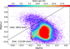 |
Fig. 3 Binned distributions of 116 047 stars selected from the GALAH DR4 in the [Mg/Cu] − [Na/Fe] plane. The bin size is 0.01 × 0.01. The dashed line shows the division of stars into the disk (below the line) and halo (above the line) stars. |
KDE metallicity peak values for the detected kinematic structures.
5 Chemodynamical characterization of the groups
Figure 6 shows normalized metallicity distributions and corresponding uncertainties for the detected kinematic structures. These distributions were derived using kernel density estimation (KDE) algorithms from the scikit-learn4 package (Pedregosa et al. 2011). Contamination of the halo and disk was removed for the Splash and the rest of the groups, respectively (see Sect. 4). Table 2 provides metallicity values, [Fe/H], where the normalized probability density has a maximum value and corresponding uncertainties, δ. All groups have wide metallicity distributions and distributions of Galactocentric radii. Thamnos1 and Thamnos2 appear to have multiple-peaked distributions. This could be due to potential substructure within the groups or remaining contamination of the structures by field stars. GSE is the structure that covers the broadest range of Galactocentric radii and extends to the outer Galaxy (R ≳ 8 kpc). The metallicity distribution of the GSE peaks at ≃−1.2 and is in agreement with other studies such as Naidu et al. (2020), who found a value of ≃−1.2, and Feuillet et al. (2021), who found a mean value of ≃−1.15. The peak of the metallicity distribution of Splash is ≃−0.6, which is in agreement with, for example, Belokurov et al. (2020) and Sanders et al. (2021). However, Thamnos1 and Thamnos2 have mean metallicities ≃−1.4 according to Bellazzini et al. (2023); whereas, in our study, we found the peak of the metallicity distribution at ≃−1.2 for Thamnos1 and ≃−1.3 for Thamnos2, although these differences are still within the errors.
Figure 7 shows the individual distributions of elemental abundances of all five kinematic structures, which are presented as box plots for 32 chemical elements. We included only stars for which individual elemental abundance flags, flag_X_fe = 0, to get the most precise data for the box plots. We note that the Mg, Fe, Cu, and Na abundances were used to identify populations, which means that we cannot draw purely independent conclusions based on these chemical elements.
Figure 8 shows a more detailed view of several elemental abundance spaces, such as [Mg/Fe], [Ba/Fe], and [Ba/Mg] as a function of metallicity. All of these chemical spaces provide details about the star formation history of the detected kinematic groups, as all of these chemical elements have different origins. The running means of the detected structures are shown as colored lines, and the corresponding errors are shown as shaded regions. These shaded regions represent the standard error of the mean within each running window, calculated from the individual abundance uncertainties of the stars in that window. The total sample is shown in the background as gray dots for comparison. The window size for the running means was estimated based on the number of stars in each kinematic group and ranges from 5 to 50. The step size was adopted as half the window size. Since Thamnos2 has very few stars for the running means, we show them as a scatter plot.
The uneven running mean of Thamnos1 results from several factors. Firstly, Thamnos1 has fewer identified stars compared to GSE and Splash. Secondly, the spike in Thamnos1 in panels b and c of Fig. 8 is likely due to contamination in the sample. This further emphasized the importance of combining both dynamical and chemical parameters to obtain the purest sample possible. Below, we discuss the elemental abundance patterns of each of the detected kinematic structures based on Figures 7 and 8.
The abundance of α-elements such as C, O, Ca, Mg, Al, Si, and Ti are slightly higher in the halo structures. This is especially noticeable for Thamnos2, whose oxygen abundance is higher than that of the rest of the groups. This result is in agreement with Horta et al. (2023), who showed that Thamnos shows a higher [α/Fe] ratio than the other halo substructures.
Iron-peak elements, including Co, Cr, Fe, Mn, Ni, Sc, and V, show different behaviours. Co, Fe, Ni, Sc, and V are more abundant in Splash than in the halo structures. The distributions of Cr and Mn are monotonic and do not vary between the groups. Sanders et al. (2021) and later Nissen et al. (2024) studied iron-peak abundances in the accreted halo populations and found low abundances of [Ni/Fe]. We observe a minor underabundance of [Ni/Fe] in the accreted populations compared to Splash.
Typical s-process (slow neutron-capture process) elements such as Ba, Ce, La, Mo, Nd, Rb, Sr, Y, and Zr are abundant in the accreted populations. The exception is Rb, whose abundance is lower for GSE than the rest of the structures, and Sr, for which very few stars in the structures have measurements. Thus, there are insufficient statistics for a proper analysis. However, Matsuno et al. (2021) found a contribution of r-process elements dominates over s-process. This is in agreement with our results for other s-process elements in GSE, such as Ba (see Fig. 8). The abundance of Ce, an s-process element, is much higher in GSE than in Splash, which contradicts the idea of low s-process abundances in GSE. Contursi et al. (2023) found that Thamnos and GSE have similar Ce abundance, while our box plots show that GSE and Thamnos2 have a slightly lower median than Thamnos1.
GALAH DR4 provides abundances of the following r-process (rapid neutron-capture process) elements: Eu, Nd, and Sm. Eu is not used here due to its current unreliability in DR4. GSE tends to have a higher abundance of r-process elements than other structures. This result is also in agreement with previous findings on GSE (Matsuno et al. 2021).
The abundance of Cu, Ru, and Zn, elements produced by explosive and non-explosive nucleosynthesis, show different patterns. Copper is more abundant in Splash than the halo groups and is likely because we chemically defined disk and halo groups using Cu abundance (see Sect. 4). The abundance of Ruthenium is higher for GSE than Splash and Thamnos1. Finally, Zn is slightly more abundant in Thamnos1 and Thamnos2.
Abundances of K and Na, elements primarily produced through nucleosynthesis in stars. Both elements are slightly more abundant in the halo structures, although we used the Na abundance to divide samples into the chemically defined disk and halo.
Halo structures are more abundant in Li compared to Splash. The abundance of lithium in GSE was studied, for example, by Molaro et al. (2020) and Simpson et al. (2021). It was shown that The A(Li) abundances versus [Fe/H] in the GSE population behave similarly to in situ stars, especially at low metallicities.
The [Mg/Fe]–[Fe/H] space (see panel a in Fig. 8) shows a negative slope for all groups, reflecting the overall decline of α-element abundances with increasing metallicity. The Splash occupies the thick disk region of the distribution, while GSE exhibits lower [Mg/Fe] values than both the Splash and Thamnos1. Thamnos1 follows a trend very similar to the Splash, indicating a later α-knee and more efficient chemical enrichment. We note that possible contamination in the Thamnos1 selection may blur this trend. This behaviour is consistent with Thamnos1 having experienced more rapid star formation than GSE and is in agreement with, for example, Horta et al. (2021), who explored the chemical properties of kinematic substructures using the APOGEE survey.
Thamnos1 and GSE show a similar behavior in the [Ba/Fe]–[Fe/H] and [Ba/Mg]–[Fe/H] spaces (see panels b, and c in Fig. 8), with both displaying increasing trends with metallicity. The slope is steeper for Thamnos1 than for GSE, consistent with more rapid star formation and a stronger delayed contribution from AGB stars. The Splash exhibits a shallower slope, more similar to GSE, indicating that Thamnos1 may have undergone a chemical evolution different from both the Milky Way and GSE. We note that contamination and small number statistics may affect the precise slopes, but the overall trend is consistent with faster enrichment for Thamnos1.
Overall, the accreted halo populations are chemically different from the disk stars. We also observed differences in elemental abundances among the dynamical populations, confirming that these groups have an extragalactic origin. While the conclusion is indeed influenced by our chemical grouping, carrying out the chemical, dynamical, and kinematic selections together is essential to neatly selecting stars that belong to the accreted groups.
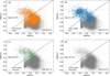 |
Fig. 4 Scatter plot of all 116 047 stars selected from GALAH DR4 in the [Mg/Cu] − [Na/Fe] plane is shown in gray. The markers of different colors show stars in the following kinematic structures: Splash (Panel a, orange circles), GSE (Panel b, blue circles), Thamnos1 (Panel c, green circles), and Thamnos2 (Panel d, red circles). The dashed line is the same as on panel a and divides the stars into the disk and halo sub-samples. Percentages of the halo and disk stars in the kinematic structures are provided in each plot. |
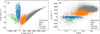 |
Fig. 5 Panel a: orbital energy plotted as a function of the angular momentum. Gray dots show a scatter plot of the total sample, while the other colors and symbols correspond to the kinematic structures detected in the legend. Chemically defined halo stars were excluded from the Splash and chemically defined disk stars were excluded from the rest of the groups. Panel b: similar to the plot in panel a, but showing the rotational velocity as a function of metallicity. |
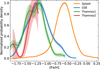 |
Fig. 6 Normalized probability density metallicity [Fe/H] with uncertainty bands for kinematic groups listed in the legend. The chemically defined halo stars were excluded from the Splash and chemicall -defined disk stars were excluded from the rest of the groups. The plot is generated using a kernel density estimation (KDE) with a bandwidth of 0.075 and a Gaussian kernel. The shaded regions around each curve represent corresponding uncertainties, which are standard deviations of 100 bootstrap samples. |
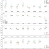 |
Fig. 7 Panels a–d: individual distributions of elemental abundances for the Splash (orange box), GSE (blue box), Thamnos1 (green box), and Thamnos2 (red box), which are depicted using box plots. The analysis covers 32 chemical elements, X, related to iron, [X/Fe], and iron abundance, which is related to hydrogen, [Fe/H]. Each box plot adheres to standard conventions, with the first and third quartiles defining the box body, “whiskers” extending to minimum and maximum values, and the median shown as a black line inside each box. |
6 Chemodynamical tagging of the accreted structures with t-SNE
Given that both dynamics and chemistry are essential for selecting halo substructures, we also investigated a method of selecting the halo substructures based solely on chemistry, to complement the dynamical selection using wavelets. To accomplish this, we used the algorithm t-distributed stochastic neighbor embedding (t-SNE), which implements dimensionality reduction based on nonlinear manifold learning (Hinton & Roweis 2002; van der Maaten & Hinton 2008). Kos et al. (2018) showed the efficiency of this algorithm for identifying ejected stars from star clusters using chemical tagging with GALAH data, identifying two ejected stars several degrees from the main body of the Pleiades open cluster. A follow-up study by Youakim et al. (2023) combined both chemistry and kinematics from GALAH data, using 20 parameters as input into t-SNE and finding several tidally stripped stars from Omega Centauri, thereby constraining the cluster’s initial mass and evolution time in the Galaxy. In another recent study conducted by Ortigoza-Urdaneta et al. (2023), the t-SNE algorithm was used to investigate chemical structures in a sample of 1742 red giants with rotational velocity Vϕ < 100 km s−1. The sample was selected from the APOGEE DR17 (Abdurro’uf et al. 2022) and Gaia surveys. The input parameters of the t-SNE analysis included elemental abundances of 10 chemical elements. As a result of their study, they identified the GSE and Splash populations, as well as a few new structures. Taken together, these results demonstrate that the t-SNE algorithm is a helpful tool for grouping stars based on their chemical properties.
As input for the t-SNE algorithm in this study, we included measured abundances of 15 chemical elements: [Fe/H], [O/Fe], [Na/Fe], [Mg/Fe], [Al/Fe], [Si/Fe], [K/Fe], [Ca/Fe], [Sc/Fe], [Cr/Fe], [Mn/Fe], [Y/Fe], [Ba/Fe], and [Cu/Fe]. After the application of the quality flags for each of these elements (flag_X_fe = 0), as well as the removal of any star missing data for any of these abundances (we only included measurements, not upper limits), the sample was reduced to 107 769 stars.
To mitigate the different ranges of these abundances, we standardized each input distribution, so that they were transformed to have a median of 0 and a standard deviation of 1. In practice, we accomplished this by subtracting each abundance value from the median and dividing by the standard deviation. The abundance distributions are close enough to being Gaussian that this simple standardization was sufficient. We also applied weights to increase the contribution from certain abundances. The weights for the abundances were selected to increase the contribution of elements that are known from the literature to be important for selecting halo substructures, such as [Fe/H] and [Cu/Fe], and to account for the observational uncertainties, where the weights of abundances with large observational uncertainties are reduced. A thorough investigation of the weights for different abundances in GALAH was conducted in Kos et al. (2018), and we refer the reader there for a more detailed description. In this work, we adopted the weights used in that paper, and all of the weights for the input parameters are summarized in Table 3. We also checked the analysis using uniform weights, and found that the structures were still localized in the latent space, but with a slightly higher contamination.
The middle panel of Figure 9 shows the two-dimensional latent space projection resulting from the dimensionality reduction. There are two input hyper-parameters that we used to initiate the t-SNE, n_jobs, which defines how many CPU cores are dedicated for the computation and for which we used a value of 4, and perplexity, which is a measure of the expected size of the groups that cluster in the latent space. Lower perplexity values allow to highlight smaller groups, while higher values help to detect large-scale structure. After probing a range of values, we chose a perplexity of 1000 as input into the algorithm. Smaller values tended to separate the labeled GSE stars into several smaller substructures. Values that were much larger than this resulted in a single uniform cluster of all of the stars in the sample. The filled colored points show the selected stars using the wavelet analysis, limited to candidates that are also consistent with being halo stars for GSE and Thamnos and limited to disk stars for the Splash (open circles are the disk stars that were removed according to the selection shown in Figure 4). Stars selected as GSE stars in the wavelet analysis (blue points) cluster very tightly in the t-SNE projection, demonstrating that these can be identified from field stars and disk stars based solely on their elemental abundance patterns. However, the GSE stars overlap substantially with the Thamnos1 and Thamnos2 stars (green and red points), suggesting that they are not chemically distinct enough or that the GALAH abundances are not precise enough to differentiate these structures through chemical tagging alone. The blue and green open circles scattered in the bottom half of the t-SNE map indicate that the cut made to select halo stars in Figure 4 is very effective at removing contaminants from a purely kinematic selection.
Surrounding the main t-SNE latent space projection in Figure 9, there are smaller representations of the same latent space, but color coded by different parameters. This is very insightful to see which abundances are the most important in the identification of these halo substructures. We note that we have not plotted the maps for [K/Fe] and [Y/Fe], since both of these were very uniform and contained little information, with [Y/Fe] looking exactly the same as [Ba/Fe], since these elements share similar chemical evolutionary pathways. Instead, we include the dynamical parameters ![Mathematical equation: $\[\sqrt{J_{r}}\]$](/articles/aa/full_html/2026/05/aa51201-24/aa51201-24-eq21.png) , Jz and Lz, which were not included as inputs into the t-SNE. Notable elements include [Fe/H], with a clear metallicity gradient evident in the latent space, [Cu/Fe], as well as alpha elements [Mg/Fe], [Ca/Fe], and [Ti/Fe], and the light elements [Na/Fe] and [Al/Fe], all of which have previously been shown to be important tracers in Galactic chemical evolution. Finally, all of the dynamical parameters
, Jz and Lz, which were not included as inputs into the t-SNE. Notable elements include [Fe/H], with a clear metallicity gradient evident in the latent space, [Cu/Fe], as well as alpha elements [Mg/Fe], [Ca/Fe], and [Ti/Fe], and the light elements [Na/Fe] and [Al/Fe], all of which have previously been shown to be important tracers in Galactic chemical evolution. Finally, all of the dynamical parameters ![Mathematical equation: $\[\sqrt{J_{r}}\]$](/articles/aa/full_html/2026/05/aa51201-24/aa51201-24-eq22.png) , Jz, and Lz show a clearly visible feature at the location of GSE and Thamnos in the latent space, confirming that there is a distinct overlap in the chemical and kinematic signatures of these structures.
, Jz, and Lz show a clearly visible feature at the location of GSE and Thamnos in the latent space, confirming that there is a distinct overlap in the chemical and kinematic signatures of these structures.
We note that there are several other obvious overdensities located in the disk stars shown in gray in Figure 9. We investigated these and found that most of them are kinematic moving groups in the disk, such as Hercules, Sirius, Coma Berenices, Pleiades, Hyades, and others, which have previously been discussed in the literature (ex.: Antoja et al. 2012; Ramos et al. 2018; Kushniruk et al. 2017; Kushniruk & Bensby 2019) or some remnants of globular cluster stars in the outskirts of the cluster that were not removed by the selection criteria. A proper analysis of these structures is beyond the scope of this paper, but our approach does demonstrate the efficiency of t-SNE at identifying chemical structures in the Galaxy.
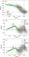 |
Fig. 8 Distribution of stars selected from GALAH DR4 in the following elemental abundance planes: (a) [Mg/Fe] − [Fe/H], (b) [Ba/Fe] − [Fe/H], (c) [Ba/Mg] − [Fe/H]. The gray dots represent the total sample, while the colored lines show running means with shaded error regions for stars from kinematic structures as labeled in the legend. Stars in Thamnos2 are shown as dots due to the low number of stars in the group. The dashed lines indicate where the x- and y-axis are equal to zero. |
List of all of the weights used for the standardized input t-SNE parameters.
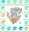 |
Fig. 9 t-SNE latent space projection of all stars in the GALAH sample, shown in gray. Halo stars from GSE and Thamnos 1 and 2 are shown in blue, green and red, respectively, while disk stars from the Splash are shown in orange. Filled points show stars identified as belonging to the halo based on the cuts applied in Figure 4, while open circles are stars selected based on their dynamics but did not pass this chemical selection. The surrounding plots show the same latent space projection, colored by various parameters. |
7 Summary
In this work, we analyzed a sample of 124 618 carefully selected red giants from the GALAH DR4 and Gaia surveys using wavelet transform and t-SNE algorithms. Our analysis revealed the following:
Using the wavelet transform technique, we were able to detect the main structures of a space defined by a square root of radial action and angular momentum; namely, the Galactic disk, Splash, GSE, Thamnos1, and Thamnos2.
The strongest detection in the wavelet maps corresponds to the Galactic disk. This is due to a large number of disk stars (112 194) in our sample. The t-SNE algorithm revealed dozens of disk structures and among them, we were able to recognize well-known moving groups in the Galactic disk.
The Splash population on the wavelet transform map plays the role of a bridge that links the metal-rich part of the Galactic disk and GSE. Because of the proximity to accreted populations in action space, these in situ stars on halo-like orbits contaminate them if selected purely based on kinematics. On the other hand, the Splash population is also contaminated by the halo stars. We observed only one peak that we link to Splash.
Our findings indicate that GSE can be divided into two substructures: the blob of accreted stars at Jr > 40 kpc km s−1 and the blob at lower values of the square root of the radial action, which is a mixture of in situ and accreted stars. We also observed that the GSE population is not purely a non-rotating component of the Galaxy. The wavelet transform showed that even when they are close to Lz ≃ 0 kpc km s−1, many stars follow slightly retrograde orbits.
In Thamnos, we discovered three peaks in the action space. Two of these peaks are combined and referred to as the Thamnos1 group. A kinematic selection of stars in the Thamnos1 group indicates that a substantial number of them belong to the high-alpha disk. However, these stars can be removed from the sample if the elemental abundances of individual stars are studied. Thamnos2, on the other hand, is mainly composed of halo stars.
An analysis of our sample with the t-SNE method using only chemical abundances as input successfully recovered the groups of stars identified with the wavelet transform. Chemical tagging could differentiate GSE, Thamnos1, and Thamnos2 from the bulk Milky Way population, but could not separate these halo structures from each other based on chemistry alone. This indicates the importance of kinematics for identifying and differentiating these structures. The t-SNE analayis also showed that the halo selection in [Mg/Cu] versus [Na/Fe] space is very effective at removing contamination when selecting stars in GSE, Thamnos1 and Thamnos2. The Splash disk is located in immediate proximity to the accreted group of stars, indicating that the Splash contaminates the selection of accreted populations.
The analysis of chemical properties of the stars in the kinematic groups was partly influenced by the way we defined the groups chemically based on Mg, Fe, Cu, and Na elemental abundances, but still allows us to conclude the following:
Although a kinematic selection only allows the choice of stars to be made among the accreted populations, an analysis of the chemical properties of these stars is needed for the ‘purest’ selection. The structures close to the Lz and with
![Mathematical equation: $\[\sqrt{J_{r}}\]$](/articles/aa/full_html/2026/05/aa51201-24/aa51201-24-eq23.png) < 25 kpc km s−1 have a higher contamination rate.
< 25 kpc km s−1 have a higher contamination rate.The peak values of metallicity distributions for each group are in agreement with the previous studies and place Splash at −0.6 dex, GSE at −1.2 dex, Thamnos1 at −1.2, and Thamnos2 at −1.3 dex. Peaks of the Galactocentric radius distributions fall into the inner Galaxy, while the GSE population covers the broadest range of Galactic radii and extends at least up to 15 kpc from the Galactic center.
Stars in the Splash exhibit chemical properties of the Galactic disk, including a high metallicity, namely, above −0.5 dex, and a relatively high abundance of iron-peak elements.
The chemical peculiarities of GSE include a low-metallicity, high [Li/Fe] abundance, and high abundance of an r-process element Sm. Surprisingly, we observed a relatively high abundance of some s-process elements, such as Ce in GSE, which does not agree with previous studies, such as Matsuno et al. (2021).
Thamnos has a slightly elevated [α/Fe] ratio than the rest of the accreted groups. Oher chemical peculiarities characterizing the Thamnos population include the abundances of Li, Ru, and Zr, which are slightly elevated than those of the rest of the groups.
In recent years, significant efforts have been made to identify and study the chemodynamical properties of the inner halo structures. The GALAH and Gaia surveys play a crucial role in searching for and analyzing kinematic parameters and elemental abundances of stars within accreted stellar populations. With these surveys, the remnants of accreted populations can be easily located in the vicinity of the Sun. A great deal of hope is vested in future spectroscopic programs to cover a broader range of Galactocentric distances, reaching as far as R > 20 kpc, to study the outer parts of the stellar halo. The high-precision spectroscopic data of future missions such as 4MOST de Jong et al. (2019) and WEAVE Dalton et al. (2018, 2020) will hopefully shed more light on the nature of these unique building blocks of our Galaxy.
Data availability
The GALAH DR4 catalog is available at https://www.galah-survey.org/dr4/overview/ and at the Strasbourg Astronomical Data Center (CDS) via https://cds.unistra.fr. We provide a supplementary table containing information for 116 047 stars with GALAH DR4 and Gaia DR3 identifiers. The column “halo” indicates whether a star belongs to the stellar halo (True) or the disk (False) based on [Mg/Cu] vs. [Na/Fe] criteria. The columns “Splash”, “GSE”, “Thamnos1”, and “Thamnos2” indicate whether a star belongs to the corresponding kinematic structure (True or False) based on the wavelet transform. The table is available at the CDS via https://cdsarc.cds.unistra.fr/viz-bin/cat/J/A+A/709/A69
Acknowledgements
We acknowledge the traditional owners of the land on which the AAT stands, the Gamilaraay people, and pay our respects to elders past and present. This work was partly supported by the Australian Research Council Centre of Excellence for All Sky Astrophysics in 3 Dimensions (ASTRO 3D) through project number CE170100013. I.K., K.Y., and K.L. acknowledge funding from the European Research Council (ERC) under the European Union’s Horizon 2020 research and innovation program (Grant Agreement No. 852977). S.B. acknowledges support from the Australian Research Council under grant number DE240100150. J.B.H. is funded by an ARC Laureate Fellowship. Z.T. acknowledges support from the Slovenian Research Agency (core funding No. P1-0188). D.Z. is funded by ARC Discovery Project DP220102254. S.L.M. acknowledges the support of the Australian Research Council through Discovery Project grant DP220102254 and the UNSW Scientia Fellowship Program.
References
- Abdurro’uf, Accetta, K., Aerts, C., et al. 2022, ApJS, 259, 35 [NASA ADS] [CrossRef] [Google Scholar]
- Antoja, T., Helmi, A., Bienayme, O., et al. 2012, MNRAS, 426, L1 [NASA ADS] [CrossRef] [Google Scholar]
- Bailer-Jones, C. A. L. 2023, AJ, 166, 269 [NASA ADS] [CrossRef] [Google Scholar]
- Bellazzini, M., Massari, D., De Angeli, F., et al. 2023, A&A, 674, A194 [NASA ADS] [CrossRef] [EDP Sciences] [Google Scholar]
- Belokurov, V., Erkal, D., Evans, N. W., Koposov, S. E., & Deason, A. J. 2018, MNRAS, 478, 611 [Google Scholar]
- Belokurov, V., Sanders, J. L., Fattahi, A., et al. 2020, MNRAS, 494, 3880 [Google Scholar]
- Bennett, M., & Bovy, J. 2019, MNRAS, 482, 1417 [NASA ADS] [CrossRef] [Google Scholar]
- Bland-Hawthorn, J., & Tepper-García, T. 2021, MNRAS, 504, 3168 [CrossRef] [Google Scholar]
- Bovy, J. 2015, ApJS, 216, 29 [NASA ADS] [CrossRef] [Google Scholar]
- Buder, S., Sharma, S., Kos, J., et al. 2021, MNRAS, 506, 150 [NASA ADS] [CrossRef] [Google Scholar]
- Buder, S., Lind, K., Ness, M. K., et al. 2022, MNRAS, 510, 2407 [NASA ADS] [CrossRef] [Google Scholar]
- Buder, S., Kos, J., Wang, X. E., et al. 2025, PASA, 42, e051 [Google Scholar]
- Conroy, C., Bonaca, A., Cargile, P., et al. 2019, ApJ, 883, 107 [NASA ADS] [CrossRef] [Google Scholar]
- Contursi, G., de Laverny, P., Recio-Blanco, A., et al. 2023, A&A, 670, A106 [NASA ADS] [CrossRef] [EDP Sciences] [Google Scholar]
- Dalton, G., Trager, S., Abrams, D. C., et al. 2018, SPIE Conf. Ser., 10702, 107021B [Google Scholar]
- Dalton, G., Trager, S., Abrams, D. C., et al. 2020, SPIE Conf. Ser., 11447, 1144714 [NASA ADS] [Google Scholar]
- de Jong, R. S., Agertz, O., Berbel, A. A., et al. 2019, The Messenger, 175, 3 [NASA ADS] [Google Scholar]
- De Silva, G. M., Freeman, K. C., Bland-Hawthorn, J., et al. 2015, MNRAS, 449, 2604 [NASA ADS] [CrossRef] [Google Scholar]
- Deason, A. J., & Belokurov, V. 2024, New A Rev., 99, 101706 [NASA ADS] [CrossRef] [Google Scholar]
- Feltzing, S., & Feuillet, D. 2023, ApJ, 953, 143 [NASA ADS] [CrossRef] [Google Scholar]
- Feuillet, D. K., Feltzing, S., Sahlholdt, C. L., & Casagrande, L. 2020, MNRAS, 497, 109 [Google Scholar]
- Feuillet, D. K., Sahlholdt, C. L., Feltzing, S., & Casagrande, L. 2021, MNRAS, 508, 1489 [NASA ADS] [CrossRef] [Google Scholar]
- Freeman, K., & Bland-Hawthorn, J. 2002, ARA&A, 40, 487 [Google Scholar]
- Gaia Collaboration (Vallenari, A., et al.) 2023, A&A, 674, A1 [NASA ADS] [CrossRef] [EDP Sciences] [Google Scholar]
- Haywood, M., Di Matteo, P., Lehnert, M. D., et al. 2018, ApJ, 863, 113 [Google Scholar]
- Helmi, A. 2020, arXiv e-prints [arXiv:2002.04340] [Google Scholar]
- Helmi, A., White, S. D. M., de Zeeuw, P. T., & Zhao, H. 1999, Nature, 402, 53 [Google Scholar]
- Helmi, A., Babusiaux, C., Koppelman, H. H., et al. 2018, Nature, 563, 85 [Google Scholar]
- Hinton, G., & Roweis, S. 2002, Adv. Neural Process. Syst., 15, 833 [Google Scholar]
- Holtzman, J. A., Hasselquist, S., Shetrone, M., et al. 2018, AJ, 156, 125 [Google Scholar]
- Horta, D., Schiavon, R. P., Mackereth, J. T., et al. 2021, MNRAS, 500, 1385 [Google Scholar]
- Horta, D., Schiavon, R. P., Mackereth, J. T., et al. 2023, MNRAS, 520, 5671 [NASA ADS] [CrossRef] [Google Scholar]
- Ji, A. P., Li, T. S., Hansen, T. T., et al. 2020, AJ, 160, 181 [NASA ADS] [CrossRef] [Google Scholar]
- Kobayashi, C., Karakas, A. I., & Lugaro, M. 2020, ApJ, 900, 179 [Google Scholar]
- Koppelman, H., Helmi, A., & Veljanoski, J. 2018, ApJ, 860, L11 [NASA ADS] [CrossRef] [Google Scholar]
- Koppelman, H. H., Helmi, A., Massari, D., Price-Whelan, A. M., & Starkenburg, T. K. 2019, A&A, 631, L9 [NASA ADS] [CrossRef] [EDP Sciences] [Google Scholar]
- Kos, J., Bland-Hawthorn, J., Freeman, K., et al. 2018, MNRAS, 473, 4612 [NASA ADS] [CrossRef] [Google Scholar]
- Kushniruk, I., & Bensby, T. 2019, A&A, 631, A47 [NASA ADS] [CrossRef] [EDP Sciences] [Google Scholar]
- Kushniruk, I., Schirmer, T., & Bensby, T. 2017, A&A, 608, A73 [NASA ADS] [CrossRef] [EDP Sciences] [Google Scholar]
- Lane, J. M. M., Bovy, J., & Mackereth, J. T. 2023, MNRAS, 526, 1209 [NASA ADS] [CrossRef] [Google Scholar]
- Lee, G., Gommers, R., Waselewski, F., Wohlfahrt, K., & O’Leary, A. 2019, J. Open Source Softw., 4, 1237 [NASA ADS] [CrossRef] [Google Scholar]
- Lindegren, L., Lammers, U., Bastian, U., et al. 2016, A&A, 595, A4 [NASA ADS] [CrossRef] [EDP Sciences] [Google Scholar]
- Matsuno, T., Hirai, Y., Tarumi, Y., et al. 2021, A&A, 650, A110 [NASA ADS] [CrossRef] [EDP Sciences] [Google Scholar]
- Molaro, P., Cescutti, G., & Fu, X. 2020, MNRAS, 496, 2902 [Google Scholar]
- Myeong, G. C., Vasiliev, E., Iorio, G., Evans, N. W., & Belokurov, V. 2019, MNRAS, 488, 1235 [Google Scholar]
- Naidu, R. P., Conroy, C., Bonaca, A., et al. 2020, ApJ, 901, 48 [Google Scholar]
- Nissen, P. E., & Schuster, W. J. 2010, A&A, 511, L10 [NASA ADS] [CrossRef] [EDP Sciences] [Google Scholar]
- Nissen, P. E., Amarsi, A. M., Skúladóttir, Á., & Schuster, W. J. 2024, A&A, 682, A116 [NASA ADS] [CrossRef] [EDP Sciences] [Google Scholar]
- Ortigoza-Urdaneta, M., Vieira, K., Fernández-Trincado, J. G., et al. 2023, A&A, 676, A140 [NASA ADS] [CrossRef] [EDP Sciences] [Google Scholar]
- Pedregosa, F., Varoquaux, G., Gramfort, A., et al. 2011, J. Mach. Learn. Res., 12, 2825 [Google Scholar]
- Ramos, P., Antoja, T., & Figueras, F. 2018, A&A, 619, A72 [NASA ADS] [CrossRef] [EDP Sciences] [Google Scholar]
- Sanders, J. L., Belokurov, V., & Man, K. T. F. 2021, MNRAS, 506, 4321 [NASA ADS] [CrossRef] [Google Scholar]
- Simpson, J. D., Martell, S. L., Buder, S., et al. 2021, MNRAS, 507, 43 [NASA ADS] [CrossRef] [Google Scholar]
- Starck, J.-L., & Murtagh, F. 2006, Astronomical Image and Data Analysis (Berlin: Springer) [Google Scholar]
- Tolstoy, E., Hill, V., & Tosi, M. 2009, ARA&A, 47, 371 [Google Scholar]
- Trick, W. H., Coronado, J., & Rix, H.-W. 2019, MNRAS, 484, 3291 [NASA ADS] [CrossRef] [Google Scholar]
- van der Maaten, L., & Hinton, G. 2008, J. Mach. Learn. Res., 1, 1 [Google Scholar]
- van der Walt, S., Schönberger, J. L., Nunez-Iglesias, J., et al. 2014, PeerJ, 2, e453 [Google Scholar]
- Youakim, K., Lind, K., & Kushniruk, I. 2023, MNRAS, 524, 2630 [Google Scholar]
- Zhao, G., Zhao, Y.-H., Chu, Y.-Q., Jing, Y.-P., & Deng, L.-C. 2012, Res. Astron. Astrophys., 12, 723 [NASA ADS] [CrossRef] [Google Scholar]
All Tables
All Figures
|
Fig. 1 Galactocentric distance, R, as a function of distance from the Galactic plane, Z, in the direction of the North Galactic Pole (NGP), Z = 90°, for 124 618 stars selected from GALAH DR4. Dashed lines show the Solar values R = 8 kpc and Z = 20.8 pc, while the yellow star shows the location of the Sun. The bin size is 0.05 × 0.05 kpc. |
| In the text | |
|
Fig. 2 Panel a: density map in Lz − |
| In the text | |
|
Fig. 3 Binned distributions of 116 047 stars selected from the GALAH DR4 in the [Mg/Cu] − [Na/Fe] plane. The bin size is 0.01 × 0.01. The dashed line shows the division of stars into the disk (below the line) and halo (above the line) stars. |
| In the text | |
|
Fig. 4 Scatter plot of all 116 047 stars selected from GALAH DR4 in the [Mg/Cu] − [Na/Fe] plane is shown in gray. The markers of different colors show stars in the following kinematic structures: Splash (Panel a, orange circles), GSE (Panel b, blue circles), Thamnos1 (Panel c, green circles), and Thamnos2 (Panel d, red circles). The dashed line is the same as on panel a and divides the stars into the disk and halo sub-samples. Percentages of the halo and disk stars in the kinematic structures are provided in each plot. |
| In the text | |
|
Fig. 5 Panel a: orbital energy plotted as a function of the angular momentum. Gray dots show a scatter plot of the total sample, while the other colors and symbols correspond to the kinematic structures detected in the legend. Chemically defined halo stars were excluded from the Splash and chemically defined disk stars were excluded from the rest of the groups. Panel b: similar to the plot in panel a, but showing the rotational velocity as a function of metallicity. |
| In the text | |
|
Fig. 6 Normalized probability density metallicity [Fe/H] with uncertainty bands for kinematic groups listed in the legend. The chemically defined halo stars were excluded from the Splash and chemicall -defined disk stars were excluded from the rest of the groups. The plot is generated using a kernel density estimation (KDE) with a bandwidth of 0.075 and a Gaussian kernel. The shaded regions around each curve represent corresponding uncertainties, which are standard deviations of 100 bootstrap samples. |
| In the text | |
|
Fig. 7 Panels a–d: individual distributions of elemental abundances for the Splash (orange box), GSE (blue box), Thamnos1 (green box), and Thamnos2 (red box), which are depicted using box plots. The analysis covers 32 chemical elements, X, related to iron, [X/Fe], and iron abundance, which is related to hydrogen, [Fe/H]. Each box plot adheres to standard conventions, with the first and third quartiles defining the box body, “whiskers” extending to minimum and maximum values, and the median shown as a black line inside each box. |
| In the text | |
|
Fig. 8 Distribution of stars selected from GALAH DR4 in the following elemental abundance planes: (a) [Mg/Fe] − [Fe/H], (b) [Ba/Fe] − [Fe/H], (c) [Ba/Mg] − [Fe/H]. The gray dots represent the total sample, while the colored lines show running means with shaded error regions for stars from kinematic structures as labeled in the legend. Stars in Thamnos2 are shown as dots due to the low number of stars in the group. The dashed lines indicate where the x- and y-axis are equal to zero. |
| In the text | |
|
Fig. 9 t-SNE latent space projection of all stars in the GALAH sample, shown in gray. Halo stars from GSE and Thamnos 1 and 2 are shown in blue, green and red, respectively, while disk stars from the Splash are shown in orange. Filled points show stars identified as belonging to the halo based on the cuts applied in Figure 4, while open circles are stars selected based on their dynamics but did not pass this chemical selection. The surrounding plots show the same latent space projection, colored by various parameters. |
| In the text | |
Current usage metrics show cumulative count of Article Views (full-text article views including HTML views, PDF and ePub downloads, according to the available data) and Abstracts Views on Vision4Press platform.
Data correspond to usage on the plateform after 2015. The current usage metrics is available 48-96 hours after online publication and is updated daily on week days.
Initial download of the metrics may take a while.