| Issue |
A&A
Volume 709, May 2026
|
|
|---|---|---|
| Article Number | A61 | |
| Number of page(s) | 18 | |
| Section | Interstellar and circumstellar matter | |
| DOI | https://doi.org/10.1051/0004-6361/202554829 | |
| Published online | 05 May 2026 | |
The coupled origin of the stellar initial mass function and multiplicity
The influence of hierarchical fragmentation on the core mass function
1
Univ. Grenoble Alpes, CNRS, IPAG,
38000
Grenoble,
France
2
Department of Astronomy, University of Florida,
PO Box 112055,
Gainesville,
FL
32611-2055,
USA
★ Corresponding author: This email address is being protected from spambots. You need JavaScript enabled to view it.
Received:
28
March
2025
Accepted:
6
March
2026
Abstract
Context. In the solar neighbourhood, the initial mass function (IMF) is canonically described by the Salpeter power-law slope for the high-mass range. As stars inherit their mass from their environment, their IMF may directly result from a core mass function (CMF) through accretion, gravitational collapse, and fragmentation. This inheritance implies that the mass of the gaseous fragments may be connected to the properties of clustered and multiple stellar systems. In these systems, mass and multiplicity are related, and this is supported by the fact that more massive primaries are observed more frequently in multiple systems.
Aims. We aim to (i) quantify the influence of the hierarchical fragmentation of cores on the resulting IMF and (ii) determine the consequences of this fragmentation on the multiplicity of the stellar systems.
Methods. To do so, we employed a scale-free hierarchical fragmentation model to investigate the stochastic fragmentation of the 2.5 kAU cores of the W43-MM2&MM3 molecular cloud, whose CMF is top-heavy. We also used this model to quantify the influence of deterministic mass-dependent fragmentation processes.
Results. The hierarchical fragmentation of gas clumps shifts the CMF towards a lower mass range and can modify its shape. The shift is quantified by both the number of fragments produced at each level of fragmentation and the mass the fragments inherit from their parental core. Starting from the top-heavy power-law CMF observed in W43-MM2&MM3, we show that at least four levels of hierarchical fragmentation are required to generate the turn-over peak of the canonical IMF. Within a radius of 0.2–2.5 kAU, massive stars (M > 10 M⊙) have on average 0.9 companions, five times fewer than low-mass stars (M < 0.1 M⊙), which are less dynamically stable and should disperse. We show that a universal IMF can emerge from mass-dependent fragmentation processes provided that more massive cores produce fewer fragments compared to lower mass cores and transfer their mass less efficiently to their fragments.
Conclusions. Hierarchical fragmentation alone, however, cannot reconcile a universal IMF with observed stellar multiplicity. We propose that fragmentation is not scale-free but operates in two distinct regimes: a mass-dependent phase establishing the Salpeter slope and a mass-independent phase setting the turn-over. Our framework provides a way to compare core sub-fragmentation in various star-forming regions and numerical simulations.
Key words: methods: analytical / methods: statistical / stars: luminosity function, mass function
© The Authors 2026
 Open Access article, published by EDP Sciences, under the terms of the Creative Commons Attribution License (https://creativecommons.org/licenses/by/4.0), which permits unrestricted use, distribution, and reproduction in any medium, provided the original work is properly cited.
This article is published in open access under the Subscribe to Open model. This email address is being protected from spambots. You need JavaScript enabled to view it. to support open access publication.
1 Introduction
The stellar initial mass function (IMF) is usually interpreted to be a probability density function (PDF) that describes the mass distribution of newly born stars, and it is widely used as a diagnostic tool by astronomers to assess star formation properties. The mathematical representation of the IMF has evolved over the years. Salpeter (1955) first parametrised the intermediate and high-mass regime (0.4 ≤ M ≤ 10 M⊙) for field stars as a power law, for which the fraction of stars ζ(M) per unit of logarithmic mass is given by ζ(M) = dN/d log M ∝ MΓ with Γ = −1.35, the so-called Salpeter slope. However, approximating the IMF with a single power law appeared to be too simple to represent the low-mass star range (M < 1 M⊙). Other functions have been proposed, such as a log-normal function (Miller & Scalo 1979; Scalo 1986), a combination of segmented broken power laws (Kroupa 2001), and even a combination of a log-normal function and a power law (Chabrier 2003). Non-segmented functions have also been introduced to describe the IMF shape (De Marchi et al. 2005; Maschberger 2013) and have the benefit of giving a smooth, continuous, and more practical description of the IMF.
Despite their mathematical differences, all of these functions share common shape properties to describe the seemingly universal distribution of stellar mass in the Milky Way (MW): (i) the Salpeter power law above one solar-mass star (M > 1 M⊙); (ii) a log-normal shape below 1 M⊙ with a turn-over mass, also called a peak, around M ≈ 0.1−0.4 M⊙ defining a characteristic mass for stars; (iii) a low-mass cut-off in the brown dwarf regime around M ≈ 0.2 M⊙ (Thies et al. 2015); and a high-mass cut-off around M ≈ 100−120 M⊙ (Weidner & Kroupa 2004; Figer 2005; Zinnecker & Yorke 2007; Kroupa et al. 2013; Tan et al. 2014). Because of the statistical consistency obtained over decades of a unique shape of the IMF within resolved stellar populations in the disc of the MW, it has been proposed that the IMF may be universal and independent of time and space (see e.g. the review of Krumholz 2014; Lee et al. 2020; Hennebelle & Grudić 2024). Hereafter, we refer such an IMF within the MW as a canonical IMF (cIMF). See Kroupa et al. 2026 and Gjergo & Kroupa 2025 for further discussions regarding the universality of the IMF.
Theoretical works have been performed to interpret the characteristics describing the shape of the cIMF. The log-normal low-mass regime can result from random multiplicative fragmentation processes (Larson 1973; Elmegreen & Mathieu 1983) but may also be inherited from the underlying gas density distribution of the parental cloud (Hennebelle & Chabrier 2008). The turnover mass depends on the physical properties of the molecular cloud that govern the structure and the dynamics of the cloud via (i) the local thermal Jeans length (Larson 1998, 2005), (ii) the supersonic turbulent pressure, (iii) the Mach number in molecular clouds (Padoan & Nordlund 2002; Padoan et al. 1997; Hopkins 2013b), and (iv) the equation of state of the gas (Lee & Hennebelle 2018). Lastly, the power-law high-mass end of the IMF may result from hierarchical density fluctuations driven by a turbulent cascade across different spatial scales (Hennebelle & Chabrier 2008; Hopkins 2013b; Guszejnov & Hopkins 2016). Other dynamical processes may also shape the high-mass end of the IMF. For example, Adams & Fatuzzo (1996) showed that the multiplicative combination of independent processes leads to a log-normal tail. However, if these processes exhibit power-law scaling, a power law can emerge. Similarly, competitive accretion models (Bonnell et al. 2001) can produce a power-law tail through mass-dependent accretion rates.
Nonetheless, possible variations in the IMF with the physical properties of the parental cloud represent a still open field of debate (e.g. Kroupa 2001; Elmegreen 2004; Weidner & Kroupa 2006; Kroupa et al. 2013; Hopkins 2018). Some studies claim to have observed IMF variations (Marks et al. 2012), specifically within starburst clusters and globular clusters (see also Scalo 1998, 2005 for a review). A number of effects, such as the limited statistical sampling, sample incompleteness, dynamical evolution, stellar evolution uncertainties, and unresolved multiple stellar systems may explain part of these variations. Such claims about IMF variations within the MW have been critically reviewed, and consequently it has been suggested that they do not appear to be statistically significant (Bastian et al. 2010). More recently, there has been more robust evidence of a ‘top-heavy’ IMF, characterised by an excess of high-mass stars (M > 1 M⊙ range) compared to the cIMF, in dwarf galaxies (Gennaro et al. 2018) and within the MW, for example, in the young nuclear cluster (Lu et al. 2013) or in the Arches cluster (Hosek et al. 2019). In addition, massive early-type galaxies appear to host a bottom-heavy IMF (Conroy et al. 2017), while their high metallicities require the IMF to be top-heavy (Yan et al. 2021). These findings raise questions about the physical conditions that allow a cloud to form stars with top-heavy or Salpeter-like IMFs. Therefore, the shape of the IMF may be the consequence of the underlying star formation processes that depend on the physical properties of the hosting cloud.
On the other hand, the mass function of pre-stellar cores, called the core mass function (CMF), observed in nearby star-forming regions resembles the cIMF, as its high-mass tail can also be described by a power law, close to the Salpeter one (Motte et al. 1998; Könyves et al. 2015; Sokol et al. 2019; Könyves et al. 2020; Suárez et al. 2021). Although recent works have pointed out the potential lack of robustness of CMF construction due to 2D spatial projection effects and spatial resolution limitation (Louvet et al. 2021; Padoan et al. 2023), a possible interpretation of the close resemblance between the CMF and the cIMF is that each core may in fact produce a single star with a constant mass conversion efficiency (Alves et al. 2007).
In massive star-forming regions imaged by the ALMA-IMF large program (among which W43-MM1 and W43-MM2&3), CMFs were recently observed with an excess of massive objects compared to the regular cIMF, resulting in shallower power-law indices at high masses (Motte et al. 2018; Pouteau et al. 2022; Nony et al. 2023; Louvet et al. 2024). Constant star formation efficiency (i.e. the fraction of core mass that collapses into a star) alone is not sufficient to recover the cIMF, as it simply induces a translation of the CMF towards lower masses. Without a star formation mechanism to recover the cIMF, the existence of such a top-heavy CMF challenges the seemingly universal IMF within our galaxy and supports its theoretical dependence on the parental gaseous environment.
To investigate the hypothesis that the stellar IMF emerges from a pre-existing CMF, two approaches can be considered. One may start from an observed IMF and reconstruct a synthetic CMF using clustering algorithms (e.g. Zhou et al. 2025) or start with a population of pre-stellar cores and map their CMF with the cIMF through collapse or fragmentation (e.g. Hopkins 2012). In this work, we adopt the latter to investigate the hypothesis that the shape of the IMF emerges from the CMF. To perform such mapping, one monitors the evolution of the mass distribution of gas structures until star formation ends, under the requirement that the cores should not sub-fragment but collapse into a single star with a given mass efficiency, without mergers. At this stage, the CMF of these non-fragmenting cores is supposed to be comparable to their stellar IMF in a one-to-one mapping. If the mass efficiency is not constant but depends on individual cores or if the cores sub-fragment, this observational correspondence is not guaranteed. On the contrary, a top-heavy CMF could yield the cIMF accounting for the suited fragmentation efficiencies, although the impact of these effects has never been quantified analytically.
Under the hypothesis that the cIMF emerges from the CMF, we expect fragmentation to determine both the spatial distribution and the multiplicity of the stellar systems formed within the cores. Multiplicity studies have shown that most stars possess a companion, as they are structured in binaries, triples, or higher-order systems (Lada & Lada 2003; Marks & Kroupa 2011; Duchêne & Kraus 2013). The proportion of multiples compared to isolated objects tends to increase with the mass of the most massive object contained in these systems. More than 80% of the most massive field stars (M > 10 M⊙) have at least one companion, while more than 80% of the low-mass stars (M < 0.1 M⊙) are single (see review of Offner et al. 2023 and Kroupa et al. 2026). These observations are supported by numerical simulations (Bate 2012; Guszejnov et al. 2017), which have established that most massive protostars form with at least one gravitationally bound companion. Other simulations, in which core fragmentation weakly depends on core mass, have succeeded in reconciling these multiplicity properties with the global shape of the cIMF (Houghton & Goodwin 2024).
In this work, we investigate whether the hierarchical fragmentation of <0.01 pc pre-stellar cores described by a CMF can shape both the cIMF and the observed stellar multiplicity. Although supersonic turbulence is inherently scale-free, Thomasson et al. (2024) showed that below 0.1 pc, turbulence becomes subsonic and that fragmentation is instead driven by thermal pressure, resulting in a scale-free process down to the formation of the first Larson core (Larson 1969). We reintroduce the mathematical framework developed by Thomasson et al. (2024) and apply it to the top-heavy CMF of Pouteau et al. (2022) composed of ≈0.01 pc cores, following a scale-free fragmentation. We assigned ad hoc numerical values to the model parameters in order to investigate the consequences of different fragmentation scenarios regardless of the underlying physical process driving fragmentation. For clarity, all acronyms and variable names used in this work are listed in Tables A.1 and A.2.
We introduce in Sect. 2 our scale-free model of fragmentation that describes the successive hierarchical sub-fragmentation at different spatial scales within a cloud and quantify the variations in a CMF under hierarchical fragmentation as a function of spatial scale. In Sect. 3, we monitor the spatial evolution of the top-heavy CMF from W43-MM2&MM3 region (Pouteau et al. 2022) described by a power-law distribution of index Γ = −0.95 in order to evaluate the influence of stochastic processes and mass repartition between fragments. We also discuss the conditions under which this top-heavy CMF fragments into the cIMF and its implications for the resulting stellar multiplicities. Next, in Sect. 4, we use this model to quantify the slope variations in any CMF considering different mass-dependent fragmentation prescriptions. Finally, in Sect. 6 we discuss the properties that hierarchical fragmentation requires to reconcile both the general shape of the cIMF and the multiplicity observed in stellar systems before concluding in Sect. 7.
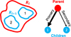 |
Fig. 1 Sketch of the hierarchical fragmentation model used. A parental object at spatial scale Rl (red) fragments into a number nl of children at scale Rl+1 (blue); here, nl = 2. The children are identified by an index i, where i = 1 represents the primary, (i.e. most massive) child. |
2 Model of hierarchical fragmentation
2.1 General framework
To investigate the influence of hierarchical fragmentation on the shape of a CMF, we aim to fragment the dense cores constituting this CMF and evaluate the resulting mass function. We use the hierarchical fragmentation model developed by Thomasson et al. (2024), which characterises the successive fragmentations of a dense gas structures across spatial scales. Fragments of size Rl+1 occupy a fragmentation level l + 1 and are embedded within larger parental structures populating the level l associated with scale Rl > Rl+1 (Fig. 1). This hierarchical process is stochastic. Stochasticity reflects the challenge of mapping a continuous gas distribution onto a discrete stellar population, which ultimately introduces an incomplete knowledge of the precise outcome of the number of fragments between two spatial scales. The number of children nl produced by one parent at the level l is random and follows a discrete probability distribution pl(nl) that assigns for each alternative nl a probability pl such that we can write its expected value  as
as
 (1)
(1)
We defined ϵl as the mass efficiency corresponding to the ratio between the total mass of the nl children and the mass of their parent (Ml):
 (2)
(2)
where Ml+1,i is the mass of the i − th child produced by one parent, with i ≤ nl (Fig. 1). Once one parent produces its nl children, the latter need to share their parental mass reservoir ϵlMl. Each child may inherit a different mass fraction from this common reservoir. The i − th child produced inherits a mass of
 (3)
(3)
where ψl,i is the fraction of mass the i − th child inherits from the parental mass reservoir. In the following, we consider a mass partition function that results in the formation of one dominant more massive fragment and other less massive (Fig. 1), or otherwise equally massive, satellite fragments:
 (4)
(4)
where q ⩾ 1 is the mass ratio between the dominant fragment and one satellite fragment. If only one child is produced, nl = 1 and the mass ratio q is by definition undefined. The Eq. (4) accounts for this case since whatever the value of q, the single child inherits all of the parental mass reservoir as ψl,i = 1. A uniform sibling mass distribution is modelled by q = 1 as all the children inherit the same fraction of the reservoir.
2.2 Scale-free fragmentation
The structure of the interstellar medium that constitutes a molecular cloud exhibits fractal properties (Elmegreen & Falgarone 1996) that reflect its self-similarity across different spatial scales. This self-similar structure in the gas is attributed to the scale-free power spectrum of turbulence that cascades through decreasing spatial scales (Hennebelle & Chabrier 2008; Guszejnov et al. 2018). However, this self-similarity does not extend over all spatial scales (Thomasson et al. 2024), as characteristic physical scales break global scale invariance (André et al. 2014). Hereafter, we describe the cloud as locally self-similar within a restricted range of spatial scales, so the degree of sub-fragmentation varies slowly with scale. This approximation can be used to identify asymptotic and general trends regarding the effect of hierarchical fragmentation.
We first introduce the fragmentation spatial rate (ϕ; Thomasson et al. 2024), which describes the rate at which the number of fragments grows between two successive spatial scales Rl+1 and Rl such that
 (5)
(5)
Next, we introduce the mass transfer spatial rate ξ (Thomasson et al. 2024) that describes the rate at which the fragment mass efficiency grows between two successive spatial scales as
 (6)
(6)
These relations ensure that for equal scale ratios r = Rl/Rl+1, the average number of fragments  produced and the mass efficiency ϵl are always the same. In a more general perspective, the choice of scale-free relations can be employed as an approximation in the case of slow variations of more complex functions ϕ(R) and ξ(R) within a sufficiently small spatial scale range such that ϕ and ξ can be considered constant.
In this framework, Thomasson et al. (2024) obtained the expression for the average mass ⟨M⟩ of individual fragments at any scale R as
 (7)
(7)
From Eq. (7), we understand that the average mass of a fragment not only depends on the mass efficiency through ξ, but also on the number of other fragments produced within the cloud through ϕ. The more the cloud fragments, the higher the number of fragments is. The flip side of this production growth is that the fragments formed are less massive as they each have access to less material. In particular, clustered fragments tend to be less massive than single fragments for the same cloud total mass.
The scale-free nature of this model dictates that sub-fragmentation continues for infinitely small scales for ϕ > 0. However, such a feature is not physical since stars have to form as a result of a gravitational collapse. Thus, it is necessary in this scale-free model to set a posteriori one stopping scale Rstop. This stopping scale sets the moment where a parental core does not sub-fragment any more and gravitationally collapses into a single star, for example, when the cores become opaque to their own radiation so non-thermal processes become dominant (Larson 1969; Lee & Hennebelle 2018) and additional fragmentation events are prevented (Thomasson et al. 2024).
2.3 Random selection of fragments
The fragmentation rate (ϕ) determines the average number of children  produced by one parent according to Eq. (5). Therefore, any choice of probability distribution pl(nl) must satisfy
 (8)
(8)
where nl can take any positive value.
For the sake of simplicity in this work, we chose to consider a binomial fragmentation process according to the following rule: A parent generates either one or two children with respective probabilities 1 − p and p. This rule is employed in Sects. 3 and 5 to investigate the detailed impact of stochastic fragmentation on the IMF and the resulting stellar systems. We exclude the case where nl = 0, as a non-existing fragment does not count in the total mass distribution of fragments. Developing Eq. (8), the probability p can be expressed as a function of the fragmentation rate (ϕ) as
 (9)
(9)
where r = Rl/Rl+1 > 1 is the scaling ratio between two successive levels. For example, to form on average  fragments, a parent has a probability 1− p = 0.7 to fragment into n = 1 child and a probability p = 0.3 to fragment into n = 2 children. Based on this binomial probability distribution the expected value
  satisfies
  for any r. According to Eq. (9), the choice of this binomial probability distribution remains valid as long as
 (10)
(10)
so that p < 1. Hereafter, we consider that as long as Eq. (10) is satisfied, fragmentation can occur, so fragments can be formed using Eq. (9).
2.4 Star formation efficiency
In our model, any spatial scale Rl may be considered as a potential scale Rstop below which fragmentation stops. In the following, we assume that each of the last fragment populating the spatial scale Rstop produces a single star. The CMF of those last fragments at Rstop would coincide with the IMF if all their mass were used to form their star. We introduce an additional average efficiency  that accounts for any star formation process below Rstop that may influence the star formation efficiency. This star formation efficiency is used to connect the mass function of the last fragmenting cores with their stellar IMF.
We defined the net star formation mass efficiency ℰ(R∗) for the cloud as the product of the cloud-to-fragments efficiency ℰ(Rstop) and the last fragments-to-star efficiency  as
as
 (11)
(11)
where ℰ(Rstop) = (Rstop/R0)−ξ from Eq. (6), provided that ξ is scale-free.
2.5 Local shape evolution
With this fragmentation framework, we evaluate the influence of hierarchical fragmentation on any mass distribution taking into account the number of objects that appear in the cloud and their formation mass efficiency. To quantify how the shape of the CMF is affected by hierarchical fragmentation, we consider an average process in which all the fragments produced constitute a macroscopic ensemble, regardless of how siblings may share their parental mass reservoir among themselves. To determine the shape evolution of the CMF with fragmentation, we defined as Γ(R, M) the local logarithmic slope of the distribution at mass
M and spatial scale R such that
 (12)
(12)
where Γ(R, M) = −1.35 corresponds to the numerical value of the Salpeter slope for M > 1 M⊙. We show in Appendix B that this local logarithmic slope Γ(R, M) is determined by
 (13)
(13)
This equation quantifies how the local logarithmic slope Γ(R, M), at a mass bin M, varies with spatial scale R during a hierarchical fragmentation process. Three terms contribute to varying this local slope.
On the left-hand side of Eq. (13), the advection term of parameter ϕ − ξ expresses the shift of the distribution along the mass domain. This advection term may reshape the distribution under some conditions described in Sect. 3.1.2. Those shape variations are investigated in more detail in Sects. 3.3 and 5 in order to derive the cIMF from a top-heavy CMF along with the resulting stellar systems.
On the right-hand side of Eq. (13), two mass derivative terms contribute to modify the local slope of the distribution. These terms account for the mass variations in both the fragmentation rate (ϕ(M)) and the mass transfer rate (ξ(M)) and are investigated analytically in Sect. 4.
3 Hierarchical fragmentation applied to a top-heavy CMF without mass dependences
In the following, we consider that both the fragmentation rate and the mass transfer rate are independent of the parental mass. Under such circumstances, only the influence of the advection term of Eq. (13) is addressed. As an experiment, the initial CMF used to derive the fragmented CMF (fCMF) is parametrised by a power law dN/d log M ∝ MΓ of index Γ = −0.95 ranging from 0.8 M⊙ to 100 M⊙. Such a top-heavy CMF has been observed by Pouteau et al. (2022) using the 1.3 and 3 mm ALMA 12 m array observation of the W43-MM2&MM3 star-forming region located at 5.5 kpc from our Sun (Zhang et al. 2014). The angular resolution of these observations is associated with a R0 = 2500 AU spatial scale resolution, below which we expect the cores to undergo scale-free fragmentation (Thomasson et al. 2024). The slope value Γ = −0.95±0.04 has been measured with robust confidence above the completeness level M ≈ 0.8 M⊙. We introduce our methodology to build the fCMF and compare it with the cIMF in Sect. 3.2. Then, in Sect. 3.3, we use this method to assess the fragmentation conditions that sufficiently reshape the initial distribution into a cIMF, and in Sect. 5 we derive the resulting stellar clustering.
3.1 Consequences of the advection term
3.1.1 Shift of the initial distribution
Considering a fragmentation process that does not depend on the parental mass, Eq. (13) simplifies into an advection equation of parameter ϕ − ξ:
 (14)
(14)
According to this advection equation, the logarithmic slope Γ(R, M) shifts along both the mass domain and the spatial scales at a rate of ϕ − ξ, which represents the mass efficiency of one individual fragment relative to its parent, considering the siblings share their parental mass reservoir (through ϕ) and that this reservoir emerges with some efficiency (through ξ), as stated in Eq. (7). Equation (14) remains valid for any subset of fragments that have been produced with the same individual mass efficiency.
3.1.2 Conditions to reshape a distribution
Each mass bin Ml+1 that constitutes the distribution on a given scale Rl+1 is built from the contributions of all the parental masses M within the scale Rl, whose possible fragmentation outcomes may generate children of mass Ml+1. Thus, the local logarithmic slope Γ(Rl+1, Ml+1) at one child bin depends on the local logarithmic slopes Γ(Rl, Ml) of every possible parental mass bin.
If the children are produced with the same individual mass efficiency, then each child mass bin is constructed from a unique parental bin. Hence, the Γ(Rl+1, Ml+1) of the different parental bins do not mix. Consequently, the distribution shifts to a different mass range, and its shape is not modified. On the contrary, if at least two parental bins yield a fragmentation outcome that produces children in the same mass bin, the global shape can change. Therefore, if parental cores produce fragments with different mass efficiencies (i.e. through q ≠ 1), or if they have multiple outcomes for their number of fragments, the shape of the distribution can be modified.
Hereafter, we consider the particular case of a power-law mass function whose logarithmic slope is constant along its mass range. Hence, ∂Γ/∂ log M = 0 in Eq. (14). Regardless of how many outcomes can contribute to a child bin, its local slope Γ(Ml+1) remains similar to the slopes of its parental bins. For the distribution to be modified, the parental distribution must be bounded in mass. In that case, some of the fragmentation outcomes that contribute to a child mass bin at the edges of the distribution may arise from unpopulated parental mass bins. On the other hand, more central child mass bins may be constructed from outcomes of populated parental bins. Then, the most extreme child bins inherit from a smaller population than their central counterparts, which effectively adds more objects to the central part of the child distribution compared to the edges, thus reshaping the distribution at its boundaries.
3.2 Method for comparing the fCMF and the cIMF
3.2.1 Generation of a fCMF
To derive the fCMF, we introduce a semi-analytic procedural method. The following method remains valid assuming (i) ϵl is not a random variable and (ii) neither the fragmentation rate (ϕ) nor mass transfer rate (ξ) depend on the mass of the parental object. The mass distribution of a population of fragments located inside any level l is described by a PDF ζl(M) normalised as
 (15)
(15)
The mass function ζl+1(M) associated with the population of the next level can be derived from ζl(M) by considering every possible fragmentation outcome of the parents constituting ζl(M). These outcomes can be categorised with respect to the number of children nl the parents may produce and the fraction of mass ϵlψl,i(nl) each individual children receive from their associated parent. For example, all i − th children originating from a nl = 2 outcome who have received the fraction ϵlψl,i(nl = 2) from their parent, constitute one sub-population of ζl+1(M). This sub-population is associated with a specific individual mass efficiency quantified by ϵlψl,i(nl = 2). At level l + 1, a sub-population is then characterised by the collection of fragments originating from the same pair (nl ; ϵlψl,i). We show in Appendix C that considering every possible pair (nl ; ϵlψl,i) the fCMF at the next level can be written as
 (16)
(16)
The construction of the mass functions of higher levels is procedural, considering each level one after the other, starting from the initial CMF at l = 0.
Statistics of the AD test and their associated significance level.
3.2.2 Statistical comparison with the cIMF
To compare our model’s fCMF with the cIMF, we used the log-logistic parametrisation by Maschberger (2013), designated as L3-cIMF. This is a non-segmented, smooth, and continuous function described by three shape parameters (γ, β, µ) and two limit parameters (ml, mu). The probability density, pL3(m), of this functional is expressed as a function of γ, β, µ:
 (17)
(17)
with G(ml, mu) a normalisation coefficient. The limits ml, mu represent respectively the lower and upper limit masses of the probability distribution pL3. The canonical parameters that describe the cIMF are given by γ = 2.3, β = 1.4 and µ = 0.2 M⊙. The parameter γ represents the logarithmic slope at large masses equivalent to the Salpeter slope. The parameter β is related to the logarithmic slope at low-masses while the parameter µ is characteristic of the peak of the cIMF. We set the range of masses starting from ml = 0.01 M⊙ onwards to mu = 150 M⊙.
This cIMF is compared with our fCMF using the Anderson-Darling (AD) test (Anderson & Darling 1954) that compares two distributions. This test is a non-parametric statistical test based on the empirical cumulative distribution that has the advantage of being equally sensitive over the whole sample range. Let H0 be the null hypothesis stating that a sample of N fragments selected from the fCMF may in fact come from the L3-cIMF distribution. The statistic A2 of this test is computed as follows:
![Mathematical equation: ${A^2} = - N - {1 \over N}\mathop \sum \limits_{i = 1}^N (2i - 1)\left[ {\ln (F({m_i})) + \ln (1 - F({m_{N - i + 1}}))} \right],$](/articles/aa/full_html/2026/05/aa54829-25/aa54829-25-eq26.png) (18)
(18)
where F(m) is the cumulative distribution function of the L3 cIMF, and mi is the i − th element of the vector m that represents the ordered masses from the smallest to the largest value within a given sample. We perform the AD test using the generic critical values with their associated significance levels (Table 1). A fCMF is considered compatible with the cIMF if we cannot reject the null hypothesis at the significance level of 0.05, that is, when the p-value is >0.05.
3.3 Retrieving the L3-cIMF from the fCMF
3.3.1 Model setup
The L3-cIMF is compared with the fCMFs derived from different sets of parameters {ϕ, ξ, q}, respectively, the fragmentation rate, the mass transfer rate and the fragment mass ratio. We monitor the evolution of the fCMF across eight levels of fragmentation from R0 = 2500 AU to R8 ≈ 98 AU. We vary ϕ between 0 and 1.5, corresponding to a fragmentation probability 0 < p < 0.84 between two successive scales ; ξ between −1 and 0.5, corresponding to efficiencies 67% < ϵl < 122%, meaning that mass accretion is possible. Each level is separated by a scaling ratio r = 1.5 in order to model a binary fragmentation between each level (see Sect. 2.3). Since we consider a scale-free process, r only regulates the number of possible fragmentation events between the initial scale R0 and the final scale Rstop. The fragments mass ratio q varies between 1 and 5. We sample the obtained fCMFs with N = 1000 objects in order to test each fCMF against the L3-cIMF from M = 10−2M⊙ up to M = 102M⊙ using the AD test. We show in Fig. 2 diagrams displaying the solutions with which H0 cannot be rejected at a 0.05 significance level.
3.3.2 Convergence to a unique shape
The AD test shows that some fCMFs are similar to the L3-cIMF (Fig. 2) when ϕ and ξ are linearly correlated, assuming a final fragments-to-star efficiency of  . This degeneracy is a consequence of Eq. (7), as the average total mass that a parent transfers to its children depends on both ξ and ϕ, such that ϕ − ξ needs to be constant to obtain the same average mass, for the same spatial scale. On the other hand, the mass ranges of the fCMF and L3-cIMF must coincide for the fCMFs to be compatible with the L3-IMF. Thus, for each spatial scale, all valid fCMF solutions are shifted by the same amount in mass. For example, panels (i) and (ii) in Fig. 2 are valid cIMF solutions, whereas panel (iii) is not.
This convergence also depends on the spatial scale Rl. As Rl decreases, solutions shift towards lower fragmentation rates and higher mass transfer rates (see e.g. panels i–iv of Fig. 2). Producing fragments of same mass at smaller scales requires keeping the fragment mass between two successive scales more efficiently, which is achieved by fragmenting less and transferring more mass to children. At a given stopping scale Rstop, this degeneracy breaks down when the average number of fragments falls below ⟨Ntot(Rstop)⟩ ≲ 2.5. Beyond that point, the resulting fCMF is indistinguishable from a scenario without fragmentation, yielding a single outcome in which one fragment is likely produced (see e.g. panel v of Fig. 2).
Although the fCMFs emerge from different sets of parameters (ϕ, ξ, q, Rstop), the resulting fCMFs exhibit similar shapes, resembling the L3-IMF. For example, panels ii and iii have different ξ and mass range but share the same shape. This implies that for any fragmentation setup, one can always find a value of  that reconciles the mass range of the fCMF with that of the cIMF. The W43-MM2&3 top-heavy CMF converges towards similar shape under mass-independent hierarchical fragmentation, suggesting that such a process yields a universal outcome, at least within the explored parameter space.
3.3.3 Limits of convergence
We recall that we assumed that ϕ and ξ are not dependent on the initial core mass. Under this assumption, a power-law CMF is reshaped if it has mass boundaries (Sect. 3.1.2), allowing variations at the distribution edges to propagate inward. In real molecular clouds, finite core samples naturally impose such boundaries, and observed CMFs rarely exhibit perfect power-law shapes due to statistical uncertainties (e.g. Enoch et al. 2007; Könyves et al. 2020; Ladjelate et al. 2020). In our case, the CMF is reshaped through the probabilistic number of fragments formed and the non-uniform mass partitioning, considering both equal-mass fragmentation (q = 1) and unbalanced cases (q > 1). A L3-IMF solution only arises for mass ratios 2 ≲ q ≲ 4 when there are fewer than seven fragmentation levels (l < 7). When q = 1, mass-independent fragmentation alone is insufficient to reshape the CMF into the L3-IMF (see panels vi and vii of Fig. 2). Thus, the mass ratio is important to efficiently modify the CMF within limited fragmentation levels.
At low masses, different fragmentation outcomes produce a log-normal cut-off, forming the IMF peak. At high masses, the distribution steepens towards the Salpeter IMF up to ≈10 M⊙, beyond which the distribution diverges from the Salpeter slope. Such a high-mass cut-off is expected from fragmentation when stochasticity is introduced (Larson 1973). In analytical theories of CMF arising from isothermal, turbulent, and/or thermally supported clouds, the location of such a cut-off at high-mass depends on the cloud Mach number (Hennebelle & Chabrier 2008). In addition, cloud sub-fragmentation appears to lower the characteristic mass of this cut-off (Hopkins 2012), as structures become comparatively less massive. However, the power-law behaviour still dominates for masses M < 100 M⊙, when the cloud Mach number is ℳ > 6.
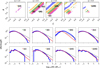 |
Fig. 2 Parameter space for which a fCMF is compatible with the Maschberger (2013) cIMF in the sense of the AD test. Top: parameter space at which a fCMF is compatible with the cIMF at a 0.05 confidence level in the fragmentation rate (ϕ) versus mass transfer rate (ξ) diagram for the mass ratio (q) of different fragments. The yellow, blue, orange, green, red, and magenta patches highlight the solutions at Rstop = 741, 494, 329, 219, 146, 98 AU after l = 3, 4, 5, 6, 7, 8 levels of fragmentation, respectively. Crosses at q = 3.0 indicate points where the average total number of fragments produced at Rstop is ≈2.5. Bottom: fragmented CMF associated with the coloured labelled points. Dashed blue, red, and black lines represent the fCMF, cIMF, and the slope of the initial top-heavy CMF, respectively. The AD test is performed from M = 0.2 M⊙ to M = 150 M⊙ to compare the fCMF with the cIMF. |
3.3.4 Beyond core fragmentation
Our study focuses on the fragmentation of compact pre-stellar cores. The framework we develop is independent of the specific fragmentation mechanism, provided that the gas multi-scale structure remains self-similar over the spatial range considered, resulting in a fragmentation rate that varies slowly within this interval. Self-similarity can be broken by a change in morphology at characteristic physical scales (e.g. filament widths, André et al. 2014) or by changes in the turbulent or thermodynamical regime (Thomasson et al. 2024). The fragmentation rate (ϕ) and mass transfer rate (ξ) are treated as free parameters, and the stochasticity reflects our limited knowledge of how mass is redistributed during fragmentation. Our framework remains applicable to various star-forming environments, including non-turbulent filaments (André et al. 2010; Hacar et al. 2017; André et al. 2019). Starting from an initial filament mass function (e.g. André et al. 2019), we can test which combinations of ϕ and ξ reproduce the observed IMF or CMF and identify the fragmentation conditions required to link the initial filamentary structure to the final stellar population. Then, these conditions can be tested against empirical measurements (Thomasson et al. 2024) or using numerical simulations in future work.
3.3.5 Brown dwarf formation
The stellar part of the IMF declines sharply around 0.2 M⊙, where the brown dwarf (BD) population emerges. Thus, the low-mass end of the cIMF likely consists of two overlapping distributions (Thies et al. 2015). In our comparison between fCMFs and the cIMF, we did not explicitly account for the contribution of BDs, which may produce a bimodal IMF (Drass et al. 2016). We assumed that all objects follow a similar formation process to the stars as supported by recent observations of proto- and pre-BD cores (Palau et al. 2024). Thus, BD cores undergo the same scale-free hierarchical fragmentation as pre-stellar cores. The discrepancy between the L3-IMF we used and the BD IMF suggests that the majority of BDs form through alternative channels (see Kroupa & Bouvier 2003; Whitworth 2018). It can also mean they go through different fragmentation regimes compared to stars, possibly involving non-scale-free behaviour, mass-dependent processes, or a stronger environmental influence.
4 Impact of mass dependences on a mass distribution
In Sect. 3 we assume the fragmentation rate and the mass transfer rate do not depend on the core mass. In fact, the chosen fragmentation prescription may depend on the local physical properties of the cloud, since all fragmentation theories involve density instabilities for a gas structure to gravitationally collapse (Jeans 1902; Hopkins 2012). In the following, we investigate the impact of mass dependences of the fragmentation rate (ϕ(M)) and mass transfer rate (ξ(M)) on the shape of the fCMF, quantified by the right-hand side of Eq. (13), so we assume  .
.
4.1 Global solution
To quantify the variation in the local slope Γ(R, M) under mass-dependent fragmentation processes only, we rewrote Eq. (13) while ignoring the advective term
 (19)
(19)
We then let  and
and  . Assuming a constant
  and
and  to assess the asymptotic trend, the solution to this differential equation is
![Mathematical equation: ${\rm{\Gamma }}(R,M) = {{\phi _M^\prime } \over {\xi _M^\prime - \phi _M^\prime }} + {\left( {{R \over {{R_0}}}} \right)^{\xi _M^\prime - \phi _M^\prime }}\left[ {{{\rm{\Gamma }}_0}(M) - {{\phi _M^\prime } \over {\xi _M^\prime - \phi _M^\prime }}} \right],$](/articles/aa/full_html/2026/05/aa54829-25/aa54829-25-eq35.png) (20)
(20)
where Γ0 is the initial logarithmic slope of the CMF at scale R0.
4.2 Effect of the mass transfer rate variations, ξ(M)
To investigate the impact of the mass transfer rate (ξ(M)) only, we set  in Eq. (20), which becomes
 (21)
(21)
If more massive objects form their fragments more efficiently in terms of mass as they are more gravitationally bound to their environment, so we can write  . The slope converges to Γ(M) = 0 as hierarchical fragmentation proceeds (as R decreases). Therefore, if
  , Γ = 0 appears as an asymptotic attractor for any initial value Γ0(M). On the contrary, if
  , the less massive cores transfer their mass more efficiently to their children. As expressed by Eq. (21), Γ diverges in this case. To complement this, we check these theoretical variation trends in Appendix D using Monte Carlo simulations, which provide good agreement with Eq. (21).
4.3 Effect of the fragmentation rate variations, ϕ(M)
To investigate the impact of the fragmentation transfer rate ϕ(M) only, we set  in Eq. (20), which becomes
![Mathematical equation: ${\rm{\Gamma }}(R,M) = [{{\rm{\Gamma }}_0}(M) + 1]{\left( {{R \over {{R_0}}}} \right)^{ - \phi _M^\prime }} - 1.$](/articles/aa/full_html/2026/05/aa54829-25/aa54829-25-eq42.png) (22)
(22)
If  , the slope converges to Γ(M) = −1 as hierarchical fragmentation continues at smaller scales. The value Γ = −1 appears as an asymptotic attractor for any initial condition Γ0(M). On the contrary, if
  , Γ diverges from the asymptotic value Γ = −1. We check these theoretical variations in Appendix D using Monte Carlo simulations, which provide good agreement with Eq. (22).
4.4 Convergence to the Salpeter IMF
In Sects. 4.2 and 4.3, we decouple the individual effects of ξ(M) and ϕ(M). We now identify more general solutions that lead a CMF to converge towards a power-law distribution. We consider the coupled influence of ξ(M) and ϕ(M). We recall that in our model, as fragmentation occurs, the spatial scale R decreases. Hereafter we focus on the asymptotic conditions R ≪ R0 under which the fragmentation processes are finished. Under these conditions, Γ(R) ≡ ΓIMF the local slope of the IMF at a given mass M. In addition, Eq. (20) converges at low scales when  . Its asymptotic limit reads as
 (23)
(23)
If we consider that the slope of the IMF corresponds to the Salpeter slope, ΓIMF = −1.35, so we obtain  . Hence, both the condition
  and Eq. (23) can be satisfied if
  , which also implies
  . Since the convergence to the Salpeter slope is independent of the initial slope Γ0, every segment of the initial CMF has the same convergence regardless of the local variations in Γ0(M) along the initial mass domain (i.e. regardless of the CMF shape).
The condition  corresponds to a fragmentation scenario in which the more massive a core is, the less it fragments. Although counter-intuitive, this perspective may be correct, as the density structure of more massive objects are more strongly determined by gravity. The density profile of these structures may tend to be statistically more radially concentrated (Shu 1977), preventing more easily the emergence of density enhancements that may grow to become unstable, for example due to turbulence (Kritsuk et al. 2011). In these conditions, more massive structures tend to sub-fragment less compared to less massive structures.
Because of gravity, we expect that more massive objects bound their surrounding material more easily. This intuitive result suggests that more massive objects fragment with a higher mass efficiency, either because of a higher infall rate (Yue et al. 2021) or because their fragments lose less material from the parental reservoir (Louvet et al. 2014). However, the condition  corresponds to a scenario in which more massive objects are less efficient in producing their fragments. This apparent opposition is a matter of definition. In our model, the mass transfer rate (ξ) is a parameter that tracks the mass efficiency (Eq. (6)). This formation efficiency is defined as the ratio between the mass of children on scale Rl+1 and the mass of their respective parents on scale Rl. In absolute value, the mass accretion rate may be higher for more massive fragments, but the proportion of accreted mass with respect to the parental mass can be lower (i.e. the mass efficiency can be lower for more massive fragments, so
  ).
).
If a universal Salpeter IMF does indeed emerge from the CMF via hierarchical fragmentation processes, both conditions  and
and  have to remain valid for the most massive objects, at least during the end of the star formation process. In this context of hierarchical fragmentation, the convergence towards the classical Salpeter IMF requires specific conditions. The processes regulating both the fragment formation efficiency and the fragmentation have to balance with
  and both
  and
and  .
.
As long as the convergence condition  is satisfied, a stable power-law distribution can naturally emerge. However, the logarithmic slope associated with this stable power law may not correspond to the Salpeter IMF if the prefactor connecting both parameters
  and
and  is different than ≈0.26. Hence, the convergence of any CMF towards a Salpeter IMF through hierarchical fragmentation remains highly circumstantial and theoretical without additional constraints on this prefactor. Outside of these convergence conditions, if
  a Salpeter IMF may still emerge from a CMF coincidentally at some stopping scale Rstop (Eq. (23) and Fig. 3).
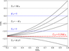 |
Fig. 3 Convergence of the local logarithmic slope Γ(R, M) under the influence of hierarchical fragmentation with the spatial scales R (solid black line) towards the Salpeter slope (dotted red line) for different initial slopes Γ0 = −2.0, −1.5, −0.5, 0, 0.5, 1.0. This convergence is only possible if |


5 Stellar systems formed through fragmentation
To build the stellar systems resulting from fragmentation and compute their properties, we perform 104 random fragmentation draws of the sample constituting the W43-MM2&MM3 CMF (Pouteau et al. 2022), with ϕ = 1.0, ξ = −0.1, q = 2 down to the scale Rstop = 219 AU, as we expect this solution to correspond to the cIMF (Sect. 3.3.2).
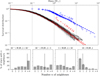 |
Fig. 4 Survival function of the fragmented CMF correlated with the multiplicity of stellar systems formed at different mass intervals. Top:104 random fragmentation draws (black lines) from the sample constituting the W43-MM2&MM3 CMF as presented in Pouteau et al. (2022, blue crosses) using the parameters ϕ = 1.0, ξ = −0.1, and q = 2. Fragmentation covers spatial scales from R0 = 2500 AU down to Rstop = 219 AU. For visibility, only the first 100 Monte Carlo draws are shown. The solid red and dashed blue line represents the cIMF and the power-law distribution fit from Pouteau et al. (2022) respectively. The dashed red line represents the average of the slopes obtained from fitting each Monte Carlo draw, using masses M > 0.8 M⊙. Bottom: distribution of the number of neighbours that a star of mass M possesses in different mass intervals (indicated above each plot). The mean value is indicated by the vertical dashed line. |
5.1 Stellar system clustering
By definition, the higher the fragmentation rate, the greater the average number of stars. At constant mass efficiency, the mass of a fragment varies inversely with its number of siblings (as 1/n; Eqs. (3) and (4)), which is a random variable. So, within a full population of fragments, the ones with the lowest masses are also those that have fragmented the most and are part of systems with the highest stellar density. In that case, stellar density refers to the number of stars located within a parental core of size R0 = 2500 AU. Hence, the most massive stars that result from non-fragmented outcomes are born in isolation. For example, stars of mass M < 0.1 M⊙ possess, on average, 4.6 neighbours in a Rcore = 2500 AU vicinity, while stars of mass M > 10 M⊙ possess 0.9 neighbours on average within the same vicinity (Fig. 4). Since the average number of fragments produced by each parent depends on the fragmentation rate, these multiplicity values also depend on the fragmentation rate. Nonetheless, the tendency to produce multiple systems of high multiplicity order with low-mass stars remains for different fragmentation rate values. Although hierarchical fragmentation inherently favours the formation of multiple systems, the more a system contains stars, the lower their mass. Yet, these multiple systems are dynamically unstable, so we expect them to quickly decay into multiple isolated stars. On the other hand, most massive objects that tend to be formed in isolation or in binaries are more stable.
5.2 Multiplicity fractions through fragmentation
The multiplicity fraction (MF) represents the fraction of stellar systems whose primary star possesses at least one companion, with a specific separation. Here, we introduce the fragmented multiplicity fraction (fMF) as the MF resulting from the sub-fragmentation of a parental core, with separations <R0. We explore the qualitative trend of the fMF, as a function of fragmentation rate mass gradient  . We can estimate a fMF as the probability that at least two stars are formed after the fragmentation process of a core. The lower the stopping scale (Rstop), the higher the fMF for each primary mass, as the parental core has more opportunities to fragment. Similarly, the higher the fragmentation rate, the higher the fMF because the probability to fragment at each level increases.
When the fragmentation rate is independent of the core mass ( ), the resulting fMF is constant with mass (see blue and black dots in Fig. 5). It reaches 100% when the fragmentation probability approaches 100%. If the gradient is positive (
 ), higher-mass cores fragment more, and the fMF increases for more massive primaries (see the green dots in Fig. 5). If the gradient is negative (
 ), higher-mass cores fragment less, and the fMF decreases for more massive primaries (see the red dots in Fig. 5).
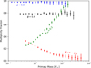 |
Fig. 5 Multiplicity fraction as a function of the primary masses grouped inside bins for different fragmentation scenarios. Each Monte Carlo simulation was carried out using 104 random cores drawn from a top-heavy CMF with Γ = −0.95 (Pouteau et al. 2022), with ξ = −0.2, q = 2, and eight levels of fragmentation. Blue and black, and green and red dots respectively represent simulations using ϕ = 0.8, ϕ = 0.4, |


6 Discussion
6.1 High-mass part of the IMF
The high-mass tail of the IMF is determined as a balance between the mass gradients of the fragmentation and the mass transfer rates (see Eq. (23)). We showed in Sect. 4.4 that a Salpeter-like IMF arises when  ,
,  , and
, and  , regardless of the shape of the initial CMF. This indicates that the fragment production efficiency increases roughly four times faster than the fragment mass efficiency for decreasing core mass. Top-heavy IMFs can be obtained by increasing the ratio
  , i.e. by increasing
  or decreasing
  . Such variations imply that top-heavy IMFs are formed through different fragmentation properties, resulting from different environmental conditions (Haslbauer et al. 2024; Zhang et al. 2018, e.g.).
More generally, we expect the high-mass slope of the IMF to vary if the ratio  fluctuates. However, if the IMF slope deviates by 10% from the Salpeter value of Γ = −1.35, we expect the ratio to vary by 29% (Eq. (23)). Consequently, the high-mass slope Γ does not appear to be highly sensitive to fluctuations in fragmentation properties. This result provides a way to test our model by comparing the fragmentation properties of regions exhibiting top-heavy, and Salpeter IMFs. Further investigation is needed to identify the physical mechanisms determining the approximative value of 0.26 for the ratio
  that is necessary to obtain a Salpeter slope in the IMF.
6.2 Multiplicity fraction
As shown in Sect. 5.2, having a negative gradient  , as requested to obtain a Salpeter-like IMF, yields to MFs that appear inconsistent with observations. In our fCMFs, the most massive mass bins are populated by fragmentation outcomes associated with a single fragment produced (nl = 1), meaning that the most massive stars are those with the lowest fMF (Fig. 4). However, the observed proportion of multiples compared to isolated stars tends to increase with the mass of the primary object contained in stellar systems (Guszejnov et al. 2017; Offner et al. 2023). This suggests that the fragmentation rate (ϕ) should be high for high-mass cores and that
  . These observational constraints have been obtained for main-sequence stars, and it has been argued that primordial MFs could be equally high for all primary masses (Kroupa et al. 2026 and references therein). In that case, we expect mass-independence of the fragmentation rate
  . Measuring the fragmentation rate for different core masses is needed to discriminate between both possibilities.
If the fragmentation rate increases significantly with the mass of the initial objects, Houghton & Goodwin (2024) found that with Γ0 > −1, the slope of the fCMF becomes too steep compared to the Salpeter slope. This steepening effect is consistent with our fragmentation model, which predicts a steepening of Γ if  . However, if ϕ(M) slowly varies with the mass (
 ), Houghton & Goodwin (2024) also showed that the slope variation is small enough to maintain the Salpeter slope while accounting for the MF of massive and low-mass primaries.
6.3 Massive star formation
If the fragmentation rate is high for high-mass cores and  as suggested above, the likelihood of cores forming massive stars decreases, thus resulting in a lower fraction of massive stars (M > 10 M⊙) in our fCMFs compared to the Salpeter IMF (see the fCMFs in Fig. 2). This depletion at high-masses can also be predicted in theoretical CMFs derived from isothermal turbulence (Hennebelle & Chabrier 2008; Hopkins 2012, 2013a), or from other probabilistic models (Elmegreen & Mathieu 1983; Zinnecker 1984). Within the framework of our model, we interpret this depletion as a consequence of the stochastic nature of our fragmentation prescription, which naturally creates a log-normal distribution (Larson 1973), influenced by the mass ratio among the fragments formed (see Sect. 3.1.2 for conditions that affect the distribution shape).
To obtain a power-law behaviour at high masses, as suggested by the CMF from both cloud observations (Nutter & Ward-Thompson 2007; Sokol et al. 2019; Cao et al. 2021; Pouteau et al. 2022) and simulations of isothermal clouds undergoing gravo-turbulent fragmentation (Schmidt et al. 2010; Guszejnov & Hopkins 2015), and to get a number of high-mass stars (M > 10 M⊙) consistent with the cIMF,  needs to be positive. This suggests that the core mass is positively correlated with the formation efficiency (Louvet et al. 2014). Such a gradient in mass effectively flattens the stellar IMF locally and increases the number of massive stars compared to lower mass stars. The fCMF then consists of a low-mass log-normal shaped population resulting from stochastic fragmentation, and a high-mass power-law-shaped population (Basu & Jones 2004), produced by a positive gradient in mass efficiency. This scenario is consistent with ≈0.1 pc CMF observed in the Cygnus-X molecular cloud (Li et al. 2021), which highlights a transition at M ≈ 10 M⊙ between a log normal and a power-law mass function composed of fragmented and accreting cores, respectively.
Moreover, having  also leads to the formation of primary objects with a higher fMF in existing stellar systems, as clustered low-mass stars may collectively accrete material from their environment while competing for it (Clark & Whitworth 2021). In this scenario, the probability of forming clustered stars with a massive primary increases, so the fMF becomes qualitatively more consistent with observations (see Sect. 6.2).
6.4 Limitation of scale-free hierarchical fragmentation
We discuss the conditions that set both the turn-over mass of the cIMF with hierarchical fragmentation and the power law at high masses. We distinguish three cases. When mass gradients remain constant and exceed stochastic contributions (Sect. 4), the resulting distribution is a power law regardless of the initial CMF. In this regime, any turn-over feature is suppressed. When mass gradients vary with mass dominate and exceed stochastic contributions, a turnover emerges at mass where  . A power-law tail at high masses is still possible, provided that the ratio
  and is constant at high mass (Fig. 3). However, in this case, our scale-free assumption no longer holds as two regimes of fragmentation are needed. When stochastic fragmentation dominates, that is, when mass the derivatives are small
  and
and  , the distribution develops log-normal features at its boundaries, with a turn-over at low masses (Sect. 3). However, without mass gradients, no power law is expected at the high-mass end.
In this scale-free framework, two modes of fragmentation are required to recover the whole shape of the IMF: the peak and the log-normal part of the IMF are determined by random, stochastic processes while the high-mass power-law part of the cIMF is determined by mass-dependent fragmentation.
We discuss here the possibility for hierarchical fragmentation to shape a Salpeter-like IMF at high masses while setting a high MF for massive primary stars. To set such an MF, we found in Sect. 6.2 that the fragmentation rate needs to be high at high masses and  . Moreover, in the context of hierarchical fragmentation, massive stars with masses M > 10 M⊙ can only form if
  (see Sect. 6.3). These two conditions are incompatible with our theoretical results from Sect. 4.4, stating that both
  and
and  are required to converge to a Salpeter IMF, unless this IMF is reached coincidentally. From this perspective, a universal IMF cannot emerge from scale-free hierarchical fragmentation alone, accounting only for deterministic mass-dependent processes.
6.5 Effect of other processes
6.5.1 Role of disc fragmentation
The shape of the IMF may be influenced by fragmentation events occurring on scales R < Rstop, below the core fragmentation stopping scales as disc fragmentation occurs. However, we do not expect disc fragmentation to significantly impact the shape of the fCMF, as a single fragmentation event marginally affects the power-law index. Since few fragmentation steps are expected, a mass dependence of the fragmentation rate ( ) should also have little influence, especially if one considers that ϕ(M) slowly varies with mass (Houghton & Goodwin 2024). At this stage, the primary factor that modifies the shape of the fCMF is through a mass-dependent mass transfer rate (
 ) for scales R < Rstop, which implies using a variable mass efficiency to map the last fragmenting cores with their stars.
Disc fragmentation also alters the multiplicities of stellar systems by producing close binaries, which could reconcile the MF of high-mass stars with observations. However, if fragmentation continues at scales smaller than Rstop < 150 AU, lower-mass cores would form and massive stars (M > 10 M⊙) would be even more difficult to form unless  is larger, as discussed above (see Sect. 6.3).
6.5.2 Impact of the local mass reservoir
In our model, we assume that the mass transfer rate (ξ(M)) does not depend on the spatial scale (R; scale-free assumption), and that it depends only on the mass (M) of the parental object. In a larger context in which cores interact dynamically with their environment, accretion processes may occur which can also depend on the gas density from which mass is accreted. From a theoretical perspective, the relationship between the spatial distribution of the fragments (of number density n ∝ r−2) and the spatial distribution of the gas reservoir (of volumetric density ρ ∝ r−2) sets the convergence of the power index of the high-mass tail of the IMF towards the value Γ = −1/2 for gas-dominated potential (Bonnell et al. 2001). As long as the mass accretion rate increases with the core mass as Ṁ ∝ Mx with x > 1, we expect that  since the initial core mass grows faster the more massive it is (otherwise we expect
  ). However, because of the fluctuating availability of the local accretion reservoir of the cores that depends on their position in the cloud (Ballesteros-Paredes et al. 2015), it is possible that
  . In addition, when considering temporal aspects, the condition
  is not necessarily verified if some objects deplete their accretion reservoir before the others. For example, if more massive objects stop accreting at time t while the less massive ones continue to grow (Maschberger et al. 2014), we have
  . These couplings between the core mass, the available accretion reservoir, and the duration for which this reservoir remains available could re-balance the high-mass tail of the IMF to −1 (Ballesteros-Paredes et al. 2015).
6.5.3 Dynamical interactions
In addition, core-to-core mutual interactions may also modify the fragmentation properties and induce evolutionary effects. For example, if more massive structures fragment more at time t0 (i.e.  ), the resulting gas fragments become more clustered, which may enhance the probability of core coalescence (Inutsuka & Miyama 1997). According to recent numerical simulations, one third of the cores are suspected to experience coalescence, indicating that it is a frequent and important phenomenon (Offner et al. 2022). In that case, more massive parents possess more clustered cores that subsequently merge more frequently, resulting in comparatively fewer fragments at a later time. Thus, the fragmentation rate effectively satisfies
  . The complex dynamic associated with coalescence gas processing may also induce more gas to be removed from the initial parent, so the mass transfer rate may also effectively satisfy
  . These considerations need to be more deeply quantified to describe the full scenario of fragments formation.
6.5.4 Stellar feedback
Alternatively, stellar feedback from the first-born massive stars can locally prevent further fragmentation (Myers et al. 2013) and expel gas material from the cores. In addition, Zhou et al. (2025) showed that lower-mass cores in the W43-MM2&MM3 regions need to have higher mass efficiency in order to match the stellar IMF. This result is compatible with a  scenario. This would imply a dependence of the fragmentation properties on the evolutionary stage of the cloud. In order to have a universal high mass slope, both conditions
  and
and  may arise during the latest stages of core evolution and/or star formation, specifically for the cores hosting the stars of the Salpeter part of the IMF. In that case, if we only account for core hierarchical fragmentation, the Salpeter slope would be intrinsically connected to the physics of massive stars at the latest stages of star formation, while MFs would be a remnant of earlier phases of star formation when no radiative feedback takes place, with
  .
.
6.5.5 Two phases of fragmentation?
Following the above discussion, we propose that star formation occurs in two phases. During the early phases of core evolution, fragmentation occurs with  and
and  and sets the multiplicity properties of future stellar systems. Those conditions result in top-heavy CMF with slopes Γ > −1. Then, as these conditions revert in later stages due to dynamical interactions and stellar feedback, we expect the slope Γ to decrease with Γ < −1.
7 Conclusion
We have applied the fragmentation model framework from Thomasson et al. (2024) to investigate the scale-free fragmentation of pre-stellar cores. In particular, we discussed the means to recover both the cIMF and the observed multiplicity of stellar systems in scenarios in which only hierarchical fragmentation occurs. To quantify the resulting mass distribution of a stellar population and their clustering as stellar groups, the gas cloud was structured on several spatial scales equivalent to fragmentation levels. We defined (i) the fragmentation spatial rate ϕ, which determines the number of fragments produced at each scale; (ii) the mass transfer spatial rate ξ, which describes the efficiency with which the parental structure sub-fragments at each scale; (iii) the mass partition of the fragments q > 1, which regulates the mass distribution between fragments at one level; and (iv) the scale Rstop, below which fragmentation ends. We restate that all acronyms and variable names used throughout this work are listed in Tables A.1 and A.2, respectively.
We distinguished two contributions that influence the shape of the CMF during hierarchical fragmentation. First, we investigated the impact of stochastic hierarchical fragmentation with ξ and ϕ independent of the mass. We mapped the spatial evolution of a top-heavy CMF extracted from the W43-MM2&MM3 ridge (Pouteau et al. 2022) across the scales, starting from R0 = 2500 AU down to a varying Rstop. Second, we quantified the slope variations in a CMF when the fragmentation rate (ϕ(M)) and the mass transfer rate (ξ(M)) are dependent on the core mass (M). Using this fragmentation model, we showed the following:
The shift of the CMF towards lower masses is quantified by the fragmentation rate and the mass transfer rate.
Fragmentation processes that are independent of mass produce IMFs with the same shape, with mass partitions 2 < q < 4 and average number of fragments greater than 2.5.
The resulting IMFs are inconsistent with the formation of high-mass stars, because of the log-normal cut-off at masses M > 10 M⊙, and the MFs of stellar systems, as most massive fragments possess five times fewer companions than the least massive ones.
A universal Salpeter IMF emerges from hierarchical fragmentation if the fragmentation rate and the mass transfer rate depend on the mass of the initial core, such as
 , with
  and
and  .
.Multiplicity fractions increase with primary mass if
 . Massive stars are likely formed if
  .
.
The last two points in the list contradict each other. Therefore, scale-free hierarchical fragmentation alone cannot simultaneously reproduce both the full shape of the cIMF (at low and high mass) and the observed stellar multiplicity.
One possibility is that fragmentation is in fact not scale-free. With that perspective, we suggest that star formation occurs in two phases. During the initial phase, more massive cores fragment more ( ), with higher mass efficiencies (
 ). This phase seeds the multiplicity of the upcoming stellar systems. During the second phase, core dynamics and radiative feedback from the first-born massive stars may prevent further fragmentation (i.e.
  ), which may also result in lower mass efficiency (i.e.
  ) for more massive cores. In such a scenario, the Salpeter slope is determined by mass-dependent processes, while the low-mass part of the IMF is shaped by mass-independent fragmentation, for which
  and
and  , down to 10−2 M⊙.
Alternatively, scale-free fragmentation may reproduce only the cIMF, while clustering of massive stars would be determined by stellar dynamics after star formation has taken place. In that case, more massive, less clustered stars constitute more stable systems than more clustered, less massive ones. This hypothesis needs to be investigated using stellar systems formed through scale-free fragmentation as initial conditions for simulations of cluster dynamical evolution.
To investigate the origin of the stellar IMF from any CMF, detailed information about individual core properties is necessary to accurately map both mass functions, whether these cores sub-fragment or constitute the last fragmenting structures before the formation of individual stars. We have addressed the theoretical aspect of hierarchical fragmentation, although we lack quantitative multi-scale measurements to assess the mass dependence of the fragmentation rate and the mass transfer rate. Nonetheless, we provide a general framework as a basis for such measurements, and we have investigated the influence of fragmentation on the relationship between the shape of the IMF and the underlying stellar clusters. The fragmentation rate and the mass transfer rate can also be used as observable metrics to test our model prediction and to quantitatively compare core sub-fragmentation in star-forming regions and numerical simulations.
Acknowledgements
B.T. carried out this project under equal supervision of I.J. and E.M. who both provided comments and suggestions on this manuscript. F.M., T.Y. and A.G. provided helpful discussion and comments on the paper. B.T., I.J. and F.M. have received financial support from the French Agence Nationale de la Recherche (ANR) through the project “COSMHIC” (ANR-20-CE31-0009) and the “StarFormMapper” project funded by the European Union’s Horizon 2020 Research and Innovation Action programme (Grant 687528). B.T. acknowledges the ALMA-IMF consortium (ALMA project #2017.1.01355.L) for providing data and useful discussion on this work. We thank the anonymous referee for their helpful comments and careful review, which helped us improve the manuscript.
References
- Adams, F. C., & Fatuzzo, M. 1996, ApJ, 464, 256 [NASA ADS] [CrossRef] [Google Scholar]
- Alves, J., Lombardi, M., & Lada, C. J. 2007, A&A, 462, L17 [NASA ADS] [CrossRef] [EDP Sciences] [Google Scholar]
- Anderson, T. W., & Darling, D. A. 1954, J. Am. Stat. Assoc., 49, 765 [Google Scholar]
- André, P., Men’shchikov, A., Bontemps, S., et al. 2010, A&A, 518, L102 [NASA ADS] [CrossRef] [EDP Sciences] [Google Scholar]
- André, P., Di Francesco, J., Ward-Thompson, D., et al. 2014, in Protostars and Planets VI, eds. H. Beuther, R. S. Klessen, C. P. Dullemond, & T. Henning (Tucson: University of Arizona Press), 27 [Google Scholar]
- André, P., Arzoumanian, D., Könyves, V., Shimajiri, Y., & Palmeirim, P. 2019, A&A, 629, L4 [Google Scholar]
- Ballesteros-Paredes, J., Hartmann, L. W., Pérez-Goytia, N., & Kuznetsova, A. 2015, MNRAS, 452, 566 [NASA ADS] [CrossRef] [Google Scholar]
- Bastian, N., Covey, K. R., & Meyer, M. R. 2010, Ann. Rev. Astron. Astrophys., 48, 339 [Google Scholar]
- Basu, S., & Jones, C. E. 2004, MNRAS, 347, L47 [NASA ADS] [CrossRef] [Google Scholar]
- Bate, M. R. 2012, MNRAS, 419, 3115 [NASA ADS] [CrossRef] [Google Scholar]
- Bonnell, I. A., Clarke, C. J., Bate, M. R., & Pringle, J. E. 2001, MNRAS, 324, 573 [NASA ADS] [CrossRef] [Google Scholar]
- Cao, Y., Qiu, K., Zhang, Q., Wang, Y., & Xiao, Y. 2021, ApJ, 918, L4 [NASA ADS] [CrossRef] [Google Scholar]
- Chabrier, G. 2003, PASP, 115, 763 [Google Scholar]
- Clark, P. C., & Whitworth, A. P. 2021, MNRAS, 500, 1697 [Google Scholar]
- Conroy, C., van Dokkum, P. G., & Villaume, A. 2017, ApJ, 837, 166 [NASA ADS] [CrossRef] [Google Scholar]
- De Marchi, G., Paresce, F., & Portegies Zwart, S. 2005, Astrophys. Space Sci. Lib., 327, 77 [NASA ADS] [CrossRef] [Google Scholar]
- Drass, H., Haas, M., Chini, R., et al. 2016, MNRAS, 461, 1734 [NASA ADS] [CrossRef] [Google Scholar]
- Duchêne, G., & Kraus, A. 2013, Ann. Rev. Astron. Astrophys., 51, 269 [CrossRef] [Google Scholar]
- Elmegreen, B. G. 2004, MNRAS, 354, 367 [NASA ADS] [CrossRef] [Google Scholar]
- Elmegreen, B. G., & Falgarone, E. 1996, ApJ, 471, 816 [NASA ADS] [CrossRef] [Google Scholar]
- Elmegreen, B. G., & Mathieu, R. D. 1983, MNRAS, 203, 305 [NASA ADS] [CrossRef] [Google Scholar]
- Enoch, M. L., Glenn, J., I. Evans, Neal J., et al. 2007, ApJ, 666, 982 [NASA ADS] [CrossRef] [Google Scholar]
- Figer, D. F. 2005, Nature, 434, 192 [Google Scholar]
- Gennaro, M., Tchernyshyov, K., Brown, T. M., et al. 2018, ApJ, 855, 20 [NASA ADS] [CrossRef] [Google Scholar]
- Gjergo, E., & Kroupa, P. 2025, Nucl. Phys. B, 1017, 116931 [Google Scholar]
- Guszejnov, D., & Hopkins, P. F. 2015, MNRAS, 450, 4137 [NASA ADS] [CrossRef] [Google Scholar]
- Guszejnov, D., & Hopkins, P. F. 2016, MNRAS, 459, 9 [Google Scholar]
- Guszejnov, D., Hopkins, P. F., & Krumholz, M. R. 2017, MNRAS, 468, 4093 [CrossRef] [Google Scholar]
- Guszejnov, D., Hopkins, P. F., & Grudić, M. Y. 2018, MNRAS, 477, 5139 [NASA ADS] [CrossRef] [Google Scholar]
- Hacar, A., Tafalla, M., & Alves, J. 2017, A&A, 606, A123 [NASA ADS] [CrossRef] [EDP Sciences] [Google Scholar]
- Haslbauer, M., Yan, Z., Jerabkova, T., et al. 2024, A&A, 689, A221 [NASA ADS] [CrossRef] [EDP Sciences] [Google Scholar]
- Hennebelle, P., & Chabrier, G. 2008, ApJ, 684, 395 [Google Scholar]
- Hennebelle, P., & Grudić, M. Y. 2024, ARA&A, 62, 63 [Google Scholar]
- Hopkins, P. F. 2013a, MNRAS, 430, 1653 [NASA ADS] [CrossRef] [Google Scholar]
- Hopkins, P. F. 2013b, MNRAS, 433, 170 [Google Scholar]
- Hopkins, A. M. 2018, PASA, 35, e039 [NASA ADS] [CrossRef] [Google Scholar]
- Hopkins, P. F. 2012, MNRAS, 423, 2037 [NASA ADS] [CrossRef] [Google Scholar]
- Hosek, Matthew W., J., Lu, J. R., Anderson, J., et al. 2019, ApJ, 870, 44 [NASA ADS] [CrossRef] [Google Scholar]
- Houghton, R. J., & Goodwin, S. P. 2024, MNRAS, 531, 3373 [Google Scholar]
- Inutsuka, S.-i., & Miyama, S. M. 1997, ApJ, 480, 681 [NASA ADS] [CrossRef] [Google Scholar]
- Jeans, J. H. 1902, Phil. Trans. R. Soc. London Ser. A, 199, 1 [Google Scholar]
- Könyves, V., André, P., Men’shchikov, A., et al. 2015, A&A, 584, A91 [Google Scholar]
- Könyves, V., André, P., Arzoumanian, D., et al. 2020, A&A, 635, A34 [Google Scholar]
- Koziol, J. A. 1987, J. Educational Stat., 12, 412 [Google Scholar]
- Kritsuk, A. G., Norman, M. L., & Wagner, R. 2011, ApJ, 727, L20 [NASA ADS] [CrossRef] [Google Scholar]
- Kroupa, P. 2001, MNRAS, 322, 231 [NASA ADS] [CrossRef] [Google Scholar]
- Kroupa, P., & Bouvier, J. 2003, MNRAS, 346, 369 [NASA ADS] [CrossRef] [Google Scholar]
- Kroupa, P., Weidner, C., Pflamm-Altenburg, J., et al. 2013, Planets, Stars and Stellar Systems (Berlin: Springer), Galactic Structure and Stellar Populations, eds. T. D. Oswalt, & G. Gilmore, 5, 115 [Google Scholar]
- Kroupa, P., Gjergo, E., Jerabkova, T., & Yan, Z. 2026, Encyclopedia of Astrophysics (Berlin: Springer), 2, 173 [Google Scholar]
- Krumholz, M. R. 2014, Phys. Rep., 539, 49 [Google Scholar]
- Lada, C. J., & Lada, E. A. 2003, ARA&A, 41, 57 [Google Scholar]
- Ladjelate, B., André, P., Könyves, V., et al. 2020, A&A, 638, A74 [NASA ADS] [CrossRef] [EDP Sciences] [Google Scholar]
- Larson, R. B. 1969, MNRAS, 145, 271 Larson, R. B. 1973, MNRAS, 161, 133 [Google Scholar]
- Larson, R. B. 1998, MNRAS, 301, 569 [NASA ADS] [CrossRef] [Google Scholar]
- Larson, R. B. 2005, MNRAS, 359, 211 [CrossRef] [Google Scholar]
- Lee, Y.-N., & Hennebelle, P. 2018, A&A, 611, A89 [NASA ADS] [CrossRef] [EDP Sciences] [Google Scholar]
- Lee, Y.-N., Offner, S. S. R., Hennebelle, P., et al. 2020, Space Sci. Rev., 216, 70 [NASA ADS] [CrossRef] [Google Scholar]
- Li, G.-X., Cao, Y., & Qiu, K. 2021, ApJ, 916, 13 [NASA ADS] [CrossRef] [Google Scholar]
- Louvet, F., Motte, F., Hennebelle, P., et al. 2014, A&A, 570, A15 [NASA ADS] [CrossRef] [EDP Sciences] [Google Scholar]
- Louvet, F., Hennebelle, P., Men’shchikov, A., et al. 2021, A&A, 653, A157 [NASA ADS] [CrossRef] [EDP Sciences] [Google Scholar]
- Louvet, F., Sanhueza, P., Stutz, A., et al. 2024, A&A, 690, A33 [NASA ADS] [CrossRef] [EDP Sciences] [Google Scholar]
- Lu, J. R., Do, T., Ghez, A. M., et al. 2013, ApJ, 764, 155 [NASA ADS] [CrossRef] [Google Scholar]
- Marks, M., & Kroupa, P. 2011, MNRAS, 417, 1702 [NASA ADS] [CrossRef] [Google Scholar]
- Marks, M., Kroupa, P., Dabringhausen, J., & Pawlowski, M. S. 2012, MNRAS, 422, 2246 [NASA ADS] [CrossRef] [Google Scholar]
- Maschberger, T. 2013, MNRAS, 429, 1725 [NASA ADS] [CrossRef] [Google Scholar]
- Maschberger, T., Bonnell, I. A., Clarke, C. J., & Moraux, E. 2014, MNRAS, 439, 234 [Google Scholar]
- Miller, G. E., & Scalo, J. M. 1979, ApJS, 41, 513 [Google Scholar]
- Motte, F., Andre, P., & Neri, R. 1998, A&A, 336, 150 [NASA ADS] [Google Scholar]
- Motte, F., Nony, T., Louvet, F., et al. 2018, Nat. Astron., 2, 478 [Google Scholar]
- Myers, A. T., McKee, C. F., Cunningham, A. J., Klein, R. I., & Krumholz, M. R. 2013, ApJ, 766, 97 [Google Scholar]
- Nony, T., Galván-Madrid, R., Motte, F., et al. 2023, A&A, 674, A75 [NASA ADS] [CrossRef] [EDP Sciences] [Google Scholar]
- Nutter, D., & Ward-Thompson, D. 2007, MNRAS, 374, 1413 [Google Scholar]
- Offner, S. S. R., Taylor, J., Markey, C., et al. 2022, MNRAS, 517, 885 [NASA ADS] [CrossRef] [Google Scholar]
- Offner, S. S. R., Moe, M., Kratter, K. M., et al. 2023, ASP Conf. Ser., 534, 275 [NASA ADS] [Google Scholar]
- Padoan, P., & Nordlund, Å. 2002, ApJ, 576, 870 [NASA ADS] [CrossRef] [Google Scholar]
- Padoan, P., Nordlund, A., & Jones, B. J. T. 1997, MNRAS, 288, 145 [NASA ADS] [CrossRef] [Google Scholar]
- Padoan, P., Pelkonen, V. M., Juvela, M., Haugbølle, T., & Nordlund, Å. 2023, MNRAS [arXiv:2301.07398] [Google Scholar]
- Palau, A., Huélamo, N., Barrado, D., Dunham, M. M., & Lee, C. W. 2024, New A Rev., 99, 101711 [Google Scholar]
- Pouteau, Y., Motte, F., Nony, T., et al. 2022, A&A, 664, A26 [NASA ADS] [CrossRef] [EDP Sciences] [Google Scholar]
- Salpeter, E. E. 1955, ApJ, 121, 161 [Google Scholar]
- Scalo, J. 1998, ASP Conf. Ser., 142, 201 [Google Scholar]
- Scalo, J. 2005, Astrophys. Space Sci. Lib., 327, 23 [Google Scholar]
- Scalo, J. M. 1986, Fund. Cosmic Phys., 11, 1 [NASA ADS] [EDP Sciences] [Google Scholar]
- Schmidt, W., Kern, S. A. W., Federrath, C., & Klessen, R. S. 2010, A&A, 516, A25 [NASA ADS] [CrossRef] [EDP Sciences] [Google Scholar]
- Shu, F. H. 1977, ApJ, 214, 488 [Google Scholar]
- Sokol, A. D., Gutermuth, R. A., Pokhrel, R., et al. 2019, MNRAS, 483, 407 [NASA ADS] [CrossRef] [Google Scholar]
- Suárez, G., Galván-Madrid, R., Aguilar, L., et al. 2021, ApJ, 921, 48 [Google Scholar]
- Tan, J. C., Beltrán, M. T., Caselli, P., et al. 2014, in Protostars and Planets VI, eds. H. Beuther, R. S. Klessen, C. P. Dullemond, & T. Henning (Tucson: University of Arizona Press), 149 [Google Scholar]
- Thies, I., Pflamm-Altenburg, J., Kroupa, P., & Marks, M. 2015, ApJ, 800, 72 [NASA ADS] [CrossRef] [Google Scholar]
- Thomasson, B., Joncour, I., Moraux, E., et al. 2024, A&A, 689, A133 [NASA ADS] [CrossRef] [EDP Sciences] [Google Scholar]
- Weidner, C., & Kroupa, P. 2004, MNRAS, 348, 187 [NASA ADS] [CrossRef] [Google Scholar]
- Weidner, C., & Kroupa, P. 2006, MNRAS, 365, 1333 [Google Scholar]
- Whitworth, A. 2018, arXiv e-prints [arXiv:1811.06833] [Google Scholar]
- Yan, Z., Jeřábková, T., & Kroupa, P. 2021, A&A, 655, A19 [NASA ADS] [CrossRef] [EDP Sciences] [Google Scholar]
- Yue, Y.-H., Qin, S.-L., Liu, T., et al. 2021, Res. Astron. Astrophys., 21, 014 [CrossRef] [Google Scholar]
- Zhang, B., Moscadelli, L., Sato, M., et al. 2014, ApJ, 781, 89 [Google Scholar]
- Zhang, Z.-Y., Romano, D., Ivison, R. J., Papadopoulos, P. P., & Matteucci, F. 2018, Nature, 558, 260 [Google Scholar]
- Zhou, J. W., Kroupa, P., & Dib, S. 2025, A&A, 695, L17 [NASA ADS] [CrossRef] [EDP Sciences] [Google Scholar]
- Zinnecker, H. 1984, MNRAS, 210, 43 [Google Scholar]
- Zinnecker, H., & Yorke, H. W. 2007, ARA&A, 45, 481 [Google Scholar]
Appendix A Definitions
In this appendix we show useful tables in which all acronyms (Table A.1) and the relevant model parameters (Table A.2) we use in text are listed and defined.
Acronyms used throughout the article.
Appendix B Variation in the number of fragments
The purpose of this appendix is to derive Eq. 13 we introduce in Sect. 4 that characterises the variation in the local power index Γ(R, M) after a series of fragmentation events throughout the spatial scales R, at mass M. Consider the number of fragments N(R, M) of mass M and size R. In the logarithmic space, it is always possible to locally characterise such a function from the slope Γ(R, M) which represents the tangent line of the function log N(R, M) with respect to its logarithmic in of mass log M by
 (B.1)
(B.1)
Assuming the mass variations in Γ(R, M) are small in an interval d log M, we can locally approximate the function N(R, M) by N(R, M) ∝ MΓ. On the other hand, the mass distribution at one spatial scale R is defined as the number of fragments counted within a finite mass interval and we can show that
 (B.2)
(B.2)
Therefore, the power index Γ(R, M) describes the number of fragments within a small mass interval of d log M. As long as we consider local variations in mass, this description remains valid. For example, the Salpeter power-law index Γ = 1.35 quantifies the local variations in the IMF within the M > 1 M⊙ mass range.
To assess the variations in the local index Γ(R, M) at mass M along fragmentation events that cascade through spatial scales R, we take the following derivative with Eq. B.1:
 (B.3)
(B.3)
where we use the symmetry of second derivatives. We then need to compute the variation in the number of fragments of mass M between two successive scales.
We assume that only the parental objects of mass Mp can form children of mass M. Hence, the number of children produced at scale Rl+1 corresponds to the number of parents at scale Rl (with mass Mp) multiplied by their average number of children  created (see Fig. B.1):
 (B.4)
(B.4)
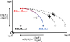 |
Fig. B.1 Schematic view of the number of children of mass Ml+1 created at the scale Rl+1 (red dot) from one parental object of mass Ml at scale Rl (blue dot). In this work we assume that children result from the outcome of a single parental mass (solid coloured line) and neglect other possible contributions (crossed dotted lines). Since only the blue dot injects children in the red dot, the number of fragments inside the red dot corresponds to the number of parents inside the blue dot multiplied by the average number of fragments |

We also recall Eq. 5 that quantifies the average number of fragments produced  between two scales by one parent with the fragmentation rate (ϕ):
 (B.5)
(B.5)
This equation can be extended by considering the individual fragmentation rate (ϕ(M)) that depends on the mass of the parental object.
Next, we approximate the derivative of ∂ log N/∂ log R as
 (B.6)
(B.6)
Using Eq. B.4 we obtain
 (B.7)
(B.7)
which can be written as
 (B.8)
(B.8)
We recognise the first term as being the local slope Γ(R, M) and the third term can be simplified using Eq. B.5 as
 (B.9)
(B.9)
Definitions of the relevant variables.
Since the parental mass Mp lies at the spatial scale Rl+1 while the children mass M lies at the scale Rl, we can write
 (B.10)
where  is the mass variation between a parent its child of mass M between two successive levels of fragmentation. The component ϕ reflects the fact that multiple fragments of mass M come from the same parental mass. Then, we can substitute Eq. B.10 into Eq. B.3:
 (B.11)
Within the framework of our model, the mass variation δM between a parent and a child is given using Eq. 3 by
 (B.12)
so the pace δM quantifies by how much mass one fragment is shifted from its original parental mass bin through the spatial scales.
Assuming that all the children are formed with the same mass efficiency, we can consider an average slope variation and δM ≈ ϕ − ξ (see Eq. 7) which reads
 (B.13)
This equation is analogous to an advection equation in which the local slope Γ(R, M) is transported throughout the mass domain M with successive fragmentation events across the spatial scales R at a pace ϕ − ξ. Two additional terms describe the influence of mass dependences on the evolution of the local slope Γ(R, M).
Appendix C Procedural generation of a fCMF
We derive the Eq. 16 used to procedurally compute the fCMF at a specific spatial scale in Appendix C.1, and we compare the resulting fCMF with the log-normal CMF of Larson (1973) and a Monte Carlo sampling in Appendix C.2 to check the validity of our method.
Appendix C.1 Derivation of Eq. 16
To hierarchically fragment a mass distribution and derive the resulting fCMF, we introduce a semi-analytic procedural method. The following method remains valid assuming (i) ϵl is not a random variable and (ii) both the fragmentation rate (ϕ) and mass transfer rate (ξ) do not depend on the mass of the parental object. The mass distribution of a population of fragments located inside any level l is described by a PDF ζl(M) normalised as
 (C.1)
(C.1)
The mass function ζl+1(M) associated with the population of the next level can be derived from ζl(M) by considering every possible fragmentation outcome of the parents constituting ζl(M). These parents can be grouped into different sub-populations, depending on the number of children (nl) they produce and the fraction of mass (ϵlψl,i(nl)) each individual child receives from their associated parent. For example, all the i − th children originating from a nl = 2 outcome who have received the fraction ϵlψl,i(nl = 2) from their parent, constitute one sub-population of ζl+1(M). At level l + 1, a sub-population is then characterised by the collection of fragments originating from the same pair (nl ; ϵlψl,i).
On one hand, the number of children within a sibling-hood of nl fragments is Ntot(Rl) × nl × pl, where Ntot is the total number of parents at scale Rl. Since there is exactly nl children in the sibling-hood, the number of children that are produced with the efficiency ϵlψl,i in such sibling-hood is Ntot(Rl) × nl × pl/nl. This is the number of children constituting the sub-population associated with the pair (nl; ϵlψl,i). On the other hand, the total number of children produced considering every possible outcome is  , where
  is given in Eq. 1 as the expected value of the probability distribution pl. The probability νl of randomly drawing a fragment from the sub-population characterised by the pair (nl; ϵlψl,i) is the ratio between the number of children constituting this sub-population with the total number of children produced considering every outcome, which is
 (C.2)
(C.2)
We checked the probability νl(nl) is normalised by summing over all of the possible sub-populations, associated with the possible outcome pairs (nl ; ϵlψl,i):
 (C.3)
(C.3)
The mass of the children constituting any sub-population is related to the mass of their parent by Ml+1,i(nl) = ϵlψl,i(nl)Ml. Therefore, to generate the corresponding sub-population at scale l + 1 the mass of the parents at scale l is reduced by a factor ϵlψl,i(nl). We can write the expression of the PDF ζl+1(M) by summing the mass contributions of each of the sub-populations weighted by their probability of occurrence:
 (C.4)
(C.4)
where we can show that  is the normalisation coefficient and we finally obtain
 (C.5)
(C.5)
Appendix C.2 Reliability of our procedure
The scale-free model we introduce is a generalisation of the stochastic model developed by Larson (1973), later L73. Both of these models formalise the fragmentation process along several discrete fragmentation levels in which each parent randomly fragments at the next level. In L73’s model, an object of mass M0 at the initial level l = 0 has a probability p of fragmenting into two children of equal mass M0/2 towards the level l = 1, and a probability 1 − p of collapsing into a single child of mass M0. After l levels of fragmentation, the children can only acquire discrete mass values Mn = 2−nM0, where n ≤ l is the number of fragmentation events that have occurred after l levels. With their model, L73 shows that the fraction f (n, l) of the cloud mass falling into fragments of mass Mn = 2−nM0 after l fragmentation levels is given by the binomial distribution
 (C.6)
(C.6)
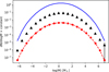 |
Fig. C.1 Mass functions derived from our scale-free fragmentation model (blue), the Larson (1973) model (L73; red), and a Monte Carlo procedure (black). The mass functions are computed under the same condition as L73 with a pseudo-Dirac as a starting mass distribution centred at 103M⊙, 19 levels of fragmentation, mass transfer rate ξ = 0 and fragments mass ratio q = 1. At each level of fragmentation the objects subdivide into one or two fragments with respective probabilities 0.5 and 0.5. The different mass functions are multiplied by different constants to separate them for better visibility. |
If N(Mn) is the number of fragments inheriting a mass Mn, the fraction f (n, l) can be written by definition as
 (C.7)
(C.7)
Hence, the number of fragments of mass Mn after l levels of fragmentation is
 (C.8)
(C.8)
With the previous equation, we can obtain the discrete distribution of the fragments mass. In their model, L73 uses the central limit theorem to derive the approximated continuous probability density of this mass function. To assess the correctness of our procedural approach, we compare the discrete mass distribution s(Mn) of L73 with our fCMF derived from the semi-analytical solution expressed by Eq. 16, under the same fragmentation conditions as in L73.
In the framework of our scale-free model, L73’s fragmentation corresponds to equipartition binary fragmentation with q = 1, and ϵl = 100% corresponding to ξ = 0. Since the spatial scales of the fragments are not defined in L73, an equivalent fragmentation rate (ϕ) cannot be estimated. Hence, we set ϕ = 1 and adapt a scaling ratio r = 1.5 so that a parent generates either n = 1 or n = 2 children each with a probability p = 0.5 using Eq. 9. We start from an initial mass distribution described by a normal distribution whose standard deviation tends to 0 in order to simulate a Dirac distribution, centred in M0 = 103M⊙. We also compare these distributions with the mass function resulting from a Monte Carlo procedure in which we randomly fragment individually N = 10, 000 objects of mass m0 = 103M⊙. This Monte Carlo solution is supposed to be an approximation of the true mass distribution of the fragments at the level we consider, here l = 19 as L73. Both the L73 and our semi-analytical solution match the Monte Carlo distribution (see Fig. C.1). We can be confident of using our procedural approach.
Appendix D Mass-dependent model validity
In this appendix we check the direction of variation in the local slope Γ(R, M) as predicted by Eqs. 21 and 22, depending on the signs of ∂ϕ/∂ log M, ∂ξ/∂ log M and Γ. In particular, these equations respectively predict that Γ increases during fragmentation if ∂ξ/∂ log M has the opposite sign of Γ and ∂ϕ/∂ log M has the same sign as 1 + Γ. Inversely, Γ decreases during fragmentation if ∂ξ/∂ log M has the same sign as Γ and ∂ϕ/∂ log M has the opposite sign of 1 + Γ. We also have the following conditions:

To check these statements, we compared the expected slope predicted by Eqs. 21 and 22 we recall in Appendix D.1 with the slope of a simulated fragmented CMF (more details in Appendix D.2). We measure the slope of the fragmented distribution by fitting it with a power-law function and we compare this fit with the theoretical prediction given in the following.
Appendix D.1 Theoretical variation in Γ(R)
We compute the theoretical variation in Γ(R) associated with the mass derivative of ξ(M) or ϕ(M) by solving the following differential equations:
 (D.1)
(D.1)
where both  and
and  are assumed constant for simplicity and satisfy
 (D.2)
(D.2)
Solving Eqs. D.1, we obtained
 (D.3)
(D.3)
where Γ0 is the initial slope at scale R0. The two previous equations represent the theoretical variations in Γ(R) associated with either the derivative of the mass transfer rate ∂ξ/∂ log M or the derivative of the fragmentation rate ∂ϕ/∂ log M.
Appendix D.2 Fragmentation simulation
We employ a Monte Carlo method to sample 106 cores within a power-law distribution of initial slope dN/d log M = Γ0 at an initial spatial scale R0. In these Monte Carlo simulations we consider a fragmentation process with constant  and
and  . To attribute the mass of the fragments produced and their number, we compute the mass M of the fragments and the expected number of fragments N produced at any scale R given in Thomasson et al. (2024) by
 (D.4)
(D.4)
 (D.5)
(D.5)
Then, we computed ξ(M) and ϕ(M) by solving Eqs. D.2:
 (D.6)
(D.6)
where  and
and  represent the masses for which ξ(M) = 0 and ϕ(M) = 0 respectively.
Equations D.4, D.5, and D.6 are used to investigate the influence of mass-dependent mass transfer rate (ξ(M)) and fragmentation rate (ϕ(M)) in Appendixes D.2.1 and D.2.2, respectively. In these appendixes, we first check the consistency of our theoretical prediction with our Monte-Carlo sampling regarding the independence of Eq. D.3 with the initial slope Γ0 that can vary between −1.5 and 1.5 and evaluate the mass distributions at a scale R0/2. Then, we check the evolution of Γ with the spatial scale R according to Eq. D.3 for initial conditions Γ0 = −1, 0 and 1.
Appendix D.2.1 Variation in Γ associated with ξ(M)
To evaluate the variation in Γ associated with the variation in ξ(M) with the mass M, we assume no fragmentation occurs, that is ϕ(M) = 0. Injecting Eq. D.6 into Eq. D.4, we obtain the following differential equation:
 (D.7)
(D.7)
Solving this equation, we find
 (D.8)
(D.8)
where M0 is the initial mass of an object at scale R0. For each core, we compute their mass using Eq. D.8 for any spatial scale R. We consider an ad-hoc mass transfer rate law where  corresponds to the minimum mass of the sample and
  or 1 to test respectively the three cases ∂ξ/∂ log M < 0, = 0 or > 0. The slopes measured in our Monte Carlo distributions are compatible with our theoretical model (see Fig. D.1a) within the range of parameters we evaluated.
The following statements are validated (Fig. D.1a):
if ∂ξ/∂ log M has the opposite sign of Γ, then Γ increases and inversely;
if ∂ξ/∂ log M > 0, Γ(R) converges to 0.
For smaller spatial scale R ≪ R0 the Monte Carlo simulation agrees with the theoretical prediction as Γ(R) converges to 0 if ∂ξ/∂ log M > 0 (Fig. D.1b)
Appendix D.2.2 Variation in Γ associated with ϕ(M)
To evaluate the variation in Γ associated with the variation in ϕ(M) with the mass M, we assume mass conservation for every object, that is ξ(M) = 0. Injecting Eqs. D.6 into Eq. D.4, we obtain the following differential equation for the mass:
 (D.9)
(D.9)
which is solved as
 (D.10)
On the other hand, we also have the following equation for the expected number of fragments:
 (D.11)
Substituting Eq. D.10 into Eq. D.11, we computed the solution
![Mathematical equation: $\log \left( {{N \over {{N_0}}}} \right) = \log \left( {{{{M_0}} \over {{{\tilde M}_\phi }}}} \right)\left[ {1 - {{\left( {{R \over {{R_0}}}} \right)}^{\phi _M^\prime }}} \right],$](/articles/aa/full_html/2026/05/aa54829-25/aa54829-25-eq180.png) (D.12)
(D.12)
where N0 = 1 considering that in our Monte Carlo process, each core at the initial scale R0 is taken individually to fragment on its own depending on its mass. Nonetheless, the previous equation gives the expected number of fragments to be produced. To limit the effect of stochasticity (i.e. a natural steepening of the slope; see Sect. 3.3), we arbitrarily choose to consider a binary fragment distribution in which ⌊N⌋ and ⌊N⌋ + 1 fragments are produced with a probability 1 − {N} and {N} respectively, where ⌊N⌋ denotes the integer part of N and {N} its fractional part. We also considered a single level of fragmentation so that the global shape of the initial distribution is not sufficiently altered by stochasticity.
For each core of our initial sample, we compute the number of fragments it produces using Eq. D.12 for any spatial scale R. Then, we split the mass of this parental core equivalently between the children and fit the slope of the resulting mass distribution to compare with the predicted slope at this scale using Eq. D.3. We consider an ad-hoc fragmentation rate function where  corresponds to the minimum mass of the sample when
  or 0 and
  corresponds to the maximum mass of the sample when
  in order to test the three cases ∂ϕ/∂ log M > 0, = 0 or < 0 respectively. The Monte Carlo fragmented distributions are compatible with our theoretical model (see Fig. D.1b) within the range of parameters we evaluated. We are confident that the slope variations predicted by our theoretical model represent the actual variations in slope under similar circumstances.
The following statements are validated (Fig. D.1c):
If ∂ϕ/∂ log M have the same sign as Γ, then Γ increases and inversely.
If ∂ϕ/∂ log M < 0, Γ(R) converges to −1.
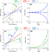 |
Fig. D.1 Evolution of the local power-law index (Γ) of a mass distribution. The influence of the mass transfer rate (ξ) and the fragmentation rate (ϕ) dependences with the mass M of the parental fragment is shown in (a), (b) and (c), (d) respectively. The solid lines, triangles and squares represent respectively the theoretical solutions from Eq. D.3, the Monte Carlo solutions obtained from a sample of 106 objects distributed in a power law of index Γ0 fragmenting according to Eq. D.8 and Eq. D.12. (a)-(c): Local power-law index (Γ) as a function of the initial slope Γ0 at scale R0/2. Dashed green and blue lines indicate the asymptotic limits of Γ(R). (b)-(d): Local power-law index (Γ) as a function of the spatial scale R for different initial slopes. The Monte Carlo solutions do not go below R/R0 ≈ 0.3 because the number of fragment constituting the fCMF becomes too large to compute. |
For smaller spatial scale R ≪ R0 the Monte Carlo simulation agrees with the theoretical prediction as Γ(R) converges to −1 if ∂ϕ/∂ log M < 0 (Fig. D.1d).
All Tables
All Figures
|
Fig. 1 Sketch of the hierarchical fragmentation model used. A parental object at spatial scale Rl (red) fragments into a number nl of children at scale Rl+1 (blue); here, nl = 2. The children are identified by an index i, where i = 1 represents the primary, (i.e. most massive) child. |
| In the text | |
|
Fig. 2 Parameter space for which a fCMF is compatible with the Maschberger (2013) cIMF in the sense of the AD test. Top: parameter space at which a fCMF is compatible with the cIMF at a 0.05 confidence level in the fragmentation rate (ϕ) versus mass transfer rate (ξ) diagram for the mass ratio (q) of different fragments. The yellow, blue, orange, green, red, and magenta patches highlight the solutions at Rstop = 741, 494, 329, 219, 146, 98 AU after l = 3, 4, 5, 6, 7, 8 levels of fragmentation, respectively. Crosses at q = 3.0 indicate points where the average total number of fragments produced at Rstop is ≈2.5. Bottom: fragmented CMF associated with the coloured labelled points. Dashed blue, red, and black lines represent the fCMF, cIMF, and the slope of the initial top-heavy CMF, respectively. The AD test is performed from M = 0.2 M⊙ to M = 150 M⊙ to compare the fCMF with the cIMF. |
| In the text | |
|
Fig. 3 Convergence of the local logarithmic slope Γ(R, M) under the influence of hierarchical fragmentation with the spatial scales R (solid black line) towards the Salpeter slope (dotted red line) for different initial slopes Γ0 = −2.0, −1.5, −0.5, 0, 0.5, 1.0. This convergence is only possible if |
| In the text | |
|
Fig. 4 Survival function of the fragmented CMF correlated with the multiplicity of stellar systems formed at different mass intervals. Top:104 random fragmentation draws (black lines) from the sample constituting the W43-MM2&MM3 CMF as presented in Pouteau et al. (2022, blue crosses) using the parameters ϕ = 1.0, ξ = −0.1, and q = 2. Fragmentation covers spatial scales from R0 = 2500 AU down to Rstop = 219 AU. For visibility, only the first 100 Monte Carlo draws are shown. The solid red and dashed blue line represents the cIMF and the power-law distribution fit from Pouteau et al. (2022) respectively. The dashed red line represents the average of the slopes obtained from fitting each Monte Carlo draw, using masses M > 0.8 M⊙. Bottom: distribution of the number of neighbours that a star of mass M possesses in different mass intervals (indicated above each plot). The mean value is indicated by the vertical dashed line. |
| In the text | |
|
Fig. 5 Multiplicity fraction as a function of the primary masses grouped inside bins for different fragmentation scenarios. Each Monte Carlo simulation was carried out using 104 random cores drawn from a top-heavy CMF with Γ = −0.95 (Pouteau et al. 2022), with ξ = −0.2, q = 2, and eight levels of fragmentation. Blue and black, and green and red dots respectively represent simulations using ϕ = 0.8, ϕ = 0.4, |
| In the text | |
|
Fig. B.1 Schematic view of the number of children of mass Ml+1 created at the scale Rl+1 (red dot) from one parental object of mass Ml at scale Rl (blue dot). In this work we assume that children result from the outcome of a single parental mass (solid coloured line) and neglect other possible contributions (crossed dotted lines). Since only the blue dot injects children in the red dot, the number of fragments inside the red dot corresponds to the number of parents inside the blue dot multiplied by the average number of fragments |
| In the text | |
|
Fig. C.1 Mass functions derived from our scale-free fragmentation model (blue), the Larson (1973) model (L73; red), and a Monte Carlo procedure (black). The mass functions are computed under the same condition as L73 with a pseudo-Dirac as a starting mass distribution centred at 103M⊙, 19 levels of fragmentation, mass transfer rate ξ = 0 and fragments mass ratio q = 1. At each level of fragmentation the objects subdivide into one or two fragments with respective probabilities 0.5 and 0.5. The different mass functions are multiplied by different constants to separate them for better visibility. |
| In the text | |
|
Fig. D.1 Evolution of the local power-law index (Γ) of a mass distribution. The influence of the mass transfer rate (ξ) and the fragmentation rate (ϕ) dependences with the mass M of the parental fragment is shown in (a), (b) and (c), (d) respectively. The solid lines, triangles and squares represent respectively the theoretical solutions from Eq. D.3, the Monte Carlo solutions obtained from a sample of 106 objects distributed in a power law of index Γ0 fragmenting according to Eq. D.8 and Eq. D.12. (a)-(c): Local power-law index (Γ) as a function of the initial slope Γ0 at scale R0/2. Dashed green and blue lines indicate the asymptotic limits of Γ(R). (b)-(d): Local power-law index (Γ) as a function of the spatial scale R for different initial slopes. The Monte Carlo solutions do not go below R/R0 ≈ 0.3 because the number of fragment constituting the fCMF becomes too large to compute. |
| In the text | |
Current usage metrics show cumulative count of Article Views (full-text article views including HTML views, PDF and ePub downloads, according to the available data) and Abstracts Views on Vision4Press platform.
Data correspond to usage on the plateform after 2015. The current usage metrics is available 48-96 hours after online publication and is updated daily on week days.
Initial download of the metrics may take a while.