| Issue |
A&A
Volume 709, May 2026
|
|
|---|---|---|
| Article Number | A77 | |
| Number of page(s) | 19 | |
| Section | Numerical methods and codes | |
| DOI | https://doi.org/10.1051/0004-6361/202556027 | |
| Published online | 05 May 2026 | |
FuGa3D: Fast full-sky analysis of Galaxy catalogues in 3D
1
University of Helsinki, Department of Physics,
PO Box 64,
00014
Helsinki,
Finland
2
Helsinki Institute of Physics,
PO Box 64,
00014
Helsinki,
Finland
3
Max-Planck-Institut für Astrophysik,
Karl-Schwarzschild-Str. 1,
85741
Garching,
Germany
4
Department of Astronomy, University of Geneva,
Ch. d’Ecogia 16,
1290
Versoix,
Switzerland
5
INAF – Osservatorio Astronomico di Roma,
via Frascati 33,
00040
Monteporzio Catone,
Italy
★ Corresponding author: This email address is being protected from spambots. You need JavaScript enabled to view it.
Received:
19
June
2025
Accepted:
16
January
2026
Abstract
We present FuGa3D, a code for fast computation of two-point statistics for galaxy-survey observables, including galaxy clustering and cosmic shear. We define the redshift–space correlation function (RCF) as the correlation function expressed in the parameter space of two redshifts and an angular separation angle. Assuming that there is no preferred direction in the sky, these parameters fully characterise the relative position of two galaxies independently of the assumed cosmological model. The conventional correlation metrics, such as the real-space clustering correlation function and its multipoles, can be constructed from the pre-computed RCF. The method provides a framework for efficient analysis of large cosmological datasets since the numerically expensive calculations only have to be carried out once and the subsequent cosmology-dependent analysis steps are cheap. We further define the redshift–space power spectrum as the harmonic counterpart of the RCF, and we show that it can be computed efficiently using the discrete galaxy coordinates. We validate the code with simulated mock catalogues, utilising a 40-core compute node. Computing the RCF and the real-space two-point correlation function up to the comoving 200 Mpc separation for a MICE simulation with 46 million galaxies at 1.5 Mpc (3 Mpc) resolution took 47 (12) node-minutes for clustering only and 7.3 (3.0) node-hours with shear analysis included.
Key words: gravitational lensing: weak / methods: data analysis / methods: statistical / galaxies: statistics / large-scale structure of Universe
© The Authors 2026
 Open Access article, published by EDP Sciences, under the terms of the Creative Commons Attribution License (https://creativecommons.org/licenses/by/4.0), which permits unrestricted use, distribution, and reproduction in any medium, provided the original work is properly cited.
This article is published in open access under the Subscribe to Open model. This email address is being protected from spambots. You need JavaScript enabled to view it. to support open access publication.
1 Introduction
Understanding the large-scale structure and the expansion history of the Universe is a key goal of modern cosmology. Two powerful observational techniques, galaxy clustering (GC) and weak gravitational lensing (WL), provide complementary probes of the distribution of matter in our Universe. Galaxy clustering measures the statistical distribution of galaxies. Weak lensing measures the subtle distortion of distant galaxy shapes due to gravitational deflection by intervening matter and offers a direct probe of the total mass distribution, independent of galaxy bias. Together, these methods allow for precise tests of cosmological models and constraints on the nature of dark energy.
The largest galaxy clustering surveys before the 2020s are provided by the 2dF Galaxy Reshift Survey (Colless et al. 2003) and Sloan Digital Sky Survey I-IV (York et al. 2000; Abazajian et al. 2009) and its various subprojects. The most recent observations come from Dark Energy Spectroscopic Instrument (DESI Collaboration 2025) and hint towards evolving dark energy. KiloDegree Survey (Heymans et al. 2021) performs a WL survey, and Dark Energy Survey (Dark Energy Survey Collaboration 2016) and Hyper Suprime-Cam (Li et al. 2023) combine clustering statistics with a WL survey.
The spectroscopic survey of the Euclid mission (Euclid Collaboration: Mellier et al. 2025) will measure the locations of tens of millions of galaxies at unprecedented accuracy. The photometric survey will image the WL effect on the shapes of over a billion galaxies. The Legacy Survey of Space and Time of Vera C. Rubin Observatory (Ivezić et al. 2019) is expected to provide a database of 20 billion galaxies. The Nancy Grace Roman Space Telescope (Akeson et al. 2019) is scheduled for launch in 2027. The analysis of these ever-increasing datasets calls for efficient analysis methods.
One of the fundamental tools used to quantify the clustering of galaxies is the two-point correlation function (2PCF; Peebles 1980), which measures the excess probability of finding galaxy pairs at a given separation compared to a random distribution. In addition to the simplest isotropic correlation function ξ(r), which is a function of the distance modulus r, anisotropic variants of the 2PCF can be defined to capture redshift–space distortion (RSD) effects that arise from the proper motion of galaxies or coherent flow of cosmic fluid (Kaiser 1987). Literature on RSD analyses is extensive. A few examples include the following: Peacock et al. (2001); Okumura et al. (2008); Guzzo et al. (2008); Beutler et al. (2012); Reid et al. (2012); Hou et al. (2018); Zarrouk et al. (2018); Bautista et al. (2021).
Constructing the real-space 2PCF requires knowledge of the geometry and the expansion history of the Universe. The radial distance to a galaxy cannot be measured directly. Instead, it must be inferred from the observed redshift. To convert the redshift into a distance, one has to assume a fiducial cosmological model and assign values to the cosmological parameters. Within the cosmological standard model, the Λ cold dark matter (ΛCDM) model, the matter density parameter (Ωm), vacuum energy density parameter (ΩΛ), and expansion rate (H0) in particular affect the redshift-distance relation. If the fiducial model differs from the true cosmology, the resulting 2PCF is distorted (Alcock & Paczynski 1979; Ballinger et al. 1996). It is possible to iterate the process with updated parameter values, but for modern large galaxy surveys, re-evaluating the 2PCF is a computationally heavy task. Standard methods to estimate the 2PCF, such as the Landy–Szalay (Landy & Szalay 1993) estimator, rely on counting galaxy pairs, a task whose computational complexity scales proportionally to the square of the number of galaxies, with survey volume fixed. Alternatively, if the distortion is small, one can apply a correction to the 2PCF to compensate for the difference between the fiducial model and the derived one.
Time evolution further complicates the analysis of the galaxy distribution in a deep survey. The conventional approach is to divide the survey into tomographic redshift shells and to treat each of them as a homogeneous sample at a fixed cosmological time. The shells should be narrow enough so that the time-evolution effects within a shell can be ignored but wide enough to include all scales of interest and to provide sufficient statistical power, which are somewhat contradictory requirements. Should one want to move from one tomographic binning scheme to another, the clustering 2PCF must be recomputed, which again is a computationally heavy process.
Weak lensing analysis does not rely on a fiducial model in the same way as clustering analysis. The WL approach is typically quantified in terms of the angular correlation function or angular spectrum of the shear field in tomographic redshift bins, which do not require converting redshifts to distances (e.g. Schneider et al. 2002; Kilbinger 2015). Nevertheless, WL studies often face the challenge of optimising tomographic binning. Once the shear field has been measured in a given binning configuration, re-running the entire analysis pipeline to adopt a different binning scheme can be computationally expensive. A method for re-binning the measured shear signal into alternative tomographic configurations – without requiring full recomputation of correlation functions or power spectra – would therefore be valuable.
The aim of this paper is twofold. First, we want to formulate a systematic model-independent description of the correlation structure in the observed galaxy distribution. In particular, we use the observed redshift z as a proxy for the radial distance. We define the redshift–space correlation function (RCF) and its harmonic counterpart, the redshift–space power spectrum (RP). The RCF can be regarded as a tomographic angular (cross-)correlation function at the limit of infinitesimally thin redshift shells. In a similar manner, the RP is the angular (auto and cross) power spectrum for infinitesimally thin tomographic bins. For a field with angular isotropy, the RCF contains all two-point correlation information, and any two-point statistical measure can be derived from it. Second, we introduce the Full-sky analysis of Galaxy catalogues in 3D (FuGa3D), a code for the fast analysis of galaxy catalogues. The methodology implemented in FuGa3D is based on the RCF and RP formalism. The main code constructs the RCF and RP data objects for very thin redshift shells, for galaxy clustering, weak lensing shear, and cross-correlation between the two. Once the primary data objects have been computed and stored on a disk, it is easy to re-bin them to form other two-point measures, such as the real-space correlation function for a given cosmological model, or the integrated angular correlation function or power spectrum for an arbitrary redshift range. The FuGa3D code package has a number of post-processing tools for this purpose. Using the provided tools, one can, for example, examine a space of cosmological models by converting the same input RCF into a real-space correlation function for different cosmological models.
The idea of using narrow redshift bins for model-independent clustering analysis is not new. Salazar-Albornoz et al. (2014) computed the angular correlation function w(θ) for narrow redshift bins on mock catalogues and studied the prospects of constraining the dark energy parameters without a fiducial model. Their work only utilised the autocorrelation.
This paper is structured as follows. In Sect. 2, we introduce the RCF and RP objects at the conceptual level, and we present the theoretical framework. The FuGa3D code is presented in the subsequent sections. The code offers two alternative ways of analysing galaxy catalogues: in configuration space or in harmonic space. We start by describing the configuration-space computation in Sect.3. In Sect.4, we extend the analysis to harmonic space. We show that the RP can be evaluated efficiently using discrete galaxy coordinates and that the RCF can be reconstructed from the RP. In Sect. 5, we validate the code using simulated galaxy mocks and demonstrate the usefulness of the RCF and RP formalism. We conclude and discuss future developments and applications in Sect. 6.
2 Correlation function and power spectrum in redshift space
2.1 Clustering correlation function
The conventional galaxy 2PCF is defined as the excess probability of finding two galaxies in volume elements dV1, dV2 at a separation distance of r, as compared to an unclustered distribution,
![Mathematical equation: $\[\mathrm{d} P\left(\boldsymbol{r}_0 ; \boldsymbol{r}_0+\boldsymbol{r}\right)=\bar{n}_1 \bar{n}_2[1+\xi(\boldsymbol{r})] \mathrm{d} V_1 \mathrm{~d} V_2,\]$](/articles/aa/full_html/2026/05/aa56027-25/aa56027-25-eq1.png) (1)
(1)
where ![Mathematical equation: $\[\bar{n}_{1}, \bar{n}_{2}\]$](/articles/aa/full_html/2026/05/aa56027-25/aa56027-25-eq2.png) is the average density of observable galaxies at the two locations, and ξ(r) defines the correlation function. The expression assumes statistical homogeneity; the correlation function depends only on the relative distance r.
is the average density of observable galaxies at the two locations, and ξ(r) defines the correlation function. The expression assumes statistical homogeneity; the correlation function depends only on the relative distance r.
In a statistically homogeneous and isotropic universe, ξ(r) would be a function of the modulus of r. We could ignore the orientation of the galaxy pair and write ξ(r) = ξ(r). The RSDs complicate the picture. The anisotropy of the correlation structure is captured by the two-dimensional correlation function ξ(r, μ), where μ is the cosine of the angle between the local line-of-sight (LOS) and the line connecting two galaxies. It is convenient to expand this in Legendre polynomials as
![Mathematical equation: $\[\xi(r, \mu)=\sum_{\ell} \xi_{\ell}(r) L_{\ell}(\mu).\]$](/articles/aa/full_html/2026/05/aa56027-25/aa56027-25-eq3.png) (2)
(2)
This defines the correlation function multipoles ξℓ(r). In the absence of anisotropy, only the monopole ξ0(r) differs from zero. The expansion is not unique and depends on the definition of the local LOS.
Even the correlation function of Eq. (1) is not fully general. It assumes statistical homogeneity, that the density of objects and the correlation function are equal everywhere in space. While this may be true at a fixed cosmological time, it does not hold for an observed light cone, which is a combination of galaxies at different distances and thus at different stages of their evolution. The correlation function evolves over time, making the observed correlation a function of distance.
We now drop the assumption of statistical homogeneity but keep the assumption of angular isotropy: the correlation function will depend on the angular distance between the two galaxies, but it remains unchanged if the pair is rotated to another orientation, or transported to another position on the sky. In other words, there is no preferred direction or orientation in the sky. We define the RCF ξ(z1, z2, θ) for clustering as the excess probability of finding two galaxies at redshifts z1 and z2, and separated by angular distance θ. Let Ω denote a direction on the sky, specified by the spherical coordinates {ϑ, φ}, or by RA and Dec. The position of a galaxy in redshift space is fully defined by the coordinates {z, Ω}. The probability of finding two galaxies at positions {z1, Ω1}, {z2, Ω2} can be written as
![Mathematical equation: $\[\mathrm{d} P\left(z_1, \Omega_1 ; z_2, \Omega_2\right)=\bar{n}_1 \bar{n}_2\left(1+\xi\left(z_1, z_2, \theta\right)\right) \mathrm{d} V_1 \mathrm{~d} V_2,\]$](/articles/aa/full_html/2026/05/aa56027-25/aa56027-25-eq4.png) (3)
(3)
where θ is the angular distance between directions Ω1 and Ω2, and ![Mathematical equation: $\[\bar{n}_{1}, \bar{n}_{2}\]$](/articles/aa/full_html/2026/05/aa56027-25/aa56027-25-eq5.png) represent the unclustered density. We write it separately for locations 1 and 2, to accommodate a distance-dependent selection function (the fainter the object, the closer it must be to be observable), or position-dependent selection effects.
represent the unclustered density. We write it separately for locations 1 and 2, to accommodate a distance-dependent selection function (the fainter the object, the closer it must be to be observable), or position-dependent selection effects.
We cannot do a similar reduction of variables in the radial dimension. The same separation in redshift corresponds to a different physical distance depending on the redshift; thus we cannot reduce the redshift dimension without assuming a cosmological model, which is exactly what we want to avoid. The RCF is necessarily a function of two redshifts.
The RCF can be interpreted as the tomographic angular correlation function for infinitesimally thin redshift shells. Under the assumption of angular isotropy, the RCF contains all information on the correlation structure of the galaxy sample, in a form that is independent of an assumed cosmological model, or of time evolution. It is also independent of the definition of the LOS.
Alternatively, the clustering correlation function can be defined through the relative density fluctuation
![Mathematical equation: $\[\delta(z, \Omega)=\frac{n(z, \Omega)}{\langle n(z, \Omega)\rangle}-1,\]$](/articles/aa/full_html/2026/05/aa56027-25/aa56027-25-eq6.png) (4)
(4)
where n(z, Ω) is the observed galaxy density, and ⟨n(z, Ω)⟩ represents the mean density at the same location. We write it as a function of the spatial coordinates z, Ω, to allow for location-dependent selection effects. The brackets denote an ensemble average. The local galaxy density is thought to represent a random deviation around the mean value. By definition ⟨δ⟩ = 0. The RCF is then defined as
![Mathematical equation: $\[\xi\left(z_1, z_2, \theta\right)=\left\langle\delta\left(z_1, \Omega_1\right) \delta\left(z_2, \Omega_2\right)\right\rangle.\]$](/articles/aa/full_html/2026/05/aa56027-25/aa56027-25-eq7.png) (5)
(5)
With ![Mathematical equation: $\[\bar{n}\]$](/articles/aa/full_html/2026/05/aa56027-25/aa56027-25-eq8.png) identified with ⟨n⟩, the definition of Eq. (5) is equivalent to that of Eq. (3). When viewed at very fine resolution, the galaxy density n becomes a collection of delta peaks. Consequently, δ becomes a function that takes a negative value everywhere except at the locations of observed galaxies, where it is infinite (the correlation of Eq. (5) is still finite). This makes the definition of Eq. (3) possibly more intuitive, but mathematically the two definitions are equivalent. We make use of Eq. (4) when constructing the cross-correlation between the shear field and galaxy density.
identified with ⟨n⟩, the definition of Eq. (5) is equivalent to that of Eq. (3). When viewed at very fine resolution, the galaxy density n becomes a collection of delta peaks. Consequently, δ becomes a function that takes a negative value everywhere except at the locations of observed galaxies, where it is infinite (the correlation of Eq. (5) is still finite). This makes the definition of Eq. (3) possibly more intuitive, but mathematically the two definitions are equivalent. We make use of Eq. (4) when constructing the cross-correlation between the shear field and galaxy density.
The conventional two-point correlation measures of the galaxy distribution can be written in terms of the RCF. For instance, one can
average over z1, z2 to yield the angular correlation function for an arbitrary redshift range,
adopt a cosmological model to convert redshifts to physical distances and to rebin the correlation function to the real-space 2PCF.
2.2 Shear correlation function
In a similar manner we define the RCF for the shear field γ as a function of two redshifts and an angular separation as
![Mathematical equation: $\[\begin{aligned}\xi_{\mathrm{tt}}\left(z_1, z_2, \theta\right) & =\left\langle\gamma_{\mathrm{t}}\left(z_1, \Omega_1\right) \gamma_{\mathrm{t}}\left(z_2, \Omega_2\right)\right\rangle, \\\xi_{\times \times}\left(z_1, z_2, \theta\right) & =\left\langle\gamma_{\times}\left(z_1, \Omega_1\right) \gamma_{\times}\left(z_2, \Omega_2\right)\right\rangle,\end{aligned}\]$](/articles/aa/full_html/2026/05/aa56027-25/aa56027-25-eq9.png) (6)
(6)
where γt and γ× are the tangential and cross shear components, defined with respect to the great circle connecting Ω1 and Ω2.
It is customary to write the correlation function as ‘plus’ and ‘minus’ components:
![Mathematical equation: $\[\begin{aligned}& \xi_{+}\left(z_1, z_2, \theta\right)=\xi_{\mathrm{tt}}\left(z_1, z_2, \theta\right)+\xi_{\times \times}\left(z_1, z_2, \theta\right) ,\\& \xi_{-}\left(z_1, z_2, \theta\right)=\xi_{\mathrm{tt}}\left(z_1, z_2, \theta\right)-\xi_{\times \times}\left(z_1, z_2, \theta\right).\end{aligned}\]$](/articles/aa/full_html/2026/05/aa56027-25/aa56027-25-eq10.png) (7)
(7)
In the same way, one can define cross-correlation components ξt×, ξ×t. However, these are usually expected to vanish on grounds of parity symmetry.
To define the cross-correlation function between density and shear, we made use of Eq. (4). The cross-correlation between density and tangential shear becomes
![Mathematical equation: $\[\xi_{\mathrm{ct}}\left(z_1, z_2, \theta\right)=\left\langle\delta\left(z_1, \Omega_1\right) \gamma_{\mathrm{t}}\left(z_2, \Omega_2\right)\right\rangle.\]$](/articles/aa/full_html/2026/05/aa56027-25/aa56027-25-eq11.png) (8)
(8)
Again, based on parity symmetry, the component ξc× is expected to vanish.
The following symmetry relations should be obvious:
![Mathematical equation: $\[\begin{aligned}\xi_{\mathrm{cc}}(z_1, z_2, \theta) & =\xi_{\mathrm{cc}}(z_2, z_1, \theta), \\\xi_{+}(z_1, z_2, \theta) & =\xi_{+}(z_2, z_1, \theta), \\\xi_{-}(z_1, z_2, \theta) & =\xi_{-}(z_2, z_1, \theta), \\\xi_{\mathrm{ct}}(z_1, z_2, \theta) & =\xi_{\mathrm{tc}}(z_2, z_1, \theta).\end{aligned}\]$](/articles/aa/full_html/2026/05/aa56027-25/aa56027-25-eq12.png) (9)
(9)
Similar relations hold for other auto-correlation and cross-correlation components. Here we used the subscript cc to denote the clustering correlation.
2.3 Redshift-space power spectrum
We further define the redshift–space (angular) power spectra (RP) ![Mathematical equation: $\[P_{\ell}^{X Y}(z_{1}, z_{2})\]$](/articles/aa/full_html/2026/05/aa56027-25/aa56027-25-eq13.png) , where X, Y = C, E, B, as the harmonic-space counterparts of the RCF components. Here, C refers to the density fluctuation. The T, × components of the shear field have a correspondence in the E, B components in harmonic space. The relations between the non-vanishing components of RCF and RP are given by
, where X, Y = C, E, B, as the harmonic-space counterparts of the RCF components. Here, C refers to the density fluctuation. The T, × components of the shear field have a correspondence in the E, B components in harmonic space. The relations between the non-vanishing components of RCF and RP are given by
![Mathematical equation: $\[\begin{aligned}& \xi_{\mathrm{cc}}(z_1, z_2, \theta)=\sum_{\ell} \frac{2 \ell+1}{4 \pi} C_{\ell}^{C C}(z_1, z_2) d_{00}^{\ell}(\theta),\\& \xi_{+}(z_1, z_2, \theta)=\sum_{\ell} \frac{2 \ell+1}{4 \pi}[C_{\ell}^{E E}(z_1, z_2)+C_{\ell}^{B B}(z_1, z_2)] d_{2,2}^{\ell}(\theta),\\& \xi_{-}(z_1, z_2, \theta)=\sum_{\ell} \frac{2 \ell+1}{4 \pi}[C_{\ell}^{E E}(z_1, z_2)-C_{\ell}^{B B}(z_1, z_2)] d_{2,-2}^{\ell}(\theta),\\& \xi_{\mathrm{ct}}(z_1, z_2, \theta)=-\sum_{\ell} \frac{2 \ell+1}{4 \pi} C_{\ell}^{C E}(z_1, z_2) d_{20}^{\ell}(\theta),\end{aligned}\]$](/articles/aa/full_html/2026/05/aa56027-25/aa56027-25-eq14.png) (10)
(10)
where ![Mathematical equation: $\[d_{s s^{\prime}}^{\ell}(\theta)\]$](/articles/aa/full_html/2026/05/aa56027-25/aa56027-25-eq15.png) are the reduced Wigner functions (see, e.g. Varshalovich et al. 1988). The derivation of these results and their inverse relations, including the zero components, is given in Appendix A.
are the reduced Wigner functions (see, e.g. Varshalovich et al. 1988). The derivation of these results and their inverse relations, including the zero components, is given in Appendix A.
3 Computation on sphere
3.1 FuGa3D
We now proceed to describe the FuGa3D analysis code. The code implements an efficient computation of the RCF and RP data objects from a given galaxy catalogue, and contains tools for their further analysis. The main code takes as input a galaxy catalogue. In the catalogue, each galaxy is described by its location on the celestial sphere (RA, Dec), redshift, and, optionally, the shear components γ1, γ2. From these inputs, FuGa3D constructs a number of output products. The primary outputs are the RCF ξX(z1, z2, θ), the integrated angular correlation function ξX(θ) for the full redshift range, the RP PYℓ(z1, z2), and the integrated angular power spectrum PYℓ. The subscripts X, Y refer to the components of galaxy density and shear. While the true RCF and RP are continuous functions of two redshifts, their data-derived estimates involve a binning scheme in z (and in θ in the case of the RCF). Input parameters set the redshift range and resolution, as well as the range and resolution in θ.
Further derived data products can be constructed with auxiliary tools: The real-space 2PCF of the galaxy density is constructed from the RCF with the Realspace tool, given a cosmological model. Auxiliary tools also allow for integrating of the RCF or RP objects to yield an angular correlation function or power spectrum for an arbitrary redshift range. The Spectrum tool corrects the raw RP for the effects of the sky mask, and, optionally, performs conversion from harmonic space to configuration space. There are thus two complementary ways of constructing the RCF, both with their benefits and caveats: 1. direct map-based computation based on pair counting, and 2. power-spectrum estimation involving a spherical harmonic transform (SHT), followed by a mask correction and a transformation to configuration space. While the direct approach is conceptually simpler, it involves a limitation: For the computation of the clustering correlation, FuGa3D implements a variant of the Landy–Szalay (hereafter LS) estimator with a highly efficient speed-up algorithm, which however relies on some geometric simplifications. In particular, we assume a piecewise uniform selection function and a cone-like geometry. This may limit the usefulness of the method if the actual selection function contains strong small-scale structure. This approximation does not concern the SHT approach. The latter, on the other hand, involves the demanding additional step of correcting for the sky mask.
We begin by describing the direct RCF computation, as implemented in FuGa3D. The harmonic-space computation is described in Sect. 4.
3.2 Resolution and storage
The FuGa3D code operates on a 3D grid which combines uniformly spaced redshift shells with Healpix (Górski et al. 2005) pixels. The redshift resolution is set by the user-defined parameter z_delta. The same resolution parameter also sets the redshift resolution of the output RCF and RP objects.
In the current implementation, we have assumed perfect redshift information. Each galaxy is placed in a single redshift shell according to the observed redshift read from the input catalogue.
The code makes use of a hierarchical pixelization scheme which involves two distinct Healpix resolutions: The sky is first divided into low-resolution pixels, at a resolution determined by parameter nside_base. For instance, nside_base=32 divides the sky into 12 288 pixels of 3.35 deg2 each. We refer to these low-resolution pixels as base pixels. The base pixels serve several purposes, including bookkeeping and handling the radial selection function. Each low-resolution pixel is further divided into smaller pixels at nside_high resolution. The correlation functions are computed at this high resolution. Moving back and forth between the two resolutions is straightforward in the NESTED pixel ordering scheme of Healpix.
Due to the discretisation, we lose information on scales smaller than the pixel size. The error can be reduced by increasing the resolution, at the price of increasing computational cost. There is thus a trade-off involved. The results in this work have been obtained with resolutions in the range nside_high=512–2048 and z_delta=0.0005–0.005.
The computation of the galaxy correlation function requires knowledge of the selection function S(z, Ω). The selection function tells which fraction of all galaxies is observable at a given location. In our implementation, the selection function is assumed to be isotropic within one base pixel, that is, a function of redshift only. This assumption is crucial for the speed-up algorithm implemented in FuGa3D, as we explain shortly. The selection function can either be estimated from the data catalogue itself or be provided in the form of an external random catalogue.
From the requirement of the isotropic selection function, it follows that the survey boundary is not allowed to pass through a base pixel. In the first processing step, the data catalogue is trimmed at the survey boundaries to match the low-resolution pixelisation. Partially filled pixels are removed from further processing. This is achieved through the following procedure. We examine the distribution of galaxies per base pixel, ignoring the redshift. We identify all low-resolution pixels that have empty pixels as neighbours (Fig. 1). We interpret these pixels as being partially filled, and we discard the galaxies in them. As a result, we have a binary survey mask consisting of base pixels that are either empty or fully covered. Keeping track of the survey mask is now simple: we only need to keep track of which base pixels are included in the survey.
Discarding the galaxies at the survey edges means that we lose part of the information in the galaxy catalogue. In practice, the data loss is small and has little effect on the results. The data loss can be reduced by increasing the base resolution, but a very high base resolution leads to inefficient data handling.
The data stored in memory consists of the number of galaxies in each cell of the 3D grid, and their co-added shear (if available). In a typical situation, the grid is sparse, and a majority of the cells are empty. The data is stored in a memory-efficient way, as follows. For each base pixel under the mask, the code stores an array object of fixed length, whose elements are in turn arrays of flexible length. The first dimension corresponds to high-resolution pixels within the base pixel. For each of those high-resolution pixels, the code stores an array of indices pointing to the redshift bins that contain a galaxy (or several). Other data objects of the same structure hold the number of galaxies and the co-added shear for the same cells. This data storage scheme ensures efficient use of memory, as empty cells do not consume memory.
The hierarchical pixelisation offers flexibility in handling different survey footprints. With the same code and with the same data structures we can store a full-sky survey at modest pixel resolution, or a small survey with a very high resolution.
 |
Fig. 1 Trimming of survey edges. Partially filled base pixels are discarded from analysis to ensure uniform coverage over the full survey area. Empty base pixels are marked by red crosses. Pixels with an empty pixel as a neighbour, either directly (blue) or diagonally (purple), are interpreted as being on the survey boundary. Both the empty pixels and their neighbours are discarded from further analysis. |
3.3 Clustering correlation function
The standard way of estimating the correlation between two galaxy locations is with the LS estimator
![Mathematical equation: $\[\xi(z_1, z_2, \theta)=\frac{d d(z_1, z_2, \theta)-d r(z_1, z_2, \theta)-r d(z_1, z_2, \theta)}{r r(z_1, z_2, \theta)}+1,\]$](/articles/aa/full_html/2026/05/aa56027-25/aa56027-25-eq16.png) (11)
(11)
where dd, dr, rd, rr are normalised pair counts: galaxy–galaxy, galaxy–random, random–galaxy, and random–random pairs in discrete parameter bins. The estimator requires a random catalogue that represents an uncorrelated distribution with the same selection function and boundary effects as the actual data catalogue. The counts are normalised to the total number of pairs. The cross-count dr is not symmetric with respect to exchange dr ↔ rd (a galaxy at low z, and a random point at high z, is not the same thing as a galaxy at high z, and a random point at low z). The correlation function must therefore count both.
We apply to correlation function estimation a method that mimics the LS estimator at the limit of an infinite random catalogue. Consider one cell of our 3D grid at redshift z and in angular direction Ω. The cell combines a Healpix pixel with a small redshift interval. We denote the expected number of observed galaxies in the cell by α(z, Ω). It can be written as
![Mathematical equation: $\[\alpha(z, \Omega)=\bar{n}_{\mathrm{tot}}(z) S(z, \Omega) \Delta V(z),\]$](/articles/aa/full_html/2026/05/aa56027-25/aa56027-25-eq17.png) (12)
(12)
where ![Mathematical equation: $\[\bar{n}_{\text {tot}}(z)\]$](/articles/aa/full_html/2026/05/aa56027-25/aa56027-25-eq18.png) is the mean galaxy density at redshift z, a function of z to allow for time-evolution effects. The density of observable galaxies is
is the mean galaxy density at redshift z, a function of z to allow for time-evolution effects. The density of observable galaxies is ![Mathematical equation: $\[\bar{n}=S(z, \Omega) \bar{n}_{\text {tot}}\]$](/articles/aa/full_html/2026/05/aa56027-25/aa56027-25-eq19.png) , where S(z, Ω) is the position-dependent selection function, and ΔV(z) is the volume of the grid cell. Since Healpix pixels have equal areas, the volume of the cell is proportional to the radial diameter of the cell. For a given z bin it depends on the cosmology and thus is not known a priori. Nor do we know the mean density or the selection function independently. What we need, however, is not the individual factors, but the combination of Eq. (12), and this we can estimate from the data, assuming that the selection function is either isotropic over the mask area, or a slowly varying function of Ω. It is obtained from the average number of galaxies per pixel in the redshift shell and the area in question. Obviously, the average must be taken over a sufficiently large area to smooth out local fluctuations. By default, FuGa3D estimates α from the input galaxy catalogue. Alternatively, if external information on the mean density is available, this additional information can be injected in the form of a random catalogue, which FuGa3D then converts into an estimate for α.
, where S(z, Ω) is the position-dependent selection function, and ΔV(z) is the volume of the grid cell. Since Healpix pixels have equal areas, the volume of the cell is proportional to the radial diameter of the cell. For a given z bin it depends on the cosmology and thus is not known a priori. Nor do we know the mean density or the selection function independently. What we need, however, is not the individual factors, but the combination of Eq. (12), and this we can estimate from the data, assuming that the selection function is either isotropic over the mask area, or a slowly varying function of Ω. It is obtained from the average number of galaxies per pixel in the redshift shell and the area in question. Obviously, the average must be taken over a sufficiently large area to smooth out local fluctuations. By default, FuGa3D estimates α from the input galaxy catalogue. Alternatively, if external information on the mean density is available, this additional information can be injected in the form of a random catalogue, which FuGa3D then converts into an estimate for α.
From here on we assume that α(z, Ω) is known. We denote by α(zk, Ωij) its value on the kth redshift shell and in Healpix pixel Ωij. We introduce here a double-index notation where the first index i refers to a base pixel, and the second index j labels high-resolution pixels inside it. The motivation for the double indexing scheme will become clear in due course. Similarly, we denote by n(zk, Ωij) the actual number of galaxies in the same cell. Due to the chosen normalisation,
![Mathematical equation: $\[\sum_{i j k} \alpha(z_k, \Omega_{i j})=\sum_{i j k} n(z_k, \Omega_{i j})=N,\]$](/articles/aa/full_html/2026/05/aa56027-25/aa56027-25-eq20.png) (13)
(13)
where N is the total number of galaxies in the sample. The quantity α(Ωij, zk) represents the number of galaxies in a 3D cell, if the galaxies were uniformly distributed, and takes the role of the random catalogue in the LS estimator.
The true RCF, as defined through Eq. (3), is a continuous function of its parameters. When it is estimated from data, the parameter space must be divided into discrete bins (just as with the usual 2PCF). We divide the range of interest in θ into Nθ bins, and label them as θm, m = 1 . . . Nθ. In redshift, we adopt the bin structure from the 3D space, that is, spacing at resolution z_delta. In the following, a cell refers to an element of the spherical 3D grid, specified by coordinates {z, Ω}, while a bin refers to an element in the parameter space of {z1, z2, θ}.
We need three data objects that correspond to the pair counts dd, dr, rr of the LS estimator. They are data objects of the same size and form as the RCF itself, that is, defined in the coordinate space {z1, z2, θ}. In the following, we consider each of the objects dd, dr, rr in turn. We start from dd, which is constructed as
![Mathematical equation: $\[\begin{aligned}& d d(z_k, z_{k^{\prime}}, \theta_m)= \\& \frac{1}{N(N-1)} \sum_{i i^{\prime} \in S} \sum_{j j^{\prime}} \Theta(\Omega_{i j}-\Omega_{i^{\prime} j^{\prime}} \in \theta_m) n(z_k, \Omega_{i j}) n(z_{k^{\prime}}, \Omega_{i^{\prime} j^{\prime}}),\end{aligned}\]$](/articles/aa/full_html/2026/05/aa56027-25/aa56027-25-eq21.png) (14)
(14)
where ii′ ∈ S indicates that we include in the first sum only the base pixels inside the survey area, and Θ(Ωij − Ωi′j′ ∈ θm) has the role of assigning the pairs into the respective θ bins. Specifically, Θ(Ωij − Ωi′j′ ∈ θm) = 1 if the angular distance between the centres of pixels Ωij and Ωi′j′ falls in bin θm, and it vanishes otherwise. As implied by the prefactor 1/[N(N − 1)], we do not count pairs where both components are the same galaxy. Thus, in the special case where i = i′, j = j′, k = k′, the term inside the sum should read n(zk, Ωij)[n(zk, Ωij) − 1], and this is assigned to the lowest θ bin. For clarity of expression, we do not write this separately in Eq. (14).
The ordering of the elements in Eq. (14) reflects the loop structure of the code. Evaluating the expression of Eq. (14) algorithmically involves six nested loops, with the four outer-most loops corresponding to the sums in Eq. (14), and the two innermost ones to the redshift bins. Let Nbase be the number of pixels at base resolution, Nsub = the number of high-resolution pixels included in one base-resolution pixel, and Nzbin the number of redshift shells. For example, with nside_base=32 and nside_high=1024 we have Nbase = 12 · 322 = 12 288, and Nsub = (1024/32)2 = 1024. Naively, the computational complexity of the evaluation would be ![Mathematical equation: $\[N_{\text {base}}^{2} \times N_{\text {sub}}^{2} \times N_{\text {zbin}}^{2}\]$](/articles/aa/full_html/2026/05/aa56027-25/aa56027-25-eq22.png) . In reality, it is much less than that. The first two loops(i, i′ ∈ S) scan through pairs of base pixels within the survey mask. Usually, one is interested in a limited angular range θ < θmax. Base pixel pairs far outside the range of interest can be discarded immediately (the Healpix package includes routines for this). The actual number of base pixel pairs that require closer inspection is typically of the order of Npairs ~ 10 000 − 100 000 rather than
. In reality, it is much less than that. The first two loops(i, i′ ∈ S) scan through pairs of base pixels within the survey mask. Usually, one is interested in a limited angular range θ < θmax. Base pixel pairs far outside the range of interest can be discarded immediately (the Healpix package includes routines for this). The actual number of base pixel pairs that require closer inspection is typically of the order of Npairs ~ 10 000 − 100 000 rather than ![Mathematical equation: $\[N_{\text {base}}^{2}\]$](/articles/aa/full_html/2026/05/aa56027-25/aa56027-25-eq23.png) . Thus, the two-level scheme works not only as a means for bookkeeping but also as an efficient preselector in correlation-function estimation. The next two loops (j, j′) scan through high-resolution pixel pairs between the base pixel pair (i, i′). Most of the computation time is taken by the evaluation of the angular distance θ between the pixel pair. This does not depend on redshift and only needs to be done once for a pixel pair. The two innermost loops scan over the redshift bins (k, k′) and accumulate the products n(zk, Ωij n(zk′, Ωi′j′) in the respective bins of the dd grid. In a typical case, most redshift cells are empty. For instance, with nside_high=1024 and Nzbin = 1000 redshift bins we have over 1010 grid cells, while a typical galaxy catalogue has a few million objects. It is thus inevitable that a vast majority of the cells are empty (and those that are not, mostly contain just one galaxy). Since only the non-empty grid cells are stored in memory, the last (k, k′) loops only need to scan through a couple of elements. In total, the computational complexity of the evaluation of the dd array is of the order of
. Thus, the two-level scheme works not only as a means for bookkeeping but also as an efficient preselector in correlation-function estimation. The next two loops (j, j′) scan through high-resolution pixel pairs between the base pixel pair (i, i′). Most of the computation time is taken by the evaluation of the angular distance θ between the pixel pair. This does not depend on redshift and only needs to be done once for a pixel pair. The two innermost loops scan over the redshift bins (k, k′) and accumulate the products n(zk, Ωij n(zk′, Ωi′j′) in the respective bins of the dd grid. In a typical case, most redshift cells are empty. For instance, with nside_high=1024 and Nzbin = 1000 redshift bins we have over 1010 grid cells, while a typical galaxy catalogue has a few million objects. It is thus inevitable that a vast majority of the cells are empty (and those that are not, mostly contain just one galaxy). Since only the non-empty grid cells are stored in memory, the last (k, k′) loops only need to scan through a couple of elements. In total, the computational complexity of the evaluation of the dd array is of the order of ![Mathematical equation: $\[N_{\text {pairs}} \times N_{\text {sub}}^{2} \times\]$](/articles/aa/full_html/2026/05/aa56027-25/aa56027-25-eq24.png) (a few).
(a few).
We examine the evaluation of rr, which represents random-random pair counts. We do not have an explicit random catalogue; its role is taken by the factor α, which incorporates our knowledge of the survey geometry and of the selection function. Imagine that we had a very large random catalogue with MN objects, and M → ∞. The number of random points in a cell approaches Mα(zk, Ωij), and the normalised rr count is obtained as
![Mathematical equation: $\[\begin{aligned}& r r(z_k, z_{k^{\prime}}, \theta_m)=\frac{1}{M N(M N-1)} \\& \sum_{i j} \sum_{i^{\prime} j^{\prime}} \Theta(\Omega_{i j}-\Omega_{i^{\prime} j^{\prime}} \in \theta_m) M \alpha(z_k, \Omega_{i j}) M \alpha(z_{k^{\prime}}, \Omega_{i^{\prime} j^{\prime}}) \\& \quad arrow \frac{1}{N^2} \sum_{i j} \sum_{i^{\prime} j^{\prime}} \Theta(\Omega_{i j}-\Omega_{i^{\prime} j^{\prime}} \in \theta_m) \alpha(z_k, \Omega_{i j}) \alpha(z_{k^{\prime}}, \Omega_{i^{\prime} j^{\prime}}).\end{aligned}\]$](/articles/aa/full_html/2026/05/aa56027-25/aa56027-25-eq25.png) (15)
(15)
This is similar to the expression for dd, with the difference that instead of n we have α, which, unlike n, is not sparse. Thus, the evaluation with the dd algorithm would be much more expensive. This is where the assumption of an isotropic selection function steps in. In the simplest case, the selection function can be assumed to be isotropic over the survey area, that is, it depends only on z. The isotropy of the selection function implies an isotropic survey depth: the survey shape is a cone, with equal depth in all directions within the survey area. We can then write α(zk, Ωij) = α(zk)m(Ωi), where m(Ωi) is a binary survey mask, with m(Ωi) = 1 when the base pixel is inside the survey area and m(Ωi) = 0 when the pixel is outside. Recall that our survey area has been trimmed to consist of full base pixels; therefore, the mask only depends on the index i. The sum can now be rearranged to
![Mathematical equation: $\[r r(z_k, z_{k^{\prime}}, \theta_m)=\frac{1}{N^2} \alpha(z_k) \alpha(z_{k^{\prime}}) \sum_{i i^{\prime} \in S} \sum_{j j^{\prime}} \Theta(\Omega_{i j}-\Omega_{i^{\prime} j^{\prime}} \in \theta_m).\]$](/articles/aa/full_html/2026/05/aa56027-25/aa56027-25-eq26.png) (16)
(16)
The four sums simply count the number of pixel pairs with angular distance inside bin θm. The computational complexity of this operation is ![Mathematical equation: $\[N_{\text {pairs}} \times N_{\text {sub}}^{2}\]$](/articles/aa/full_html/2026/05/aa56027-25/aa56027-25-eq27.png) , and the result is a small array of length Nθ. Scaling it by α(zk) and α(zk′) and spreading it on the rr grid is a very fast process.
, and the result is a small array of length Nθ. Scaling it by α(zk) and α(zk′) and spreading it on the rr grid is a very fast process.
In a somewhat more complicated scheme, we relax the assumption of isotropy over the survey area and require isotropy only within a base pixel. We can now write α(zk, Ωij ) = α(zk, Ωi). The expression for rr becomes
![Mathematical equation: $\[\begin{aligned}& rr(z_k, z_{k^{\prime}}, \theta_m)= \\& \quad \frac{1}{N^2} \sum_{i i^{\prime} \in S} \alpha(z_k, \Omega_i) \alpha(z_{k^{\prime}}, \Omega_{i^{\prime}}) \sum_{j j^{\prime}} \Theta(\Omega_{i j}-\Omega_{i^{\prime} j^{\prime}} \in \theta_m).\end{aligned}\]$](/articles/aa/full_html/2026/05/aa56027-25/aa56027-25-eq28.png) (17)
(17)
The procedure of counting pixel pairs, scaling by α, and spreading on the target grid, is now repeated for each pair of base pixels ii′. This is computationally more expensive than the fully isotropic case, but still significantly less expensive than brute-force computation with an arbitrary selection function.
The third element in the correlation function estimation is dr, which represents cross-pair counts between the data catalogue and the random catalogue. Combining the characteristics of dd and rr estimation, we find
![Mathematical equation: $\[\begin{aligned}& d r(z_k, z_{k^{\prime}}, \theta_m)= \\& \quad \frac{1}{N^2} \alpha(z_{k^{\prime}}) \sum_{i i^{\prime} \in S} \sum_j n(z_k, \Omega_{i j}) \sum_{j^{\prime}} \Theta(\Omega_{i j}-\Omega_{i^{\prime} j^{\prime}} \in \theta_m)\end{aligned}\]$](/articles/aa/full_html/2026/05/aa56027-25/aa56027-25-eq29.png) (18)
(18)
for the isotropic case and
![Mathematical equation: $\[\begin{aligned}& d r(z_k, z_{k^{\prime}}, \theta_m)= \\& \quad \frac{1}{N^2} \sum_{i i^{\prime} \in S} \alpha(z_{k^{\prime}}, \Omega_{i^{\prime}}) \sum_j n(z_k, \Omega_{i j}) \sum_{j^{\prime}} \Theta(\Omega_{i j}-\Omega_{i^{\prime} j^{\prime}} \in \theta_m)\end{aligned}\]$](/articles/aa/full_html/2026/05/aa56027-25/aa56027-25-eq30.png) (19)
(19)
for the pixelwise isotropic case. The sum over j′ counts pixels within distance θm from pixel Ωij. This is multiplied by the galaxy counts in the first pixel, accumulated in an array of size (Nzbin, Nθ), and finally distributed on the dr grid.
The final correlation function is constructed as
![Mathematical equation: $\[\begin{aligned}& \hat{\xi}(z_k, z_{k^{\prime}}, \theta_m)= \\& \quad \frac{d d(z_k, z_{k^{\prime}}, \theta_m)-d r(z_k, z_{k^{\prime}}, \theta_m)-r d(z_k, z_{k^{\prime}}, \theta_m)}{r r(z_k, z_{k^{\prime}}, \theta_m)}+1,\end{aligned}\]$](/articles/aa/full_html/2026/05/aa56027-25/aa56027-25-eq31.png) (20)
(20)
where
![Mathematical equation: $\[r d(z_k, z_{k^{\prime}}, \theta_m)=d r(z_{k^{\prime}}, z_k, \theta_m).\]$](/articles/aa/full_html/2026/05/aa56027-25/aa56027-25-eq32.png) (21)
(21)
When computing the components of the correlation function, we exploit the symmetry with respect to the exchange ijk ↔ i′j′k′ to speed up the computation. The loops run through half of the index space, and we update two elements of the target array at one step.
3.4 Shear correlation function
Computing the shear correlation function is rather straightforward compared with computing the clustering correlation. To start, the measured ellipticity of a galaxy is interpreted as a direct measure of the shear field γ at the location of the galaxy. The shear of a 3D cell, γijk, is taken to be the average of all galaxy ellipticities in that cell,
![Mathematical equation: $\[\gamma_{i j k} \equiv \gamma(z_k, \Omega_{i j})= \begin{cases}n(z_k, \Omega_{i j})^{-1} \sum_m \epsilon_m, & n(z_k, \Omega_{i j})>0 \\ 0, & n(z_k, \Omega_{i j})=0,\end{cases}\]$](/articles/aa/full_html/2026/05/aa56027-25/aa56027-25-eq33.png) (22)
(22)
where the sum is over all galaxies in the cell defined by pixel Ωij and redshift zk, and n(zk, Ωij) is their total number. The shear correlation is evaluated as a weighted sum over pairs of 3D cells,
![Mathematical equation: $\[\begin{aligned}& \hat{\xi}_{ \pm}(z_k, z_{k^{\prime}}, \theta_m)= \\& \quad \frac{\sum_{i i^{\prime} \in S} \sum_{j j^{\prime}} \Theta(\Omega_{i j}-\Omega_{i^{\prime} j^{\prime}} \in \theta_m) w_{i j k} w_{i^{\prime} j^{\prime} k^{\prime}}(\gamma_{i j k}^{\mathrm{t}} \gamma_{i^{\prime} j^{\prime} k^{\prime}}^{\mathrm{t}} \pm \gamma_{i j k}^{\times} \gamma_{i^{\prime} j^{\prime} k^{\prime}}^{\times})}{\sum_{i i^{\prime} \in S} \sum_{j j^{\prime}} \Theta(\Omega_{i j}-\Omega_{i^{\prime} j^{\prime}} \in \theta_m) w_{i j k} w_{i^{\prime} j^{\prime} k^{\prime}}},\end{aligned}\]$](/articles/aa/full_html/2026/05/aa56027-25/aa56027-25-eq34.png) (23)
(23)
where wijk is a weight associated with cell ijk. The FuGa3D code implements two weighting schemes: galaxy weighting wijk = n(zk, Ωij) (all galaxies carry the same weight), and pixel weighting where wijk = 1 for all cells that contain at least one galaxy, and wijk = 0 for the empty ones. Galaxy weighting is equivalent to estimating the shear correlation as a sum over galaxy pairs, as is the usual procedure (Schneider et al. 2002; Kilbinger 2015). At a very high resolution, when there is just one galaxy in a cell (and the majority of cells are empty), the two weighting schemes become equivalent. We note that we cannot apply fully uniform weighting, since we cannot define ellipticity in a meaningful way for empty cells.
Above, ϵt and ϵ× are the tangential and cross-components of the measured ellipticity (see, e.g. Kilbinger 2015). The rotation into tangential and cross components is done with respect to the great circle connecting the pixels in question, and it must be recomputed for every pixel pair. The estimation of the correlation function involves again six nested loops. The outer four (i, i′, j′, j′) scan the sky pixels, the two inner ones the redshift shells. For a given pair of pixels, we rotate the shear of all the objects within those pixels to their tangential and cross components, as this operation only depends on the pixel position, not on redshift. Looping over redshifts and updating the sum of Eq. (23) is then a fast process.
3.5 Galaxy–shear correlation
To fully exploit the information in a galaxy catalogue, we also compute the cross-correlation between the galaxy density and the shear field. The density fluctuation δ is defined as the relative deviation from uniform density,
![Mathematical equation: $\[\delta(z_k, \Omega_{i j})=\frac{n(z_k, \Omega_{i j})-\alpha(z_k, \Omega_{i j})}{\alpha(z_k, \Omega_{i j})}.\]$](/articles/aa/full_html/2026/05/aa56027-25/aa56027-25-eq35.png) (24)
(24)
The cross-correlation between the density fluctuation and the tangential shear is constructed as
![Mathematical equation: $\[\begin{aligned}& \hat{\xi}_{\mathrm{ct}}(z_k, z_{k^{\prime}}, \theta_m)= \\& \frac{\sum_{i i^{\prime} \in S} \sum_{j j^{\prime}} \Theta(\Omega_{i j}-\Omega_{i^{\prime} j^{\prime}} \in \theta_m) w_{i j k} \alpha(z_k^{\prime}, \Omega_{i^{\prime} j^{\prime}}) \gamma_{i j k}^{\mathrm{t}} \delta(z_{k^{\prime}}, \Omega_{i^{\prime} j^{\prime}})}{\sum_{i i^{\prime} \in S} \sum_{j j^{\prime}} \Theta(\Omega_{i j}-\Omega_{i^{\prime} j^{\prime}} \in \theta_m) w_{i j k} \alpha(z_{k^{\prime}}, \Omega_{i^{\prime} j^{\prime}})}.\end{aligned}\]$](/articles/aa/full_html/2026/05/aa56027-25/aa56027-25-eq36.png) (25)
(25)
This is a weighted sum of products ϵtδ, where the weights are wijk for the shear component and α for the density component. With Eq. (24), this breaks into a combination of three sums,
![Mathematical equation: $\[\hat{\xi}_{\mathrm{ct}}(z_k, z_{k^{\prime}}, \theta_m)=\frac{A(z_k, z_{k^{\prime}}, \theta_m)-B(z_k, z_{k^{\prime}}, \theta_m)}{C(z_k, z_{k^{\prime}}, \theta_m)},\]$](/articles/aa/full_html/2026/05/aa56027-25/aa56027-25-eq37.png) (26)
(26)
where
![Mathematical equation: $\[\begin{aligned}& A(z_k, z_{k^{\prime}}, \theta_m)=\sum_{i i^{\prime} \in S} \sum_{j j^{\prime}} \Theta(\Omega_{i j}-\Omega_{i^{\prime} j^{\prime}} \in \theta_m) w_{i j k} \gamma_{i j k}^{\mathrm{t}} n(z_{k^{\prime}}, \Omega_{i^{\prime} j^{\prime}}),\\& B(z_k, z_{k^{\prime}}, \theta_m)=\sum_{i i^{\prime} \in S} \alpha(z_{k^{\prime}}, \Omega_{i^{\prime}}) \sum_{j j^{\prime}} \Theta(\Omega_{i j}-\Omega_{i^{\prime} j^{\prime}} \in \theta_m) w_{i j k} \gamma_{i j k}^{\mathrm{t}}, \\& C(z_k, z_{k^{\prime}}, \theta_m)=\sum_{i i^{\prime} \in S} \alpha(z_{k^{\prime}}, \Omega_{i^{\prime}}) \sum_{j j^{\prime}} \Theta(\Omega_{i j}-\Omega_{i^{\prime} j^{\prime}} \in \theta_m) w_{i j k}.\end{aligned}\]$](/articles/aa/full_html/2026/05/aa56027-25/aa56027-25-eq38.png) (27)
(27)
Here we used the assumption that the reference density α is uniform within a base pixel, and moved it out from the sum over j. Should α be isotropic and a function of z only, it can further be moved out from the sum over i, in the same way as in the computation of dr.
The procedure of constructing A(zk, zk′, θm) is equivalent to the procedure of constructing dd(zk, zk′, θm) in Sect. 3.3, just replacing n(zk, zk′, θm) with wijk ϵijk. The procedures for B(zk, zk′, θm) and C(zk, zk′, θm) are equivalent to that for dr. We thus already have the machinery in place to construct the cross-correlation between shear and the clustering signal.
In the same way, we construct estimates for the other cross-correlation components ξc×, ξt×, ξ×t. While parity symmetry suggests that these spectra will vanish, their estimates constructed from data will differ from zero randomly, due to cosmic variance and measurement errors. The ‘zero’ spectra thus contain valuable information on the error level in the other spectra. By default, FuGa3D computes all the spectral components, as leaving the zero components out does not significantly affect the computation time.
3.6 Rebinning
The output RCF is stored on a disk as a FITS file. The parameters that control the size and shape of the table are redshift limits zmin, zmax, maximum angular separation θmax and the number of bins Nθ, and maximum redshift separation. The redshift resolution zΔ (set by z_delta) is inherited from the grid resolution. For each combination {zk, zk′, θm}, the code stores the components of the correlation function and the corresponding weighting factors. Storing the weights along with the correlation function is crucial for the re-binning of the RCF. In the case of clustering, the weight is rr(z1, z2, θ), the denominator in Eq. (20). When we multiply the correlation function by the denominator, we restore the additive nominator, and we can re-bin it to an alternative bin structure. For example, the RCF can be rebinned to form the angular correlation function ξ(θ) for an arbitrary redshift shell [z1, z2] as
![Mathematical equation: $\[\xi(\theta)=\frac{\sum_{z_k, z_{k^{\prime}} \in[z_1, z_2]} \xi(z_k, z_{k^{\prime}}, \theta) r r(z_k, z_{k^{\prime}}, \theta)}{\sum_{z_k, z_{k^{\prime}} \in[z_1, z_2]} r r(z_k, z_{k^{\prime}}, \theta)}.\]$](/articles/aa/full_html/2026/05/aa56027-25/aa56027-25-eq39.png) (28)
(28)
Weighting by rr ensures that the resulting correlation function is the same as if the dd, dr, rr pairs were initially counted for the full z range. Similar re-binning schemes can be applied to shear and cross-correlation. The weighting factor for shear is the denominator of Eq. (23), and that of cross-correlation the denominator of Eq. (25). All of these are stored in the RCF file along with the correlation function.
3.7 From redshift–space correlation to real space
To transform the RCF ξ(z1, z2, , θ) into the conventional real–space correlation function, we employed a dedicated Realspace module that ingests outputs from FuGa3Dand converts the redshifts and angles into physical distances. Input and control parameters include one or several RCF files, redshift-shell definitions (zmin, zmax), cosmological parameters (in particular, H0 and Ωm), and real-space binning settings (rmax, Nr, Nμ). Here, Nr and Nμ give the number of bins in separation distance r and in μ. We define LOS as the radial vector passing through the mid-point of the separation vector. Users can enable production of 1D correlation functions ξ0(r), 2D correlations ξ(r, μ), or Legendre multipoles ξℓ(r) (ℓ = 0, 2, 4).
The redshift coordinates (z1, z2) are converted to comoving distances with the help of a pre-computed interpolation table. The code currently assumes the spatially flat ΛCDM model, but other models can be easily incorporated. Data are filtered by redshift shell, and projection routines convert the {z1, z2, θ} coordinates into real-space separations r and orientation angles μ, re-bin the elements of the input RCF into ξ(r, μ) of ξ(r) with rr weighting, and, when requested, project onto Legendre polynomials to extract multipoles. Because of the discretisation, where galaxies are assigned to the centres of their respective grid cells, it easily happens that one or several bins of the {r, μ} grid are empty, and the ξ(r, μ) correlation function remains undefined. For this reason, we do not evaluate the multipoles ξℓ(r) by direct integration, but perform a linear fitting of ℓ = 0, 2, 4 Legendre polynomials Lℓ(μ) to ξ(r, μ) for each r, using again the rr count as weight. The fit coefficients determine the multipoles ξℓ(r).
The Realspace module can optionally be run in statistical mode, where the code ingests multiple RCF files. An online CovAccumulator class implements Welford’s algorithm to aggregate means and covariance matrices across all realisations, writing FITS Header Data Units (HDUs): one binary table for the mean correlation and a companion image HDU for its covariance. This is helpful when analysing simulations that provide a large number of realisations. Realspace also allows scanning of a range of cosmological parameters, H0 and Ωm, in one run.
The use of Realspace is demonstrated in Fig. 2. Here we have computed the correlation function monopole for two different assumed cosmologies, and for different redshift ranges, from the same input RCF file. Once the RCF file is available, constructing different variants of the real-space correlation function takes a fraction of a second with the Realspace tool, and can easily be run on a laptop.
4 Harmonic analysis
The FuGa3D code provides the option of computing the SHT of the density field and the shear field and constructing angular power spectra. Doing this by redshift bins leads to the RP Pℓ(z1, z2), which is the harmonic counterpart of the RCF. Analysis in harmonic space offers an important benefit over analysis in configuration space: we can drop the assumption of the uniform selection function in clustering analysis, and accommodate an arbitrary fine-resolution survey mask. The downside of the harmonic-space approach is well known from CMB analysis: the spectrum computed over a partial sky is a biased estimate of the true spectrum and must be debiased with the help of a mode-mode coupling kernel, which itself is a heavy process. We discuss the sky correction in Sect. 4.2.
The FuGa3D code computes the SHT using the exact coordinates (RA, Dec) of the input galaxies. The coordinate space is discretised only in the redshift dimension. The power spectrum is thus independent of Healpix resolution. Power-spectrum analysis using discrete coordinates has also been discussed by Euclid Collaboration: Tessore et al. (2025) and Baleato Lizancos & White (2024) in recent works. Differences arise from the different handling of the reference density. We take the reference galaxy density to be a known function, which can be evaluated at each galaxy position, and transform the relative fluctuation δ, while in the mentioned work, the SHT is computed from the density field itself.
 |
Fig. 2 Real-space 2PCF ξ(r) from MICE simulation for different assumed cosmologies and redshift ranges. The correlation functions have been constructed from the same input RCF. |
4.1 SHT with discrete coordinates
Next, we describe the discrete SHT, as implemented in FuGa3D. We first consider the SHT of the density contrast in one redshift bin zk. We want to evaluate the integral
![Mathematical equation: $\[a_{C, \ell m}(z_k)=\int_S \delta_{2 \mathrm{D}}(\vartheta, \varphi ; z_k) Y_{\ell m}^*(\vartheta, \varphi) ~\mathrm{d} \Omega,\]$](/articles/aa/full_html/2026/05/aa56027-25/aa56027-25-eq40.png) (29)
(29)
where ∫S indicates that the integral is carried out over the survey area and δ2D is a 2D density fluctuation on the sphere defined as
![Mathematical equation: $\[\delta_{2 D}(\vartheta, \varphi ; z_k)=\frac{\sigma(\vartheta, \varphi ; z_k)}{\bar{\sigma}(\vartheta, \varphi ; z_k)}-1.\]$](/articles/aa/full_html/2026/05/aa56027-25/aa56027-25-eq41.png) (30)
(30)
Here σ(ϑ, φ; zk) is the angular number density, number of objects per unit solid angle in direction (ϑ, ϕ) in redshift bin zk, and ![Mathematical equation: $\[\bar{\sigma}\left(\vartheta, \varphi; z_{k}\right)\]$](/articles/aa/full_html/2026/05/aa56027-25/aa56027-25-eq42.png) is the corresponding background quantity. As before, we allow it to depend on location in order to accommodate general selection effects. Quantity α defined in the Sect. 3.3 can be understood as an integral of
is the corresponding background quantity. As before, we allow it to depend on location in order to accommodate general selection effects. Quantity α defined in the Sect. 3.3 can be understood as an integral of ![Mathematical equation: $\[\bar{\sigma}\]$](/articles/aa/full_html/2026/05/aa56027-25/aa56027-25-eq43.png) over the area of one pixel. From here on, we assume that the background density is known.
over the area of one pixel. From here on, we assume that the background density is known.
Since galaxies are discrete objects, the angular density σ(ϑ, φ; zk) is formally a combination of delta peaks at the locations of the galaxies. Taking an integral over delta peaks converts the integral into a sum over galaxy positions,
![Mathematical equation: $\[a_{C, \ell m}(z_k)=\sum_i w_i Y_{\ell m}^*(\vartheta_i, \varphi_i)-\int_S Y_{\ell m}^*(\vartheta, \varphi) ~\mathrm{d} \Omega.\]$](/articles/aa/full_html/2026/05/aa56027-25/aa56027-25-eq44.png) (31)
(31)
The weights wi are taken from the values of ![Mathematical equation: $\[\bar{\sigma}\]$](/articles/aa/full_html/2026/05/aa56027-25/aa56027-25-eq45.png) at the locations of the galaxies,
at the locations of the galaxies,
![Mathematical equation: $\[w_i=\frac{1}{\bar{\sigma}\left(\vartheta_i, \varphi_i ; z_k\right)}.\]$](/articles/aa/full_html/2026/05/aa56027-25/aa56027-25-eq46.png) (32)
(32)
For an isotropic selection function wi = 4πfsky/N, where N is the total number of objects in the survey area and fsky is the sky fraction.
Computing the sum of Eq. (31) by brute force is an expensive operation, but a very efficient approximation is possible by making use of a combination of traditional SHT and non-uniform fast Fourier transforms (FFTs), as described by Reinecke et al. (2023). To restate the essential ingredients of this operation very briefly, an SHT from spherical harmonic coefficients to an arbitrary point set on the sphere can be broken down into the following steps:
Carry out a SHT from coefficients onto an equiangular grid of sufficient resolution for the given band limit.
Increase the resolution of the resulting map by FFTs, and zero-pad in both angular directions.
Perform Fourier interpolation from grid points to non-equidistant points.
Naturally, the adjoint of such an operation can be carried out by reversing the order of the steps, but it is important to realise that a genuine inverse operation is (in contrast to some regular grids) generally not possible.
A spherical harmonic transform involving arbitrarily distributed points on the sphere can be implemented to run at speeds comparable to one working on a regular grid such as HEALPix or Gauss-Legendre. However, the important caveat is that the transform results will not be intrinsically accurate to (nearly) machine precision as standard SHTs are. The results are approximations with an error that can be tuned by the user. Accuracies close to machine precision can be reached, but they naturally require greater computational resources (in terms of both CPU time and memory) than less accurate transforms.
The sum in Eq. (31) perfectly matches the adjoint general spherical harmonic transform described in detail in Sect. 3 of Reinecke et al. (2023). Its run-time requirement scales according to
![Mathematical equation: $\[t_{\mathrm{SHT}}=\mathcal{O}(\ell_{\max}^3)+\mathcal{O}(N).\]$](/articles/aa/full_html/2026/05/aa56027-25/aa56027-25-eq47.png) (33)
(33)
The first term is the cost of the underlying standard SHT onto an equiangular grid capable of representing moments up to ℓmax without loss, and comparable to the cost of an SHT to or from a HEALPix grid with Nside = ℓmax/2. The second term scales with the number of non-uniformly spaced points (in this case, individual galaxies) and can be roughly estimated as 10−7s per point on a single CPU core at an accuracy close to machine precision.
It is interesting to note that, depending on the choice of band limit and number of points, either of the two terms in the above equation may dominate over the other. Assuming a subdivision of the data into many redshift shells and a high band limit, the ![Mathematical equation: $\[\mathcal{O}(\ell_{\text {max}}^{3})\]$](/articles/aa/full_html/2026/05/aa56027-25/aa56027-25-eq48.png) term will account for almost the entire runtime, while for a single SHT including all galaxies at intermediate ℓmax, the situation will be reversed.
term will account for almost the entire runtime, while for a single SHT including all galaxies at intermediate ℓmax, the situation will be reversed.
The second term in (Eq. (31)) represents an SHT of the survey mask and is computed as a conventional map-based SHT, with a resolution that depends on the chosen maximum ℓ. The Healpix resolution parameter Nside is taken to be the smallest power of two such that Nside exceeds ℓmax. For instance, with ℓmax = 4000 the transform is computed from a Nside=4096 map.
The redshift–space pseudo-spectrum for clustering is constructed as
![Mathematical equation: $\[\hat{C}_{\ell}^{C C}(z_k, z_{k^{\prime}})=\frac{1}{2 \ell+1} \sum_m|a_{C, \ell m}^*(z_k) a_{C, \ell m}(z_{k^{\prime}})|.\]$](/articles/aa/full_html/2026/05/aa56027-25/aa56027-25-eq49.png) (34)
(34)
Because it is computed from a field with incomplete sky coverage, the pseudo-spectrum underestimates the true underlying power spectrum. As a first approximation,
![Mathematical equation: $\[\hat{C}_{\ell}^{C C}(z_k, z_{k^{\prime}}) \approx f_{\mathrm{sky}} C_{\ell}^{C C}(z_k, z_{k^{\prime}}),\]$](/articles/aa/full_html/2026/05/aa56027-25/aa56027-25-eq50.png) (35)
(35)
where fsky is the sky fraction and ![Mathematical equation: $\[C_{\ell}^{C C}\left(z_{k}\right)\]$](/articles/aa/full_html/2026/05/aa56027-25/aa56027-25-eq51.png) is the true spectrum (e.g. Hivon et al. 2002). A more accurate sky correction, based on a coupling kernel, is discussed in Sect. 4.2.
is the true spectrum (e.g. Hivon et al. 2002). A more accurate sky correction, based on a coupling kernel, is discussed in Sect. 4.2.
The SHT of the shear field involves spin-weighted spherical harmonics,
![Mathematical equation: $\[a_{ \pm 2, \ell m}(z_k)=\frac{4 \pi}{N} \sum_i[\gamma_{i 1} \pm \mathrm{i} \gamma_{i 2}]_{ \pm 2} Y_{\ell m}(\vartheta_i, \varphi_i),\]$](/articles/aa/full_html/2026/05/aa56027-25/aa56027-25-eq52.png) (36)
(36)
where again the sum is over objects in redshift bin zk. The normalisation is chosen such that for objects uniformly distributed over the full sky, this matches the continuous SHT of the underlying shear field.
The SHT coefficients can be combined into E and B components:
![Mathematical equation: $\[a_{E, \ell m}=-\frac{1}{2}\left(a_{2, \ell m}+a_{-2, \ell m}\right), \quad a_{B, \ell m}=-\frac{1}{2 i}\left(a_{2, \ell m}-a_{-2, \ell m}\right).\]$](/articles/aa/full_html/2026/05/aa56027-25/aa56027-25-eq53.png) (37)
(37)
From these, one can construct angular power spectra for the shear and a cross-spectrum between shear and the clustering signal:
![Mathematical equation: $\[\begin{aligned}& \hat{C}_{\ell}^{E E}(z_k, z_{k^{\prime}})=\frac{1}{2 \ell+1} \sum_m|a_{E, \ell m}^*(z_k) a_{E, \ell m}(z_{k^{\prime}})|, \\& \hat{C}_{\ell}^{B B}(z_k, z_{k^{\prime}})=\frac{1}{2 \ell+1} \sum_m|a_{B, \ell m}^*(z_k) a_{B, \ell m}(z_{k^{\prime}})|, \\& \hat{C}_{\ell}^{C E}(z_k, z_{k^{\prime}})=\frac{1}{2 \ell+1} \sum_m|a_{C, \ell m}^*(z_k) a_{E, \ell m}(z_{k^{\prime}})|.\end{aligned}\]$](/articles/aa/full_html/2026/05/aa56027-25/aa56027-25-eq54.png) (38)
(38)
These are the ‘non-zero’ spectral components. The ensemble averages of the remaining combinations (EB, CB) are expected to vanish on grounds of parity symmetry, but due to measurement errors and the random nature of the shear and density fields, the measured spectra will differ from zero, and they contain valuable information on the error level in the other spectra. FuGa3D computes and stores all the spectral components.
4.2 Sky mask
The pseudo-spectrum estimated on a partial sky gives a biased estimate of the true spectrum of the field. The survey footprint also introduces couplings between multipoles. At the ensemble-average level, the effect of the sky mask is encompassed in a coupling kernel, as has been pointed out by Hivon et al. (2002, the ‘Master’ method), and by several other authors (Camphuis et al. 2022; Brown et al. 2005; Challinor & Chon 2005). The kernel connects the true spectrum Cℓ to the ensemble average of the pseudo-spectrum ![Mathematical equation: $\[\left\langle\hat{C}_{\ell}\right\rangle\]$](/articles/aa/full_html/2026/05/aa56027-25/aa56027-25-eq55.png) . The coupling mixes EE with BB, but, for instance, EE + BB does not mix with EE − BB. We can arrange the non-zero spectra into independent combinations as follows:
. The coupling mixes EE with BB, but, for instance, EE + BB does not mix with EE − BB. We can arrange the non-zero spectra into independent combinations as follows:
![Mathematical equation: $\[\begin{aligned}& \left\langle\hat{C}_{\ell}^{C C}\right\rangle=\sum_{\ell^{\prime}} K_{\ell \ell^{\prime}}^0 C_{\ell^{\prime}}^{C C},\\& \left\langle\hat{C}_{\ell}^{C E}\right\rangle=\sum_{\ell^{\prime}} K_{\ell \ell^{\prime}}^{\times} C_{\ell^{\prime}}^{C E}, \\& \left\langle\hat{C}_{\ell}^{E E}+\hat{C}_{\ell}^{B B}\right\rangle=\sum_{\ell^{\prime}} K_{\ell \ell^{\prime}}^{+}\left(C_{\ell^{\prime}}^{E E}+C_{\ell^{\prime}}^{B B}\right), \\& \left\langle\hat{C}_{\ell}^{E E}-\hat{C}_{\ell}^{B B}\right\rangle=\sum_{\ell^{\prime}} K_{\ell \ell^{\prime}}^{-}\left(C_{\ell^{\prime}}^{E E}-C_{\ell^{\prime}}^{B B}\right).\end{aligned}\]$](/articles/aa/full_html/2026/05/aa56027-25/aa56027-25-eq56.png) (39)
(39)
These hold for each pair zk, zk′. We have dropped the arguments zk, zk′ for clarity.
The four types of kernel matrices are
![Mathematical equation: $\[\begin{aligned}& K_{\ell \ell^{\prime}}^0=\frac{\left(2 \ell^{\prime}+1\right)}{4 \pi} \sum_{\ell^{\prime \prime}} W_{\ell^{\prime \prime}}^{\mathrm{cc}}\left(2 \ell^{\prime \prime}+1\right)\left(\begin{array}{ccc}\ell & \ell^{\prime} & \ell^{\prime \prime} \\0 & 0 & 0\end{array}\right)^2, \\& K_{\ell \ell^{\prime}}^{\times}=\frac{\left(2 \ell^{\prime}+1\right)}{4 \pi} \sum_{\ell^{\prime \prime}} W_{\ell^{\prime \prime}}^{\mathrm{cs}}\left(2 \ell^{\prime \prime}+1\right)\left(\begin{array}{ccc}\ell & \ell^{\prime} & \ell^{\prime \prime} \\2 & -2 & 0\end{array}\right)\left(\begin{array}{ccc}\ell & \ell^{\prime} & \ell^{\prime \prime} \\0 & 0 & 0\end{array}\right), \\& K_{\ell \ell^{\prime}}^{+}=\frac{\left(2 \ell^{\prime}+1\right)}{4 \pi} \sum_{\ell^{\prime \prime}} W_{\ell^{\prime \prime}}^{\mathrm{ss}}\left(2 \ell^{\prime \prime}+1\right)\left(\begin{array}{ccc}\ell & \ell^{\prime} & \ell^{\prime \prime} \\2 & -2 & 0\end{array}\right)^2, \\& K_{\ell \ell^{\prime}}^{-}=\frac{\left(2 \ell^{\prime}+1\right)}{4 \pi} \sum_{\ell^{\prime \prime}} W_{\ell^{\prime \prime}}^{\mathrm{ss}}\left(2 \ell^{\prime \prime}+1\right)\left(\begin{array}{ccc}\ell & \ell^{\prime} & \ell^{\prime \prime} \\2 & -2 & 0\end{array}\right)^2(-1)^{\ell+\ell^{\prime}+\ell^{\prime \prime}},\end{aligned}\]$](/articles/aa/full_html/2026/05/aa56027-25/aa56027-25-eq57.png) (40)
(40)
where ![Mathematical equation: $\[W_{\ell}^{a b}, a, b=\mathrm{c,s}\]$](/articles/aa/full_html/2026/05/aa56027-25/aa56027-25-eq58.png) , are the spectra of the sky mask,
, are the spectra of the sky mask,
![Mathematical equation: $\[W_{\ell}^{a b}(z_k, z_{k^{\prime}})=\frac{1}{2 \ell+1} \sum_m \omega_{\ell m}^{a *}(z_k) \omega_{\ell m}^b(z_{k^{\prime}}),\]$](/articles/aa/full_html/2026/05/aa56027-25/aa56027-25-eq59.png) (41)
(41)
and ![Mathematical equation: $\[\omega_{\ell m}^{\mathrm{c}}(z_{k}), \omega_{\ell m}^{\mathrm{s}}(z_{k})\]$](/articles/aa/full_html/2026/05/aa56027-25/aa56027-25-eq60.png) are the SHT of the sky mask in kth shell, for clustering and shear, respectively. The derivation for these formulas, including the zero components, is given in Appendix B. Our results for shear agree with those of Challinor & Chon (2005), but there appears to be a sign difference with respect to Brown et al. (2005).
are the SHT of the sky mask in kth shell, for clustering and shear, respectively. The derivation for these formulas, including the zero components, is given in Appendix B. Our results for shear agree with those of Challinor & Chon (2005), but there appears to be a sign difference with respect to Brown et al. (2005).
To construct the kernels, we need the SHT of the sky mask. There is a fundamental difference in how the sky mask is defined for the density fluctuation or for the shear. From shear, we only have information at the exact locations of the galaxies, and thus the mask consists of delta peaks at the locations of the same galaxies. The SHT of the shear mask becomes a discrete sum,
![Mathematical equation: $\[\omega_{\ell m}^{\mathrm{s}}(z_k)=\frac{4 \pi}{N} \sum_{i \in z_k} Y_{\ell m}^*(\vartheta_i, \varphi_i),\]$](/articles/aa/full_html/2026/05/aa56027-25/aa56027-25-eq61.png) (42)
(42)
computed with the same non-uniform SHT technique as the discrete part of the SHT of the density contrast. The density field is observed over the full survey area; not observing a galaxy in a given location is a measurement of negative density contrast at that location. The mask for the clustering signal is a continuous function, unity in the observed area, and zero outside it. The mask SHT is equivalent to the integral component of Eq. (31),
![Mathematical equation: $\[\omega_{\ell m}^{\mathrm{c}}=\int_S Y_{\ell m}^*(\vartheta, \varphi) ~\mathrm{d} \Omega.\]$](/articles/aa/full_html/2026/05/aa56027-25/aa56027-25-eq62.png) (43)
(43)
In a cone-like survey geometry, the clustering mask is the same for all redshifts. Then it suffices to construct a single coupling kernel that applies to all zk, zk′ pairs. The situation is very different for the shear mask, which depends on the distribution of the galaxies, and is thus necessarily different for every zk, zk′ pair. With Nzbin redshift bins, we must construct Nzbin(Nzbin + 1)/2 coupling kernels. This is a computationally heavy process, and we have paid special attention to the efficient construction of multiple kernels.
The computation time for the coupling kernels is dominated by the evaluation of the Wigner 3j symbols, but FuGa3D takes several steps to improve the run time in comparison to other existing implementations:
Instead of processing a mask spectrum at a time, several coupling kernels are computed from several mask spectra simultaneously, avoiding the need to recompute the full set of Wigner 3j symbols over and over (pre-computing and storing them is unfortunately infeasible at the required band limits due to memory constraints).
In a similar vein, the different kinds of kernels (0, ×, −, +) are also computed together, further improving the re-use of Wigner symbols;
The commonly used code by Schulten & Gordon (1975) was re-implemented with support for CPU SIMD instructions, allowing simultaneous computations of several coefficient vectors (2, 4, or 8, depending on the vector register width of the target CPU) at almost the same speed as a single one.
In combination, these improvements accelerate the generation of mode-coupling kernels by more than an order of magnitude in many typical circumstances and therefore could also be of interest for similar numerical codes in the field.
If the survey covers a sufficiently large fraction of the sky, it is possible to invert the kernel matrix and obtain an unbiased estimate of the true spectrum. When the galaxy sample covers a small fraction of the sky, the kernel matrix may become singular. In that case, inverting the relations of Eq. (39) directly is not possible. The cure for this is to re-bin the power spectra and the kernel to wider bins. This is implemented in FuGa3D as follows. Let matrix B denote the simple binning operation, where Mb adjacent multipoles are co-added to produce an array of Nℓbin = (ℓmax + 1)/Mb elements, BLℓ = 1 when ℓ ∈ L, and L = 1 . . . Nℓbin labels the wide bins. Assuming that the true spectrum C is smooth, we can approximate it with a coarser version of the same spectrum with Nℓbin elements, denoted ![Mathematical equation: $\[\widetilde{C}_{L}\]$](/articles/aa/full_html/2026/05/aa56027-25/aa56027-25-eq63.png) , and write
, and write ![Mathematical equation: $\[C_{\ell}={\sum}_{L} B_{L \ell} \widetilde{C}_{L}\]$](/articles/aa/full_html/2026/05/aa56027-25/aa56027-25-eq64.png) . Here
. Here ![Mathematical equation: $\[C, \widetilde{C}\]$](/articles/aa/full_html/2026/05/aa56027-25/aa56027-25-eq65.png) can be taken to represent any of the components in Eq. (39). The role of BLℓ here is to pick from the coarse spectrum the element L to which ℓ belongs. We can now write
can be taken to represent any of the components in Eq. (39). The role of BLℓ here is to pick from the coarse spectrum the element L to which ℓ belongs. We can now write ![Mathematical equation: $\[\left\langle\hat{C}_{\ell}\right\rangle={\sum}_{\ell^{\prime}} K_{\ell \ell^{\prime}} {\sum}_{L} B_{L \ell} \widetilde{C}_{L}\]$](/articles/aa/full_html/2026/05/aa56027-25/aa56027-25-eq66.png) , and multiplying both sides by (2ℓ + 1) and binning, we arrive at
, and multiplying both sides by (2ℓ + 1) and binning, we arrive at
![Mathematical equation: $\[\sum_{\ell \in L}(2 \ell+1)\left\langle\hat{C}_{\ell}\right\rangle=\sum_{\ell \in L}(2 \ell+1) \sum_{\ell^{\prime}} K_{\ell \ell^{\prime}} \sum_{L^{\prime}} B_{L \ell} \widetilde{C}_L.\]$](/articles/aa/full_html/2026/05/aa56027-25/aa56027-25-eq67.png) (44)
(44)
In matrix formalism, this reads as
![Mathematical equation: $\[B(2 \ell+1)\left\langle\hat{C}^{C C}\right\rangle=B(2 \ell+1) K^0 B^T \widetilde{C}^{C C},\]$](/articles/aa/full_html/2026/05/aa56027-25/aa56027-25-eq68.png) (45)
(45)
where (2ℓ + 1) is to be read as a diagonal matrix, with factor (2ℓ + 1) on the diagonal. Taking ![Mathematical equation: $\[\hat{C}\]$](/articles/aa/full_html/2026/05/aa56027-25/aa56027-25-eq69.png) for
for ![Mathematical equation: $\[\langle\hat{C}\rangle\]$](/articles/aa/full_html/2026/05/aa56027-25/aa56027-25-eq70.png) , we can solve for the true spectrum as
, we can solve for the true spectrum as
![Mathematical equation: $\[\widetilde{C}=\left[B(2 \ell+1) K B^T\right]^{-1} B(2 \ell+1) \hat{C}.\]$](/articles/aa/full_html/2026/05/aa56027-25/aa56027-25-eq71.png) (46)
(46)
Matrix B(2ℓ + 1)KBT is the binned kernel matrix, of size (Nℓbin, Nℓbin). To construct the binned kernel, we scale the initial kernel by (2ℓ + 1) from the left, and bin the rows and columns, in the same way we bin the spectrum. Note that, unlike the initial kernel, the binned kernel is symmetric. On the right-hand side, we have the operation of scaling the pseudospectrum by (2ℓ + 1) and co-adding. Scaling by (2ℓ + 1) just cancels the division by (2ℓ + 1) in Eq. (34), and thus we end up taking the direct sum of the products of the aℓm pairs. This yields a natural and intuitive binning procedure.
The binning width required to make the kernel non-singular depends on the survey geometry. In the test cases of this work, binning over five adjacent multipoles has been sufficient to make the binned kernel matrix safely invertible. The bin width Mb is set by the user-defined parameter rebin_width. Since the spectrum length (ℓmax + 1) is often not divisible by any natural binning width (4, 5, 10, 20), but ℓmax often is, we treat the monopole as a single bin and start the actual rebinning from ℓ = 1. The binned kernel is then inverted to yield an unbiased estimate of ![Mathematical equation: $\[\tilde{C}\]$](/articles/aa/full_html/2026/05/aa56027-25/aa56027-25-eq72.png) . If needed, this can be expanded to full length as
. If needed, this can be expanded to full length as ![Mathematical equation: $\[B^{T} \tilde{C}\]$](/articles/aa/full_html/2026/05/aa56027-25/aa56027-25-eq73.png) .
.
4.3 From power spectrum to correlation function
The power spectrum Pℓ(zk, zk′) can be converted into a correlation function. This provides an alternative way of constructing the RCF. The relations connecting the RP to RCF involve reduced Wigner functions ![Mathematical equation: $\[d_{s s^{\prime}}^{\ell}(\theta)\]$](/articles/aa/full_html/2026/05/aa56027-25/aa56027-25-eq74.png) for s, s′ = 0, ±2. The explicit relations were given in Sect. 2.3.
for s, s′ = 0, ±2. The explicit relations were given in Sect. 2.3.
The process of computing the RCF from RP consists of the following steps:
Compute the pseudo-spectrum
![Mathematical equation: $\[\hat{C}_{\ell}\]$](/articles/aa/full_html/2026/05/aa56027-25/aa56027-25-eq75.png) using exact galaxy coordinates.
using exact galaxy coordinates.From auto-components, subtract an estimate for the shot noise or white noise contribution.
Construct the coupling kernel K and apply sky correction.
Convert to correlation function.
This procedure is implemented in a post-processing tool of the FuGa3D code package. The tool reads in an RP and the accompanying mask spectra from a file and constructs the RCF.
5 Validation
5.1 Test cases
In the following, we describe the validation tests we performed on FuGa3D. As test data, we used the MICE Grand Challenge simulation, version 1 (Fosalba et al. 2015a; Crocce et al. 2015; Fosalba et al. 2015b). MICE is an N-body simulation with 70 billion dark matter particles. From the available data products, we selected the light-cone simulation that spans an octant (1/8) of the sky, up to redshift z = 1.4. The cosmological parameters used to create the simulation were Ωm = 0.25, ΩΛ = 0.75, Ωb = 0.044, ns = 0.95, σ8 = 0.80, and h = 0.7. Simulated galaxy catalogues are available through the CosmoHub1 portal. We extracted the galaxy catalogue with the following column information: ra, dec, z, gamma1, gamma2. We used two versions of the galaxy catalogue for our tests: the full-size catalogue contains 205 million objects. We refer to this as “full MICE”. For quick tests, we used a subset of 12.5 million objects (1/16 of the full catalogue). To this we refer to as ‘small MICE’.
For most of the tests, we used a subcatalogue in the redshift range z = 1.0–1.2. The full (small) MICE catalogue contains 46.1 (2.89) million objects in this range. The edge-trimming procedure described in Sect. 3.2 reduced this further to 44.9 (2.81) million.
We varied two parameters: the angular resolution Nside, set by the user parameter nside_high, and the redshift resolution zΔ, set by parameter z_delta. The base pixel size was kept constant at nside_base=128, to ensure that the sky coverage was the same in all runs.
Unless stated otherwise, the tests were run on a single node of the Puhti supercomputer of the CSC – IT Center for Science (Finland). Puhti is a supercluster with 682 CPU nodes. Each node is equipped with two Intel Xeon Gold 6230 processors with 20 cores each. Some smaller tests were run on a MacBook laptop with 8 cores.
5.2 Comparison with full pair counting
As the first validation test, we compared the 2PCF computed by FuGa3D against that computed by the public Corrfunc2 code (Sinha & Garrison 2020). As input, we had the full MICE catalogue in the redshift range z ∈ [1.0, 1.2]. We did three runs with FuGa3D with increasing grid resolution, to first compute the RCF. We used pixel resolution Nside=512, 1024, 2048, paired with radial resolution zΔ=0.0025, 0.001, 0.0005. These correspond roughly to a spatial resolution of 6 Mpc, 3 Mpc, and 1.5 Mpc, respectively, in the chosen redshift range. The angular separation range was from 0 to θmax = 5°, divided into 100 bins, chosen as to safely cover the range of interest r ∈ [0, 200] Mpc. We then ran Realspace to convert the RCF into real-space 2PCF and its multipoles, with simulation parameters (Ωm= 0.25, h = 0.7). For this test, shear analysis was turned off.
For comparison, we computed the 2PCF from the same catalogue with Corrfunc, which applies the full LS estimator. We used routines from the astropy library to first convert the redshifts into comoving distance, again assuming the parameters of the simulation. Corrfunc requires an unclustered random catalogue, which defines the reference density. We generated a random catalogue five times the size of the galaxy catalogue, Nrand = 5 Ndata ≈ 460 × 106. The chosen random size was a trade-off between computation time and accuracy. The redshift sampling was based on one of FuGa3D’s output files zweights, which contains the central redshifts zi of the redshift bins, and the number of galaxies in each bin. Bin edges ei were reconstructed so that each zi sits at the centre of its bin. The pair (wi, ei) was passed to scipy.stats.rv_histogram, which (1) normalises the weights to obtain a piece-wise constant PDF, (2) forms the corresponding cumulative distribution function Pz(z), and (3) returns Nrand inverse-transform samples ![Mathematical equation: $\[z=P_{z}^{-1}(u)\]$](/articles/aa/full_html/2026/05/aa56027-25/aa56027-25-eq76.png) with u ~ 𝒰(0, 1). This yields a redshift distribution that mimics that of the data catalogue. The (RA, Dec) coordinates were pulled from a uniform distribution in the survey area. Uniform coverage on the sphere corresponds to a PDF that is constant in solid angle
with u ~ 𝒰(0, 1). This yields a redshift distribution that mimics that of the data catalogue. The (RA, Dec) coordinates were pulled from a uniform distribution in the survey area. Uniform coverage on the sphere corresponds to a PDF that is constant in solid angle
![Mathematical equation: $\[\mathrm{d} \Omega=\cos~ \delta \mathrm{d} \delta=\mathrm{d}(\sin~ \delta) \mathrm{d} \alpha\]$](/articles/aa/full_html/2026/05/aa56027-25/aa56027-25-eq77.png) (47)
(47)
where δ is declination and α is right ascension. To achieve uniform sampling in solid angle, we need to sample sin δ uniformly. We did this by drawing a uniform deviate u ~ 𝒰(0, 1) and setting sin δ = sin δmin + u(sin δmax − sin δmin), where [δmin, δmax] are the declination bounds of the data, in our MICE octant δmin = 0, δmax = π/2. The right ascension values α were pulled from a uniform distribution in [αmin, αmax].
The Corrfunc run took 40 hours on 40 cores, while the FuGa3D runs on the same data took 151, 727, and 2797 seconds, with Nside=512, 1024, 2048, respectively. The Corrfunc run time was fully dominated by random-random pair counting. It is possible to reduce the computational cost of the random pair counts, for instance by splitting the random catalogue into small subcatalogues and co-adding the pair counts (Keihänen et al. 2019). In this validation test, the aim was to compare the resulting 2PCF rather than the run times, and we did not pay attention to the optimisation of the Corrfunc part.
The results of the validation test are shown in Figs. 3 and 4. As expected, there are small differences, due to the discretisation in FuGa3D, and the finite size of the random catalogue in Corrfunc, but overall the results agree well. The effect of discretisation on the FuGa3D correlation function is evident at the smallest distances (r < 10 Mpc). The differences between FuGa3D and Corrfunc decrease with increasing resolution, but they cannot be expected to fully disappear at any resolution because the finite size of the random catalogue inevitably causes residual fluctuations in the Corrfunc 2PCF, which are not present in the FuGa3D 2PCF. There is also a small residual difference in the quadrupole, likely due to different weighting of data when computing the multipoles (direct integration in Corrfunc, linear fit in FuGa3D).
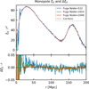 |
Fig. 3 Monopole of the 2PCF from FuGa3D and from exact pair counting (Corrfunc). The input catalogue is the full MICE simulation in z = 1.0–1.2. The FuGa3D results are shown for three resolution settings (see main text for details). The lower panel shows the difference with respect to the Corrfunc result. |
5.3 Power spectrum from discrete coordinates
In another test, we validated the accuracy of the point-source power spectrum computation described in Sect. 4. For this purpose, we computed the angular power spectrum for a single redshift shell z ∈ [1.0, 1.1]. We did this first using discrete coordinates, which is the default method in FuGa3D, and then with a map-based SHT. For the latter, we used an older version of FuGa3D, where this was implemented and maintained as an option for validation purposes. The test was run on a MacBook laptop with 8 cores.
Figure 5 shows the point-source based clustering spectrum, together with map-based spectra with resolution Nside=2048, 4096, 8192. The spectra shown are pseudo-spectra, i.e. not corrected for the survey footprint. As the resolution increases, the map-based spectrum approaches that from point source coordinates, validating the point-source algorithm. Computing the point-source spectrum took 22.1 s, while the map-based transform took 10.5 s, 20.3 s, 43.4 s, and 128.1 s with Nside=1024, 2048, 4096, 8192, respectively. Thus, the point-source transform is comparable in speed to the map-based transform with Nside=2048, it but reaches a much higher accuracy.
Figure 6 shows a similar comparison for the EE shear spectrum. Here, the uncorrected pseudo-spectra cannot be compared directly, since there is no common normalisation. Increasing the resolution further beyond the point where there is only one galaxy per pixel, scales the spectrum down as inversely proportional to the pixel size squared, ![Mathematical equation: $\[\propto 1 / N_{\text {side}}^{4}\]$](/articles/aa/full_html/2026/05/aa56027-25/aa56027-25-eq78.png) . To bring the spectra to a common normalisation, we scale each spectrum with the sky coverage, which we read from the ℓ = 0 element of the mask spectrum Wss.
. To bring the spectra to a common normalisation, we scale each spectrum with the sky coverage, which we read from the ℓ = 0 element of the mask spectrum Wss.
 |
Fig. 5 Angular clustering pseudo-spectrum from exact point-source coordinates and from maps of different resolutions. The lower panel shows the difference with respect to the point-source result. |
 |
Fig. 6 Same as Fig. 5 but for EE shear spectrum. The pseudo-spectra have been scaled by the sky fraction to make them comparable (see main text for explanation). |
5.4 Correlation function from power spectrum
In the third validation test, we compared correlation functions computed directly or from power spectra. We selected the redshift range z ∈ [1.0, 1.1] for consideration and computed the angular correlation function in two ways. First, we computed the correlation function through the modified LS, as described in Sects. 3.3 and 3.4. We refer to this as the ‘direct method’. As an alternative method, we (1) computed the angular power spectrum using the exact galaxy coordinates, (2) subtracted an estimate for the shot noise, which we obtained as the mean of the last 500 multipoles, (3) applied the kernel correction as described in Sect. 4.2, and (4) transformed the power spectrum into a correlation function as per Sect. 2.3. The results are shown in Figs. 7 and 8. The clustering correlation function from these two different methods agrees very well, further validating our code.
5.5 Considerations of speed
Figure 9 shows the CPU cost of computing the RCF for the redshift range z = 1.0–1.2 with FuGa3D, for different combinations of Nside and zΔ. All timing tests were run on a single node of the Puhti supercluster. We show separately the CPU cost with or without shear analysis. The dashed lines indicate the cases where the angular and redshift resolutions correspond to the same physical distance: (Nside = 512, zΔ = 0.0025), (Nside = 1024, zΔ = 0.001), and (Nside = 2048, zΔ = 0.0005). In the chosen redshift range, these combinations correspond roughly to a spatial resolution of 6 Mpc, 3 Mpc, and 1.5 Mpc, respectively. Changing both resolutions in unison is meaningful when the goal is to estimate the real-space correlation function. In tomographic analysis, one might be more interested in the CPU cost for a fixed redshift resolution. Results are shown for small and full MICE inputs, and with and without shear analysis.
We further study the CPU cost of the harmonic analysis. In Fig. 10 we show the CPU cost of computing the RP as a function of the ℓmax parameter. In this test, we fix the redshift resolution to zΔ=0.005 and compute the auto- and cross-spectra for |z1 − z2| < 0.1 in the range z ∈ 1.0–1.2. This involves computing the SHT for 40 redshift bins, and constructing spectra for 630 pairs of bins. We show the cost of computing the raw pseudo-spectrum for the small and the full MICE catalogues, with and without shear analysis. In the same graph, we also show the cost of the post-processing step that corrects for the survey mask. The cost of full power-spectrum analysis is the sum of the cost of pseudospectrum estimation and that of post-processing.
The post-processing cost is dominated by the construction of the coupling kernel and inverting it. The kernel correction does not depend on the catalogue size; thus the cost is the same for the small or the full catalogue. As explained in Sect. 4.2, a single coupling kernel applies to all clustering spectra, while for shear, each of the 630 redshift pairs has its own kernel, which depends on the distribution of the galaxies. For this reason, the kernel correction is orders of magnitude more expensive in the shear analysis.
 |
Fig. 7 Angular clustering correlation from the direct computation (Nside=2048) or from the power spectrum (ℓmax=8000). The bottom panel shows the difference. The redshift range is z ∈ [1.0, 1.1]. |
 |
Fig. 9 CPU cost of RCF computation. We show the CPU cost as a function of pixel resolution Nside, with different redshift resolutions zΔ for clustering (top) or for clustering and shear (bottom). The redshift resolution is, from top down, zΔ=0.0005 (blue), zΔ=0.001 (yellow), zΔ=0.0025 (green), and zΔ=0.005 (red). The dashed lines connect points where Nside and zΔ correspond to the same spatial resolution (from left to right, 6 Mpc, 3 Mpc, 1.5 Mpc). The input data is the full (circles) or the small (triangles) MICE simulation in z = 1.0–1.2. To guide the eye, one node-hour and one node-minute have been indicated by horizontal lines. |
 |
Fig. 10 CPU cost of harmonic-space analysis for 630 redshift-shell pairs. Shown is the cost of computing the redshift–space pseudospectrum for ℓmax=2000–8000 for full (circles) and small (triangles) MICE in z = 1.0–1.2. The redshift resolution was fixed at zΔ=0.005. The squares indicate the cost of constructing the mode-mode coupling kernel to correct for the survey footprint. |
6 Conclusions
We have studied the RCF and its harmonic counterpart, the RP, as tools in the analysis of large galaxy catalogues. Since these data objects do not depend on the distance-redshift relation, they provide a model-independent characterisation of the statistical properties of a galaxy distribution.
We have developed the FuGa3D code. This code constructs the RCF and its RP data objects, and it provides a number of post-processing tools. The direct RCF computation is based on a modified Landy–Szalay estimator and relies on a discretised spherical grid and on the assumption that the selection function is piecewise isotropic in the survey light-cone. The code is efficient, computing the RCF and the 2PCF for the full MICE simulation in z = 1.0–1.2 at resolution settings that correspond to 1.5 Mpc spatial resolution (nside=2048, zΔ=0.0005). This process took 47 node-min for clustering only and 7.3 node-hours with shear analysis included. Relaxing the resolution to 3 Mpc drops the times to 12 node-min for clustering and to 3 node-hours for clustering and shear.
We have demonstrated the usefulness of the RCF in the estimation of the real-space 2PCF. Once the RCF data object has been constructed and stored, computing the real-space 2PCF for any given cosmology is a very fast process. One can examine a space of cosmological parameters with a short turnaround time and without a full recomputation of the correlation function.
The FuGa3D code estimates power spectra using the exact coordinates of the galaxies and thus requires discretisation only in the radial dimension. The power spectrum can be converted to a correlation function with the help of Wigner functions, providing an alternative way of constructing the RCF. The question of which of the two methods is the most efficient cannot be answered definitively because different parts of the code scale differently, and the optimal parameter settings depend on the characteristics of the dataset and on the accuracy requirements. Both methods have their benefits and drawbacks. The direct method requires less run time memory than the power-spectrum procedure. The latter has a large memory footprint because a large number of SHTs must be kept in memory simultaneously to construct the cross-spectra between (zk, zk′) bins. The power-spectrum approach, on the other hand, offers the benefit of accommodating an arbitrary selection function, while the direct method relies on a piecewise isotropic selection function. This limitation arises from the speed-up algorithm implemented in FuGa3D rather than from any intrinsic property of the RCF. Given sufficient computational resources, a full Landy–Szalay estimator could be employed for constructing the RCF without restriction.
In this paper, we concentrated on the algorithmic aspects of the FuGa3D code package. Several important development ideas are left for future work. For instance, a potential future improvement involves handling redshift uncertainty. The current approach assumes perfect redshift measurements and assigns each galaxy to a single shell. To account for imprecise redshifts, galaxies could instead be represented by a probability distribution reflecting the uncertainty in their redshift estimates.
Another important future development is to test the use of RCF in the context of cosmological parameter estimation. The RCF approach offers the benefit that it does not involve a fiducial cosmological model. The RCF can be used in a parameter sampling loop in two different ways:
Pre-compute the RCF once for the dataset. At every sampling step, convert the RCF to a real-space correlation function using the current parameter values and evaluate the likelihood at the 2PCF level. This ensures that the 2PCF is always consistent with the sampling parameters. The data vector for a likelihood in this case is the 2PCF;
Use the pre-computed RCF itself as the dataset. At each sampling step, construct a model for the RCF using the current parameters and evaluate the likelihood at the RCF level. The data vector in this case is the RCF.
The first approach is more straightforward, as it can largely be realised using existing software tools with relatively little extra work. The second approach involves the more demanding step of modelling the RCF from a given cosmology or from a matter power spectrum provided by a standard software tool, such as CAMB. Nonetheless, the second approach is conceptually simpler in the sense that it does not involve modifying the data between sampling steps.
Parameter sampling requires an estimate for the covariance of the data. The FuGa3D code provides a diagonal covariance estimate that is based on number counts, and thus it captures the Poisson part of the full covariance. Because FuGa3D is very fast, a full covariance could be constructed as a sample covariance from a number of mock catalogues, possibly accompanied by a smoothing or regularisation step, but this remains to be tested. An interesting question is whether the RCF can be compressed in some way without losing information. All of this is a field of study on its own right and is left for future work.
Data availability
The FuGa3D code is available via https://wiki.helsinki.fi/xwiki/bin/view/FuGa3D/.
Acknowledgements
This work has been supported by the Research Council of Finland grant 34 7088, and the Jenny and Antti Wihuri Foundation. The authors wish to acknowledge CSC – IT Center for Science, Finland, for computational resources.
References
- Abazajian, K. N., Adelman-McCarthy, J. K., Agüeros, M. A., et al. 2009, ApJS, 182, 543 [Google Scholar]
- Akeson, R., Armus, L., Bachelet, E., et al. 2019, arXiv e-prints [arXiv:1902.05569] [Google Scholar]
- Alcock, C., & Paczynski, B. 1979, Nature, 281, 358 [NASA ADS] [CrossRef] [Google Scholar]
- Baleato Lizancos, A., & White, M. 2024, JCAP, 05, 010 [Google Scholar]
- Ballinger, W. E., Peacock, J. A., & Heavens, A. F. 1996, MNRAS, 282, 877 [NASA ADS] [CrossRef] [Google Scholar]
- Bautista, J. E., Paviot, R., Vargas Magaña, M., et al. 2021, MNRAS, 500, 736 [Google Scholar]
- Beutler, F., Blake, C., Colless, M., et al. 2012, MNRAS, 423, 3430 [NASA ADS] [CrossRef] [Google Scholar]
- Brown, M. L., Castro, P. G., & Taylor, A. N. 2005, MNRAS, 360, 1262 [NASA ADS] [CrossRef] [Google Scholar]
- Camphuis, E., Benabed, K., Galli, S., Hivon, E., & Lilley, M. 2022, A&A, 668, A62 [NASA ADS] [CrossRef] [EDP Sciences] [Google Scholar]
- Challinor, A., & Chon, G. 2005, MNRAS, 360, 509 [NASA ADS] [CrossRef] [Google Scholar]
- Colless, M., Peterson, B. A., Jackson, C., et al. 2003, arXiv e-prints [arXiv:astro-ph/0306581] [Google Scholar]
- Crocce, M., Castander, F. J., Gaztañaga, E., Fosalba, P., & Carretero, J. 2015, MNRAS, 453, 1513 [NASA ADS] [CrossRef] [Google Scholar]
- Dark Energy Survey Collaboration (Abbott, T., et al.) 2016, MNRAS, 460, 1270 [Google Scholar]
- DESI Collaboration (Abdul-Karim, M., et al.) 2025, arXiv e-prints [arXiv:2503.14745] [Google Scholar]
- Euclid Collaboration (Mellier, Y., et al.) 2025, A&A, 697, A1 [Google Scholar]
- Euclid Collaboration (Tessore, N., et al.) 2025, A&A, 694, A141 [Google Scholar]
- Fosalba, P., Crocce, M., Gaztañaga, E., & Castander, F. J. 2015a, MNRAS, 448, 2987 [NASA ADS] [CrossRef] [Google Scholar]
- Fosalba, P., Gaztañaga, E., Castander, F. J., & Crocce, M. 2015b, MNRAS, 447, 1319 [NASA ADS] [CrossRef] [Google Scholar]
- Górski, K. M., Hivon, E., Banday, A. J., et al. 2005, ApJ, 622, 759 [Google Scholar]
- Guzzo, L., Pierleoni, M., Meneux, B., et al. 2008, Nature, 451, 541 [Google Scholar]
- Heymans, C., Tröster, T., Asgari, M., et al. 2021, A&A, 646, A140 [NASA ADS] [CrossRef] [EDP Sciences] [Google Scholar]
- Hivon, E., Górski, K. M., Netterfield, C. B., et al. 2002, ApJ, 567, 2 [NASA ADS] [CrossRef] [Google Scholar]
- Hou, J., Sánchez, A. G., Scoccimarro, R., et al. 2018, MNRAS, 480, 2521 [NASA ADS] [CrossRef] [Google Scholar]
- Ivezić, Ž., Kahn, S. M., Tyson, J. A., et al. 2019, ApJ, 873, 111 [Google Scholar]
- Kaiser, N. 1987, MNRAS, 227, 1 [Google Scholar]
- Keihänen, E., Kurki-Suonio, H., Lindholm, V., et al. 2019, A&A, 631, A73 [NASA ADS] [CrossRef] [EDP Sciences] [Google Scholar]
- Kilbinger, M. 2015, Rep. Progr. Phys., 78, 086901 [Google Scholar]
- Landy, S. D., & Szalay, A. S. 1993, ApJ, 412, 64 [Google Scholar]
- Li, X., Zhang, T., Sugiyama, S., et al. 2023, Phys. Rev. D, 108, 123518 [CrossRef] [Google Scholar]
- Okumura, T., Matsubara, T., Eisenstein, D. J., et al. 2008, ApJ, 676, 889 [Google Scholar]
- Peacock, J. A., Cole, S., Norberg, P., et al. 2001, Nature, 410, 169 [Google Scholar]
- Peebles, P. J. E. 1980, The Large-scale Structure of the Universe (Princeton University Press) [Google Scholar]
- Reid, B. A., Samushia, L., White, M., et al. 2012, MNRAS, 426, 2719 [NASA ADS] [CrossRef] [Google Scholar]
- Reinecke, M., Belkner, S., & Carron, J. 2023, A&A, 678, A165 [NASA ADS] [CrossRef] [EDP Sciences] [Google Scholar]
- Salazar-Albornoz, S., Sánchez, A. G., Padilla, N. D., & Baugh, C. M. 2014, MNRAS, 443, 3612 [NASA ADS] [CrossRef] [Google Scholar]
- Schneider, P., van Waerbeke, L., Kilbinger, M., & Mellier, Y. 2002, A&A, 396, 1 [NASA ADS] [CrossRef] [EDP Sciences] [Google Scholar]
- Schulten, K., & Gordon, R. G. 1975, J. Math. Phys., 16, 1961 [Google Scholar]
- Sinha, M., & Garrison, L. H. 2020, MNRAS, 491, 3022 [Google Scholar]
- Varshalovich, D. A., Moskalev, A. N., & Khersonskii, V. K. 1988, Quantum Theory of Angular Momentum (World Scientific Publishing Company) [Google Scholar]
- York, D. G., Adelman, J., Anderson, Jr., J. E., et al. 2000, AJ, 120, 1579 [NASA ADS] [CrossRef] [Google Scholar]
- Zarrouk, P., Burtin, E., Gil-Marín, H., et al. 2018, MNRAS, 477, 1639 [NASA ADS] [CrossRef] [Google Scholar]
Appendix A From power spectrum to correlation function
Here we derive the relation between the angular correlation function and the power spectrum. We expand the density contrast and the shear field in spin-spherical harmonics,
![Mathematical equation: $\[\begin{aligned}\delta(\vartheta, \varphi) & =\sum_{\ell m} a_{\ell m ~0} Y_{\ell m}(\vartheta, \varphi) \\\left(\gamma_1 \pm \mathrm{i} \gamma_2\right)(\vartheta, \varphi) & =\sum_{\ell m} \pm 2 a_{\ell m ~\pm 2} Y_{\ell m}(\vartheta, \varphi)=-\left(a_{E \ell m} \pm \mathrm{i} a_{B \ell m}\right)_{ \pm 2} Y_{\ell m}(\vartheta, \varphi).\end{aligned}\]$](/articles/aa/full_html/2026/05/aa56027-25/aa56027-25-eq79.png) (A.1)
(A.1)
The γ1 and γ2 components can be solved from this as
![Mathematical equation: $\[\begin{aligned}& \gamma_1(\vartheta, \varphi)=-\frac{1}{2} \sum_{\ell m} a_{E \ell m}({ }_2 Y_{\ell m}(\vartheta, \varphi)+{ }_{-2} Y_{\ell m}(\vartheta, \varphi))-\frac{\mathrm{i}}{2} \sum_{\ell m} a_{B \ell m}({ }_2 Y_{\ell m}(\vartheta, \varphi)-{ }_{-2} Y_{\ell m}(\vartheta, \varphi)), \\& \gamma_2(\vartheta, \varphi)=-\frac{1}{2} \sum_{\ell m} a_{B \ell m}({ }_2 Y_{\ell m}(\vartheta, \varphi)+{ }_{-2} Y_{\ell m}(\vartheta, \varphi))+\frac{\mathrm{i}}{2} \sum_{\ell m} a_{E \ell m}({ }_2 Y_{\ell m}(\vartheta, \varphi)-{ }_{-2} Y_{\ell m}(\vartheta, \varphi)).\end{aligned}\]$](/articles/aa/full_html/2026/05/aa56027-25/aa56027-25-eq80.png) (A.2)
(A.2)
The clustering correlation function is
![Mathematical equation: $\[\xi(\theta)=\langle\delta^*(\vartheta, \varphi) \delta(\vartheta^{\prime}, \varphi^{\prime})\rangle=\sum_{\ell m} \sum_{\ell^{\prime} m^{\prime}}\langle a_{\ell m}^* a_{\ell^{\prime} m^{\prime}}\rangle_0 Y_{\ell m}^*(\vartheta, \varphi)_0 Y_{\ell^{\prime} m^{\prime}}(\vartheta^{\prime}, \varphi^{\prime})=\sum_{\ell} P_{\ell} \sum_m{ }_0 Y_{\ell m}^*(\vartheta, \varphi)_0 Y_{\ell m}(\vartheta^{\prime}, \varphi^{\prime}),\]$](/articles/aa/full_html/2026/05/aa56027-25/aa56027-25-eq81.png) (A.3)
(A.3)
where θ is the angular separation between points (ϑ, φ) and (ϑ′, φ′). Other correlation components involve similar combinations of two spin harmonics. We introduce the short-hand notation Sℓ,s1,s2 and write, using the general addition theorem of spin harmonics,
![Mathematical equation: $\[S_{\ell, s_1, s_2} \equiv \sum_m s_1 Y_{\ell m}^*(\vartheta, \varphi)_{s_2} Y_{\ell m}(\vartheta^{\prime}, \varphi^{\prime})=\sqrt{\frac{2 \ell+1}{4 \pi}} s_2 Y_{\ell,-s_1}(\theta, \phi) \mathrm{e}^{-\mathrm{i} s_2 \psi}=\sqrt{\frac{2 \ell+1}{4 \pi}} d_{-s_1,-s_2}^{\ell}(\theta) \mathrm{e}^{-\mathrm{i} s_1 \phi} \mathrm{e}^{-\mathrm{i} s_2 \psi},\]$](/articles/aa/full_html/2026/05/aa56027-25/aa56027-25-eq82.png) (A.4)
(A.4)
where ϕ, θ, ψ are the Euler angles that rotate (ϑ, φ) to (ϑ′, φ′). In the last equality, we expressed the spherical harmonic in terms of the reduced Wigner function. From the symmetry properties of Wigner functions, it follows that Sℓ,2,2 = Sℓ,−2,−2, Sℓ,2,−2 = Sℓ,−2,2, and Sℓ,0,2 = Sℓ,2,0 = Sℓ,−2,0 = Sℓ,0,−2.
Without loss of generality, we can place the pair of points on the same meridian, so that ϕ = ψ = 0, and θ remains as the angular separation between the points. We can then interpret γt = γ1 and γ× = γ2, where γt and γ× are the tangential and cross shear components, respectively (see Eq. 6). The independent components are then
![Mathematical equation: $\[S_{\ell, 0,0}=\sqrt{\frac{2 \ell+1}{4 \pi}} d_{0,0}^{\ell}(\theta), \quad S_{\ell, 2,2}=\sqrt{\frac{2 \ell+1}{4 \pi}} d_{2,0}^{\ell}(\theta), \quad S_{\ell, 2,-2}=\sqrt{\frac{2 \ell+1}{4 \pi}} d_{2,-2}^{\ell}(\theta).\]$](/articles/aa/full_html/2026/05/aa56027-25/aa56027-25-eq83.png) (A.5)
(A.5)
We can now construct the correlators:
![Mathematical equation: $\[\begin{aligned}\xi_{\mathrm{cc}}(\theta)=\langle\delta^* \delta\rangle= & P_{\ell}^{C C} S_{\ell, 0,0}, \\\xi_{\mathrm{ct}}(\theta)=\langle\delta^* \gamma_1\rangle= & -\frac{1}{2} P_{\ell}^{C E}(S_{\ell, 0,2}+S_{\ell, 0,-2})-\frac{1}{2} P_{\ell}^{C B}(S_{\ell, 0,2}-S_{\ell, 0,-2})=-P_{\ell}^{C E} S_{\ell, 0,2}, \\\xi_{\mathrm{c} \times}(\theta)=\langle\delta^* \gamma_2\rangle= & -\frac{1}{2} P_{\ell}^{C B}(S_{\ell, 0,2}+S_{\ell, 0,-2})+\frac{1}{2} P_{\ell}^{C E}(S_{\ell, 0,2}-S_{\ell, 0,-2})=-P_{\ell}^{C B} S_{\ell, 0,2}, \\\xi_{\mathrm{tt}}(\theta)=\langle\gamma_1^* \gamma_1\rangle= & \frac{1}{4} P_{\ell}^{E E}(S_{\ell, 2,2}+S_{\ell, 2,-2}+S_{\ell,-2,2}+S_{\ell,-2,-2})+\frac{1}{4} P_{\ell}^{B B}(S_{\ell, 2,2}-S_{\ell, 2,-2}-S_{\ell,-2,2}+S_{\ell,-2,-2}) \\& \quad+\frac{\mathrm{i}}{4} P_{\ell}^{E B}(S_{\ell, 2,2}-S_{\ell, 2,-2}+S_{\ell,-2,2}-S_{\ell,-2,-2}))+\frac{\mathrm{i}}{4} P_{\ell}^{B E}(-S_{\ell, 2,2}-S_{\ell, 2,-2}+S_{\ell,-2,2}+S_{\ell,-2,-2})) \\= & P_{\ell}^{E E}(S_{\ell, 2,2}+S_{\ell, 2,-2})+P_{\ell}^{B B}(S_{\ell, 2,2}-S_{\ell, 2,-2}), \\\xi_{\times \times}(\theta)=\langle\gamma_2 \gamma_2\rangle= & \frac{1}{4} P_{\ell}^{B B}(S_{\ell, 2,2}+S_{\ell, 2,-2}+S_{\ell,-2,2}+S_{\ell,-2,-2})+\frac{1}{4} P_{\ell}^{E E}(S_{\ell, 2,2}-S_{\ell, 2,-2}-S_{\ell,-2,2}+S_{\ell,-2,-2}) \\= & P_{\ell}^{B B}(S_{\ell, 2,2}+S_{\ell, 2,-2})+P_{\ell}^{E E}(S_{\ell, 2,2}-S_{\ell, 2,-2}), \\\xi_{\mathrm{t} \times}(\theta)=\langle\gamma_1 \gamma_2\rangle= & \frac{1}{4} P_{\ell}^{E B}(S_{\ell, 2,2}+S_{\ell, 2,-2}+S_{\ell,-2,2}+S_{\ell,-2,-2})+\frac{1}{4} P_{\ell}^{B E}(-S_{\ell, 2,2}+S_{\ell, 2,-2}+S_{\ell,-2,2}-S_{\ell,-2,-2}) \\= & P_{\ell}^{E B}(S_{\ell, 2,2}+S_{\ell, 2,-2})+P_{\ell}^{B E}(-S_{\ell, 2,2}+S_{\ell, 2,-2}), \\\xi_{\times \mathrm{t}}(\theta)=\langle\gamma_2 \gamma_1\rangle= & \frac{1}{4} P_{\ell}^{B E}(S_{\ell, 2,2}+S_{\ell, 2,-2}+S_{\ell,-2,2}+S_{\ell,-2,-2})+\frac{1}{4} P_{\ell}^{E B}(-S_{\ell, 2,2}+S_{\ell, 2,-2}+S_{\ell,-2,2}-S_{\ell,-2,-2})) \\= & P_{\ell}^{B E}(S_{\ell, 2,2}+S_{\ell, 2,-2})+P_{\ell}^{E B}(-S_{\ell, 2,2}+S_{\ell, 2,-2}).\end{aligned}\]$](/articles/aa/full_html/2026/05/aa56027-25/aa56027-25-eq84.png) (A.6)
(A.6)
After the line for ξtt we did not explicitly write the imaginary elements, which vanish anyway. The correlated fields here may represent two different fields, for instance from two redshift shells. For this reason the ordering of the elements on the right-hand side is relevant, and in general ![Mathematical equation: $\[P_{\ell}^{E B} \neq P_{\ell}^{B E}\]$](/articles/aa/full_html/2026/05/aa56027-25/aa56027-25-eq85.png) .
.
The correlations can be combined into independent combinations as
![Mathematical equation: $\[\begin{aligned}\xi_{\mathrm{cc}}(\theta) & =\sum_{\ell} \frac{2 \ell+1}{4 \pi} C_{\ell}^{C C} d_{00}^{\ell}(\theta), \\\xi_{+}(\theta) & =\sum_{\ell} \frac{2 \ell+1}{4 \pi}\left(C_{\ell}^{E E}+C_{\ell}^{B B}\right) d_{2,2}^{\ell}(\theta), \\\xi_{-}(\theta) & =\sum_{\ell} \frac{2 \ell+1}{4 \pi}\left(C_{\ell}^{E E}-C_{\ell}^{B B}\right) d_{2,-2}^{\ell}(\theta), \\\xi_{\mathrm{ct}}(\theta) & =-\sum_{\ell} \frac{2 \ell+1}{4 \pi} C_{\ell}^{C E} d_{20}^{\ell}(\theta), \\\xi_{\mathrm{c} \times}(\theta) & =-\sum_{\ell} \frac{2 \ell+1}{4 \pi} C_{\ell}^{C B} d_{20}^{\ell}(\theta), \\\xi_{\mathrm{t} \times}(\theta)+\xi_{\times \mathrm{t}}(\theta) & =\sum_{\ell} \frac{2 \ell+1}{4 \pi}\left(C_{\ell}^{E B}+C_{\ell}^{B E}\right) d_{2,-2}^{\ell}(\theta), \\\xi_{\mathrm{t} \times}(\theta)-\xi_{\times \mathrm{t}}(\theta) & =\sum_{\ell} \frac{2 \ell+1}{4 \pi}\left(C_{\ell}^{E B}-C_{\ell}^{B E}\right) d_{2,2}^{\ell}(\theta).\end{aligned}\]$](/articles/aa/full_html/2026/05/aa56027-25/aa56027-25-eq86.png) (A.7)
(A.7)
Note that ![Mathematical equation: $\[d_{00}^{\ell}(\theta)=L_{\ell}(\cos~ \theta)\]$](/articles/aa/full_html/2026/05/aa56027-25/aa56027-25-eq87.png) , where Lℓ is the Legendre polynomial. These relations can be inverted using the orthogonality of the reduced Wigner functions
, where Lℓ is the Legendre polynomial. These relations can be inverted using the orthogonality of the reduced Wigner functions
![Mathematical equation: $\[\int_0^\pi d_{s s^{\prime}}^{\ell}(\theta) d_{s s^{\prime}}^{\ell^{\prime}}(\theta) ~\sin~ \theta ~\mathrm{d} \theta=\frac{2}{2 \ell+1} \delta_{\ell \ell^{\prime}}.\]$](/articles/aa/full_html/2026/05/aa56027-25/aa56027-25-eq88.png) (A.8)
(A.8)
Appendix B Coupling kernel
The density field observed under a binary sky mask wc(ϑ, φ)= 1, 0 is
![Mathematical equation: $\[\hat{\delta}(\vartheta, \varphi)=\delta(\vartheta, \varphi) w^{\mathrm{c}}(\vartheta, \varphi)=\sum_{\ell^{\prime} m^{\prime}} \sum_{\ell^{\prime \prime} m^{\prime \prime}} a_{\ell^{\prime} m^{\prime}} \omega_{\ell^{\prime \prime} m^{\prime \prime}} Y_{\ell^{\prime} m^{\prime}}(\vartheta, \varphi) Y_{\ell^{\prime \prime} m^{\prime \prime}}(\vartheta, \varphi).\]$](/articles/aa/full_html/2026/05/aa56027-25/aa56027-25-eq89.png) (B.1)
(B.1)
Similarly, for shear,
![Mathematical equation: $\[\left(\hat{\gamma}_1 \pm \mathrm{i} \hat{\gamma}_2\right)(\vartheta, \varphi)=\left(\gamma_1+\mathrm{i} \gamma_2\right)(\vartheta, \varphi) \omega^{\mathrm{s}}(\vartheta, \varphi)=\sum_{\ell^{\prime} m^{\prime}} \sum_{\ell^{\prime \prime} m^{\prime \prime}}{ }_{ \pm 2} a_{\ell^{\prime} m^{\prime}} \omega_{\ell^{\prime \prime} m^{\prime \prime} \pm 2}^{\mathrm{s}} Y_{\ell^{\prime} m^{\prime}}(\vartheta, \varphi) Y_{\ell^{\prime \prime} m^{\prime \prime}}(\vartheta, \varphi).\]$](/articles/aa/full_html/2026/05/aa56027-25/aa56027-25-eq90.png) (B.2)
(B.2)
The SHT of the masked field yields
![Mathematical equation: $\[\hat{a}_{\ell m}=\int \hat{\delta}(\vartheta, \varphi) Y_{\ell m}^*(\vartheta, \varphi) \mathrm{d} \Omega=\sum_{\ell^{\prime} m^{\prime}} \sum_{\ell^{\prime \prime} m^{\prime \prime}} a_{\ell^{\prime} m^{\prime}} \omega_{\ell^{\prime \prime} m^{\prime \prime}}^{\mathrm{c}} \int Y_{\ell m}^*(\vartheta, \varphi) Y_{\ell^{\prime} m^{\prime}}(\vartheta, \varphi) Y_{\ell^{\prime \prime} m^{\prime \prime}}(\vartheta, \varphi) \mathrm{d} \Omega\]$](/articles/aa/full_html/2026/05/aa56027-25/aa56027-25-eq91.png) (B.3)
(B.3)
and
![Mathematical equation: $\[{ }_{ \pm 2} \hat{a}_{\ell m}=\int\left(\hat{\gamma}_1 \pm \hat{\gamma}_2\right)(\vartheta, \varphi)_{ \pm 2} Y_{\ell m}^*(\vartheta, \varphi) \mathrm{d} \Omega=\sum_{\ell^{\prime} m^{\prime}} \sum_{\ell^{\prime \prime} m^{\prime \prime}}{ }_{ \pm 2} a_{\ell^{\prime} m^{\prime}} \omega_{\ell^{\prime \prime} m^{\prime \prime}}^{\mathrm{s}} \int{ }_{ \pm 2} Y_{\ell m}^*(\vartheta, \varphi)_{ \pm 2} Y_{\ell^{\prime} m^{\prime}}(\vartheta, \varphi) Y_{\ell^{\prime \prime} m^{\prime \prime}}(\vartheta, \varphi) ~\mathrm{d} \Omega.\]$](/articles/aa/full_html/2026/05/aa56027-25/aa56027-25-eq92.png) (B.4)
(B.4)
Using the symmetry property ![Mathematical equation: $\[{ }_{s} Y_{\ell m}^{*}(\vartheta, \varphi)=(-1)^{m+s}{ }_{-s} Y_{\ell-m}(\vartheta, \varphi)\]$](/articles/aa/full_html/2026/05/aa56027-25/aa56027-25-eq93.png) and the expression of the triple integral in terms of Wigner 3j symbols,
and the expression of the triple integral in terms of Wigner 3j symbols,
![Mathematical equation: $\[\int{ }_s Y_{\ell m}^*(\vartheta, \varphi)_{s^{\prime}} Y_{\ell^{\prime} m^{\prime}}(\vartheta, \varphi)_{s^{\prime \prime}} Y_{\ell^{\prime \prime} m^{\prime \prime}}(\vartheta, \varphi) ~\mathrm{d} \Omega=F\left(\ell, \ell^{\prime}, \ell^{\prime \prime}\right)\left(\begin{array}{ccc}\ell & \ell^{\prime} & \ell^{\prime \prime} \\m & m^{\prime} & m^{\prime \prime}\end{array}\right)\left(\begin{array}{ccc}\ell & \ell^{\prime} & \ell^{\prime \prime} \\-s & -s^{\prime} & -s^{\prime \prime}\end{array}\right),\]$](/articles/aa/full_html/2026/05/aa56027-25/aa56027-25-eq94.png) (B.5)
(B.5)
where
![Mathematical equation: $\[F\left(\ell, \ell^{\prime}, \ell^{\prime \prime}\right)=\left[\frac{(2 \ell+1)\left(2 \ell^{\prime}+1\right)\left(2 \ell^{\prime \prime}+1\right)}{4 \pi}\right]^{1 / 2},\]$](/articles/aa/full_html/2026/05/aa56027-25/aa56027-25-eq95.png) (B.6)
(B.6)
we arrive at
![Mathematical equation: $\[\hat{a}_{\ell m}=\sum_{\ell^{\prime} m^{\prime}} \sum_{\ell^{\prime \prime} m^{\prime \prime}} \omega_{\ell^{\prime \prime} m^{\prime \prime}}^{\mathrm{c}}(-1)^m F\left(\ell, \ell^{\prime}, \ell^{\prime \prime}\right)\left(\begin{array}{ccc}\ell & \ell^{\prime} & \ell^{\prime \prime} \\0 & 0 & 0\end{array}\right)\left(\begin{array}{ccc}\ell & \ell^{\prime} & \ell^{\prime \prime} \\-m & m^{\prime} & m^{\prime \prime}\end{array}\right) a_{\ell^{\prime} m^{\prime}}\]$](/articles/aa/full_html/2026/05/aa56027-25/aa56027-25-eq96.png) (B.7)
(B.7)
and
![Mathematical equation: $\[{ }_{ \pm 2} \hat{a}_{\ell m}=\sum_{\ell^{\prime} m^{\prime}} \sum_{\ell^{\prime \prime} m^{\prime \prime}} \omega_{\ell^{\prime \prime} m^{\prime \prime}}^{\mathrm{s}}(-1)^m F\left(\ell, \ell^{\prime}, \ell^{\prime \prime}\right)\left(\begin{array}{ccc}\ell & \ell^{\prime} & \ell^{\prime \prime} \\\pm 2 & \mp 2 & 0\end{array}\right)\left(\begin{array}{ccc}\ell & \ell^{\prime} & \ell^{\prime \prime} \\-m & m^{\prime} & m^{\prime \prime}\end{array}\right){ }_{ \pm 2} a_{\ell^{\prime} m^{\prime}}.\]$](/articles/aa/full_html/2026/05/aa56027-25/aa56027-25-eq97.png) (B.8)
(B.8)
Further with ![Mathematical equation: $\[\hat{a}_{E \ell m}=-\frac{1}{2}\left({ }_{2} \hat{a}_{\ell m}+{ }_{-2} \hat{a}_{\ell m}\right), \hat{a}_{B \ell m}=\frac{\mathrm{i}}{2}\left({ }_{2} \hat{a}_{\ell m}-{ }_{-2} \hat{a}_{\ell m}\right)\]$](/articles/aa/full_html/2026/05/aa56027-25/aa56027-25-eq98.png) and ±2aℓm = −(aEℓm ± iaBℓm), and the symmetry relation
and ±2aℓm = −(aEℓm ± iaBℓm), and the symmetry relation
![Mathematical equation: $\[\left(\begin{array}{ccc}\ell & \ell^{\prime} & \ell^{\prime \prime} \\-2 & 2 & 0\end{array}\right)=(-1)^{\ell+\ell^{\prime}+\ell^{\prime \prime}}\left(\begin{array}{ccc}\ell & \ell^{\prime} & \ell^{\prime \prime} \\2 & -2 & 0\end{array}\right),\]$](/articles/aa/full_html/2026/05/aa56027-25/aa56027-25-eq99.png) (B.9)
(B.9)
we find
![Mathematical equation: $\[\begin{aligned}& \hat{a}_{E \ell m}=\sum_{\ell^{\prime} m^{\prime}} \sum_{\ell^{\prime \prime} m^{\prime \prime}} \omega_{\ell^{\prime \prime} m^{\prime \prime}}^{\mathrm{s}}(-1)^m F\left(\ell, \ell^{\prime}, \ell^{\prime \prime}\right)\left(\begin{array}{ccc}\ell & \ell^{\prime} & \ell^{\prime \prime} \\2 & -2 & 0\end{array}\right)\left(\begin{array}{ccc}\ell & \ell^{\prime} & \ell^{\prime \prime} \\-m & m^{\prime} & m^{\prime \prime}\end{array}\right)\left[\frac{1}{2} a_{E \ell^{\prime} m^{\prime}}\left(1+(-1)^{\ell+\ell^{\prime}+\ell^{\prime \prime}}\right)+\frac{\mathrm{i}}{2} a_{B \ell^{\prime} m^{\prime}}\left(1-(-1)^{\ell+\ell^{\prime}+\ell^{\prime \prime}}\right)\right], \\& \hat{a}_{B \ell m}=\sum_{\ell^{\prime} m^{\prime}} \sum_{\ell^{\prime \prime} m^{\prime \prime}} \omega_{\ell^{\prime \prime} m^{\prime \prime}}^{\mathrm{s}}(-1)^m F\left(\ell, \ell^{\prime}, \ell^{\prime \prime}\right)\left(\begin{array}{ccc}\ell & \ell^{\prime} & \ell^{\prime \prime} \\2 & -2 & 0\end{array}\right)\left(\begin{array}{ccc}\ell & \ell^{\prime} & \ell^{\prime \prime} \\-m & m^{\prime} & m^{\prime \prime}\end{array}\right)\left[\frac{1}{2} a_{B \ell^{\prime} m^{\prime}}\left(1+(-1)^{\ell+\ell^{\prime}+\ell^{\prime \prime}}\right)-\frac{\mathrm{i}}{2} a_{E \ell^{\prime} m^{\prime}}\left(1-(-1)^{\ell+\ell^{\prime}+\ell^{\prime \prime}}\right)\right].\end{aligned}\]$](/articles/aa/full_html/2026/05/aa56027-25/aa56027-25-eq100.png) (B.10)
(B.10)
The pseudo-spectrum for clustering is
![Mathematical equation: $\[\hat{P}_{\ell}=\frac{1}{2 \ell+1} \sum_m \hat{a}_{\ell m}^* \hat{a}_{\ell m}.\]$](/articles/aa/full_html/2026/05/aa56027-25/aa56027-25-eq101.png) (B.11)
(B.11)
Inserting the expression for ![Mathematical equation: $\[\hat{a}_{\ell m}\]$](/articles/aa/full_html/2026/05/aa56027-25/aa56027-25-eq102.png) and arranging the sums we find
and arranging the sums we find
![Mathematical equation: $\[\begin{aligned}\left\langle\hat{P}_{\ell}\right\rangle=\frac{1}{2 \ell+1} & \sum_{\ell^{\prime} \ell^{\prime \prime} \ell_1 \ell_2} F\left(\ell, \ell^{\prime}, \ell^{\prime \prime}\right) F\left(\ell, \ell_1, \ell_2\right)\left(\begin{array}{ccc}\ell & \ell^{\prime} & \ell^{\prime \prime} \\0 & 0 & 0\end{array}\right)\left(\begin{array}{ccc}\ell & \ell_1 & \ell_2 \\0 & 0 & 0\end{array}\right) \\& \quad \times \sum_{m m^{\prime} m^{\prime \prime} m_1 m_2} \omega_{\ell^{\prime \prime} m^{\prime \prime}}^{\mathrm{c}} \omega_{\ell_2 m_2}^{\mathrm{c}}\left(\begin{array}{ccc}\ell & \ell^{\prime} & \ell^{\prime \prime} \\-m & m^{\prime} & m^{\prime \prime}\end{array}\right)\left(\begin{array}{ccc}\ell & \ell_1 & \ell_2 \\-m & m_1 & m_2\end{array}\right)\left\langle a_{\ell^{\prime} m^{\prime}}^* a_{\ell_1 m_1}\right\rangle.\end{aligned}\]$](/articles/aa/full_html/2026/05/aa56027-25/aa56027-25-eq103.png) (B.12)
(B.12)
Using first
![Mathematical equation: $\[\left\langle a_{\ell^{\prime} m^{\prime}}^* a_{\ell_1 m_1}\right\rangle=\delta_{\ell^{\prime} \ell_1} \delta_{m^{\prime} m_1} P_{\ell}\]$](/articles/aa/full_html/2026/05/aa56027-25/aa56027-25-eq104.png) (B.13)
(B.13)
and then
![Mathematical equation: $\[\sum_{m m^{\prime}}\left(\begin{array}{ccc}\ell & \ell^{\prime} & \ell^{\prime \prime} \\-m & m^{\prime} & m^{\prime \prime}\end{array}\right)\left(\begin{array}{ccc}\ell & \ell_1 & \ell_2 \\-m & m_1 & m_2\end{array}\right)=\frac{1}{2 \ell^{\prime \prime}+1} \delta_{\ell^{\prime \prime} \ell_2} \delta_{m^{\prime \prime} m_2}\]$](/articles/aa/full_html/2026/05/aa56027-25/aa56027-25-eq105.png) (B.14)
(B.14)
and finally writing for the mask spectrum
![Mathematical equation: $\[\sum_{m^{\prime \prime}} \omega_{\ell^{\prime \prime} m^{\prime \prime}}^{\mathrm{c} *} \omega_{\ell^{\prime \prime} m^{\prime \prime}}^{\mathrm{c}}=\left(2 \ell^{\prime \prime}+1\right) W_{\ell^{\prime \prime}}^{\mathrm{cc}},\]$](/articles/aa/full_html/2026/05/aa56027-25/aa56027-25-eq106.png) (B.15)
(B.15)
we arrive at the final result:
![Mathematical equation: $\[\left\langle\hat{P}_{\ell}\right\rangle=\sum_{\ell^{\prime}} P_{\ell} \sum_{\ell^{\prime \prime}} W_{\ell^{\prime \prime}}^{\mathrm{cc}} \frac{1}{4 \pi}\left(2 \ell^{\prime}+1\right)\left(2 \ell^{\prime \prime}+1\right)\left(\begin{array}{ccc}\ell & \ell^{\prime} & \ell^{\prime \prime} \\0 & 0 & 0\end{array}\right)^2.\]$](/articles/aa/full_html/2026/05/aa56027-25/aa56027-25-eq107.png) (B.16)
(B.16)
From here one can read off the coupling kernel for clustering.
The other pseudo-spectra can be worked on in the same way. The reduction of the multiple sums happens in the same way, but we get a different combination of spectra on the right-hand side. Specifically, for the cross-spectra, the ℓ′ summation contains terms
![Mathematical equation: $\[\begin{aligned}& \left\langle\hat{P}_{\ell}^{C E}\right\rangle \propto\left\langle a_{\ell^{\prime} m^{\prime}}^*\left[\frac{1}{2} a_{E \ell^{\prime} m^{\prime}}\left(1+(-1)^{\ell+\ell^{\prime}+\ell^{\prime \prime}}\right)+\frac{\mathrm{i}}{2} a_{B \ell^{\prime} m^{\prime}}\left(1-(-1)^{\ell+\ell^{\prime}+\ell^{\prime \prime}}\right)\right]\right\rangle=\frac{1}{2}\left[P_{\ell^{\prime}}^{C E}\left(1+(-1)^{\ell+\ell^{\prime}+\ell^{\prime \prime}}\right)+\mathrm{i} P_{\ell^{\prime}}^{C B}\left(1-(-1)^{\ell+\ell^{\prime}+\ell^{\prime \prime}}\right)\right], \\& \left\langle\hat{P}_{\ell}^{C B}\right\rangle \propto\left\langle a_{\ell^{\prime} m^{\prime}}^*\left[\frac{1}{2} a_{B \ell^{\prime} m^{\prime}}\left(1+(-1)^{\ell+\ell^{\prime}+\ell^{\prime \prime}}\right)-\frac{\mathrm{i}}{2} a_{E \ell^{\prime} m^{\prime}}\left(1-(-1)^{\ell+\ell^{\prime}+\ell^{\prime \prime}}\right)\right]\right\rangle=\frac{1}{2}\left[P_{\ell^{\prime}}^{C B}\left(1+(-1)^{\ell+\ell^{\prime}+\ell^{\prime \prime}}\right)-\mathrm{i} P_{\ell^{\prime}}^{C E}\left(1-(-1)^{\ell+\ell^{\prime}+\ell^{\prime \prime}}\right)\right].\end{aligned}\]$](/articles/aa/full_html/2026/05/aa56027-25/aa56027-25-eq108.png) (B.17)
(B.17)
The full expressions for ![Mathematical equation: $\[\left\langle\hat{P}_{\ell}^{C E}\right\rangle\]$](/articles/aa/full_html/2026/05/aa56027-25/aa56027-25-eq109.png) and
and ![Mathematical equation: $\[\left\langle\hat{P}_{\ell}^{C B}\right\rangle\]$](/articles/aa/full_html/2026/05/aa56027-25/aa56027-25-eq110.png) include the Wigner symbol
include the Wigner symbol ![Mathematical equation: $\[\left(\begin{array}{ccc}\ell & \ell^{\prime} & \ell^{\prime \prime} \\ 0 & 0 & 0\end{array}\right)\]$](/articles/aa/full_html/2026/05/aa56027-25/aa56027-25-eq111.png) which vanishes for odd (ℓ + ℓ′ + ℓ″). We can assume (−1)ℓ+ℓ′+ℓ″ = 1, and we have simply
which vanishes for odd (ℓ + ℓ′ + ℓ″). We can assume (−1)ℓ+ℓ′+ℓ″ = 1, and we have simply ![Mathematical equation: $\[\left\langle\hat{P}_{\ell}^{C E}\right\rangle \propto P_{\ell^{\prime}}^{C E}\]$](/articles/aa/full_html/2026/05/aa56027-25/aa56027-25-eq112.png) and
and ![Mathematical equation: $\[\left\langle\hat{P}_{\ell}^{C B}\right\rangle \propto P_{\ell^{\prime}}^{C B}\]$](/articles/aa/full_html/2026/05/aa56027-25/aa56027-25-eq113.png) .
.
When working on the shear spectra, we must keep in mind that we are considering cross-spectra between two redshift shells. Thus the ordering of the elements is relevant, and ![Mathematical equation: $\[a_{E \ell m}^{*} a_{B \ell m} \neq a_{B \ell m} a_{E \ell m}^{*}\]$](/articles/aa/full_html/2026/05/aa56027-25/aa56027-25-eq114.png) .
.
![Mathematical equation: $\[\begin{aligned}& \left\langle\hat{P}_{\ell}^{E E}\right\rangle \propto\left\langle\left[\frac{1}{2} a_{E \ell^{\prime} m^{\prime}}^*\left(1+(-1)^{\ell+\ell^{\prime}+\ell^{\prime \prime}}\right)-\frac{\mathrm{i}}{2} a_{B \ell^{\prime} m^{\prime}}^*\left(1-(-1)^{\ell+\ell^{\prime}+\ell^{\prime \prime}}\right)\right]\left[\frac{1}{2} a_{E \ell^{\prime} m^{\prime}}\left(1+(-1)^{\ell+\ell^{\prime}+\ell^{\prime \prime}}\right)+\frac{\mathrm{i}}{2} a_{B \ell^{\prime} m^{\prime}}\left(1-(-1)^{\ell+\ell^{\prime}+\ell^{\prime \prime}}\right)\right]\right\rangle\\&\qquad\quad =\frac{1}{2} P_{\ell^{\prime}}^{E E}\left(1+(-1)^{\ell+\ell^{\prime}+\ell^{\prime \prime}}\right)+\frac{1}{2} P_{\ell^{\prime}}^{B B}\left(1-(-1)^{\ell+\ell^{\prime}+\ell^{\prime \prime}}\right),\end{aligned}\]$](/articles/aa/full_html/2026/05/aa56027-25/aa56027-25-eq115.png) (B.18)
(B.18)
where we used the fact that the factors ![Mathematical equation: $\[\frac{1}{2}\left(1 \pm(-1)^{\ell+\ell^{\prime}+\ell^{\prime \prime}}\right)\]$](/articles/aa/full_html/2026/05/aa56027-25/aa56027-25-eq116.png) are either 0 or 1, and thus
are either 0 or 1, and thus ![Mathematical equation: $\[\left[\frac{1}{2}\left(1 \pm(-1)^{\ell+\ell^{\prime}+\ell^{\prime \prime}}\right)\right]^{2}=\frac{1}{2}\left(1 \pm(-1)^{\ell+\ell^{\prime}+\ell^{\prime \prime}}\right)\]$](/articles/aa/full_html/2026/05/aa56027-25/aa56027-25-eq117.png) and (1 + (−1)ℓ+ℓ′+ℓ″)(1 − (−1)ℓ+ℓ′+ℓ″) = 0. A similar calculation for the other shear components gives
and (1 + (−1)ℓ+ℓ′+ℓ″)(1 − (−1)ℓ+ℓ′+ℓ″) = 0. A similar calculation for the other shear components gives
![Mathematical equation: $\[\begin{aligned}& \langle\hat{P}_{\ell}^{B B}\rangle \propto \frac{1}{2} P_{\ell^{\prime}}^{B B}(1+(-1)^{\ell+\ell^{\prime}+\ell^{\prime \prime}})+\frac{1}{2} P_{\ell^{\prime}}^{E E}(1-(-1)^{\ell+\ell^{\prime}+\ell^{\prime \prime}}), \\& \langle\hat{P}_{\ell}^{E B}\rangle \propto \frac{1}{2} P_{\ell^{\prime}}^{E B}(1+(-1)^{\ell+\ell^{\prime}+\ell^{\prime \prime}})-\frac{1}{2} P_{\ell^{\prime}}^{B E}(1-(-1)^{\ell+\ell^{\prime}+\ell^{\prime \prime}}), \\& \langle\hat{P}_{\ell}^{B E}\rangle \propto \frac{1}{2} P_{\ell^{\prime}}^{B E}(1+(-1)^{\ell+\ell^{\prime}+\ell^{\prime \prime}})-\frac{1}{2} P_{\ell^{\prime}}^{E B}(1-(-1)^{\ell+\ell^{\prime}+\ell^{\prime \prime}}).\end{aligned}\]$](/articles/aa/full_html/2026/05/aa56027-25/aa56027-25-eq118.png) (B.19)
(B.19)
The results can be arranged into natural components:
![Mathematical equation: $\[\begin{aligned}& \langle\hat{P}_{\ell}^{E E}+\hat{P}_{\ell}^{B B}\rangle \propto P_{\ell^{\prime}}^{E E}+P_{\ell^{\prime}}^{B B}, \\& \langle\hat{P}_{\ell}^{E E}-\hat{P}_{\ell}^{B B}\rangle \propto(P_{\ell^{\prime}}^{E E}-P_{\ell^{\prime}}^{B B})(-1)^{\ell+\ell^{\prime}+\ell^{\prime \prime}}, \\& \langle\hat{P}_{\ell}^{E B}+\hat{P}_{\ell}^{B E}\rangle \propto(P_{\ell^{\prime}}^{E B}+P_{\ell^{\prime}}^{B E})(-1)^{\ell+\ell^{\prime}+\ell^{\prime \prime}}, \\& \langle\hat{P}_{\ell}^{E B}-\hat{P}_{\ell}^{B E}\rangle \propto(P_{\ell^{\prime}}^{E B}-P_{\ell^{\prime}}^{B E}).\end{aligned}\]$](/articles/aa/full_html/2026/05/aa56027-25/aa56027-25-eq119.png) (B.20)
(B.20)
Collecting the full results, we arrive at
![Mathematical equation: $\[\begin{aligned}\langle\hat{C}_{\ell}^{C C}\rangle & =\sum_{\ell^{\prime}} K_{\ell \ell^{\prime}}^0 C_{\ell^{\prime}}^{C C}, \\\langle\hat{C}_{\ell}^{C E}\rangle & =\sum_{\ell^{\prime}} K_{\ell \ell^{\prime}}^{\times} C_{\ell^{\prime}}^{C E}, \\\langle\hat{C}_{\ell}^{C B}\rangle & =\sum_{\ell^{\prime}} K_{\ell \ell^{\prime}}^{\times} C_{\ell^{\prime}}^{C B}, \\\langle\hat{C}_{\ell}^{E E}+\hat{C}_{\ell}^{B B}\rangle & =\sum_{\ell^{\prime}} K_{\ell \ell^{\prime}}^{+}(C_{\ell^{\prime}}^{E E}+C_{\ell^{\prime}}^{B B}), \\\langle\hat{C}_{\ell}^{E E}-\hat{C}_{\ell}^{B B}\rangle & =\sum_{\ell^{\prime}} K_{\ell \ell^{\prime}}^{-}(C_{\ell^{\prime}}^{E E}-C_{\ell^{\prime}}^{B B}), \\\langle\hat{C}_{\ell}^{E B}+\hat{C}_{\ell}^{B E}\rangle & =\sum_{\ell^{\prime}} K_{\ell \ell^{\prime}}^{-}(C_{\ell^{\prime}}^{E B}+C_{\ell^{\prime}}^{B E}), \\\langle\hat{C}_{\ell}^{E B}-\hat{C}_{\ell}^{B E}\rangle & =\sum_{\ell^{\prime}} K_{\ell \ell^{\prime}}^{+}(C_{\ell^{\prime}}^{E B}-C_{\ell^{\prime}}^{B E}),\end{aligned}\]$](/articles/aa/full_html/2026/05/aa56027-25/aa56027-25-eq120.png) (B.21)
(B.21)
where the four types of kernel matrix are
![Mathematical equation: $\[\begin{aligned}& K_{\ell \ell^{\prime}}^0=\frac{\left(2 \ell^{\prime}+1\right)}{4 \pi} \sum_{\ell^{\prime \prime}} W_{\ell^{\prime \prime}}^{\mathrm{cc}}\left(2 \ell^{\prime \prime}+1\right)\left(\begin{array}{ccc}\ell & \ell^{\prime} & \ell^{\prime \prime} \\0 & 0 & 0\end{array}\right)^2, \\& K_{\ell \ell^{\prime}}^{\times}=\frac{\left(2 \ell^{\prime}+1\right)}{4 \pi} \sum_{\ell^{\prime \prime}} W_{\ell^{\prime \prime}}^{\mathrm{cs}}\left(2 \ell^{\prime \prime}+1\right)\left(\begin{array}{ccc}\ell & \ell^{\prime} & \ell^{\prime \prime} \\2 & -2 & 0\end{array}\right)\left(\begin{array}{ccc}\ell & \ell^{\prime} & \ell^{\prime \prime} \\0 & 0 & 0\end{array}\right), \\& K_{\ell \ell^{\prime}}^{-}=\frac{\left(2 \ell^{\prime}+1\right)}{4 \pi} \sum_{\ell^{\prime \prime}} W_{\ell^{\prime \prime}}^{\mathrm{ss}}\left(2 \ell^{\prime \prime}+1\right)\left(\begin{array}{ccc}\ell & \ell^{\prime} & \ell^{\prime \prime} \\2 & -2 & 0\end{array}\right)^2(-1)^{\ell+\ell^{\prime}+\ell^{\prime \prime}}, \\& K_{\ell \ell^{\prime}}^{+}=\frac{\left(2 \ell^{\prime}+1\right)}{4 \pi} \sum_{\ell^{\prime \prime}} W_{\ell^{\prime \prime}}^{\mathrm{ss}}\left(2 \ell^{\prime \prime}+1\right)\left(\begin{array}{ccc}\ell & \ell^{\prime} & \ell^{\prime \prime} \\2 & -2 & 0\end{array}\right)^2.\end{aligned}\]$](/articles/aa/full_html/2026/05/aa56027-25/aa56027-25-eq121.png) (B.22)
(B.22)
All Figures
|
Fig. 1 Trimming of survey edges. Partially filled base pixels are discarded from analysis to ensure uniform coverage over the full survey area. Empty base pixels are marked by red crosses. Pixels with an empty pixel as a neighbour, either directly (blue) or diagonally (purple), are interpreted as being on the survey boundary. Both the empty pixels and their neighbours are discarded from further analysis. |
| In the text | |
|
Fig. 2 Real-space 2PCF ξ(r) from MICE simulation for different assumed cosmologies and redshift ranges. The correlation functions have been constructed from the same input RCF. |
| In the text | |
|
Fig. 3 Monopole of the 2PCF from FuGa3D and from exact pair counting (Corrfunc). The input catalogue is the full MICE simulation in z = 1.0–1.2. The FuGa3D results are shown for three resolution settings (see main text for details). The lower panel shows the difference with respect to the Corrfunc result. |
| In the text | |
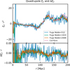 |
Fig. 4 Same as Fig. 3 but for the quadrupole. |
| In the text | |
|
Fig. 5 Angular clustering pseudo-spectrum from exact point-source coordinates and from maps of different resolutions. The lower panel shows the difference with respect to the point-source result. |
| In the text | |
|
Fig. 6 Same as Fig. 5 but for EE shear spectrum. The pseudo-spectra have been scaled by the sky fraction to make them comparable (see main text for explanation). |
| In the text | |
|
Fig. 7 Angular clustering correlation from the direct computation (Nside=2048) or from the power spectrum (ℓmax=8000). The bottom panel shows the difference. The redshift range is z ∈ [1.0, 1.1]. |
| In the text | |
 |
Fig. 8 Same as Fig. 7 but for the angular shear correlation (ξ+, ξ−). |
| In the text | |
|
Fig. 9 CPU cost of RCF computation. We show the CPU cost as a function of pixel resolution Nside, with different redshift resolutions zΔ for clustering (top) or for clustering and shear (bottom). The redshift resolution is, from top down, zΔ=0.0005 (blue), zΔ=0.001 (yellow), zΔ=0.0025 (green), and zΔ=0.005 (red). The dashed lines connect points where Nside and zΔ correspond to the same spatial resolution (from left to right, 6 Mpc, 3 Mpc, 1.5 Mpc). The input data is the full (circles) or the small (triangles) MICE simulation in z = 1.0–1.2. To guide the eye, one node-hour and one node-minute have been indicated by horizontal lines. |
| In the text | |
|
Fig. 10 CPU cost of harmonic-space analysis for 630 redshift-shell pairs. Shown is the cost of computing the redshift–space pseudospectrum for ℓmax=2000–8000 for full (circles) and small (triangles) MICE in z = 1.0–1.2. The redshift resolution was fixed at zΔ=0.005. The squares indicate the cost of constructing the mode-mode coupling kernel to correct for the survey footprint. |
| In the text | |
Current usage metrics show cumulative count of Article Views (full-text article views including HTML views, PDF and ePub downloads, according to the available data) and Abstracts Views on Vision4Press platform.
Data correspond to usage on the plateform after 2015. The current usage metrics is available 48-96 hours after online publication and is updated daily on week days.
Initial download of the metrics may take a while.