| Issue |
A&A
Volume 709, May 2026
|
|
|---|---|---|
| Article Number | A241 | |
| Number of page(s) | 20 | |
| Section | Numerical methods and codes | |
| DOI | https://doi.org/10.1051/0004-6361/202557763 | |
| Published online | 19 May 2026 | |
QUEST: Quasar unsupervised encoder and synthesis tool
A machine-learning framework for generating quasar spectra
1
Hamburger Sternwarte, Universität Hamburg,
Gojenbergsweg 112,
21029
Hamburg,
Germany
2
INAF – Osservatorio Astronomico di Trieste,
Via G.B. Tiepolo, 11,
34143
Trieste,
Italy
3
Department of Astronomy, University of Geneva,
Chemin Pegasi 51,
1290
Versoix,
Switzerland
4
Leiden Observatory, Leiden University,
PO Box 9513,
2300 RA
Leiden,
The Netherlands
5
Department of Physics, University of California,
Santa Barbara,
CA
93106,
USA
6
Institute for Theoretical Physics, Heidelberg University,
Philosophenweg 12,
69120
Heidelberg,
Germany
7
Max-Planck-Institut für Astronomie,
Königstuhl 17,
69117
Heidelberg,
Germany
★ Corresponding author: This email address is being protected from spambots. You need JavaScript enabled to view it.
Received:
20
October
2025
Accepted:
26
February
2026
Abstract
Context. Quasars at the redshift frontier (z > 7.0) are fundamental probes of black hole growth and evolution, but are notoriously difficult to identify. At these redshifts, machine-learning-based selection methods have proven to be efficient, but require appropriate training sets to reach their full potential.
Aims. We present the variational auto-encoder QUEST, which can generate realistic quasar spectra that can be post-processed to generate synthetic photometry and impute spectra.
Methods. We started from the SDSS DR16Q catalogue, pre-processed the spectra, and vetted the sample to obtain a clean dataset. After training the model, we investigated the properties of its latent space to understand whether it has learnt the relevant physics. Furthermore, we provide a pipeline for generating photometry from the sampled spectra, which we compared with actual quasar photometry, and we show the capabilities of the model in reconstructing and extending quasar spectra.
Results. The trained network faithfully reproduces the input spectrum in terms of sample median and variance. By examining the latent space, we found correlations with continuum and bolometric luminosity, black hole mass, redshift, continuum slope, and emission line properties, among others. When we used the network to generate photometry, the results agreed very well with those from the control sample. The model provides satisfactory results in reconstructing emission lines: estimates of the black hole mass from the reconstructed spectra agree well with those from the original SDSS spectra. Furthermore, when spectra with broad absorption line features were reconstructed, the model successfully interpolated over the absorption systems. Compared with previous work, the spectra sampled from our model and the output of their results agree very well. However, QUEST does not require any ad hoc tuning and is capable of reproducing the full variety of spectra available in the training set.
Key words: methods: data analysis / methods: statistical / techniques: photometric / surveys / quasars: general
© The Authors 2026
 Open Access article, published by EDP Sciences, under the terms of the Creative Commons Attribution License (https://creativecommons.org/licenses/by/4.0), which permits unrestricted use, distribution, and reproduction in any medium, provided the original work is properly cited.
This article is published in open access under the Subscribe to Open model. This email address is being protected from spambots. You need JavaScript enabled to view it. to support open access publication.
1 Introduction
Quasars, actively accreting supermassive black holes (SMBHs), are the most luminous active galactic nuclei (AGNs) and non-transient sources in the sky (see Fan et al. 2023, for a recent review). Their luminosity (typically, log (LBOL) ~ 46–48 erg s−1) makes them detectable out to redshift z > 7.5, when the Universe was younger than one billion years (Bañados et al. 2018; Yang et al. 2020; Wang et al. 2021). Their existence places stringent constraints on the growth history and seeding mechanisms of SMBHs (e.g. Yang et al. 2021). Their physical distance allows us to investigate the epoch of reionisation (e.g. Kist et al. 2025) and the chemical and physical state of the intergalactic medium (IGM, e.g. Wang et al. 2020). Quasars shape and affect their surrounding environment: molecular outflows have been detected in samples of quasars at z > 6.0 (Spilker et al. 2025), and feedback from these objects is often invoked to explain galaxy quenching. Quasars themselves are often found to live in overdense regions (Meyer et al. 2022; Wang et al. 2023; Champagne et al. 2023) and are hosted by the most massive (Neeleman et al. 2021) and star-forming (Salvestrini et al. 2025) galaxies in the Universe. Compared to local AGNs, quasars are often found to be overmassive in relation to their host galaxy (e.g. Farina et al. 2022, but see also Li et al. 2022; Silverman et al. 2025). However, despite decades of quasar investigations, many of these topics remain open questions: the main seeding and evolution pathways for growing these objects in such a short amount of time is unclear (see e.g. Inayoshi et al. 2020; Volonteri et al. 2021, for reviews on the topic). A precise timeline for reionisation still eludes us (Ďurovčíková et al. 2024; Qin et al. 2025; Umeda et al. 2026). Although it is well established that quasars and their host galaxy co-evolve (Kormendy & Ho 2013), at z ≳ 6.0, the results of clustering analyses indicate a very diverse environment (see e.g. Meyer et al. 2022; Champagne et al. 2023 and references therein).
In order to effectively investigate these problems, large and well-defined samples of quasars at different redshifts are needed. In the past 20 years in particular, much effort has been devoted to pushing the quasar redshift frontier further into the epoch of reionisation, from redshift z ≈ 6 (Fan et al. 2006) to z ≈ 7.64 (Wang et al. 2021), to characterise the high-z quasar population (Wang et al. 2021). Sensitive near-infrared surveys over wide areas and careful quasar selection techniques were critical to this success. Several methods have been applied in the search for quasars, but most of the known high-redshift quasar population has been identified through standard colour selections (Bañados et al. 2023; Belladitta et al. 2025). However, at z ≳ 7.5, the efficiency of these methods is only about 1% (Nanni et al. 2022), which makes large spectroscopic follow-up campaigns unfeasible for future space-based surveys (e.g. Euclid, Euclid Collaboration 2025, or the Nancy Grace Roman Space Telescope) that will yield a greater number of sources by an order of magnitude than ground-based counterparts.
In preparation for these surveys, statistical methods have been developed and applied with excellent results. Bayesian selection algorithms already yielded the first quasar at z > 7 (Mortlock et al. 2011) and were successfully applied to define complete samples in the VISTA Kilo-degree Infrared Galaxy (VIKING Edge et al. 2013; Barnett et al. 2021) footprint. Although effective, these methods depend on prior assumptions about contaminant populations, which are poorly constrained at faint magnitudes. More recently, machine-learning (ML) techniques have been employed, providing probabilistic classifications of objects and much higher selection efficiencies (≥15%, Wenzl et al. 2021; Nanni et al. 2022; Yang et al. 2024; Kang et al. 2025; Byrne et al. 2024). Nevertheless, a significant limitation still exists: the paucity of training data. Only 11 (including the latest discovery in Matsuoka et al. 2025) quasars with z ≥ 7.0 are currently known. This scarcity can be alleviated by the generation of synthetic datasets, either by parametrising quasar properties and sampling from appropriate distributions (see e.g. McGreer et al. 2021; Temple et al. 2021) or via generative ML approaches. The latter approach offers the advantage of eliminating the need for explicit modelling of quasar properties while potentially capturing previously overlooked correlations.
We present an information maximising variational autoencoder (Info-VAE) trained to produce realistic quasar spectra. These spectra can be post-processed to generate reliable and accurate photometry, which in turn will be used to identify the highest-redshift quasars in upcoming photometric surveys (e.g. the Euclid Wide Survey, the Legacy Survey of Space and Time, and the Roman Wide Survey). Such a model can be naturally extended to several other applications: i) it can reconstruct the quasar continuum in the Lyman-α forest, ii) it can extend quasar spectra to bluer or redder wavelengths, iii) it can reconstruct regions affected by telluric lines or by broad absorption lines (BAL), and iv) ambitiously, it can reconstruct emission lines in order to estimate the quasar black hole mass through single-epoch virial estimators (an approach complementary to previous works, e.g. Eilers et al. 2022, where the BH mass is directly estimated).
The paper is organised as follows: Section 2 details our approach to generating the training datasets and summarises the most relevant information. Section 3.1 provides a general introduction to VAEs, describes our implementation, and outlines our strategy to optimise the hyperparameters. In Section 4 we examine the properties of the latent space and assess whether the model has learnt relevant quasar physics. Section 5 presents various use cases for the Info-VAE, demonstrating its capabilities. We compare our results with those from previous studies and discuss the known limitations in Section 6, and we conclude in Section 7. We adopted the following cosmological parameters:
Ωm = 0.315, ΩΛ = 0.685, and h = 0.674 (Planck Collaboration VI 2020). All magnitudes are presented in the AB system (Oke & Gunn 1983).
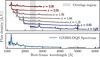 |
Fig. 1 Top panel: example of SDSS spectra at different redshifts included in the GP dataset. Bottom panel: example of a spectrum from the GNIRS-DQS survey, highlighting the extended coverage at redder wavelengths. The spectral gaps are are due to telluric absorptions. |
2 Training datasets
In this section, we describe the datasets we used to train the Info-VAEs. We assembled three datasets and used them to train three different models with the same network architecture. All datasets were processed uniformly and differed only in terms of the minimum signal-to-noise ratio and wavelength coverage required. Each dataset was used to train the corresponding VAE model (see Sect. 3.2). In the following, we refer to these datasets and the corresponding models as general purpose (GP), full overlap blue (FOB), and full overlap red (FOR) datasets.
2.1 The general purpose dataset
We aim to train a ML model capable of several tasks: (i) generating realistic quasar spectra and photometry, (ii) inputting a quasar spectrum to regions that were not originally covered by the SDSS spectrograph, (iii) reconstructing intermediate regions of the quasar spectrum that are contaminated by BALs or affected by instrumental and observational systematics, and (iv) faithfully reconstructing selected emission lines and allow, for example, computation of the quasar's black hole mass.
To be able to perform these tasks, we require a model capable of generating spectra that cover a large (rest-frame) wavelength range. For the purpose of this paper, this is chosen to be between 980 Å and 5500 Å, to cover the entirety of the Lyman-β forest, and UV and optical emission lines up to the Hβ–O [III] complex. Unfortunately, no large spectroscopic survey provides data that fully covers this range. However, it is possible to assemble a dataset in which spectra at different redshifts contribute to different portions of this wavelength space. In the case of the SDSS, for example, low-z spectra cover the reddest wavelengths we require, while higher-z spectra cover the bluest ones (Fig. 1). In addition to this, it is possible to combine spectra of the same object, collected with different facilities, to cover a larger wavelength range. In order to assemble an optimal training set, we started from the SDSS DR16 quasar catalogue (Lyke et al. 2020, hereafter DR16Q). We opted for a mature and well-studied sample, rather than more recent ones (e.g. the first data release from the DESI Collaboration DESI Collaboration 2025). This allowed us to exploit ancillary data made available by the community (e. g. Wu & Shen 2022), and complement and extend SDSS spectra to redder wavelengths including publicly available near-infrared data from the GNIRS-DQS survey (Matthews et al. 2021, 2023). These spectra were independently re-reduced and used as dropin replacements for the corresponding SDSS spectra, resulting in the replacement of ~100 of them. Additional details about the data reduction will be presented in a forthcoming publication (Yang et al., in prep.). As a first step, we collected all spectra that satisfy simple quality cuts1:
0.59 < Z_PIPE < 2.77 and ZWARNING = 0, to select reliable redshifts and guarantee that, taken together, the spectra fully cover the aforementioned wavelength range while allowing a common overlap region between 2300–2600 Å. Although the wavelength range over which we require the overlap is arbitrary, it is important to include at least an emission linefree region to consistently normalise all inputs. We choose the normalisation region to be between 2350 Å and 2360 Å (rest-frame wavelength);
BI_CIV ≤ 0 and BI_SiIV ≤ 0, to remove quasars with the most prominent BAL features;
SN_MEDIAN_ALL2 > 15 and M_I < −20, to only include spectra of bright quasars with sufficient S/N to clearly detect continuum, emission lines, and weaker BAL features. We note that the combination of these two requirements implicitly biases the training sample towards the brightest SDSS quasars at each given redshift.
This resulted in a parent sample that contains 20 007 quasars, with a median redshift of 1.62 and absolute i-band magnitude −26.82. Once collected, all the spectra that satisfied these simple cuts were further preprocessed and analysed to discard those with artefacts, large interpolated regions, and weaker BALs features that were not excluded by the balinicity index cut previously imposed. In particular, we further cleaned up the sample by identifying and excluding spectra with at least fifteen consecutive interpolated pixels, without any flux density value in the normalisation window, or for which the median S/N in the normalisation window is lower than seven. Furthermore, we excluded reddened spectra, spectra with broad absorption features on the blue or red side of the Lyman-a and C IV emission lines via a custom automated pipeline, and spectra with fewer than 100 valid pixels. We show examples of rejected spectra in Fig. 2. The cleaning procedure excluded 1786 spectra, leaving us with a dataset of 18 221 objects that we deemed usable for training. For all these spectra, we:
shifted them to the respective rest frame, by dividing the wavelength axis and multiplying the quasar flux density by (1 + zquasar). We used Z_PIPE as the fiducial quasar redshift;
corrected for the effect of the Milky Way's dust extinction by de-reddening each spectrum using the Gordon et al. (2023) A(λ) extinction curve (see also Gordon et al. 2009; Fitzpatrick et al. 2019; Gordon et al. 2021; Decleir et al. 2022, for individual contributions to the model). We assumed an average value R(V) = 3.1, as is commonly done for the Milky Way (see e.g. Whittet & van Breda 1980; Fitzpatrick & Massa 1999) and computed the E(B – V) at the quasar coordinates (l, b)quasars based on the two dimensional dust map from Chiang (2023);
fitted a continuum to the quasar spectrum, following an approach similar to that adopted in Bosman et al. (2021), developed by Young et al. (1979); Carswell et al. (1982), and first implemented in Dall'Aglio et al. (2008). Briefly, the algorithm fits a spline over equally spaced nodes along the quasar spectrum. During the fitting, individual pixels are iteratively masked via asymmetric sigma-clipping. Iterations are stopped, and convergence is reached, when the standard deviation of the fluxes in the retained pixels is less than the average observed noise. The fitted continuum was used to further clean up the sample to remove weak BALs and replace the Lyman forest of the spectrum with unabsorbed flux (see below).
normalised each spectrum by dividing the flux density by the median flux density in a wavelength region between 2350–2360 Å.
As a final step, we resampled all the spectra on a common wavelength grid, from 980 Å to 5500 Å, linearly spaced in velocity space. We set the pixel size to 140 km s−1. For all high-z spectra we replaced the Lyman-a forest with the fitted continuum, smoothly joining the latter with the original spectrum around 1225 Å. This step is necessary: for instance, to generate synthetic photometry of quasars with z ≳ 2.0, the suppression of the flux blueward of the Lyman-a due to the intergalactic medium should be computed on the basis of the unabsorbed continuum.
The sample used for training has a median redshift of 1.61 (16th–84th percentiles: 0.95–2.27, respectively) and median absolute i-band magnitude of −26.79, (16th–84th percentiles: −27.73 – −25.47, respectively). We show a density plot with the distribution in the z–Mi plane in Fig. 3, and a composite spectrum of all quasars that meet the selection criteria in Fig. 4. We provide the complete median composite of our training data in Table A.1.
In the same figure, we also plot the type-I quasar template from Vanden Berk et al. (2001) with the solid red line (top panel) and the type-I quasar template from Selsing et al. (2016) with the solid purple line (middle panel). The median spectrum and the templates agree very well redward of the Lyman-α emission line; the continuum in the Lyman-α forest is instead higher in our median spectrum, as a consequence of the grafting of the fitted continuum (see below). Around 5000 Å, the Selsing et al. (2016) template shows better agreement with the median input spectrum, whereas emission lines are matched equally well. This suggests that, even if the training sample is biased towards bright quasars, it is not solely representative of the very bright end of the population.
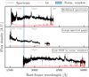 |
Fig. 2 Examples of rejected spectra, and the cause of rejection. The black line shows the original SDSS spectrum, the red line shows the nominal uncertainty, and the light grey line shows the zero-flux level. |
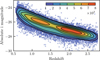 |
Fig. 3 Density plot showing the redshift-absolute i-band magnitude distribution for the spectra that meet the selection criteria. The colour map shows the number of spectra in each contour line. |
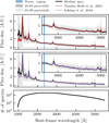 |
Fig. 4 Median spectrum and logarithmic number of spectra contributing to the median in each pixel. Top panel: Median spectrum of the quasars included in the training set (thick solid black line) compared to the Vanden Berk et al. (2001) (thin solid red line). The shaded regions represent the 16th–84th percentiles (dark grey) and the 1st–99th percentile (light grey). The vertical blue band represents the region in which we computed the normalisation factor for each spectrum. Middle panel: Same as the top panel, but for the Selsing et al. (2016) composite spectrum. Bottom panel: Logarithmic number of spectra contributing to each pixel in the median spectrum. By construction, all spectra contribute to the region between 2300–2600 Å. |
Summary of the most relevant information for each dataset.
2.2 The full overlap blue and full overlap red datasets
We followed the same approach as outlined in the previous section to prepare these datasets. In both cases, we started from the SDSS DR16Q, selected quasars that meet basic quality cuts, and processed the sample. We lowered the S/N threshold to 5 and required full coverage of the wavelengths 1175–2950 Å (FOB) and 2300–5500 Å (FOR). Although suboptimal, lowering the S/N threshold was needed because of the lower number of spectra available, which turned out to be insufficient to train the VAE. We summarise the most important information for the three datasets in Table 1, including the total number of sources, the overlap range we required, and the median redshift and absolute i-band magnitude.
3 Design of the Info-VAE for QSO spectra
In the section we provide a general introduction to variational auto-encoders, describe the architecture of QUEST, and the training strategy we adopt. We also outline the differences between "classic" VAEs and Info-VAEs, of which QUEST is an example.
3.1 Variational auto-encoders
Variational Auto-Encoders (VAEs, Kingma & Welling 2013) are unsupervised generative networks that map, in a probabilistic manner, high-dimensional data to a lower-dimensional representation. This low-dimensional representation, with dimension 𝒟, is generally referred to as a latent space and, by design, should reflect the most meaningful properties of the data.
From an architecture point of view, a VAE is similar to a standard auto-encoder (AE, Rumelhart & McClelland 1987) and consists of two networks chained together: an encoder that compresses the data and performs (non-)linear dimensionality reduction, and a decoder that takes samples from the latent space distributions and reconstructs them to the higher-dimensional input representation. The key difference from an AE is in the interpretation of the latent representation z of a given input x: in a VAE, this is a probability distribution function p(z|x); in an AE, it is instead a single point. In principle, this distribution could assume any form. In practice, however, it is generally assumed to be a multivariate Gaussian, that is p(z|x) ~ 𝒩(μ, σ), where μ and σ are the output of the encoder and represent the means and standard deviations of the Gaussian distributions describing each latent space dimension. μ and σ are the key ingredients in building the latent space dimensions zi using the reparametrisation trick: z = μ + єσ, with є ~ 𝒩(0,1). Finally, the decoder takes the latent space as input and returns a distribution of reconstructed outputs x′.
In order to train the algorithm, one needs to define an objective function to minimise. In the standard VAE implementation, this is taken to be the evidence lower bound (ELBO). The ELBO is the sum of two loss terms: a reconstruction and a regularisation loss. The former encourages the network to accurately reconstruct the input data. The latter, on the other hand, encourages the latent space to match the chosen distribution p(z|x) as accurately as possible. In the case where p(z|x) is given by independent unit Gaussians, the regularisation term also encourages disentanglement (i.e. uncorrelated latent variables). The standard formulation of the ELBO is
 (1)
(1)
with β = 1 and KL representing the Kullback–Leibler (KL Kullback & Leibler 1951) divergence between the latent distribution p and the prior q.
Several variations of this standard picture have been proposed in order to address issues with the classic VAE implementation. Examples include β-VAEs (Higgins et al. 2017, where β ≠ 1) and InfoVAEs (Zhao et al. 2017), which we employ here. Two main reasons motivated the introduction of the InfoVAE: on the one hand, the regularisation part of the loss function can be too strong with respect to the reconstruction; on the other, ELBO-based VAEs tend to overfit the data if the training dataset is not sufficiently large. In practice, both issues result in a VAE that does not learn a meaningful representation of the data either because the algorithm simply produces q(z) regardless of the input or because it overfits the data without actually learning the underlying distribution. An InfoVAE addresses this issue by modifying the loss and including an additional term,
 (2)
(2)
where MMD represents the Maximum Mean Discrepancy (MMD, Gretton et al. 2012), computed between each latent space dimension z and the prior q(z). This new loss addresses both issues: on the one hand, the strength of the regularisation term can be lowered, tailored to specific applications, or removed altogether. The additional regularisation term, based on the MMD, encourages a better use of the latent space and has been shown to be significantly less prone to overfitting (Zhao et al. 2017).
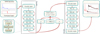 |
Fig. 5 Schematic representation of the model architecture, input, and output. The network receives as input the concatenation of an SDSS spectrum, normalised by the median spectrum, and the coverage mask (top left panel). It then encodes the input to produce a latent space representation Z, that is decoded to produce a new spectrum (top right panel). The new spectrum (shown in red) covers a wider wavelength range compared to the corresponding input (shown in black) and is generally less noisy. The encoder and decoder are built as the reverse of each other by combining several hidden layers, denoted in the schematic by HL followed by the corresponding output dimension. Each hidden layer is a combination of a linear layer, followed by a BatchNormlD layer, and the activation function (bottom left). |
3.2 Model architecture, training strategy, and hyperparameters
A schematic representation of our InfoVAE architecture is shown in Fig. 5. We employed a symmetric architecture, in which the encoder and decoder mirror each other. The network receives as input the concatenation of the preprocessed spectra (divided by the median spectrum, as we found this to make the training more stable) and the respective coverage mask, added to explicitly inform the network about the wavelength range covered by each spectrum, and whether a given pixel should be ignored for any reason. The concatenation is passed through a series of hidden blocks to produce two vectors, μ and σ. Through the reparametrisation trick, these are encoded in the latent space 𝒵 and finally decoded to produce the reconstructed spectrum. Each hidden block is constituted by a linear, fully connected layer followed by batch normalisation and the activation function. We opted for the activation function proposed by Alsing et al. (2020), which we found to outperform the widely used LeakyReLu (Leaky Rectifier Linear unit, Maas 2013). The network was implemented in PyTorch (version 2.7 Ansel et al. 2024) and trained using the Adam optimiser (Kingma & Ba 2017). The reconstruction loss is defined as the χ2 statistic between the reconstructed and corresponding input spectra, computed using the formal SDSS inverse variance. This has the advantage of naturally taking into account the uncertainty in the training data, which would otherwise be ignored. We followed the standard InfoVAE implementation for the regularisation term, but set α = 0 in Eq. (2), following the recommendation of Zhao et al. (2017). We identified the optimal λ by hyperparameter optimisation (Table 2).
To limit overfitting, at run-time, we randomly masked out part of the spectra before feeding them as input to the encoder. This mask was not considered when computing the reconstruction loss. This strategy is commonly employed in denoising AEs to encourage the model to learn intrinsic and robust properties of the population. We used a batch size of 128 and trained the network for 5000 epochs, but implemented an early stopping strategy to interrupt the process if the validation loss did not improve for more than 200 consecutive epochs. The training and validation losses for the GP network are shown in Fig. 7, as a function of the latent dimension. It is evident that employing a number of latent dimensions larger than ten does not improve the validation loss. We used this to limit the grid of parameters we searched in the optimisation step. To optimise the hyperparameters of the network, we selected a limited subset of them, listed in Table 2, and performed a systematic grid search. We did not vary all possible parameters and did not change the architecture in order to keep the run-time of test runs manageable. We selected the best network as the one that provided the best reconstruction. We adopted the same architecture, and optimised the hyperparameters in the same way, for all training sets.
The output of the "best" model for the GP dataset is shown in Fig. 6 (and the equivalent for the FOR and FOB datasets in Fig. B.1). The parameters used to train the best model are listed in Table 3. Here, we sample spectra from the InfoVAE and compare them with the input data. In particular, we show with the solid black line the median input spectrum and with the solid grey line the median sampled spectrum. The dashed black line encloses the 16th–84th percentile of the input data, whereas the grey-shaded area the 16th–84th percentile of the sampled spectra. All models show excellent agreement with the input data in terms of median spectrum and variance. The emission lines are faithfully reproduced, as is the quasar continuum. The variance is reduced to almost zero at ~2350 Å: this is expected, as it is the window in which we normalise the spectra.
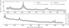 |
Fig. 6 Sampled spectra from the GP model compared to the input spectra. In both panels, the solid and dashed black lines indicate the median, 16th, and 84th percentile of the input data respectively. The solid grey line represents the median spectrum of 10 000 realisations sampled from the VAE, while the shaded area encompasses the 16th and 84th percentile of the same sampled data. The model is able to accurately reproduce the median and the variance of the input spectra. We note that all spectra are normalised using the flux between 2350 Å and 2360 Å as reference. The comparison between median sampled spectrum and median input for the FOR and FOB models is shown in Fig. B.1. |
Parameters optimised as part of the grid search.
Parameters used to train the best model after the optimisation procedure.
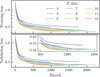 |
Fig. 7 Training and validation losses for the GP network as a function of the number of latent dimension. |
4 Latent space exploration
After training each model, we explored the properties of the latent space to understand whether the latent dimensions reflect a particular (or a combination of) quasar physical properties. We employed exploratory and well-established methods, and we focused our analysis on the GP model. We first explored the latent space variations through visual inspection, varying one latent space dimension at a time while keeping the others constant. We then decoded each mock latent space representation and observed the effect of each latent on the reconstructed spectrum. Secondly, we applied an unsupervised dimensionality reduction algorithm (Uniform Manifold Approximation and Projection for Dimension Reduction, hereafter UMAP, McInnes et al. 2018) to the latent space, projecting it onto a two-dimensional embedding. We then colour-coded the representation and looked for trends and clusters. Finally, we computed the Mutual Information (MI Shannon 1948) between each latent space dimension and selected physical properties of the SDSS quasars derived in Wu & Shen (2022). To do so, we employed GMM-MI (Piras et al. 2023), a Gaussian mixture model estimator for MI.
4.1 Latent space variations
We initially adopted an exploratory approach to investigate whether our latent space correlates with any physical quasar property. We started by encoding the full training dataset and obtained its latent space representation. By exploiting the fact that our latent dimensions are approximately Gaussian (or, equivalently, that the mean and median of each dimension are approximately zero, see Fig. C.1), we generated a "baseline" latent space, where each sample is represented by a vector of zeros. We expect this latent space to be close to the median quasar spectrum used to train the model (Fig. 4). From this "baseline" latent space, we varied each latent space dimension between the respective first and 99th percentiles while keeping the other dimensions fixed at zero. We then decoded the mock latent space and plotted the resulting spectra. The results, for the five latent space dimensions that produce the largest variation, are shown in Fig. 8; the remaining are presented in Fig. D.1. However, we emphasise that unlike methods such as Principal Component Analysis (PCA), the cardinality of the latent dimensions does not correlate with the amount of available information: for example, LD1 does not necessarily contain more information than the other latent dimensions. Moreover, each dimension does not capture a single spectral feature, but rather a combination of several. For example, there is a clear correlation with emission line strength (LD2, LD8, LD10, and to some extent LD5), the continuum slope (LD11), or the Fe II emission complex and pseudo-continuum (LD2, LD5). Emission line variations are not uniform, with some latent dimensions more evidently affecting rest frame UV or optical lines: for example, in LD10 there are significant changes in C IV and Mg II, which are not reflected in the H-β line.
4.2 UMAP dimensionality reduction of the latent space
A more robust approach to interpreting the latent space of a VAE is to further reduce its dimensionality through dimensionality reduction algorithms, such as UMAP. UMAP is an unsupervised and non-linear dimensionality reduction algorithm that attempts to learn the manifold structure of the data it is applied on. It produces a low-dimensional embedding that preserves the essential topological structure of that manifold (McInnes et al. 2018). Intuitively, UMAP first creates a topologically equivalent, high-dimensional representation of the data, then optimises a low-dimensional equivalent to match it, using cross-entropy as a measure of similarity. UMAP uses randomness in computing the embedding: as a consequence, the distance between clusters or the absolute values associated with each embedding point are meaningless and not deterministic. Instead, the focus should be on the resulting clusters, which reflect actual patterns in the data.
We started from the same latent space representation obtained in the previous step and preprocessed it to scale all dimensions using a RobustScaler from scikit-learn. We then fitted a UMAP model to the scaled latent space representation and obtained a two-dimensional embedding of our 𝒵. We kept all UMAP parameters at their default values, with the exception of n_neighbors (set to 15) and mid_dist (set to 0.01). We determined these values through trial and error: the embedding results did not significantly depend on the choice of hyperparameters as long as n_neighbors was not too large (≳50). Finally, for visualisation purposes and qualitative analysis, we applied a clustering algorithm (HDBScan, McInnes et al. 2017) to automatically identify clusters in the UMAP embedding. We show the results in Fig. 9. The UMAP embedding features a smooth and large cluster ("main", orange), two small clusters (blue and green), and an extended tail (red). This reflects the homogeneity of the training set, designed to be as clean as possible of reddened spectra, spectra with BALs, and artefacts. As shown by each median spectrum in the bottom panel of Fig. 9, spectra belonging to the "main" cluster are the closest to typical type-I quasars. Spectra belonging to the red "tail" are redder than the typical quasar and exclusively at low-z, whereas those in the blue cluster appear bluer than the average. Finally, spectra belonging to the green clusters lack most of the typical quasar emission lines. This could indicate that the VAE has learnt to recognise blazars, spectra misclassified as quasars, or spectra with an incorrect redshift. We visually inspected each of them (twenty in total), noting that 75% do not show prominent emission lines, while the remaining ones had not been assigned the correct redshift. These objects show the power of the VAE as a tool for identifying outliers and errors in large catalogues. They will be removed in the future from all datasets.
Furthermore, we plot the resulting UMAP embedding and colour-code each point according to selected quasar properties derived in Wu & Shen (2022). The results are shown in Figure 10. The S/N and the galactic reddening are not correlated with the UMAP embedding: this implies that the model did not learn the noise pattern of the SDSS spectra and that the de-reddening applied during the preprocessing successfully removed the effect of galactic extinction. Instead, there is a strong gradient in redshift and absolute i-band magnitude. This trend can be attributed either to the addition of the coverage mask as input to the model, or to selection effects inherited from the training set (that is, a combination of selection effects from the SDSS survey, combined with the S/N requirement we impose (Fig. 3), or to a combination of the two. We colour-code the last panel by the logarithm of the Eddington ratio, to check whether the model has learnt a physically meaningful quantity. The result hints towards a positive answer, as it is possible to identify regions of the embedding where quasars with high or low Eddington ratios are grouped together.
Finally, we investigated how the reconstruction changes as a function of the coordinate in the UMAP embedding. To do so, we employed the inverse_transform method implemented in UMAP and followed the bolometric luminosity trend as illustrated in Fig. 11. We arbitrarily placed 13 points (coloured circles, left panel) following the change in bolometric luminosity. We then obtained the corresponding points in the latent space by applying the inverse UMAP transformation, decoded them into spectra, and plotted them stacked on top of each other (right panel). Several interesting trends appear. It is immediately noticeable that sampling from the region with the highest bolometric luminosity produces quasars with the weakest emission lines: this indicates that the VAE has learnt the Baldwin effect (Baldwin 1977). In addition, quasars with higher bolo-metric luminosity produce broader lines: this is consistent with our expectations of them having larger black hole masses. Furthermore, we checked whether the peak of the most prominent emission line shifts as a function of the bolometric luminosity. Surprisingly, the peak position of Mg II evolves redward with redshift, whereas the C IV does not evolve at all. Both behaviours are unexpected: previous works identified a correlation between luminosity (see e.g. Schindler et al. 2020) and C IV blueshift that is not observed in Mg II. A possible explanation is a systematic issue in the SDSS redshift pipeline for spectra in which only rest-frame UV emission lines are available. In these cases, blue-shifted C IV emission could lead to an underestimated redshift estimate, in turn causing a redshifted Mg II line.
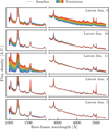 |
Fig. 8 Decoded spectra obtained from a mock latent space, where we varied a single latent dimension (indicated in the top right corner) while keeping the others constant. In order to better visualise the results we use a different scale for the blue and red side of the decoded spectra; the two, however, smoothly join. We show in this figure the five latent space dimensions that produce the largest variations and in Fig. D.1 all the latent dimensions. |
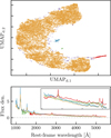 |
Fig. 9 Two-dimensional UMAP embedding of the VAE latent space for the GP model. Top panel: Clusters identified in the embedding, highlighted using different colours (orange, green, and red). Outliers (i.e. points that are not associated with any cluster) are shown in purple. For visualisation purposes, the bottom panel shows the median SDSS input spectrum for objects in each cluster, with matching colour-coding. |
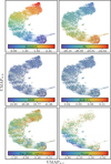 |
Fig. 10 UMAP embedding colour-coded by redshift, absolute i-band magnitude, S/N, galactic extinction, logarithm of the Eddington ratio, and continuum slope (top to bottom, left to right). |
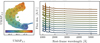 |
Fig. 11 UMAP representation colour-coded as a function of the bolometric luminosity and the resulting spectra decoded from the latent space point in the direction of evolution. Left panel: UMAP embedding; the points on which we applied the inverse UMAP transformation are highlighted as scatter points and are colour-coded using the average neighbouring colour. Right panel: Spectra decoded from latent space samples highlighted in the left panel and colour-coded according to the respective originating scatter point. |
4.3 Mutual information
To quantitatively measure the correlation between latent space dimensions and quasar physical properties, we computed the Mutual Information between each latent space dimension and selected quasar properties, again obtained from Wu & Shen (2022). The MI is a measure of the mutual dependence between two random variables X and Y. It captures linear and non-linear correlation between X and Y and is defined in terms of the Kullback-Leibler divergence DKL,
 (3)
(3)
with (X, Y) being a pair of random variables defined over a space 𝒳×𝒴, P(X,Y) their joint distribution and PX, PY their marginal distributions, and ⊗ denoting the outer product between the two marginal distributions. MI is, by definition, non-negative and equal to zero only when X and Y are completely independent. If X and Y are continuous random variables, then MI can be written as
 (4)
(4)
with P(X,Y) representing the joint probability density function of X and Y, and PX and PY the respective marginal probability density functions. MI is expressed in "nat" (natural unit of information) when taking the natural logarithm of the ratio, as is in Eq. (4). Several methods have been proposed to compute the MI between two random variables, including histograms and Gaussian mixture models. We used the publicly available GMM-MI Python package (Piras et al. 2023), which estimates the probability density functions using Gaussian mixture models, and has the added benefit of providing uncertainties through bootstrap resampling. The algorithm was designed and applied in the past to interpret the latent space of deep learning models (Lucie-Smith et al. 2024; Lucie-Smith et al. 2024). A detailed discussion of GMM-MI is beyond the scope of this paper, and we refer to Piras et al. (2023) for a thorough description.
We present the results of mutual information analysis in Fig. 12, where we show the ten most correlated properties and the corresponding mutual information values for each latent dimension (with the exception of LD3 and LD9, excluded due to their minimal correlations). As discussed in Sect. 4.1, most latent dimensions correlate with several variables. LD5, in particular, strongly correlates with bolometric luminosity, BH mass, continuum luminosity, and Mi. As noted in Sect. 4.2, these correlations probably originate from the selection function of the training dataset. LD2, on the other hand, correlates with emission line properties, as do LD1 and LD6. Most dimensions also show a significant correlation with redshift and with the continuum slope, particularly LD11, consistent with our findings from Figs. 8 and 10.
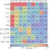 |
Fig. 12 Mutual information between all the latent dimensions of the GP model and the ten most correlated variables. |
5 Applications
In this section, we show the capabilities of the trained VAE models to perform a variety of tasks, from generating quasar photometry to reconstructing quasar emission lines in order to compute their black hole masses. In all cases, we will use the "best" model trained on a specific dataset, where "best" is defined as in Sect. 3.2.
5.1 Generation of synthetic quasar photometry
The most straightforward application of the GP model (and the initial goal that motivated the development of this InfoVAE) is the generation of quasar photometry, given a redshift range [zmin, zmax] and a reference absolute magnitude range [M1450,min,M1450,max]. For this application, the GP model is optimal, featuring the largest wavelength coverage, thus allowing the most flexibility in generating photometry in different filters.
We started by sampling the latent space and generating synthetic quasar spectra. They cover the rest-UV and optical wavelength range from 980 Å to 5500 Å. We did not bias the sampling towards any quasar spectral property besides those that originate from the training set. Because of this, the sampling naturally reflects the diversity in spectral shapes of the (bright) SDSS quasars included in the training sample, without the need to explicitly model them. Although realistic in terms of spectral shape, the examples generated by the VAE are scaled to arbitrary units and at redshift z = 0: as such, they need to be preprocessed before being suitable for the generation of photometric data.
We first defined a reference redshift [zmin, zmax] and absolute magnitude [M1450,min, M1450,max] interval, together with thenumber of quasars to generate. Given these priors, we sampled the z–M1450 space and produced tuples (zi, M1450,i). The sampling can be either uniform, according to a user-defined quasar luminosity function, or based on an empirical distribution estimated from user-provided data. We then smoothly joined the Lusso et al. (2015, Table 1 in the paper) quasar template with the generated spectra. First, we defined an overlap range of 980 Å and 1020 Å. Then, we rescaled the Lusso et al. (2015) template so that it matched the quasar pseudo-flux in this wavelength window. Finally, we smoothly joined the template and the sampled spectrum.
We then associated to each zi, M1450,i pair a quasar spectrum. Each spectrum is shifted to the assigned redshift by multiplying the wavelength axis by (1 + zi), and scaled to the respective M1450 by first computing the apparent magnitude m1450,i = M1450,i + DistMod + Kcorr, where DistMod represents the distance modulus computed using the standard Planck Collaboration VI (2020) cosmology and Kcorr = 2.5log10(1 + zi). We reddened each spectrum using the same reddening model employed during the generation of each training dataset (Gordon et al. 2023, see Sect. 2.1)). To do so, we generated galactic coordinates (l, b) by uniformly sampling l between 0° and 360°, and b between -90° and +90°, ensuring |b| > 15° for consistency with the training dataset. Finally, we used SimQSO (McGreer et al. 2021) to generate random realisations of IGM absorption spectra. We multiplied these by each sampled quasar spectrum to simulate the effect of the Lyman forest and depress the flux blue-wards of the Lyman-α emission line. This completeed the preprocessing steps. To estimate photometry from the spectra, we used SpecLite (Kirkby et al. 2024). SpecLite convolves each spectrum with the appropriate filter response curve to obtain AB magnitudes. These AB magnitudes are uncertainty-free and do not take into account the photometric depth of the survey. To account for this, we perturbed the photometry under the assumption that, for each photometric band b and apparent magnitude bin Δm, the original survey error distribution is approximately Gaussian. We verified this approximation to be reasonable and estimated the error function σ(Δm) (that is, the typical uncertainty as a function of apparent magnitude). Then, for each apparent magnitude m, we assigned an uncertainty σ using the error function and sampled a new perturbed magnitude mσ from a Gaussian N(m, σ). These mσs, together with the associated uncertainties, represent the final product of the algorithm.
As a first sanity check, we compared our synthetic photometry against the SDSS DR16Q quasar photometry. We computed the error function as outlined in the previous section, by selecting SDSS point sources. We generated the redshift-absolute magnitude grid by sampling the corresponding distributions of the SDSS DR16Q catalogue3. The results are shown in Fig. 13, where, as a function of redshift, we show the median flux ratio from the entire SDSS DR16Q with the dashed dark red line and with the solid black line the median synthetic photometry. The red (blue) shaded area represents the 16th and 84th percentile range for the entire SDSS DR16Q (for the quasar part of the training dataset). We show the same quantities for the synthetic photometry using the dashed, black lines. In addition to the ugriz SDSS photometry, we also include the UKIRT Infrared Deep Sky Survey (UKIDDS) Y, J, H, and K data. Our generated spectra do not fully cover the H and K bands at redshift z ≲ 3, and as such we do not include the photometry of Fig. 13. The median SDSS, UKIDSS, and synthetic photometry agree well in most cases, with some minor differences in the u–g colour. This could be attributed to different factors: on the one hand, our reconstruction of the unabsorbed continuum blueward of the Lyman-a forest could be imperfect; on the other hand, the IGM model we employ (McGreer et al. 2021) is not fully representative of the IGM at these redshifts. Moreover, in the case of the UKIDSS bands, the spread in quasar colours does not match the SDSS data. This is likely a consequence of the censored training dataset that we are using and it is evident from the blue shaded area, which shows a consistently narrower spread in the training quasar colours. The narrower spread we observe reflects a bias towards the brightest quasars at each given redshift (see Sect. 2.1) and also the presence of non-type-I quasars in the DR16Q catalogue.
In addition, to confirm that the model provides accurate photometry also in the highest-redshift regime, we compare the synthetic photometry with that of the z > 5.3 quasar catalogue provided by (Fan et al. 2023). We crossmatched the catalogue against the Panoramic Survey Telescope and Rapid Response System survey (PanSTARRS Chambers et al. 2016), the UKIRT Infrared Deep Sky Survey (UKIDSS Lawrence et al. 2007), the VISTA Kilo-Degree Infrared Galaxy survey (VIKING Edge et al. 2013) and the Vista Hemisphere Survey (VHS DR5 McMahon et al. 2013) using a 0.5 arcsecond radius. The results are shown in Fig. 14: as in the lower redshift regime, the model faithfully reproduces the quasar colours.
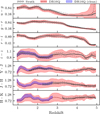 |
Fig. 13 SDSS and UKIDSS colours as a function of redshift for the SDSS quasar and our synthetic photometry. The model faithfully reproduces the SDSS median colour at all redshifts, with the exception of the u–g colour, where the absorption from the IGM and the interpolation over the Lyman forest significantly affects the u band. The same happens for UKIDSS colours, albeit with a narrower spread. |
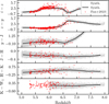 |
Fig. 14 Same as Fig. 13, but for the high-z sample from (Fan et al. 2023). In this case, we represent the photometry from the real quasars with scatter points instead of presenting the 16th–84th percentile range due to the low number of high redshift quasars. |
5.2 Reconstruction of spectra with BAL features
A second application for the model is the reconstruction of BAL absorption features in quasar spectra. Existing methods (see e.g. Rankine et al. 2020; Choi et al. 2022) use PCA or mean-field independent component analysis (MFICA) to reconstruct the unabsorbed quasar continuum, with reported accuracies of up to 93% (Rankine et al. 2020). Qualitatively, we expected QUEST to be capable of interpolating over the absorption features and produce a faithful reconstruction of the underlying continuum. However, because it has not been optimised for this task, we did not expect it to match the performance of other methods optimised for this problem. We employed the FOB model to carry out this test and we proceeded as follows: starting from the 12th data release of the SDSS quasar catalogue Pâris et al. (2017), we downloaded the BAL quasar subset4. Then, we selected the quasars that satisfy the wavelength coverage conditions used to generate the FOB dataset. This is not necessary, as the model is capable of extending the spectra to bluer or redder wavelengths, but it provides a well-defined dataset of nine objects. In addition, it represents a "best-case" scenario, where the model has access to spectra covering the full wavelength range. We visually inspected the spectra, manually masked the absorption systems, and fed the masked spectra to the model for reconstruction. Qualitatively, the model reconstructs the unabsorbed continuum to a good degree of accuracy, interpolating over the absorption features, and returning an unabsorbed continuum that closely matches the input spectra in most of the cases. However, the model struggles to reconstruct the emission lines, in particular the Lyman-a, which appears to be often underestimated in the reconstruction. Moreover, most of the spectra available for the reconstruction appear to feature blue-shifted components and asymmetric emission lines that the model struggles to reproduce faithfully (see e.g. the middle panel in Fig. 15). This is hardly surprising, as it is trained on a "clean" dataset, devoid of spectra with similar features. Finally, in some cases, the model underestimates the unabsorbed continuum (see again e.g. the middle panel in Fig. 15). The reason for this is currently unclear, but a detailed exploration is beyond the scope of this paper.
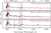 |
Fig. 15 Example of a spectrum with an acceptable reconstruction (top panel), a spectrum for which the model underestimates the Lyman-α and N V complex (middle panel), and a spectrum for which instead the restframe UV and optical emission lines are not well reproduced (bottom panel). We show in black the input spectrum, in red the reconstruction, and with the shaded grey areas the masked out regions. We show the remaining spectra in Fig. F.1. |
5.3 Black hole mass from reconstructed emission lines
In addition to BAL quasar reconstruction, we further explored the imputation capabilities of the VAE (and, in particular, of the FOR model) and used it to reconstruct the Mg II and H-β emission lines of selected SDSS quasars. To validate the reconstruction, we then fitted the reconstructed spectra and computed the black hole mass using well established single epoch virial estimators. We finally compared the estimates with each other and with the same estimate obtained by fitting the original SDSS spectra following the approach presented in Wu & Shen (2022).
In order to ensure that the test is as unbiased as possible, we only considered legacy SDSS quasars, not included in the training set. These represent the most similar but independent dataset to the spectra we used to train the algorithm. We prepared a dataset containing these spectra using the same approach outlined in Sect. 2.1. In addition, we tested different scenarios: before feeding the spectra to the VAE to reconstruct them, we either did not mask any emission line, masked only the Mg II or the H-β emission line, or both. This served as an additional test to check whether the model utilises information from either emission lines to compensate for the lack of the other, or if continuum information are sufficient. To be consistent with the results presented in Wu & Shen (2022) and allow a direct comparison, we followed the same procedure and used the same input files described in their work. We present here a brief summary of the most significant steps and refer to the original paper for additional details. All spectra were automatically modelled using PyQSOFit (Guo et al. 2018; Shen et al. 2019). The model includes a continuum (modelled as a power law with the addition of a third-order polynomial), optical and UV Fe II emission using empirical templates (Boroson & Green 1992; Vestergaard & Wilkes 2001; Tsuzuki et al. 2006; Salviander et al. 2007), and emission lines, modelled as a combination of Gaussian profiles. For the sake of consistency and only in the case of the reconstructed spectra, we limited the fitting range to the regions originally covered by the SDSS spectra, ignoring everything else. The results are shown in Fig. 16, where we plot the logarithmic difference between the BH masses computed from the reconstructed and SDSS spectra. On average, the estimates of the BH masses are broadly consistent: in all cases, the median difference is close to zero. Consistently with our expectations, the best results are obtained when there is no line masking, the worst when both lines are masked out, and intermediate when only one emission line is present. This hints towards the fact that the model uses information from one emission line to reconstruct the other. It is also interesting that, especially in the case where both lines are masked, the distribution becomes more asymmetric. The larger, negative tail indicates that the BH masses computed from the reconstructed spectra tend to be underestimated compared to those derived using the SDSS spectra. This can be understood if, for example, the model struggles to reproduce the broad components of the emission lines.
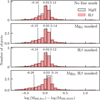 |
Fig. 16 Logarithmic difference between the BH mass estimated from the reconstructed spectra and the original SDSS data. In all cases, the BH mass estimates are consistent and do not appear to depend on the emission line used. |
5.4 Reconstruction of the Lyman-α forest and the Lyman-α emission line
Finally, we tested how well the model reconstructs the Lyman-α forest and the blue side of the Lyman-α emission line. We stress that, contrary to the other methods we compare against in this section, QUEST was not optimised for this task. However, as shown in the following, the model already performs competitively. We choose the GP model because it fully covers the required rest-frame wavelength range.
The key idea is to reconstruct the unabsorbed quasar continuum blueward of the Lyman-α emission line (1026–1210 Å) using the unabsorbed quasar continuum redward of it (1260–2000 Å). The reconstruction should be accurate and unbiased: both requirements are crucially important. This enables several scientific cases: it allows one to chronicle the end of reionisation (see e.g. Bosman et al. 2022) and its global timeline (Hennawi et al. 2025; Ďurovčíková et al. 2024), to measure the temperature of the IGM (Etezad-Razavi et al. 2026), or to determine the size of quasar proximity zones, and to constrain quasar lifetimes (Onorato et al. 2026; Rojas-Ruiz et al. 2025).
In order to estimate the performance of a method, one has to choose metrics and a test set. We followed Bosman et al. (2021) and used the same dataset used to train the model, where the "true" unabsorbed continuum is estimated using Dall'Aglio et al. (2008) (Sect. 2.1). We then compared the reconstruction provided by QUEST with the SDSS spectra. The fractional difference with respect to the truth (bias) and 16th–84th percentiles range (scatter) were used as a comparison metric with other methods. We started by selecting all the quasars in the GP datasets that cover 1026–2000 Å. Effectively, this is equivalent to restricting the comparison to the 781 quasars with Z_PIPE ≳2.55. For each of them, we masked out the region outside 1260–2000 Å, fed the spectra to the VAE, reconstructed them, and compared the reconstructions with the unabsorbed continuum. The results are shown in Fig. 17, where we plot the median bias with the solid blue line and the 16th–84th (2.5th–97.5th) percentiles the grey (light grey) shaded regions. The reconstruction provided by QUEST overestimates the true continuum (with the overestimation being between 2% and 5%, and a median of 2.8%). The 1σ scatter is around 10% (+0.109/−0.092), whereas the 2σ scatter is much larger (0.301/−0.194) and strongly asymmetric (that is, the model tends to overestimate the unabsorbed continuum). Compared to the results presented in Bosman et al. (2021), QUEST performs similarly to Neighbours, outperforming Power-Law and PCA-Pâris-10 but being outperformed by PCANN-QSANNdRA and PCA-Davies-nominal.
6 Discussion
Machine-learning models are becoming increasingly common in extragalactic astronomy and in the study and search for quasars and AGNs. Among others, ML models have been deployed to select quasars from large photometric catalogues (e.g. Byrne et al. 2024; Fu et al. 2025), classify optical spectra and estimate their redshift (e.g. Busca & Balland 2018; Moradi et al. 2024), identify outliers and peculiar sources (Tiwari & Vivek 2025), reconstruct the unabsorbed continuum leftward of the Lyman-α emission line (Pistis et al. 2025; Hahn et al. 2025), or directly estimate the quasar's black hole mass (He et al. 2022; Eilers et al. 2022). Although many of the models mentioned above are tailored to specific tasks, the one presented here can address multiple problems effectively. Nevertheless, it is instructive to compare the spectra it generates with those produced by previous works and to point out the limitations that we are aware of: these will be addressed in future works.
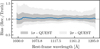 |
Fig. 17 Bias as a function of the rest-frame wavelength in reconstructing the unabsorbed quasar continuum. |
6.1 Comparison with available quasar models
We considered the models published in Temple et al. (2021, qsogen) and McGreer et al. (2021, SimQSO) and qualitatively compared their median sampled spectra with our own. We show in the left two panels of Fig. 18 our median sampled spectrum in black, the 16th–84th percentile range with a grey shaded band, and three different realisations of quasar spectra from qsogen, at three different redshifts: z = 0,1.5,3.0. The choice of redshifts for the QSOGen spectra is somewhat arbitrary but includes a regime where the contribution of the host galaxy is expected to be significant (z = 0, purple), one that is comparable to the mean redshift of our training data (z = 1.5, green), and one that is slightly above the maximum redshift encompassed by our training set (z = 3.0, red). We do not change any parameter from the default ones, with the exception of turning off the absorption of the IGM. This also enables us to compare our reconstruction of the Lyman forest with a completely independent approach. In general, there is a very good agreement between the qsogen models and our own median spectra, especially at z = 1.5, 3.0. At these redshifts, the most striking difference is a slightly steeper continuum slope, especially evident at longer wavelengths, and somewhat broader rest-frame UV emission lines. The latter is likely a consequence of the averaging over several thousands of realisations to produce the median spectrum, combined with the averaging across the training set performed by the model itself. In addition, it is interesting to note that bluewards of the Lyman-α emission line the spectra generated using qsogen are relatively flat, whereas the median spectrum of our model displays several features. We regard them as real, indicative of the variety of emission features that contribute to the unabsorbed quasar continuum (see e.g. Bosman et al. 2021, for a list of the most relevant emission lines in this wavelength range). The difference can be attributed to the approach adopted in Temple et al. (2021), where the continuum between 970 Å and 1050 Å is simply extrapolated from its value at 1050Å in order to reproduce the observed photometric trends, rather than to faithfully trace the average quasar's spectral properties. Additionally, the Temple et al. (2021) spectrum features a much narrower Lyman-β+O VI complex, with the O VI emission line almost absent; in contrast, our median spectrum appears to capture this feature better, showing a broader line that peaks at an intermediate wavelength between the two emission lines. This correctly reflects theoretical expectations, where the Lyman-β emission line preferentially decays to Lyman-α by emitting an Hα photon instead of directly decaying to the ground state.
On the other hand, the qsogen model generated at z = 0 exhibits significant differences with respect to the median sampled spectrum. The emission lines are stronger, and the spectrum appears redder: both effects can be explained by considering the selection effect in the SDSS catalogue, on which the Temple et al. (2021) calibrates their model. Indeed, low-z quasars have, on average, lower intrinsic luminosity than their higher redshift counterparts. Due to the Baldwin effect, this leads to stronger emission lines. In addition, the contribution of the host galaxy becomes more significant, enhancing the flux at longer wavelengths, and producing redder spectra.
Comparing against SimQSO (Fig. 18, right panels) is not straightforward, as SimQSO allow significant customisation to all spectral components. For the purpose of this comparison, we employ the same parameters as previously used in Schindler et al. (2023). Overall, we find very good agreement between the two models, with the most notable exception being the Lyman-α emission line, which appears to be stronger in our sampled composite. However, it is worth emphasising that the model we presented here is completely data-driven and did not require any tweaking: through training, the Info-VAE learnt to appropriately reproduce quasar spectra features without the need to introduce ad hoc, tunable parameters.
6.2 Limitation of the model
Despite its flexibility and capabilities, the model has some limitations that we aim to address in the future.
Limited training set: the training set we used to train the model is, by design, limited to typical, bright SDSS type-I quasars. Since the publication of the SDSS DR16Q catalogue, major quasar catalogues have been released, including DESI DR1 (DESI Collaboration 2025) and the nineteenth SDSS data release itself. DESI spectra could prove especially useful in improving the training set, as they would allow the inclusion of fainter targets and thus the sampling of a larger parameter space. Additionally, value-added catalogues, such as Wu & Shen (2022), would allow improved quasar redshifts compared to Z_PIPE. We plan to address these points in the next iteration of QUEST. Finally, one could produce dedicated training sets to generate large samples of quasar spectra of under-represented populations.
Wavelength coverage: a second, significant, limitation of the model is the limited wavelength coverage of the spectra we train the VAE on. This implies that spectra in the highest-redshift bins will contribute mainly to the bluest portion of the wavelength grid, whereas the spectra at low redshift will contribute to the reddest wavelengths. Because of this, we are sceptical that the model fully captures the physical correlations between the rest-frame UV and optical properties. In this context, including NIR from Euclid (covering the wavelength range 1.21–1.89 μm, albeit with low spectral resolution of R ~ 450, Euclid Collaboration 2023) could lead to significant improvements.
Model architecture and input format: recent advances in ML could be incorporated in the model architecture. Several works have attempted to introduce convolutional and attention layers in AEs and VAEs, obtaining good performance and interpretable results (see e.g. Melchior et al. 2023): testing the effect of these layers in our model could be helpful in unlocking additional performance. Moreover, by design, our model incorporates a coverage mask, concatenated to each spectrum, as input. Although this is needed to inform the model about the wavelength coverage of each spectrum, it might have unwanted side effects, such as introducing or reinforcing redshift trends. An approach like that presented in Hahn et al. (2025) could mitigate this problem.
Conditional VAE: to aid with the search of a particular type of quasar, or to understand whether quasars with particular spectral properties are systematically missed by a survey ora selection algorithm, one could condition the VAE on a given quasar property, such as the luminosity, the BH mass, or the quasar's redshift. This would allow for targeted generation of quasar spectra and offers insight into the properties of a particular population. In addition, conditioning the VAE on redshift and luminosity might mitigate biases inherited from the training dataset selection function and allow the model to learn the relevant quasar physics more easily. We plan to further develop these ideas and implement them in QUEST.
Estimate quasar properties directly from the latent space, as a complementary approach to inferring them to reconstructed spectra. This requires the model to have learnt the relevant physics and probably dedicated training datasets. The GP model, for example, does not have access to a fully connected parameter space: this is evident from Fig. 3, where the high-z-faint and the low-z–bright regimes are not fully populated.
7 Conclusion
We presented a general model for quasar spectra based on an information maximising variational auto-encoder architecture. The model is capable of generating realistic quasar spectra that can be post-processed for different purposes that range from generating synthetic photometry to imputing BAL features and to reconstructing the emission line to then estimating the quasar black hole mass. We list our particular results below:
We produced three complementary datasets: the general purpose, the full overlap blue, and full overlap red datasets. In all cases, we started from the SDSS DR16Q quasar catalogue, and we applied quality cuts to select type-I quasars without absorption systems or intrinsic reddening. The GP dataset was designed to cover the largest wavelength interval, from 980 Å to 5500 Å with the goal of producing a versatile model. The full overlap blue and red datasets, instead, were designed to show the adaptability of the model and are geared towards more specific science cases, namely imputing BAL features and reconstructing emission lines with the purpose of estimating the corresponding quasar black hole mass;
After training the model and verifying that it provided an accurate reconstruction of the SDSS spectra, we investigated whether the latent space correlates with physical properties. To do this, we first developed an intuition for which spectral features were affected by each latent dimension by varying a single latent space dimension, reconstructing the spectra, and inspecting the results. We then reduced the dimension of the VAE latent space using UMAP and searched for a correlation with the quasar properties in the resulting embedding. Finally, we applied GMM-MI, an estimator for mutual information, to robustly quantify the correlation between latent space dimensions and quasar properties. Through these tests, we identified the correlation between latent dimensions and the quasar continuum slope, the continuum luminosity, the absolute i-band magnitude, the black hole mass, the emission line equivalent width, and the line luminosity. Although it is possible that the model picked up physical quasar physical properties, we cannot exclude the fact that at least part of these correlations stem from the selection function inherited from our training dataset (i.e. a combination of the SDSS selection function, the requirement of SN_MEDIAN_ALL > 15, and the cleaning procedure we applied). The strong correlation between redshift and UMAP representation (Fig. 10) might be a hint in this direction; – To show their capabilities, we employed the model trained on the GP dataset to generate synthetic quasar photometry, the model trained on the FOB dataset to input BAL features, and the model trained on the FOR dataset to reconstruct emission lines in order to estimate the black hole masses. We found that the photometry estimated from the quasar spectra faithfully reproduced the SDSS colours of the low-z quasar and the colours of the quasars with z > 5.3 from Fan et al. (2023). The FOB model, while providing a satisfactory reconstruction in most cases, struggled to accurately reconstruct asymmetric and blueshifted emission lines (e.g. the C IV). The BH masses obtained from fitting FOR spectra agree well in general with the BH masses we estimated from the real SDSS quasar spectra (although they are overestimated by a factor of ~1.25), with the most significant differences arising for objects with the highest BH masses. A detailed investigation of these problems is beyond the scope of this paper, but the lack of training data might hamper the capabilities of the model. In the future, we aim to further perfect the model by expanding the training dataset to include more data, generate targeted datasets (e.g. that include quasars with broad absorption lines, weak emission lines, or that are reddened) and improve the current architecture to include recent advances in ML. This will allow us, for example, to efficiently select these sources from current and future astronomical surveys.
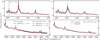 |
Fig. 18 Median spectrum, computed from 50 000 realisations sampled from our model and synthetic spectra from Temple et al. (2021, left panels) or McGreer et al. (2021, right panels). In all plots, the solid black line represents the median spectrum from this work with the corresponding 16th-84th percentile range. In the two left panels, the coloured lines represent realisations of the default qsogen model at different redshifts, whereas in the right panels we show the median SimQSO spectrum with tweaked emission line strength (from Schindler et al. 2023) in red. |
Data availability
Full Tables A.1 and E.1 are available at the CDS via https://cdsarc.cds.unistra.fr/viz-bin/cat/J/A+A/709/A241. Our QUEST tool is available here: https://github.com/cosmic-dawn-group/QUEST
Acknowledgements
The code underlying this work makes significant use of the following open-source projects: numpy (Harris et al. 2020), astropy (Robitaille et al. 2013; Astropy Collaboration 2018, 2022), matplotlib (Hunter 2007), pandas (pandas development team 2025) and numba (Lam et al. 2015). The extinction curves are computed via a custom Python package (https://github.com/G-Francio/numba_extinction) following Gordon (2024). This work has been supported by the Deutsche Forschungsgemeinschaft (German Research Foundation; Project Nos. 518006966 to J.-T.S. and F.G., and 506672582 to S.E.I.B.). LLS acknowledges support by the Deutsche Forschungsgemeinschaft (DFG, German Research Foundation) under Germany's Excellence Strategy – EXC 2121 "Quantum Universe" – 390833306. J.F.H. acknowledges support from the European Research Council (ERC) under the European Union's Horizon 2020 research and innovation programme (grant agreement No. 885301), from the National Science Foundation (NSF) under Grant No. 2307180, and from NASA under the Astrophysics Data Analysis Programme (ADAP, Grant No. 80NSSC21K1568). RAM acknowledges support from the Swiss National Science Foundation (SNSF) through project grant 200020_207349. Funding for the Sloan Digital Sky Survey IV has been provided by the Alfred P. Sloan Foundation, the U.S. Department of Energy Office of Science, and the Participating Institutions. SDSS-IV acknowledges support and resources from the Center for High Performance Computing at the University of Utah. The SDSS website is www.sdss4.org. SDSS-IV is managed by the Astrophysical Research Consortium for the Participating Institutions of the SDSS Collaboration including the Brazilian Participation Group, the Carnegie Institution for Science, Carnegie Mellon University, Center for Astrophysics I Harvard & Smithsonian, the Chilean Participation Group, the French Participation Group, Instituto de Astrofísica de Canarias, The Johns Hopkins University, Kavli Institute for the Physics and Mathematics of the Universe (IPMU) / University of Tokyo, the Korean Participation Group, Lawrence Berkeley National Laboratory, Leibniz Institut für Astrophysik Potsdam (AIP), Max-Planck-Institut für Astronomie (MPIA Heidelberg), Max-Planck-Institut für Astrophysik (MPA Garching), Max-Planck-Institut für Extraterrestrische Physik (MPE), National Astronomical Observatories of China, New Mexico State University, New York University, University of Notre Dame, Observatário Nacional/MCTI, The Ohio State University, Pennsylvania State University, Shanghai Astronomical Observatory, United Kingdom Participation Group, Universidad Nacional Autónoma de México, University of Arizona, University of Colorado Boulder, University of Oxford, University of Portsmouth, University of Utah, University of Virginia, University of Washington, University of Wisconsin, Vanderbilt University, and Yale University.
References
- Alsing, J., Peiris, H., Leja, J., et al. 2020, ApJS, 249, 5 [CrossRef] [Google Scholar]
- Ansel, J., Yang, E., He, H., et al. 2024, in ASPLOS ’24, 2, Proceedings of the 29th ACM International Conference on Architectural Support for Programming Languages and Operating Systems, Volume 2 (New York, NY, USA: Association for Computing Machinery), 929 [Google Scholar]
- Astropy Collaboration (Price-Whelan, A. M., et al.) 2018, AJ, 156, 123 [Google Scholar]
- Astropy Collaboration (Price-Whelan, A. M., et al.) 2022, ApJ, 935, 167 [NASA ADS] [CrossRef] [Google Scholar]
- Baldwin, J. A. 1977, ApJ, 214, 679 [NASA ADS] [CrossRef] [Google Scholar]
- Barnett, R., Warren, S. J., Cross, N. J. G., et al. 2021, MNRAS, 501, 1663 [Google Scholar]
- Bañados, E., Venemans, B. P., Mazzucchelli, C., et al. 2018, Nature, 553, 473 [Google Scholar]
- Bañados, E., Schindler, J.-T., Venemans, B. P., et al. 2023, ApJS, 265, 29 [CrossRef] [Google Scholar]
- Belladitta, S., Bañados, E., Xie, Z.-L., et al. 2025, A&A, 699, A335 [NASA ADS] [CrossRef] [EDP Sciences] [Google Scholar]
- Boroson, T. A., & Green, R. F. 1992, ApJS, 80, 109 [Google Scholar]
- Bosman, S. E. I., Davies, F. B., Becker, G. D., et al. 2022, MNRAS, 514, 55 [NASA ADS] [CrossRef] [Google Scholar]
- Bosman, S. E. I., Ďurovčíková, D., Davies, F. B., & Eilers, A. C. 2021, MNRAS, 503, 2077 [CrossRef] [Google Scholar]
- Busca, N., & Balland, C. 2018, QuasarNET: Human-level spectral classification and redshifting with Deep Neural Networks, MMRAS, submitted [Google Scholar]
- Byrne, X., Meyer, R. A., Farina, E. P., et al. 2024, MNRAS, 530, 870, [Google Scholar]
- Carswell, R. F., Whelan, J. A. J., Smith, M. G., Boksenberg, A., & Tytler, D. 1982, MNRAS, 198, 91 [NASA ADS] [Google Scholar]
- Chambers, K. C., Magnier, E. A., Metcalfe, N., et al. 2016, The Pan-STARRS1 Surveys [Google Scholar]
- Champagne, J. B., Casey, C. M., Finkelstein, S. L., et al. 2023, ApJ, 952, 99 [NASA ADS] [CrossRef] [Google Scholar]
- Chiang, Y.-K. 2023, ApJ, 958, 118 [NASA ADS] [CrossRef] [Google Scholar]
- Choi, H., Leighly, K. M., Terndrup, D. M., et al. 2022, ApJ, 937, 74 [NASA ADS] [CrossRef] [Google Scholar]
- Dall’Aglio, A., Wisotzki, L., & Worseck, G. 2008, A&A, 491, 465 [Google Scholar]
- Decleir, M., Gordon, K. D., Andrews, J. E., et al. 2022, ApJ, 930, 15 [NASA ADS] [CrossRef] [Google Scholar]
- Ďurovčíková, D., Eilers, A.-C., Chen, H., et al. 2024, ApJ, 969, 162 [Google Scholar]
- DESI Collaboration (Abdul-Karim, M., et al.) 2025, Data Release 1 of the Dark Energy Spectroscopic Instrument [Google Scholar]
- Edge, A., Sutherland, W., Kuijken, K., et al. 2013, The Messenger, 154, 32 [NASA ADS] [Google Scholar]
- Eilers, A.-C., Hogg, D. W., Schölkopf, B., et al. 2022, ApJ, 938, 17 [Google Scholar]
- Etezad-Razavi, S., Bosman, S. E. I., & Davies, F. B. 2026, ApJ, 998, 179 [Google Scholar]
- Euclid Collaboration (Gabarra, L., et al.) 2023, A&A, 676, A34 [NASA ADS] [CrossRef] [EDP Sciences] [Google Scholar]
- Euclid Collaboration (Mellier, Y., et al.) 2025, A&A, 697, A1 [Google Scholar]
- Fan, X., Strauss, M. A., Becker, R. H., et al. 2006, AJ, 132, 117 [NASA ADS] [CrossRef] [Google Scholar]
- Fan, X., Bañados, E., & Simcoe, R. A. 2023, ARA&A, 61, 373 [NASA ADS] [CrossRef] [Google Scholar]
- Farina, E. P., Schindler, J.-T., Walter, F., et al. 2022, ApJ, 941, 106 [NASA ADS] [CrossRef] [Google Scholar]
- Fitzpatrick, E. L., & Massa, D. 1999, ApJ, 525, 1011 [Google Scholar]
- Fitzpatrick, E. L., Massa, D., Gordon, K. D., Bohlin, R., & Clayton, G. C. 2019, ApJ, 886, 108 [Google Scholar]
- Fu, Y., Wu, X.-B., Bouwens, R. J., et al. 2025, ApJS, 279, 54 [Google Scholar]
- Gordon, K. D. 2024, J. Open Source Softw., 9, 7023 [NASA ADS] [CrossRef] [Google Scholar]
- Gordon, K. D., Cartledge, S., & Clayton, G. C. 2009, ApJ, 705, 1320 [NASA ADS] [CrossRef] [Google Scholar]
- Gordon, K. D., Misselt, K. A., Bouwman, J., et al. 2021, ApJ, 916, 33 [NASA ADS] [CrossRef] [Google Scholar]
- Gordon, K. D., Clayton, G. C., Decleir, M., et al. 2023, ApJ, 950, 86 [CrossRef] [Google Scholar]
- Gretton, A., Borgwardt, K. M., Rasch, M. J., Schölkopf, B., & Smola, A. 2012, J. Mach. Learn. Res., 13, 723 [Google Scholar]
- Guo, H., Shen, Y., & Wang, S. 2018, Astrophysics Source Code Library [record ascl:1809.008] [Google Scholar]
- Hahn, C., Gontcho, S. G. A., Melchior, P., et al. 2025, Reconstructing Quasar Spectra and Measuring the Lyα Forest with SpenderQ [Google Scholar]
- Harris, C. R., Millman, K. J., van der Walt, S. J., et al. 2020, Nature, 585, 357 [NASA ADS] [CrossRef] [Google Scholar]
- He, Y., Guo, Q., & Shao, S. 2022, Res. Astron. Astrophys., 22, 085014 [Google Scholar]
- Hennawi, J. F., Kist, T., Davies, F. B., & Tamanas, J. 2025, MNRAS, 539, 2621 [Google Scholar]
- Higgins, I., Matthey, L., Pal, A., et al. 2017, in International Conference on Learning Representations [Google Scholar]
- Hunter, J. D. 2007, Comput. Sci. Eng., 9, 90 [NASA ADS] [CrossRef] [Google Scholar]
- Inayoshi, K., Visbal, E., & Haiman, Z. 2020, ARA&A, 58, 27 [NASA ADS] [CrossRef] [Google Scholar]
- Kang, Y., Hennawi, J. F., Schindler, J.-T., Tamanas, J., & Nanni, R. 2025, MNRAS, 541, 2815 [Google Scholar]
- Kingma, D. P., & Ba, J. 2017, Adam: A Method for Stochastic Optimization [arXiv:1412.6988] [cs] [Google Scholar]
- Kingma, D. P., & Welling, M. 2013, Auto-Encoding Variational Bayes [Google Scholar]
- Kirkby, D., Robitaille, T., Weaver, B. A., et al. 2024, desihub/speclite: Bug fix release: General clean-up prior to refactoring package infrastructure [Google Scholar]
- Kist, T., Hennawi, J. F., & Davies, F. B. 2025, MNRAS, 538, 2704 [Google Scholar]
- Kormendy, J., & Ho, L. C. 2013, ARA&A, 51, 511 [Google Scholar]
- Kullback, S., & Leibler, R. A. 1951, Ann. Math. Statist., 22, 79 [Google Scholar]
- Lam, S. K., Pitrou, A., & Seibert, S. 2015, in Proceedings of the Second Workshop on the LLVM Compiler Infrastructure in HPC, LLVM '15 (New York, NY, USA: Association for Computing Machinery), 1 [Google Scholar]
- Lawrence, A., Warren, S. J., Almaini, O., et al. 2007, MNRAS, 379, 1599 [Google Scholar]
- Li, J., Silverman, J. D., Izumi, T., et al. 2022, ApJ, 931, L11 [NASA ADS] [CrossRef] [Google Scholar]
- Lucie-Smith, L., Despali, G., & Springel, V. 2024, MNRAS, 532, 164 [Google Scholar]
- Lucie-Smith, L., Peiris, H. V., & Pontzen, A. 2024, Phys. Rev. Lett., 132, 031001 [Google Scholar]
- Lusso, E., Worseck, G., Hennawi, J. F., et al. 2015, MNRAS, 449, 4204 [Google Scholar]
- Lyke, B. W., Higley, A. N., McLane, J. N., et al. 2020, ApJS, 250, 8 [NASA ADS] [CrossRef] [Google Scholar]
- Maas, A. L. 2013, in ICML'13: Proceedings of the 30th International Conference on International Conference on Machine Learning, 28 [Google Scholar]
- Matsuoka, Y., Iwasawa, K., Onoue, M., et al. 2025, ApJS, 280, 68 [Google Scholar]
- Matthews, B. M., Dix, C., Shemmer, O., et al. 2023, ApJ, 950, 95 [NASA ADS] [CrossRef] [Google Scholar]
- Matthews, B. M., Shemmer, O., Dix, C., et al. 2021, ApJS, 252, 15 [NASA ADS] [CrossRef] [Google Scholar]
- McGreer, I., Moustakas, J., & Schindler, J. 2021, Astrophysics Source Code Library [record ascl:2186.888] [Google Scholar]
- McInnes, L., Healy, J., & Astels, S. 2017, J. Open Source Softw., 2, 205 [NASA ADS] [CrossRef] [Google Scholar]
- McInnes, L., Healy, J., & Melville, J. 2018, arXiv e-prints [arXiv: 1882.83426] [Google Scholar]
- McMahon, R. G., Banerji, M., Gonzalez, E., et al. 2013, The Messenger, 154, 35 [NASA ADS] [Google Scholar]
- Melchior, P., Liang, Y., Hahn, C., & Goulding, A. 2023, AJ, 166, 74 [NASA ADS] [CrossRef] [Google Scholar]
- Meyer, R. A., Decarli, R., Walter, F., et al. 2022, ApJ, 927, 141 [NASA ADS] [CrossRef] [Google Scholar]
- Moradi, R., Rastegarnia, F., Wang, Y., & Mirtorabi, M. T. 2024, MNRAS, 533, 1976 [NASA ADS] [CrossRef] [Google Scholar]
- Mortlock, D. J., Warren, S. J., Venemans, B. P., et al. 2011, Nature, 474, 616 [Google Scholar]
- Nanni, R., Hennawi, J. F., Wang, F., et al. 2022, MNRAS, 515, 3224 [NASA ADS] [CrossRef] [Google Scholar]
- Neeleman, M., Novak, M., Venemans, B. P., et al. 2021, ApJ, 911, 141 [NASA ADS] [CrossRef] [Google Scholar]
- Oke, J. B., & Gunn, J. E. 1983, ApJ, 266, 713 [NASA ADS] [CrossRef] [Google Scholar]
- Onorato, S., Hennawi, J. F., Pizzati, E., Venemans, B. P., & Eilers, A.-C. 2026, MNRAS, 547, stag388 [Google Scholar]
- pandas development team, T. 2025, pandas-dev/pandas: Pandas [Google Scholar]
- Piras, D., Peiris, H. V., Pontzen, A., et al. 2023, Mach. Learn. Sci. Technol., 4, 025006 [Google Scholar]
- Pistis, F., Fumagalli, M., Fossati, M., et al. 2025, A&A, 698, A292 [NASA ADS] [CrossRef] [EDP Sciences] [Google Scholar]
- Planck Collaboration VI. 2020, A&A, 641, A6 [NASA ADS] [CrossRef] [EDP Sciences] [Google Scholar]
- Pâris, I., Petitjean, P., Ross, N. P., et al. 2017, A&A, 597, A79 [NASA ADS] [CrossRef] [EDP Sciences] [Google Scholar]
- Qin, Y., Mesinger, A., Prelogovic, D., et al. 2025, PASA, 42, e049 [Google Scholar]
- Rankine, A. L., Hewett, P. C., Banerji, M., & Richards, G. T. 2020, MNRAS, 492, 4553 [CrossRef] [Google Scholar]
- Robitaille, T. P., Tollerud, E. J., Greenfield, P., et al. 2013, A&A, 558, A33 [NASA ADS] [CrossRef] [EDP Sciences] [Google Scholar]
- Rojas-Ruiz, S., Momjian, E., Davies, F. B., et al. 2025, ApJ, 985, 34 [Google Scholar]
- Rumelhart, D. E., & McClelland, J. L. 1987, in Parallel Distributed Processing: Explorations in the Microstructure of Cognition: Foundations (MIT Press), 318 [Google Scholar]
- Salvestrini, F., Feruglio, C., Tripodi, R., et al. 2025, A&A, 695, A23 [NASA ADS] [CrossRef] [EDP Sciences] [Google Scholar]
- Salviander, S., Shields, G. A., Gebhardt, K., & Bonning, E. W. 2007, ApJ, 662, 131 [NASA ADS] [CrossRef] [Google Scholar]
- Schindler, J.-T., Farina, E. P., Banados, E., et al. 2020, ApJ, 905, 51 [CrossRef] [Google Scholar]
- Schindler, J.-T., Bañados, E., Connor, T., et al. 2023, ApJ, 943, 67 [NASA ADS] [CrossRef] [Google Scholar]
- Selsing, J., Fynbo, J. P. U., Christensen, L., & Krogager, J.-K. 2016, A&A, 585, A87 [NASA ADS] [CrossRef] [EDP Sciences] [Google Scholar]
- Shannon, C. E. 1948, Bell Syst. Tech. J., 27, 379 [Google Scholar]
- Shen, Y., Hall, P. B., Horne, K., et al. 2019, ApJS, 241, 34 [NASA ADS] [CrossRef] [Google Scholar]
- Silverman, J. D., Li, J., Ding, X., et al. 2025, ApJ, 995, L67 [Google Scholar]
- Spilker, J. S., Champagne, J. B., Fan, X., et al. 2025, ApJ, 982, 72 [Google Scholar]
- Temple, M. J., Hewett, P. C., & Banerji, M. 2021, MNRAS, 508, 737 [NASA ADS] [CrossRef] [Google Scholar]
- Tiwari, A., & Vivek, M. 2025, A&A, 699, A132 [NASA ADS] [CrossRef] [EDP Sciences] [Google Scholar]
- Tsuzuki, Y., Kawara, K., Yoshii, Y., et al. 2006, ApJ, 650, 57 [NASA ADS] [CrossRef] [Google Scholar]
- Umeda, H., Ouchi, M., Kageura, Y., et al. 2026, ApJ, 997, 86 [Google Scholar]
- Vanden Berk, D. E., Richards, G. T., Bauer, A., et al. 2001, AJ, 122, 549 [Google Scholar]
- Vestergaard, M., & Wilkes, B. J. 2001, ApJS, 134, 1 [Google Scholar]
- Volonteri, M., Habouzit, M., & Colpi, M. 2021, Nat. Rev. Phys., 3, 732 [NASA ADS] [CrossRef] [Google Scholar]
- Wang, F., Davies, F. B., Yang, J., et al. 2020, ApJ, 896, 23 [NASA ADS] [CrossRef] [Google Scholar]
- Wang, F., Yang, J., Fan, X., et al. 2021, ApJ, 907, L1 [Google Scholar]
- Wang, F., Yang, J., Hennawi, J. F., et al. 2023, ApJ, 951, L4 [NASA ADS] [CrossRef] [Google Scholar]
- Wenzl, L., Schindler, J.-T., Fan, X., et al. 2021, AJ, 162, 72 [NASA ADS] [CrossRef] [Google Scholar]
- Whittet, D. C. B., & van Breda, I. G. 1980, MNRAS, 192, 467 [NASA ADS] [CrossRef] [Google Scholar]
- Wu, Q., & Shen, Y. 2022, ApJS, 263, 42 [NASA ADS] [CrossRef] [Google Scholar]
- Yang, J., Wang, F., Fan, X., et al. 2020, ApJ, 897, L14 [Google Scholar]
- Yang, J., Wang, F., Fan, X., et al. 2021, ApJ, 923, 262 [NASA ADS] [CrossRef] [Google Scholar]
- Yang, D.-M., Schindler, J.-T., Nanni, R., et al. 2024, MNRAS, 528, 2679 [CrossRef] [Google Scholar]
- Young, P. J., Sargent, W. L. W., Boksenberg, A., Carswell, R. F., & Whelan, J. A. J. 1979, ApJ, 229, 891 [Google Scholar]
- Zhao, S., Song, J., & Ermon, S. 2017, InfoVAE: Information Maximizing Variational Autoencoders [Google Scholar]
Appendix A Median composite of the General Purpose training dataset
Here and in electronic form at CDS, we provide the data underlying Fig. 4. The columns "Rest-Frame wavelength" and "# of spectra" contain, respectively, the rest-frame wavelength array we use to sample each spectra and the number of spectrum contributing to the composite. The column "Flux density" contains the median flux density, per pixel, of the GP sample. Percentiles columns contain the nth flux percentile, as shown in Fig. 4. The units of the median flux (and of each percentile column) are arbitrary, as all spectra are normalised between 2350 Å and 2360 Å.
Appendix B Sampled median compared to median for FOR and FOB models
In Fig. B.1 we present the comparison between the median of sampled spectra and the median of the input data for the FOR and FOB datasets. As was the case for the GP dataset, the input spectra are normalised in a window between 2350 Å and 2360 Å.
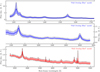 |
Fig. B.1 Sampled spectra from the FOR and FOB models compared to the input spectra. In all panels, the black solid and dashed lines indicate the median, 16th and 84th percentile of the input data. The solid grey line represents the median spectrum of 10 000 realisations sampled from the VAE, while the shaded area encompasses the 16th and 84th percentile of the same sampled data. |
Appendix C Latent space distributions
In Fig. C.1 we present a corner plot showing each latent space dimension for the GP model. Almost all the latents are approximately Gaussian, with the exception of LD5, featuring an asymmetric distribution (corresponding to the secondary peak highlighted in red) and to a lesser extent LD7, featuring an extended "tail", highlighted in blue. We visualise the spectra corresponding to these features by plotting the median spectrum, and find them to correspond to low-z, reddened spectra and spectra that have absorption in the Lyman-a emission line, respectively.
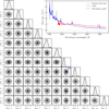 |
Fig. C.1 Corner plot showing the latent space dimensions for the GP model. We highlight in red the "secondary peak" in LD1–LD5 and in blue the extended tail in LD7. In the top right we show the median SDSS spectra populating the "tail" (blue) and the secondary peak (red). These appear to be quasar with either a weak or absorbed Lyman-a emission line, and reddened spectra that were not excluded by our preprocessing. |
Appendix D Latent space variations
We present in Fig. D.1 the latent space variations for all the eleven dimension of the GP model. As for Fig. 8, we compute the variations by decoding mock latent space vectors where only one dimension is varied. The varied dimension is marked in the upper right corner.
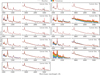 |
Fig. D.1 Latent space variations for the eleven dimensions of the GP model. |
Appendix E List of SDSS identifiers in each HDBScan cluster
SDSS identifier in each cluster. The full table will be made available at the CDS.
Appendix F BAL quasars
We present in Fig. F.1 the remaining six spectra of BAL quasars with the reconstruction from the model. In most cases, the model struggles to model the unabsorbed continuum and the emission lines, leading to sub-par reconstructions.
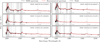 |
Fig. F.1 Spectra of the six remaining quasars used to test the imputation capabilities of the model. As in Fig. F.1, we show in black the input spectrum, in red the reconstruction, and with the shaded, grey areas the masked regions. The SDSS identifier is indicated in the top right corner. |
We indicate in typeface font the column names of the SDSS DR16Q catalogue.
Defined, according to the SDSS documentation, as "Median S/N value of all good spectroscopic pixels."
The SDSS DR16Q provides the absolute i-band magnitude, which we used in place of the M1450.
Retrieved from https://data.sdss.org/sas/dr12/boss/qso/DR12Q/DR12Q_BAL.fits
All Tables
SDSS identifier in each cluster. The full table will be made available at the CDS.
All Figures
|
Fig. 1 Top panel: example of SDSS spectra at different redshifts included in the GP dataset. Bottom panel: example of a spectrum from the GNIRS-DQS survey, highlighting the extended coverage at redder wavelengths. The spectral gaps are are due to telluric absorptions. |
| In the text | |
|
Fig. 2 Examples of rejected spectra, and the cause of rejection. The black line shows the original SDSS spectrum, the red line shows the nominal uncertainty, and the light grey line shows the zero-flux level. |
| In the text | |
|
Fig. 3 Density plot showing the redshift-absolute i-band magnitude distribution for the spectra that meet the selection criteria. The colour map shows the number of spectra in each contour line. |
| In the text | |
|
Fig. 4 Median spectrum and logarithmic number of spectra contributing to the median in each pixel. Top panel: Median spectrum of the quasars included in the training set (thick solid black line) compared to the Vanden Berk et al. (2001) (thin solid red line). The shaded regions represent the 16th–84th percentiles (dark grey) and the 1st–99th percentile (light grey). The vertical blue band represents the region in which we computed the normalisation factor for each spectrum. Middle panel: Same as the top panel, but for the Selsing et al. (2016) composite spectrum. Bottom panel: Logarithmic number of spectra contributing to each pixel in the median spectrum. By construction, all spectra contribute to the region between 2300–2600 Å. |
| In the text | |
|
Fig. 5 Schematic representation of the model architecture, input, and output. The network receives as input the concatenation of an SDSS spectrum, normalised by the median spectrum, and the coverage mask (top left panel). It then encodes the input to produce a latent space representation Z, that is decoded to produce a new spectrum (top right panel). The new spectrum (shown in red) covers a wider wavelength range compared to the corresponding input (shown in black) and is generally less noisy. The encoder and decoder are built as the reverse of each other by combining several hidden layers, denoted in the schematic by HL followed by the corresponding output dimension. Each hidden layer is a combination of a linear layer, followed by a BatchNormlD layer, and the activation function (bottom left). |
| In the text | |
|
Fig. 6 Sampled spectra from the GP model compared to the input spectra. In both panels, the solid and dashed black lines indicate the median, 16th, and 84th percentile of the input data respectively. The solid grey line represents the median spectrum of 10 000 realisations sampled from the VAE, while the shaded area encompasses the 16th and 84th percentile of the same sampled data. The model is able to accurately reproduce the median and the variance of the input spectra. We note that all spectra are normalised using the flux between 2350 Å and 2360 Å as reference. The comparison between median sampled spectrum and median input for the FOR and FOB models is shown in Fig. B.1. |
| In the text | |
|
Fig. 7 Training and validation losses for the GP network as a function of the number of latent dimension. |
| In the text | |
|
Fig. 8 Decoded spectra obtained from a mock latent space, where we varied a single latent dimension (indicated in the top right corner) while keeping the others constant. In order to better visualise the results we use a different scale for the blue and red side of the decoded spectra; the two, however, smoothly join. We show in this figure the five latent space dimensions that produce the largest variations and in Fig. D.1 all the latent dimensions. |
| In the text | |
|
Fig. 9 Two-dimensional UMAP embedding of the VAE latent space for the GP model. Top panel: Clusters identified in the embedding, highlighted using different colours (orange, green, and red). Outliers (i.e. points that are not associated with any cluster) are shown in purple. For visualisation purposes, the bottom panel shows the median SDSS input spectrum for objects in each cluster, with matching colour-coding. |
| In the text | |
|
Fig. 10 UMAP embedding colour-coded by redshift, absolute i-band magnitude, S/N, galactic extinction, logarithm of the Eddington ratio, and continuum slope (top to bottom, left to right). |
| In the text | |
|
Fig. 11 UMAP representation colour-coded as a function of the bolometric luminosity and the resulting spectra decoded from the latent space point in the direction of evolution. Left panel: UMAP embedding; the points on which we applied the inverse UMAP transformation are highlighted as scatter points and are colour-coded using the average neighbouring colour. Right panel: Spectra decoded from latent space samples highlighted in the left panel and colour-coded according to the respective originating scatter point. |
| In the text | |
|
Fig. 12 Mutual information between all the latent dimensions of the GP model and the ten most correlated variables. |
| In the text | |
|
Fig. 13 SDSS and UKIDSS colours as a function of redshift for the SDSS quasar and our synthetic photometry. The model faithfully reproduces the SDSS median colour at all redshifts, with the exception of the u–g colour, where the absorption from the IGM and the interpolation over the Lyman forest significantly affects the u band. The same happens for UKIDSS colours, albeit with a narrower spread. |
| In the text | |
|
Fig. 14 Same as Fig. 13, but for the high-z sample from (Fan et al. 2023). In this case, we represent the photometry from the real quasars with scatter points instead of presenting the 16th–84th percentile range due to the low number of high redshift quasars. |
| In the text | |
|
Fig. 15 Example of a spectrum with an acceptable reconstruction (top panel), a spectrum for which the model underestimates the Lyman-α and N V complex (middle panel), and a spectrum for which instead the restframe UV and optical emission lines are not well reproduced (bottom panel). We show in black the input spectrum, in red the reconstruction, and with the shaded grey areas the masked out regions. We show the remaining spectra in Fig. F.1. |
| In the text | |
|
Fig. 16 Logarithmic difference between the BH mass estimated from the reconstructed spectra and the original SDSS data. In all cases, the BH mass estimates are consistent and do not appear to depend on the emission line used. |
| In the text | |
|
Fig. 17 Bias as a function of the rest-frame wavelength in reconstructing the unabsorbed quasar continuum. |
| In the text | |
|
Fig. 18 Median spectrum, computed from 50 000 realisations sampled from our model and synthetic spectra from Temple et al. (2021, left panels) or McGreer et al. (2021, right panels). In all plots, the solid black line represents the median spectrum from this work with the corresponding 16th-84th percentile range. In the two left panels, the coloured lines represent realisations of the default qsogen model at different redshifts, whereas in the right panels we show the median SimQSO spectrum with tweaked emission line strength (from Schindler et al. 2023) in red. |
| In the text | |
|
Fig. B.1 Sampled spectra from the FOR and FOB models compared to the input spectra. In all panels, the black solid and dashed lines indicate the median, 16th and 84th percentile of the input data. The solid grey line represents the median spectrum of 10 000 realisations sampled from the VAE, while the shaded area encompasses the 16th and 84th percentile of the same sampled data. |
| In the text | |
|
Fig. C.1 Corner plot showing the latent space dimensions for the GP model. We highlight in red the "secondary peak" in LD1–LD5 and in blue the extended tail in LD7. In the top right we show the median SDSS spectra populating the "tail" (blue) and the secondary peak (red). These appear to be quasar with either a weak or absorbed Lyman-a emission line, and reddened spectra that were not excluded by our preprocessing. |
| In the text | |
|
Fig. D.1 Latent space variations for the eleven dimensions of the GP model. |
| In the text | |
|
Fig. F.1 Spectra of the six remaining quasars used to test the imputation capabilities of the model. As in Fig. F.1, we show in black the input spectrum, in red the reconstruction, and with the shaded, grey areas the masked regions. The SDSS identifier is indicated in the top right corner. |
| In the text | |
Current usage metrics show cumulative count of Article Views (full-text article views including HTML views, PDF and ePub downloads, according to the available data) and Abstracts Views on Vision4Press platform.
Data correspond to usage on the plateform after 2015. The current usage metrics is available 48-96 hours after online publication and is updated daily on week days.
Initial download of the metrics may take a while.