| Issue |
A&A
Volume 709, May 2026
|
|
|---|---|---|
| Article Number | A66 | |
| Number of page(s) | 10 | |
| Section | Planets, planetary systems, and small bodies | |
| DOI | https://doi.org/10.1051/0004-6361/202659075 | |
| Published online | 05 May 2026 | |
Lunar ejecta as the missing piece to resolving lunar cratering asymmetry
1
State Key Laboratory of Lunar and Planetary Sciences, Macau University of Science and Technology,
Macau
999078,
China
2
School of Astronomy and Space Science, Nanjing University,
163 Xianlin Avenue,
Nanjing
210046,
China
3
Key Laboratory of Modern Astronomy and Astrophysics in Ministry of Education, Nanjing University,
China
★ Corresponding author: This email address is being protected from spambots. You need JavaScript enabled to view it.
Received:
22
January
2026
Accepted:
19
March
2026
Abstract
The leading-trailing asymmetry in lunar crater distribution provides a critical record of inner Solar System dynamics, yet the long-standing discrepancy between the observed higher asymmetry and lower theoretical predictions indicates a gap in our understanding of the impactor population. This paper hypothesizes that lunar impact ejecta, which can enter Earth-like orbits and later exit, constitute a component that had previously been unaccounted for. Using numerical simulations, we found that ~25% of escaped ejecta will re-impact the Earth-Moon system within 3 Myr, with about 1.2% striking the Moon. Crucially, these lunar impacts exhibit an extreme leading-trailing asymmetry, with a ratio of 5.9. Our results indicate that the assumption of lunar ejecta, comprising ~15% of total impactors can indeed explain the observed asymmetry, leading to their recognition as active agents shaping the lunar impact record. This work provides new constraints on our understanding of the impact environment of the Earth-Moon system, with direct relevance to the interpretation of lunar geology, the transport of lunar material to Earth, and ongoing space exploration missions.
Key words: methods: miscellaneous / celestial mechanics / meteorites, meteors, meteoroids / Moon
© The Authors 2026
 Open Access article, published by EDP Sciences, under the terms of the Creative Commons Attribution License (https://creativecommons.org/licenses/by/4.0), which permits unrestricted use, distribution, and reproduction in any medium, provided the original work is properly cited.
This article is published in open access under the Subscribe to Open model. This email address is being protected from spambots. You need JavaScript enabled to view it. to support open access publication.
1 Introduction
The lunar surface, largely untouched by geological recycling processes, serves as a pristine archive of the inner Solar System’s impact history. The distribution of craters across this surface is not random; it encodes fundamental information about the dynamics and populations of small bodies that have interacted with the Earth-Moon system over billions of years (Halliday 1964; Wood 1973; Halliday & Griffin 1982; Pinet 1985; Werner & Medvedev 2010, e.g.,). A key feature of this distribution is the leading-trailing asymmetry, a direct consequence of the Moon’s tidal locking.
Due to synchronous rotation, the Moon’s leading hemisphere constantly faces its direction of orbital motion, acting as a “windshield” that intercepts more impactors than the trailing hemisphere. Furthermore, higher impact velocities on the leading side generate larger craters. Together, these factors naturally result in a higher crater density on the leading side (e.g., Le Feuvre & Wieczorek 2011). This phenomenon was first observed and studied in other satellites (e.g., Zahnle et al. 1998; Schenk & Sobieszczyk 1999; Zahnle et al. 2001) before being confirmed for the Moon (Morota & Furumoto 2003). In this paper, we quantify this asymmetry using the crater (impact) ratio between the leading and trailing sides (denoted as L/T).
Previous observational studies have established several estimates for the L/T. Based on images of the lunar surface captured by the Clementine spacecraft, Morota & Furumoto (2003) statistically analyzed radial craters larger than 5 km diameter, obtaining an L/T of 1.44. From the lunar nighttime temperature maps obtained from thermal infrared observations, Williams et al. (2018) found a close association between temperature anomalies (i.e., cold spots) and craters. By quantifying the number of cold spots, an L/T of about 1.4 was derived. Furthermore, crater counting on lunar highlands shows that the asymmetry of lunar craters had formed as early as 4 Gyr ago (Zhao et al. 2024). Notably, a significant L/T of 3.11 during the Imbrian Nectarian (approximately 3.85–3.8 Gyr ago) has been observed.
A critical issue relates to the size of craters. Williams et al. (2018) have indicated that smaller cold spots exhibit greater asymmetry, suggesting that smaller impactors may possess distinct orbital distributions. Furthermore, the impact events currently recorded on the lunar surface predominantly come from smaller scale meteoroids and micro-impacts. The micro-impact data detected during the Apollo passive seismic experiments from 1969 to 1977 reported L/T values of 1.4–1.9 (Kawamura et al. 2011), while impact flash data have indicated an L/T ratio of about 1.5 (Oberst et al. 2012).
Although the asymmetry has been confirmed by multiple previous studies, involving diverse observational techniques and examined craters or impacts of varying ages and sizes, their results are largely consistent; with L/T values ranging from approximately 1.4–1.9 from various studies. However, a significant discrepancy persists between observations and theoretical models. These models, which primarily consider near-Earth objects (NEOs) as impactors, predict a much milder asymmetry (L/T~1.14; e.g., Gallant et al. 2009; Ito & Malhotra 2010; Le Feuvre & Wieczorek 2011; Wang & Zhou 2016). This gap between observation and theory points to a critical missing component in our understanding of the impactor flux: a population of low-velocity impactors on Earth-like orbits.
The degree of leading-trailing asymmetry is highly sensitive to the impactor’s encounter velocity (venc) relative to the Moon’s orbital velocity (vM), with lower venc leading to a more pronounced asymmetry (e.g., Horedt & Neukum 1984; Zahnle et al. 2001; Le Feuvre & Wieczorek 2011; Wang & Zhou 2016; Li et al. 2021). The observed L/T values suggest the impactors with venc about 8–14 km/s. However, NEOs typically approach the Earth-Moon system with high velocities (venc ~ 20 km/s), which dilutes the asymmetry effect. To reconcile observational constraints, the presence of numerous low-velocity impactors (often referred to as low-velocity NEOs) is required. These objects are characterized by their Earth-like orbits, yet due to the complex dynamical environment of near-Earth space, their survival timescales are typically short (e.g., Michel & Froeschlé 1997; Fenucci et al. 2023), necessitating specific and efficient replenishment mechanisms. Several hypothetical candidates of supplements have been put forward, for example, the tidal disruption debris of small bodies (Ito & Malhotra 2010) and the Earth’s co-orbital objects (Malhotra 2019).
Another compelling and natural candidate for these low-velocity impactors is lunar impact ejecta. Material ejected from the Moon during impacts naturally possesses orbits similar to Earth’s, with low relative velocities upon return. The recent hypothesis that the Earth quasi-satellite Kamo’oalewa could be lunar ejecta from the Giordano Bruno crater has significantly renewed interest in the dynamical pathways of lunar material (Sharkey et al. 2021; Jiao et al. 2024). While previous studies have explored the orbital evolution of lunar ejecta (Gladman et al. 1995; Castro-Cisneros et al. 2023, 2025b,a; Sfair et al. 2025), a comprehensive, quantitative assessment of their contribution to the lunar cratering record (particularly the leading-trailing asymmetry) has been lacking.
This paper aims to conduct high-resolution numerical simulations to track the dynamical evolution of lunar ejecta over million-year timescales and to provide further understanding of the asymmetric distribution of lunar craters. We introduce our simulation settings and methodology in Sect. 2. In Sect. 3, we show the unique orbital characteristics of lunar ejecta and their correlation with initial conditions, analyze their long-term orbital excitation, calculate the flux of such material returning to the Earth-Moon system through re-impact, and examine the L/T from such events. Section 4 provides discussion and conclusions.
2 Methods
2.1 Initial conditions
In our simulation, the Solar System model includes the Sun, eight planets, and the Moon. The initial positions of all major bodies are based on osculating elements at epoch MJD 60000.0. At this moment, the Moon is located behind Earth along its orbital velocity direction, with the Sun-Earth-Moon angle approximately 62.5°.
A critical issue concerns the position, velocity, and angle at which ejecta launch from the Moon, which involves dynamics associated with impacts (Housen & Holsapple 2011). Previous numerical simulation works have chosen a few representative launch positions (e.g., Castro-Cisneros et al. 2023; Jiao et al. 2024; Castro-Cisneros et al. 2025b,a). In this study, we aim to test small bodies launched from various locations to gain a comprehensive understanding of the evolution of lunar ejecta. Therefore, we employed a Fibonacci spherical sampling method to uniformly sample the entire lunar surface.
Typically, ejecta form a conical launch pattern (e.g., Gladman et al. 1995; Jiao et al. 2024; Castro-Cisneros et al. 2025a), with an angle of approximately 45° between the motion direction of the ejecta and the lunar surface normal vector. Sfair et al. (2025) investigated cases where ejecta were launched outward along the normal vector and found no significant difference in statistical outcomes, compared to randomly selected launch angles. Consequently, as the precise launch angle falls outside the scope of our investigation, we accordingly implemented a model where all particles are launched perpendicular to the lunar surface, initiating their trajectories at a distance of two lunar radii from the center.
The escape velocity on the lunar surface is approximately 2.38 km/s, while at two lunar radii, the minimum velocity required to escape lunar gravity is ~1.68 km/s. According to Jiao et al. (2024), the number of ejecta follows a power law of exponent −4 with the launch velocity (vL), the vast majority of ejecta have vL values falling within the range of 2.38 km/s to 6 km/s. In this study, we denote the initial velocity of the small bodies as v0, considering six different v0 values ranging from 2 km/s to 6 km/s. We note that our adopted v0 represents the velocity at twice the lunar radius. Taking into account the deceleration during the trajectory from the lunar surface to this altitude, the corresponding vL values for the six simulations range from 2.61 km/s to 6.23 km/s, which is highly representative of the vL of lunar ejecta. Each simulation group comprises 10 000 small bodies, with appropriate weighting applied in subsequent calculations of collective effects.
2.2 Orbital dissimilarity metric
The relative velocity at which small bodies enter the Earth-Moon system is a crucial factor influencing the leading-trailing asymmetry in lunar crater distribution. Low-velocity NEOs typically occupy the Earth-like orbits. It is reasonable to assume that if a small body originates as lunar ejecta, it should possess an orbit similar to that of the Earth. We go on to define a metric to quantify how closely the orbit of a small body resembles the Earth’s orbit. Assuming the Earth’s orbit is circular with a semimajor axis of 1 au, for any small body with known a, e, and i, appropriate values for Ω, ω, and M can be selected to achieve an Earth encounter. The relative velocity, Δv, during this encounter serves as our measure of orbital similarity. Since a higher Δv implies a lower degree of orbital similarity, we refer to this metric as orbital dissimilarity metric.
To calculate the Δv, we leverage rotational symmetry by assuming the encounter occurs when Earth transits the vernal equinox. To position the small body at this point as well, we can (without any loss of generality) set Ω = 0, the true anomaly f = −ω, and the heliocentric distance r = 1 au. If we denote Earth’s velocity as vE, and the velocity components of the small body as ![Mathematical equation: $\[\dot{x}, \dot{y}\]$](/articles/aa/full_html/2026/05/aa59075-26/aa59075-26-eq1.png) , and
, and ![Mathematical equation: $\[\dot{z}\]$](/articles/aa/full_html/2026/05/aa59075-26/aa59075-26-eq2.png) , then the Δv can be expressed as
, then the Δv can be expressed as ![Mathematical equation: $\[\sqrt{\dot{x}^{2}+\left(\dot{y}-v_{E}\right)^{2}+\dot{z}^{2}}\]$](/articles/aa/full_html/2026/05/aa59075-26/aa59075-26-eq3.png) . Expressing
. Expressing ![Mathematical equation: $\[\dot{x}, \dot{y}\]$](/articles/aa/full_html/2026/05/aa59075-26/aa59075-26-eq4.png) , and
, and ![Mathematical equation: $\[\dot{z}\]$](/articles/aa/full_html/2026/05/aa59075-26/aa59075-26-eq5.png) in terms of a, e, and i, we can derive the following equations,
in terms of a, e, and i, we can derive the following equations,
![Mathematical equation: $\[\Delta v=\sqrt{3-\frac{1}{a}-2 \sqrt{a\left(1-e^2\right)} \cos (i)}=\sqrt{3-T_E},\]$](/articles/aa/full_html/2026/05/aa59075-26/aa59075-26-eq6.png) (1)
(1)
where TE represents the Tisserand parameter of the small body with respect to Earth and Δv is in units of Earth’s orbital velocity (~29.8 km/s). Equation (1) is meaningful only when TE < 3 and our derivation requires that the orbit of the small body satisfy that a(1 − e) < 1 au and a(1 + e) > 1 au. In practical calculations, we slightly extended the applicability of Eq. (1). For all orbits satisfying a(1 − e) < 1.1 au and a (1 + e) > 0.9 au, we used ![Mathematical equation: $\[\Delta v= \sqrt{\left|3-T_{E}\right|}\]$](/articles/aa/full_html/2026/05/aa59075-26/aa59075-26-eq7.png) to compute their orbital dissimilarity metric. Figure 1 illustrates the Δv between the small body and Earth for different a, e, and i values.
to compute their orbital dissimilarity metric. Figure 1 illustrates the Δv between the small body and Earth for different a, e, and i values.
Figure 1 shows that the highest degree of orbital similarity occurs when the orbit of the small body perfectly matches that of Earth (i.e., a = 1 au and e = i = 0). Generally, for a given a, a larger e leads to a greater Δv. However, with a fixed e, the Δv does not always reach its minimum precisely at a = 1 au, because the encounter geometry between the two objects becomes less favorable; a marginally larger or smaller semimajor axis can improve orbital similarity by optimizing the encounter angle. On the other hand, the Δv consistently increases with higher i.
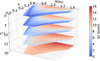 |
Fig. 1 Orbital dissimilarity metric across the a–e–i parameter space. Bluer colors indicate higher degrees of orbital similarity. |
2.3 Calculation of L/T
Regarding the distribution of lunar crater density, many previous studies have provided theoretical expressions (e.g., Zahnle et al. 2001; Le Feuvre & Wieczorek 2011; Wang & Zhou 2016). While there are slight quantitative differences in the formulas presented in these works, they are qualitatively consistent overall. The central point of the leading hemisphere of the Moon (90°W, 0°) is commonly referred to as the apex, while the (90°E, 0°) is termed the antapex. According to Wang & Zhou (2016), when considering only the leading-trailing asymmetry, the crater density Nc at a given lunar surface location can be approximated as
![Mathematical equation: $\[N_c=A_0\left(1+A_1 \cos (\beta)\right),\]$](/articles/aa/full_html/2026/05/aa59075-26/aa59075-26-eq8.png) (2)
(2)
where A0 represents the average crater density over the entire lunar surface, A1 quantifies the degree of leading-trailing asymmetry, and β denotes the spherical distance of the point from the apex. According to Eq. (2), the crater density ratio between the apex and antapex is (1 + A1)/(1 − A1). Integrating Eq. (2) over the entire lunar surface further yields the L/T as (2 + A1)/(2 − A1). Evidently, the latter ratio is slightly smaller than the former. Both ratios have been employed in previous studies; in this work, we utilize the latter ratio as an indicator. For studies reporting apexantapex density ratios, we converted them to the L/T to enable consistent comparisons.
In our simulations, the probability of small bodies impacting the Moon is significantly lower than the probability of them impacting Earth. To enhance the statistical significance of the results, we did not directly track the positions of lunar impacts; instead, we considered all impacts on both the Earth and the Moon as “potential lunar impactors.” We recorded the relative velocity of two objects at the time of impact (vimp) for each collision and used this information to deduce the venc of the small body. For small bodies that collide with the Earth, the expression is ![Mathematical equation: $\[v_{enc}=\sqrt{v_{i m p}^{2}-\frac{2 G M_{E}}{R_{E}}+\frac{2 G M_{E}}{R_{H}}}\]$](/articles/aa/full_html/2026/05/aa59075-26/aa59075-26-eq9.png) , where G, ME, RE, and RH represent the gravitational constant, Earth’s mass, Earth’s radius, and Earth’s Hill radius, respectively. In this scenario, the influence of lunar gravity is neglected. On the other hand, for small bodies colliding with the Moon, the acceleration effect of Earth’s gravity is taken into account. In this case, the expression for the encounter velocity is
, where G, ME, RE, and RH represent the gravitational constant, Earth’s mass, Earth’s radius, and Earth’s Hill radius, respectively. In this scenario, the influence of lunar gravity is neglected. On the other hand, for small bodies colliding with the Moon, the acceleration effect of Earth’s gravity is taken into account. In this case, the expression for the encounter velocity is ![Mathematical equation: $\[v_{enc}=\sqrt{v_{imp}^{2}-\frac{2 G M_{M}}{R_{M}}-\frac{2 G M_{E}}{a_{M}}+\frac{2 G M_{E}}{R_{H}}}\]$](/articles/aa/full_html/2026/05/aa59075-26/aa59075-26-eq10.png) , where MM, RM, and aM represent the Moon’s mass, Moon’s radius, and the semimajor axis of the Moon’s orbit around the Earth, respectively.
, where MM, RM, and aM represent the Moon’s mass, Moon’s radius, and the semimajor axis of the Moon’s orbit around the Earth, respectively.
After calculating the venc of a small body, we can further derive the expected values of impacts on the leading and trailing sides of the Moon. Wang & Zhou (2016) have developed a theoretical model for lunar crater distribution under a planar approximation (neglecting Earth and Moon gravity), from which we can approximate ![Mathematical equation: $\[A_{1} \propto \frac{v_{M}}{v_{enc}}\]$](/articles/aa/full_html/2026/05/aa59075-26/aa59075-26-eq11.png) . If focusing solely on crater number density, the proportionality constant is π/2; when accounting for the higher relative impact velocities (and thus larger crater sizes) on the leading side, the expression becomes
. If focusing solely on crater number density, the proportionality constant is π/2; when accounting for the higher relative impact velocities (and thus larger crater sizes) on the leading side, the expression becomes
![Mathematical equation: $\[A_1=\frac{\pi^2+\left(16-\pi^2\right) \gamma_p \alpha_p}{2 \pi} \frac{v_M}{v_{e n c}},\]$](/articles/aa/full_html/2026/05/aa59075-26/aa59075-26-eq12.png) (3)
(3)
where γp and αp represent parameters associated with crater formation and size distribution. With typical values, the coefficient in Eq. (3) is approximately 2.53. Therefore, in this study, we adopted ![Mathematical equation: $\[A_{1}=2.53 \frac{v_{M}}{v_{e n c}}\]$](/articles/aa/full_html/2026/05/aa59075-26/aa59075-26-eq13.png) to calculate the L/T.
to calculate the L/T.
Equation (3) is utilized to calculate the expected probability of a small body impacting the leading and trailing sides. When computing the overall L/T for numerous objects, we count the expected impacts for both sides separately and then take their ratio. In cases where a small body’s velocity is extremely slow such that A1 > 2, we no longer apply the formula; instead, we assume the body will inevitably impact the leading side. Additionally, there are rare instances where the calculation of venc yields a negative value under the square root. This typically occurs when the small body has experienced significant deceleration due to Earth’s or Moon’s gravity prior to impact. For such cases, we likewise consider the impact to be certain on the leading side.
3 Results
3.1 Distinct orbits of escaped lunar ejecta
Generally speaking, a significant portion of lunar ejecta will directly fall back onto the lunar surface and create craters. Due to the relatively slow impact velocities, these secondary craters typically have lower depth-to-diameter ratios and smaller sizes; thus, most of them have not been counted in previous statistics (e.g., Morota & Furumoto 2003; Kawamura et al. 2011; Williams et al. 2018; Zhao et al. 2024). In this study, we focus primarily on ejecta that can escape the gravitational influence of the Earth-Moon system. Consequently, our analysis considers only collisions and distributions of ejecta 100 yr after the initial moment when they started from 2 radii distance. This timescale allows for the clearance of non-escaping material, while remaining short enough that most ejecta in heliocentric orbits have not yet experienced significant perturbations or re-impacts. Figure 2 presents the distribution of the a, e, i, and Δv for the simulated ejecta population at t = 100 yr.
As shown in Fig. 2, ejecta with lower v0 remain closer to Earth-like orbits (smaller e and i, a ~ 1 au), resulting in a lower Δv. In contrast, ejecta with higher v0 populate a broader range of orbital elements, achieving higher Δv values. The maximum Δv attainable is approximately equal to their v0, demonstrating that initial conditions imprint a lasting kinematic memory.
Moreover, when examining the three-dimensional (3D) trajectories of the ejecta, we notice that these trajectories almost converge at a single point in space. This point corresponds to the initial position of the Earth-Moon system in the simulation, which is where the ejecta were released. This configuration implies that whenever Earth approaches this point, the impact flux on both Earth and Moon would increase significantly. As this phenomenon repeats annually, it bears resemblance to meteor showers. Because of the orbital precession, the ejecta gradually disperse throughout the vast space near the Earth. Consequently, this orbital focusing effect can only persist for a limited duration, typically on the order of 103 to 104 yr.
In Fig. 2, distinct vertical gaps can be observed, which are induced by the Earth’s mean-motion resonances (MMRs). The most prominent MMRs include: the 1:1 MMR at 1 au, the 2:3 MMR at 1.31 au, and the 3:4 MMR at 1.21 au, along with numerous higher order MMRs that are also visibly present. This indicates that Earth’s gravity constitutes the dominant mechanism influencing lunar ejecta, with significant effects already manifesting within a mere 100 yr timescale.
Another intriguing question concerns how the initial location and ejection time of lunar ejecta influence their orbital characteristics, which we explore in the next part. First, in Fig. 3, we present the relationship between the orbits of lunar ejecta and their initial positions under three different values of v0.
Figure 3 indicates that at lower v0, the orbital characteristics of ejecta show minimal variation regardless of release position, as they all occupy Earth-like orbits with low-e and low-i. However, for faster v0, the release position exerts progressively greater influence on the final orbital parameters. In particular, i is largely determined by their latitude of ejection.
When v0 = 2 km/s, it is evident that many small bodies in the trailing side of the Moon do not survive to 100 yr. This phenomenon occurs because v0 is defined relative to the Moon, while the ejecta from the leading side has a higher relative velocity with respect to Earth, making it more likely to escape Earth’s gravitational influence. In the right panel of Fig. 3, the Δv of the ejecta are primarily affected by their v0. However, for the same v0, an asymmetry is noted between the leading and trailing sides, with objects ejected from the leading side generally exhibiting higher Δv.
For the cases where v0 > 2 km/s, apart from some ejecta initially directed towards Earth (located near (20°E, 0°), with exact coordinates varying slightly with v0), nearly all the ejecta can escape Earth’s gravitational influence and survive for over 100 yr. Furthermore, ejecta trajectories passing closer to Earth will be significantly affected by the scattering effect, manifesting as combinations of higher i and lower e.
On the other hand, the lunar phase at the time of ejecta launch also influences the simulation outcomes. To investigate this, we first defined the phase angle, ϕ, as the Sun-Earth-Moon angle. We selected four time instances near the initial epoch of our primary simulation: MJD 59988.7, MJD 59995.3, MJD 60002.3, and MJD 60010.5. At these epochs, the ϕ approximates 270°, 0°, 90°, and 180°, respectively. We set the v0 of the ejecta as 3 km/s and examined the orbital differences of ejecta launched at these distinct times. The corresponding relationship is presented in Fig. 4. Obviously, the distribution of the inclination is basically not affected at all by the lunar phase.
In Fig. 4, the most apparent pattern is that the semimajor axes and eccentricities of small bodies are significantly influenced by the lunar phase. Ejecta launched at low latitudes and in directions perpendicular to the Sun (i.e., aligned with or opposite to Earth’s orbital motion) tend to exhibit higher eccentricities. Among them, ejecta launched in the direction aligned with Earth’s motion acquire both higher eccentricities and larger semimajor axes, while those launched opposite to Earth’s motion are predominantly distributed on the inner side of Earth’s orbit.
In addition to the velocity superposition effect caused by Earth’s orbital motion, the Moon’s revolution around Earth also leads to systematically higher eccentricities for ejecta released from the leading side. When the Moon moves in the same direction as Earth’s orbital motion (ϕ = 180°), the two mechanisms reinforce each other. Ejecta from the leading side exhibit the highest eccentricities and most ejecta are distributed outside Earth’s orbit. Conversely, when the Moon moves opposite to Earth’s direction (ϕ = 0°), the effects partially cancel out, resulting in a notable reduction of high-eccentricity ejecta and causing most projectiles to fall inside Earth’s orbit. In general, the average Δv at ϕ = 180° is approximately 26% higher than at ϕ = 0°.
The above discussion on lunar phases indicates that although our main initial epoch (MJD 60000.0) was arbitrarily selected, the ϕ = 62.5° at this time implies that the directions of Earth’s and the Moon’s motions were neither fully aligned nor opposed. This configuration ensures that the orbital distribution of lunar ejecta launched at this epoch retains a certain degree of representativeness. Furthermore, while our tests were conducted only at v0 = 3 km/s, it is anticipated that the influence of lunar phase would be relatively diminished at higher v0. Additionally, the probability of impact events on the Moon may also vary slightly with lunar phase, suggesting that the quantity of ejecta emitted could also differ across phases. This mechanism warrants further investigation in future work.
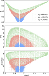 |
Fig. 2 Distributions of a, e, i, and Δv of simulated ejecta at t = 100 yr. Points of different colors represent ejecta with different v0 values. |
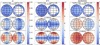 |
Fig. 3 Relationship between the orbits of lunar ejecta and their initial positions at different v0. From left to right, the panels represent e, i, and Δv, respectively. Blank areas indicate ejecta that did not survive until t = 100 yr in the simulations. Black lines mark the lunar latitude and longitude grid, with longitude intervals of 45° and latitude intervals of 30°. |
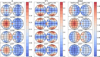 |
Fig. 4 Similar to Fig. 3, but the right column represents the semimajor axes of the ejecta and panels from top to bottom represent different lunar phases. In the plots, the v0 of all lunar ejecta is 3 km/s. The open yellow and red circles mark the directions of Earth and the Sun, as viewed from the Moon, respectively. |
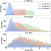 |
Fig. 5 Δv distributions at 100 yr, 100 kyr, and 1 Myr. Different colors representing distinct v0. Only three values are plotted for clarity. |
3.2 Long-term orbital excitation
The subsequent evolution of lunar ejecta over million-year timescales shows progressive orbital excitation. In Fig. 5, we present the Δv distributions of lunar ejecta at three different times to illustrate their dynamical evolution.
The middle panel of Fig. 5 reveals that after 100 kyr of evolution, although the quantity of surviving ejecta has decreased significantly, the average Δv has increased only marginally, and differences among populations with different v0 remain observable. However, the velocity distribution has undergone substantial changes, exhibiting a Rayleigh-like distribution pattern with an emergent population of higher Δv objects. By 1 Myr, the initially distinct Δv distributions for different v0 populations become largely indistinguishable, converging toward an average Δv of ~5 km/s. However, it is noteworthy that these ejecta are still much slower than typical NEOs even after 1 Myr.
This evolution follows a characteristic pattern: ejecta launched with low-velocities experience rapid depletion due to early collisions, while higher-velocity populations have longer lifetime but lower initial impact probabilities. The timescale for complete orbital randomization is approximately 1 Myr, after which the dynamical memory of initial conditions becomes negligible.
As the orbits of the ejecta become progressively excited, both their flux and velocity upon returning to the Earth–Moon system are consequently affected. Our simulations recorded substantial impact events on terrestrial planets, with Earth receiving the majority (67.33%), followed by Venus (31.15%) and the Moon (0.83%). Based on the recorded impact events, we calculated the venc of the objects upon entering the Hill radius of the Earth-Moon system. This velocity was subsequently used to estimate the probability of impacts on the leading versus trailing hemisphere of the Moon. Figure 6 illustrates the impact time and the distribution of venc for the collision events on the Earth and the Moon.
The temporal distribution of impacts reveals distinct phases of ejecta evolution. The initial phase (<10 kyr) shows minimal velocity evolution, with venc closely reflecting initial conditions. Low-velocity ejecta (v0 = 2 km/s) dominate this early impact flux. On the other hand, a strong correlation exists between venc and v0, showing that impactors returning to the Earth-Moon system within this phase partly retain kinematic memory of their launch conditions.
The timescale for the orbital excitation of ejecta is ~100 kyr, during which the venc gradually increases. Beyond 1 Myr, the venc distribution becomes homogeneous across all v0 groups. This velocity evolution is directly correlated with the Δv progression shown in Fig. 5, confirming the consistency between these two metrics as diagnostic indicators of impactor dynamics.
3.3 Impact flux and the L/T
In this study, we individually simulated scenarios across different v0 values and subsequently integrated their results through fitting and weighting procedures to derive comprehensive conclusions. Here, we summarize the basic information from several simulations in Table 1. As shown in the second row of Table 1, vL is derived from v0 (when the ejecta is located at twice the lunar radius). The third row presents the launch frequency, which follows a power-law distribution proportional to ![Mathematical equation: $\[v_{L}^{-4}\]$](/articles/aa/full_html/2026/05/aa59075-26/aa59075-26-eq14.png) (Jiao et al. 2024), with normalization such that the relative frequency equals 1 when vL = 2.38 km/s (the Moon’s escape velocity). Row 4 reports the successful escape counts, referring to the surviving ejecta population at t = 100 yr.
(Jiao et al. 2024), with normalization such that the relative frequency equals 1 when vL = 2.38 km/s (the Moon’s escape velocity). Row 4 reports the successful escape counts, referring to the surviving ejecta population at t = 100 yr.
As our primary focus is on the ejecta that have the capacity to escape the Earth-Moon system’s Hill radius, Table 1 reveals that the probability of ejecta failing to escape can be well-fitted with an exponential function. Meanwhile, the probability of escaping can be expressed as Pescape = 1–9139.4 exp(−4.1vL), as shown by the blue line in Fig. 7. Thus, the population of successfully escaped ejecta follows the distribution ![Mathematical equation: $\[f\left(v_{L}\right)=45.83 v_{L}^{-4}(1- \left.9139.4 \exp \left(-4.1 v_{L}\right)\right)\]$](/articles/aa/full_html/2026/05/aa59075-26/aa59075-26-eq15.png) , where the coefficient 45.83 ensures that the integral of this function from 2.38 to infinity equals 1. This f(vL) serves as the weighting function for all subsequent calculations of impact flux, venc, and L/T.
, where the coefficient 45.83 ensures that the integral of this function from 2.38 to infinity equals 1. This f(vL) serves as the weighting function for all subsequent calculations of impact flux, venc, and L/T.
From Fig. 6, it is evident that small bodies with different v0 values exhibit varying decay timescales for their impact frequencies. Slow ejecta tend to produce numerous impacts during the early phase, but their collision frequency decays rapidly, while fast ejecta behave in the opposite way. Through empirical testing, we find that the cumulative number of Earth-Moon system impacts at a given time t, denoted as C(t), can be well described by
![Mathematical equation: $\[C(t)=m\left(1-\exp \left(\frac{-c t^k}{m}\right)\right).\]$](/articles/aa/full_html/2026/05/aa59075-26/aa59075-26-eq16.png) (4)
(4)
The derivative of Eq. (4) is given by ![Mathematical equation: $\[\frac{d C(t)}{d t}=c k t^{k-1} ~\exp \left(\frac{-c t^{k}}{m}\right)\]$](/articles/aa/full_html/2026/05/aa59075-26/aa59075-26-eq17.png) , and for small t, the collision rate is
, and for small t, the collision rate is ![Mathematical equation: $\[\frac{d C(t)}{d t} \approx c k t^{k-1}\]$](/articles/aa/full_html/2026/05/aa59075-26/aa59075-26-eq18.png) . Here, parameter c governs the baseline collision frequency, while k is a value between 0 and 1 that characterizes the decay of the function. Consequently, at early simulation times, the cumulative impact count approximately follows a power law C(t) ≈ ctk, which aligns with the typical functional form (e.g., Castro-Cisneros et al. 2025a). However, a simple power function does not converge as t → ∞. To account for finite ejecta populations and improve late-stage fitting accuracy, an additional parameter m is introduced. This modification ensures that for large t, C(t) asymptotically approaches m from below. In Fig. 8, we illustrate the evolution of the C(t) over time for different v0, along with the fitting results from Eq. (4).
. Here, parameter c governs the baseline collision frequency, while k is a value between 0 and 1 that characterizes the decay of the function. Consequently, at early simulation times, the cumulative impact count approximately follows a power law C(t) ≈ ctk, which aligns with the typical functional form (e.g., Castro-Cisneros et al. 2025a). However, a simple power function does not converge as t → ∞. To account for finite ejecta populations and improve late-stage fitting accuracy, an additional parameter m is introduced. This modification ensures that for large t, C(t) asymptotically approaches m from below. In Fig. 8, we illustrate the evolution of the C(t) over time for different v0, along with the fitting results from Eq. (4).
Since we previously accounted for the escape probability of ejecta, in this fitting procedure, we normalized the impact count for each v0 group by dividing it by the corresponding escape probability; namely, by assuming 10 000 small bodies of each v0 successfully escape the Earth-Moon system. According to Eq. (4), the number of ejecta impacting the Earth-Moon system between t0 and t1 is given by
![Mathematical equation: $\[C\left(t_1\right)-C\left(t_0\right)=\int_{2.38}^{\infty} f\left(v_L\right) \times\left(C\left(v_L, t_1\right)-C\left(v_L, t_0\right)\right) d v_L.\]$](/articles/aa/full_html/2026/05/aa59075-26/aa59075-26-eq19.png) (5)
(5)
At this step, all parameters (c, k, and m) in Eq. (4) are fitted as a sigmoid function of vL. Consequently, in Eq. (4), we express the cumulative impact count as a function of both vL and t. In Fig. 8, the cumulative impact count integrated over different vL is represented by the black dashed line. When calculating the L/T from t0 to t1, we further need to fit the L/T as a function of vL. Therefore, the overall L/T during this period can be expressed as
![Mathematical equation: $\[\frac{L\left(t_1\right)-L\left(t_0\right)}{T\left(t_1\right)-T\left(t_0\right)}=\frac{\int_{2.38}^{\infty} f\left(v_L\right) \times\left(C\left(v_L, t_1\right)-C\left(v_L, t_0\right)\right) \times \frac{L / T\left(v_L\right)}{1+L / T\left(v_L\right)} d v_L}{\int_{2.38}^{\infty} f\left(v_L\right) \times\left(C\left(v_L, t_1\right)-C\left(v_L, t_0\right)\right) \times \frac{1}{1+L / T\left(v_L\right)} d v_L},\]$](/articles/aa/full_html/2026/05/aa59075-26/aa59075-26-eq20.png) (6)
(6)
where L(t) and T(t) represent the cumulative impacts received by the leading side and trailing side respectively up to the time, t.
Based on the above methodology, we calculated the flux and venc of lunar ejecta with different v0 for collisions on the Earth-Moon system across various time intervals, as well as the resulting L/T, as shown in Table 2. Using Eqs. (5) and (6), we summarize the weighted aggregate results in the final column. We note that while the upper limits of integration in Eqs. (5) and (6) are set to infinity, in practical computations, this upper bound is truncated at 10 km/s. This cutoff ensures the inclusion of the vast majority of lunar ejecta and faster ejecta do not significantly influence the results presented in this study.
The last column of Table 2 reveals that approximately 25% of ejecta will return to the Earth-Moon system by impact within 3 Myr, with an overall venc of about 2.26 km/s and an overall L/T of about 5.9, indicating the leading hemisphere experiences nearly six times more impacts than the trailing side. Notably, about half of these collisions occur within the first 100 kyr. The L/T shows strong time dependence, decreasing from extremely high values (>20) during the initial 10 kyr to approximately 2.0 after 1 Myr.
As shown by Table 1, roughly 1.22% of ejecta that returned to the Earth-Moon system ultimately impacted the Moon. For every 10 000 escaped ejecta, we projected approximately 30.6 lunar impacts, distributed as 26.2 on the leading side and 4.4 on the trailing side. This pronounced asymmetry stems from the low venc of re-impacting ejecta.
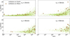 |
Fig. 6 Distribution of time and venc for collision events on Earth–Moon system. The x-axis represents time on a logarithmic scale, while the y-axis shows the venc, which indicates the velocities of impactors as they enter the Hill radius of the Earth–Moon system. For clarity, impacts on the Moon are highlighted with larger markers. |
Proportion of ejecta at different v0 and the total number of collisions.
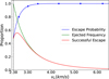 |
Fig. 7 Relationship between the proportion of ejecta escaping the Earth-Moon system and their vL. The launch frequency is provided by Jiao et al. (2024), while the escape probability is derived from simulation results (represented by blue points). The dashed line on the left indicates the Moon’s escape velocity. |
Impact characteristics across different v0 and different time intervals.
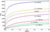 |
Fig. 8 Cumulative impact count of lunar ejecta on the Earth-Moon system as a function of time. The light-colored points represent the simulated cumulative impact counts, while the solid lines correspond to the fitted results based on Eq. (4). The black dashed line represents the overall result obtained after weighting different v0. |
4 Conclusion and discussion
Our simulations support the idea that re-impacting lunar ejecta constitute a population of low-velocity impactors capable of generating an extreme leading-trailing asymmetry (L/T ≈ 5.9). This finding provides a direct solution to the long-standing discrepancy between the observed lunar crater distribution (L/T ≈ 1.4–1.9; e.g., Morota & Furumoto 2003; Oberst et al. 2012; Kawamura et al. 2011; Williams et al. 2018) and theoretical models based solely on NEO impactors (L/T ≈ 1.14; e.g., Gallant et al. 2009; Ito & Malhotra 2010; Le Feuvre & Wieczorek 2011; Wang & Zhou 2016). By considering a mixed impactor population, we find that if lunar ejecta contribute approximately 15.4% of the total impactors, the resulting net L/T ratio aligns with the observed value of ~1.4. This implies that on the leading hemisphere, ejecta re-impacts could account for nearly 23% of craters, underscoring their disproportionate role in shaping the asymmetric surface record.
Furthermore, the exceptionally high L/T ratio of 3.11 observed during the Imbrian-Nectarian period (Zhao et al. 2024) could be explained if ejecta did indeed comprise up to ~70% of impactors. Such a higher proportion might indicate that large impact events were relatively frequent and violent during that period, generating a substantial amount of lunar ejecta. It should be noted that the required proportion of lunar ejecta would be somewhat overestimated when we take into account the fact that the Moon’s orbital semimajor axis was smaller at that time.
The potential significance of lunar ejecta as a major impactor source can benefit from indirect support coming from meteorite studies. Many meteorites found on Earth do not exhibit spectral similarities to typical NEOs or main-belt asteroids (e.g., Vernazza et al. 2008; de León et al. 2010). Recent research suggests that most meteorites originate from a limited number of parent bodies and collision events (e.g., Brož et al. 2024; Granvik 2024; Marsset et al. 2024). This aligns with our model, in which a single lunar impact could generate much debris that influence the Earth-Moon system’s impact flux over millions of years. The stochastic nature of such events could explain temporal variations in the impactor population and the resulting cratering asymmetry.
In previous studies, when impactors were assumed to be NEOs, the estimated proportion of lunar impacts relative to the total Earth-Moon system was approximately 4.7% (Ito & Malhotra 2010). In additon, theoretical studies on lunar meteoroid impacts have suggested a lunar contribution of about 3.1% (Pokorný et al. 2019). However, a critical finding of our study is the low probability (~1.2%) of a returning ejecta fragment ultimately impacting the Moon. This discrepancy is not a numerical artifact, but a fundamental physical outcome dictated by gravitational focusing. The collisional cross-section of a planet scales with ![Mathematical equation: $\[b=\sqrt{R^{2}+\frac{2 G M R}{v^{2}}}\]$](/articles/aa/full_html/2026/05/aa59075-26/aa59075-26-eq24.png) , where v is the velocity of impactor and R and M are the radius and mass of the target body. For high-velocity objects, the lunar impact probability approaches the geometric ratio of the Moon’s cross-sectional area to that of the Earth-Moon system (6.9%). However, for low-velocity impactors, the gravitational focusing term
, where v is the velocity of impactor and R and M are the radius and mass of the target body. For high-velocity objects, the lunar impact probability approaches the geometric ratio of the Moon’s cross-sectional area to that of the Earth-Moon system (6.9%). However, for low-velocity impactors, the gravitational focusing term ![Mathematical equation: $\[\frac{2 G M R}{v^{2}}\]$](/articles/aa/full_html/2026/05/aa59075-26/aa59075-26-eq25.png) becomes dominant, dramatically increasing Earth’s collisional cross section relative to the Moon’s. Consequently, the Moon’s share of impacts drops to ~1.5% at v = 5 km/s. This mechanism inherently suppresses the proportion of lunar impact for low-velocity ejecta, a factor that must be considered when estimating the absolute flux of lunar ejecta required to explain the observed cratering record.
becomes dominant, dramatically increasing Earth’s collisional cross section relative to the Moon’s. Consequently, the Moon’s share of impacts drops to ~1.5% at v = 5 km/s. This mechanism inherently suppresses the proportion of lunar impact for low-velocity ejecta, a factor that must be considered when estimating the absolute flux of lunar ejecta required to explain the observed cratering record.
The size distribution of ejecta fragments introduces another layer of complexity. Our results, combined with observational trends, suggest that the L/T ratio may be size-dependent. Lunar seismic data, corresponding to craters range from several meters to several tens of meters in diameter, exhibit a more pronounced leading-trailing asymmetry (Kawamura et al. 2011) compared to radial crater data, which reveal sizes of several kilometers across (Morota & Furumoto 2003). Similarly, cold spot data reveal that smaller cold spots show a higher degree of asymmetry (Williams et al. 2018). Moreover, as noted above, the proportion of lunar impacts indicated by lunar meteorites (Pokorný et al. 2019) is lower than that predicted by models using NEOs impactors (Ito & Malhotra 2010), suggesting that smaller meteorite impacts may involve lower velocities, consequently resulting in a higher cratering asymmetry.
This size-dependent asymmetry may arise partly because small-sized bodies inherently exhibit different orbital distributions and the lunar ejecta discussed in this study likely contribute significantly to this phenomenon. However, larger ejecta fragments tend to be launched at lower velocities (Singer et al. 2020), which could make them more likely to impact on the leading side. The intricate interplay between impactor source, velocity, and fragment size, along with their temporal evolution, warrants further investigation. On the other hand, nongravitational effects, such as the Yarkovsky effect, may play a prominent role for small-sized objects, potentially leading to outcomes such as the circularization of their orbits (e.g., Spitale & Greenberg 2002). This further confirms that the asymmetric cratering on the lunar surface may be strongly influenced by the size of impactor. In addition to the observational studies mentioned above, some research has also focused on smaller-scale impacts (e.g., Cremonese et al. 2013; Horányi et al. 2015; Szalay & Horányi 2016; Pokorný et al. 2019; Verkercke et al. 2025). The leading-trailing asymmetry resulting from such micro-meteoroid collisions represents another noteworthy issue for future investigation.
This work establishes lunar ejecta as a dynamic population that effectively shapes the lunar impact environment, moving beyond their traditional view as mere geological byproducts. Our quantitative model provides a framework for integrating this component into lunar chronology models and for re-evaluating the impact history of the Earth-Moon system (e.g., Lagain et al. 2024).
However, key uncertainties remain. The absolute production rate of ejecta that escape the Earth-Moon system is highly dependent on the magnitude and frequency of large primary impacts, which are stochastic in nature. Future works should be focused on improving the constraints on this production function across different geological epochs. Additionally, more detailed modeling of impact dynamics will allow for current models to be refined. Future missions, such as China’s Tianwen-2 mission to the potentially lunar-derived asteroid Kamo’oalewa (e.g., Sharkey et al. 2021; Jiao et al. 2024), will provide ground-truth data that can significantly constrain the properties and dynamics of material originating from the Moon.
Acknowledgements
This work is supported by the Science and Technology Development Fund (FDCT) of Macau (grant Nos. 0034/2024/AMJ, 0008/2024/AKP, 002/2024/SKL, 0002/2025/AKP) and the National Key Research and Development Program of China (grant No. 2024YFE0201000). Li-Yong Zhou thanks the support from National Natural Science Foundation of China (NSFC, Grants No. 12373081 & No.12150009) and the China Manned Space Program with grant No.CMS-CSST-2025-A16.
References
- Brož, M., Vernazza, P., Marsset, M., et al. 2024, Nature, 634, 566 [Google Scholar]
- Castro-Cisneros, J. D., Malhotra, R., & Rosengren, A. J. 2023, Commun. Earth Environ., 4, 372 [Google Scholar]
- Castro-Cisneros, J. D., Malhotra, R., & Rosengren, A. J. 2025a, Icarus, 438, 116606 [Google Scholar]
- Castro-Cisneros, J. D., Malhotra, R., & Rosengren, A. J. 2025b, Icarus, 429, 116379 [NASA ADS] [CrossRef] [Google Scholar]
- Cremonese, G., Borin, P., Lucchetti, A., Marzari, F., & Bruno, M. 2013, A&A, 551, A27 [NASA ADS] [CrossRef] [EDP Sciences] [Google Scholar]
- de León, J., Licandro, J., Serra-Ricart, M., Pinilla-Alonso, N., & Campins, H. 2010, A&A, 517, A23 [CrossRef] [EDP Sciences] [Google Scholar]
- Fenucci, M., Gronchi, G. F., & Novaković, B. 2023, A&A, 672, A39 [NASA ADS] [CrossRef] [EDP Sciences] [Google Scholar]
- Gallant, J., Gladman, B., & Ćuk, M. 2009, Icarus, 202, 371 [Google Scholar]
- Gladman, B. J., Burns, J. A., Duncan, M. J., & Levison, H. F. 1995, Icarus, 118, 302 [NASA ADS] [CrossRef] [Google Scholar]
- Granvik, M. 2024, Nature, 634, 553 [Google Scholar]
- Halliday, I. 1964, Meteoritics, 2, 271 [Google Scholar]
- Halliday, I., & Griffin, A. A. 1982, Meteoritics, 17, 31 [Google Scholar]
- Horányi, M., Szalay, J. R., Kempf, S., et al. 2015, Nature, 522, 324 [CrossRef] [Google Scholar]
- Horedt, G. P., & Neukum, G. 1984, Icarus, 60, 710 [NASA ADS] [CrossRef] [Google Scholar]
- Housen, K. R., & Holsapple, K. A. 2011, Icarus, 211, 856 [NASA ADS] [CrossRef] [Google Scholar]
- Ito, T., & Malhotra, R. 2010, A&A, 519, A63 [NASA ADS] [CrossRef] [EDP Sciences] [Google Scholar]
- Jiao, Y., Cheng, B., Huang, Y., et al. 2024, Nat. Astron., 8, 819 [NASA ADS] [CrossRef] [Google Scholar]
- Kawamura, T., Morota, T., Kobayashi, N., & Tanaka, S. 2011, Geophys. Res. Lett., 38, L15201 [Google Scholar]
- Lagain, A., Devillepoix, H. A. R., Vernazza, P., et al. 2024, Icarus, 411, 115956 [Google Scholar]
- Le Feuvre, M., & Wieczorek, M. A. 2011, Icarus, 214, 1 [Google Scholar]
- Li, H.-C., Zhang, N., Yue, Z.-Y., & Zhang, Y.-Z. 2021, Res. Astron. Astrophys., 21, 140 [Google Scholar]
- Malhotra, R. 2019, Nat. Astron., 3, 193 [Google Scholar]
- Marsset, M., Vernazza, P., Brož, M., et al. 2024, Nature, 634, 561 [Google Scholar]
- Michel, P., & Froeschlé, C. 1997, Icarus, 128, 230 [NASA ADS] [CrossRef] [Google Scholar]
- Morota, T., & Furumoto, M. 2003, Earth Planet. Sci. Lett., 206, 315 [Google Scholar]
- Oberst, J., Christou, A., Suggs, R., et al. 2012, Planet. Space Sci., 74, 179 [Google Scholar]
- Pinet, P. 1985, A&A, 151, 222 [Google Scholar]
- Pokorný, P., Janches, D., Sarantos, M., et al. 2019, J. Geophys. Res. (Planets), 124, 752 [Google Scholar]
- Schenk, P. M., & Sobieszczyk, S. 1999, in Bulletin of the American Astronomical Society, 31, 1182 [Google Scholar]
- Sfair, R., Gomes, L. C., Winter, O. C., et al. 2025, Open J. Astrophys., 8, 136 [Google Scholar]
- Sharkey, B. N. L., Reddy, V., Malhotra, R., et al. 2021, Commun. Earth Environ., 2, 231 [NASA ADS] [CrossRef] [Google Scholar]
- Singer, K. N., Jolliff, B. L., & McKinnon, W. B. 2020, J. Geophys. Res. (Planets), 125, e06313 [Google Scholar]
- Spitale, J., & Greenberg, R. 2002, Icarus, 156, 211 [NASA ADS] [CrossRef] [Google Scholar]
- Szalay, J. R., & Horányi, M. 2016, Geophys. Res. Lett., 43, 4893 [NASA ADS] [CrossRef] [Google Scholar]
- Verkercke, S., Senel, C. B., Luther, R., et al. 2025, J. Geophys. Res. (Planets), 130, e2025JE009259 [Google Scholar]
- Vernazza, P., Binzel, R. P., Thomas, C. A., et al. 2008, Nature, 454, 858 [NASA ADS] [CrossRef] [Google Scholar]
- Wang, N., & Zhou, J.-L. 2016, A&A, 594, A52 [NASA ADS] [CrossRef] [EDP Sciences] [Google Scholar]
- Werner, S. C., & Medvedev, S. 2010, Earth Planet. Sci. Lett., 295, 147 [Google Scholar]
- Williams, J. P., Bandfield, J. L., Paige, D. A., et al. 2018, J. Geophys. Res. (Planets), 123, 2380 [Google Scholar]
- Wood, J. A. 1973, Moon, 8, 73 [Google Scholar]
- Zahnle, K., Dones, L., & Levison, H. F. 1998, Icarus, 136, 202 [NASA ADS] [CrossRef] [Google Scholar]
- Zahnle, K., Schenk, P., Sobieszczyk, S., Dones, L., & Levison, H. F. 2001, Icarus, 153, 111 [NASA ADS] [CrossRef] [Google Scholar]
- Zhao, C., Yue, Z., Di, K., et al. 2024, Planet. Space Sci., 254, 106015 [Google Scholar]
All Tables
All Figures
|
Fig. 1 Orbital dissimilarity metric across the a–e–i parameter space. Bluer colors indicate higher degrees of orbital similarity. |
| In the text | |
|
Fig. 2 Distributions of a, e, i, and Δv of simulated ejecta at t = 100 yr. Points of different colors represent ejecta with different v0 values. |
| In the text | |
|
Fig. 3 Relationship between the orbits of lunar ejecta and their initial positions at different v0. From left to right, the panels represent e, i, and Δv, respectively. Blank areas indicate ejecta that did not survive until t = 100 yr in the simulations. Black lines mark the lunar latitude and longitude grid, with longitude intervals of 45° and latitude intervals of 30°. |
| In the text | |
|
Fig. 4 Similar to Fig. 3, but the right column represents the semimajor axes of the ejecta and panels from top to bottom represent different lunar phases. In the plots, the v0 of all lunar ejecta is 3 km/s. The open yellow and red circles mark the directions of Earth and the Sun, as viewed from the Moon, respectively. |
| In the text | |
|
Fig. 5 Δv distributions at 100 yr, 100 kyr, and 1 Myr. Different colors representing distinct v0. Only three values are plotted for clarity. |
| In the text | |
|
Fig. 6 Distribution of time and venc for collision events on Earth–Moon system. The x-axis represents time on a logarithmic scale, while the y-axis shows the venc, which indicates the velocities of impactors as they enter the Hill radius of the Earth–Moon system. For clarity, impacts on the Moon are highlighted with larger markers. |
| In the text | |
|
Fig. 7 Relationship between the proportion of ejecta escaping the Earth-Moon system and their vL. The launch frequency is provided by Jiao et al. (2024), while the escape probability is derived from simulation results (represented by blue points). The dashed line on the left indicates the Moon’s escape velocity. |
| In the text | |
|
Fig. 8 Cumulative impact count of lunar ejecta on the Earth-Moon system as a function of time. The light-colored points represent the simulated cumulative impact counts, while the solid lines correspond to the fitted results based on Eq. (4). The black dashed line represents the overall result obtained after weighting different v0. |
| In the text | |
Current usage metrics show cumulative count of Article Views (full-text article views including HTML views, PDF and ePub downloads, according to the available data) and Abstracts Views on Vision4Press platform.
Data correspond to usage on the plateform after 2015. The current usage metrics is available 48-96 hours after online publication and is updated daily on week days.
Initial download of the metrics may take a while.