| Issue |
A&A
Volume 709, May 2026
|
|
|---|---|---|
| Article Number | A137 | |
| Number of page(s) | 7 | |
| Section | The Sun and the Heliosphere | |
| DOI | https://doi.org/10.1051/0004-6361/202659348 | |
| Published online | 12 May 2026 | |
Prominence signatures in the Fraunhofer G-band
Testing ionization memory with multi-line prominence diagnostics
1
Leibniz-Institut für Astrophysik Potsdam (AIP), An der Sternwarte 16, 14482 Potsdam, Germany
2
Independent Researcher, Cluj-Napoca, Romania
3
Universität Potsdam, Institut für Physik und Astronomie, Karl-Liebknecht-Straße 24/25, 14476 Potsdam, Germany
★ Corresponding author: This email address is being protected from spambots. You need JavaScript enabled to view it.
Received:
6
February
2026
Accepted:
12
April
2026
Abstract
Context. The Fraunhofer G-band around 4304 Å is widely used as a photospheric diagnostic and is generally not expected to show signatures of chromospheric or coronal structures. However, recent amateur observations have suggested the presence of off-limb prominence emission in this spectral region.
Aims. We investigated the origin of the prominence emission in the G-band to determine whether this is caused by methylene (CH) or other lines in this band. We also tested these lines for the presence of ionization memory effects in neutral lines.
Methods. We present a case study of two prominences, one obtained with a Solar Explorer (Sol’Ex) spectroheliograph, and the other with the high-resolution Fast Multi-Line Universal Spectrograph (FaMuLUS) camera system at the echelle spectrograph of the German Vacuum Tower Telescope (VTT). The line widths were measured for simultaneously observed neutral and ionized metal lines, allowing a comparison of thermal and nonthermal broadening components to determine whether these lines exhibit any ionization memory effects.
Results. We report clear prominence emission in several metal lines within the G-band, primarily from Ti II and Ca I lines, while contributions from CH molecular lines are not observed. A comparison of the simultaneously observed ionized and neutral lines revealed no clear evidence of an ionization memory effect.
Conclusions. Since the prominence emission does not originate from CH lines, we do not call them G-band prominences, but prominences in the G-band, as they are independent of the primary diagnostic in this spectral window. In addition, the absence of a clear ionization memory effect suggests that these effects may be less pronounced for weak neutral lines.
Key words: atomic data / radiative transfer / techniques: spectroscopic / Sun: corona / Sun: photosphere
© The Authors 2026
 Open Access article, published by EDP Sciences, under the terms of the Creative Commons Attribution License (https://creativecommons.org/licenses/by/4.0), which permits unrestricted use, distribution, and reproduction in any medium, provided the original work is properly cited.
This article is published in open access under the Subscribe to Open model. This email address is being protected from spambots. You need JavaScript enabled to view it. to support open access publication.
1. Introduction
The solar G-band is a roughly 10 Å wide spectral band centered around 4304 Å. It is named after the label given by Fraunhofer (1817) in his original spectral classification. This band should not be confused with the much wider Johnson & Morgan (1953) photometric G band, which covers the green part of the spectrum. For this reason, this range is often specifically called the solar G-band, Fraunhofer G-band, or CH band for the many methylidyne lines that are present in this spectral range (e.g., Langhans & Schmidt 2002).
The G-band is dominated by numerous closely spaced rotational-vibrational transitions of the CH molecule, making it a popular diagnostic in high-resolution solar imaging. In cooler regions of the photosphere, such as intergranular lanes, sunspots, and pores, the higher CH abundance leads to enhanced molecular absorption, raising the band’s opacity and lowering the integrated intensity. Conversely, in hotter regions such as granule centers and magnetic flux concentrations (or bright points), the CH molecule is thermally dissociated. This reduces the band opacity, and thus, deeper and hotter layers can contribute to the emergent intensity. This mechanism enhances contrast relative to nearby continuum wavelengths (e.g., Shelyag et al. 2004; Bodnárová et al. 2014; Kamlah et al. 2025). Photospheric imprints of solar flares can also be observed in this band, but only very bright white-light flares, which seem to likewise appear brighter than the surrounding continuum due to the dissociation of the CH molecules (Isobe et al. 2007). In stellar studies, the G-band is used as a probe for the carbon abundance (e.g., Lee et al. 2008).
In summary, the emission from the G-band generally forms in the low to mid photosphere, with its formation height depending on the temperature of the local atmosphere. It is therefore not expected to exhibit signatures of chromospheric phenomena. Nevertheless, informal discussions of the so-called G-band prominence have surfaced in amateur forums and social media groups. The first confirmed detection was posted in August 2024 (Váradi Nagy 2024).
To further investigate these features, a coordinated Professional–Amateur campaign was initiated using a Solar Explorer (Sol’Ex; Buil et al. 2023) spectroheliopgraph, which led to several additional observations (Váradi Nagy 2025). In addition, attempts were made to capture these weak signals in narrow-band photometry, but without success.
Preliminary low-resolution spectra of prominences suggested that the signal primarily originates from emission by metals within the G-band region and not from the CH lines. Therefore, it is more appropriate to refer to them as prominences in the G-band than calling them G-band prominences. However, the low signal-to-noise ratio of these observations does not rule out a contribution from CH absorption features.
We investigated this hypothesis in detail by reprocessing the original Sol’Ex data and conducting and analyzing additional observations with the Fast Multi-Line Universal Spectrograph (FaMuLUS; Denker et al. In prep.) camera system at the echelle spectrograph of the 70 cm German Vacuum Tower Telescope (VTT, Schröter et al. 1985; von der Lühe 1998). We also discuss the diagnostic potential of these lines.
2. Observations and data processing
Two prominences were observed in this work. For each one, we describe the observing instrument, the data processing workflow, and the prominence properties. Context images taken in Hα with the Global Oscillation Network Group (GONG, Harvey et al. 1996) along with the 1600 Å, 304 Å, 171 Å, and 211 Å bands of the Atmospheric Imaging Assembly (AIA, Lemen et al. 2012) on board the Solar Dynamics Observatory (SDO, Pesnell et al. 2012) and shown in Fig. 1.
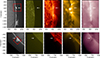 |
Fig. 1. GONG and SDO/AIA observations of two prominences in the Hα, 1600 Å, 304 Å, 171 Å, and 211 Å channels, sampling plasma from the upper chromosphere and transition region to the low corona. The top row shows prominence 1A (observed at 08:47 UT on the 9th of Oktober 2025), located adjacent to an active region, while the bottom row shows prominence 2 (observed at 08:47 on the 11th of November 2025) in a quieter coronal environment. The white arrows indicate the prominence structures in each channel. The red boxes indicate the FOV of the cuts made in the figures below. |
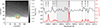 |
Fig. 2. Overview of prominence 1A observations. Left: Prominence 1A imaged in the Ti II 4307.9 Å line (violet line in the right plot) shown in grayscale after the nearby continuum was subtracted (tan line in the right plot). The green contour represents the extent of the prominence in a GONG Hα filtergram. Right: Disk center profile (black) showing the spectral extent of the recording, along with the prominence spectrum (red) after normalization to the disk center continuum intensity. The nine brightest emission lines are marked with dashed vertical lines. The gray shaded region corresponds to the spectral FaMuLUS window. |
2.1. Prominence 1A
The observations of prominence 1A were made with a modified Sol’Ex located in Cluj-Napoca, Romania. The spectroheliograph was attached to a 62/400 refractor, with an aperture stopped down to a diameter of about 4 cm, equipped with a 2-inch Altair solar contrast filter, which was centered at the G-band at 4303 Å with a bandpass of 20 Å and served as an energy rejection filter. The Sol’Ex spectroheliograph has a grating constant of 2400 lines mm−1, which corresponds to a spectral resolving power of  and can be tuned to a wide range of wavelengths (Váradi Nagy & Pietrow 2025). The instrument uses a monochromatic 16-bit Altair Hypercam 26M (APS-C) camera, which can capture weaker signals, but reduces the spectral resolution simultaneously by roughly a factor of two due to its large pixels. The setup can scan the full solar disk in around 4500 slit positions, taking about 1 min. For these observations, the Sol’Ex spectroheliograph was tuned to a spectral window extending from approximately 4298 Å to 4317 Å.
The solar disk was reconstructed and stored as FITS data using the JSol’Ex1 open-source software (Champeau 2026) in the same way as described in Váradi Nagy & Pietrow (2025). The wavelength and intensity were calibrated with the HelioSpectrotron 5000 interactive atlas2 (Pietrow 2026) in combination with the ISPy (Díaz Baso et al. 2021) spectral calibration library and the Neckel & Labs (1984) solar spectral atlas.
Prominence 1A was observed on the west side of the limb at helioprojective Cartesian coordinates (x, y) = (958″, 131″) from 08:29 UT to 11:00 UT on 2025 October 9 (see the white arrow in Fig. 1). During this time period, the prominence remained stable and displayed a relatively strong signal in the Ti II line at 4307.9 Å throughout the time series. We focused on the time period around 10:46 UT because it had the best seeing.
Prominence 1A exhibits by far the strongest G-band signature of all detections observed with this instrument to date (Váradi Nagy 2025). A clear contrast is provided by the prominence located south of prominence 1A (x, y = 960″, −150″), as it appears larger and brighter in Hα and looks more like a typical prominence in the EUV channels, it shows no detectable signature in the Sol’Ex data. We call this structure prominence 1B.
Prominence 1A is detected in multiple AIA channels, but its emission is partly obscured by hot coronal plasma from active region NOAA 14232, which lies along the same line of sight. In AIA 304 Å, it appears comparatively brighter than prominence 1B, indicating enhanced He II emission. It is also visible as a narrow spine in AIA 1600 Å, while no clear signature is detected in AIA 211 Å. A dark triangular shape can be discerned in AIA 171 Å behind the bright active region loops. Nevertheless, the structure appears as an unambiguous prominence in the GONG Hα observations.
The geometry of the system becomes clearer when viewed from the vantage point of the Solar Terrestrial Relation Observatory (STEREO-A, Howard et al. 2008) satellite, which is 48.5° degrees ahead of the Earth with respect to the heliographic frame (see the top left panel in Fig. 3). Observations with the Extreme UltraViolet Imager (EUVI, Wuelser et al. 2004) demonstrate that the bright region is not physically connected to this structure (see the red arrow in Fig. 3). From this vantage point, prominence 1A (white arrow) is found to be considerably darker and more compact than the nearby prominence 1B (black arrow), and it is surrounded by several small bright patches. Although this morphology makes a strict classification as either active or quiescent a matter of debate, its stability over a period of approximately 12 hours both before and after the observations suggests that following the definitions of Tandberg-Hanssen (1995), it is closer to a quiescent prominence.
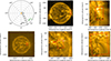 |
Fig. 3. Viewing geometry and multi-scale context in the 171 Å channel. Top left: Relative positions of SDO (near Earth) and STEREO-A in the heliographic Stonyhurst frame at the time of observation. Top middle: Full-disk AIA 171 Å image with the selected limb segment shown in red. Top right: Zoomed AIA view of the limb region containing the two prominences, with arrows marking the prominence footpoints. Bottom left: Corresponding full-disk STEREO-A/EUVI 171 Å image with the projected limb segment. Bottom middle: Intermediate EUVI zoom providing additional spatial context. Bottom right: Tight EUVI zoom of the prominence region, with arrows indicating the same footpoints as in the AIA panel. |
However, the relatively strong signal of prominence 1A in Hα, combined with its faint presence in the AIA 1700 channel, suggests that it is not independent of the surrounding active regions. Because prominence emission is largely governed by the resonant scattering of incident solar radiation (e.g., Heinzel 2015; Jenkins et al. 2023; Heinzel & Gunár 2025), the bright surroundings of prominence 1A mean that it should not be considered quiet.
2.2. Prominence 2
The observations of prominence 2 were made with the Fast Multi-Line Universal Spectrograph (FaMuLUS) camera system. This instrument is an upgrade of the echelle spectrograph around which the telescope was built (Schmidt 1991) and consists of four independent CMOS cameras that can simultaneously observe between approximately 3900 Å and 9000 Å. The cameras cover spectral regions between approximately 4.6 Å and 10.7 Å, respectively. The respective spectral resolving power of the spectrograph extends from approximately  to 431 000. The spectra are critically sampled at approximately 4950 Å. At shorter wavelength, the spectra are undersampled, and at longer wavelength, they are oversampled, with a a pixel size of 4.6 μm and a 4-pixel binning along the dispersion direction.
For the observations we studied, FaMuLUS was configured to cover four spectral windows, that is, G-band at 4307 Å, Cr I at 5782 Å, Hα at 6563 Å, and Ca II at 8542 Å. The respective exposure times were 300 ms, 400 ms, 970 ms, and 970 ms for each slit position. During one scan, which takes just over 6 min, the 216″ long slit scans a dense raster with 334 steps of 0.36″, resulting in slit-reconstructed maps with a size of 216″ × 120″. The data were reduced with the standard FaMuLUS data pipeline.
Prominence 2 was observed on the south-eastern side of the limb at helioprojective Cartesian coordinates (x, y) = (−687″, − 705″) at 08:25 UT on 2025 November 19 for one scan. Unlike prominence 1A, this prominence is in a quiet-Sun region, far enough away from any active region, and can be considered a typical quiescent prominence (e.g., Engvold 2015). Figure 1 shows a triangular shape in the AIA 304 Å channel with a dense, narrow spine in the AIA 171 Å channel. No signal is seen in the AIA 1600 Å image, but an elliptical cavity, resembling the structure simulated and later modeled in Liakh & Keppens (2023) and Pietrow et al. (2024), can be seen in the AIA 211 Å channel. Its appearance in GONG resembles the more typical-looking prominence 1B from the Sol’Ex observations.
Prominence 2 was also observed with Sol’Ex spectroheliograph, and a significantly weaker signal was found compared to prominence 1A (Váradi Nagy 2025), making it impossible to extract a usable spectrum from the 4-centimeter spectroheliograph. This means that prominence 2 is likely more comparable to prominence 1B than the active prominence 1A.
3. Results and discussion
In this section, we discuss the post-reduction methods for both prominences. We then fit the FaMuLUS emission lines and estimate their Doppler-broadening term.
3.1. Sol’Ex observations of prominence 1A
First, a second-order polynomial was fit to the solar limb to quantify its curvature, and each image column was subsequently shifted to produce a flattened limb. The prominence signal was then isolated following Váradi Nagy (2025) by averaging the three spectral pixels centered on the Ti II 4307.9 Å line and subtracting the nearby continuum at 4307 Å, thereby constructing a filtergram that highlights the prominence structure. A contour was used to mark this structure in the spectral cube, and the same contour shifted by 20″ to the left was used as a background reference. The final spectrum was obtained by subtracting these two structures and gauging their intensity relative to that of the quiet Sun. In the left panel of Fig. 2, we show the resulting prominence signal, the fitted contour (red), and a comparative GONG Hα contour (green). In the right panel of the same figure, we show the disk center spectrum in black, the resulting prominence spectrum in red, the Ti II 4307.9 Å average in violet, and the continuum in tan.
The resulting spectra show a relatively clean signal with nine emitting features, two of which are significantly stronger than the rest. Using Moore et al. (1966), we identified the most likely candidates for these lines, although an exact line identification remains difficult. The two strongest lines are attributed to Ti II at 4307.9 Å and 4300.1 Å. In addition, seven weaker emission features are attributed to Ca I, Ti II, Fe II, and Sc II lines. In addition to these nine lines, several features are visible between 4302 Å and 4308 Å in a spectral region with many CH features, but their signal and the spectral resolution of the instrument are both too low to attempt an identification. For this reason, the FaMuLUS window was selected to cover these wavelengths (denoted as a gray box in the right panel in Fig. 2).
3.2. FaMuLUS observations of prominence 2
A similar reduction strategy was used on the FaMuLUS data. First, an observation of a 1951 USAF resolution test chart (defined in MIL-STD-150A) was used to spatially align the spectral windows. Next, a second-order polynomial was fit to a spectrally averaged G-band intensity map of the limb, and each column was shifted to create a straightened limb.
An average was then taken at the Ti II line at 4307.91 Å to isolate the prominence signal from the background (left panel in Fig. 4). The area within this prominence (red contour) was then applied to the G-band, Hα, and Ca II data. The same mask was shifted to the left and right of the prominence and averaged to obtain a background estimate. The difference of these two averages can be found in the right panel of Fig. 4 as a smoothed red profile. The same plot contains a black disk-center profile, where all lines with a significant depth are labeled based on the line list provided by Moore et al. (1966).
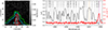 |
Fig. 4. Overview of prominence 2 observations. Left: Prominence 2 imaged in the Ti II line at 4307.91 Å (violet band in the right panel), shown in grayscale as a logarithmic contrast plot with the nearby continuum (tan band in right panel). The green contour indicates the extent of the prominence in an Hα slit-reconstructed line-core intensity map, the cyan contour traces the prominence extent in a Ca II NIR slit-reconstructed line-core intensity map, and the red contour marks the prominence extent of the slit-reconstructed intensity map at 4307.91 Å. Right: Disk-center profile (black) showing the spectral extent of the recording, along with the prominence spectrum (red) after background subtraction. The line identifications are denoted with dashed vertical lines, black for atoms, and gray for CH. |
This wavelength range overlaps with the shaded region in Fig. 2. Within this interval, emission is detected only in the Ti II line at 4307.91 Å and in the Ca I line at 4307.75 Å, while no signal is observed in other spectral features. This implies that the G-band prominence signal is primarily associated with metal lines and not with lines of the CH molecule.
3.3. Diagnostic potential
From the observations of prominence 1A and prominence 2, we found that the emission is dominated by Ca I and Ti II lines, with no discernible signal from the CH molecules. Using the NIST Atomic Spectra Database Lines Data (Kramida et al. 2024), we found that the Ca I line at 4302.55 Å and the Ca I line at 4307.75 Å are both part of the same multiplet and share similar line strengths (Olsen et al. 1959). For the Ti II lines, we found two multiplets (Pickering et al. 2001) that connect the two bright lines and the four dimmer lines in Fig. 2.
The signal from prominence 1A is stronger by approximately two orders of magnitude than that of prominence 2, which might be due to a combination of physical and instrumental effects. Nevertheless, we restricted our quantitative analysis to prominence 2 and used the prominence 1A signal solely for line identification where possible.
Despite their relatively weak signals and blending, the combination of the Ca I line at 4307.75 Å and the Ti II line at 4307.91 Å makes this region an interesting diagnostic for comparisons between ions and neutrals. In particular, as a test of nonthermal motions between ions and neutrals because these lines are observed strictly simultaneously in the same wavelength range.
A difference in these motions was first reported by Landman (1981), who demonstrated that spectral lines formed by ions and neutrals do not necessarily exhibit identical widths, as ions are directly coupled to the magnetic field, whereas neutrals are not. This suggests that neutrals will sink through the magnetic structure of the prominence when not in collisional equilibrium with charged particles, and such an effect was shown by Gilbert et al. (2002, 2007) for helium at the top of prominences. However, more recent work demonstrated that this is not always the case, and neutrals have been reported with nonthermal widths similar to those of ions (e.g., Stellmacher & Wiehr 2015; Wiehr et al. 2019, 2021, 2025).
These works proposed an ionization memory effect, where recently recombined neutrals retain a memory of their prior ionized state, as the time between recombination and emission is much shorter than the collision time needed to erase the ion-induced velocity distribution. We repeated the methods of Wiehr et al. (2025) and applied them to the observations of prominence 2.
The intensities of the prominences were calibrated to the nearby disk-center continuum intensity using the ISPy library. In Fig. 5, the signals of all three windows are shown in background-subtracted intensity units. The total energy of the prominence was calculated by integrating the Hα line profile over the wavelength (gray box in top panel of Fig. 5), yielding the line-integrated specific intensity. This value was placed on an absolute scale using the quiet-Sun continuum from Labs & Neckel (1968). The resulting line-integrated intensity was then compared to the values listed in Gouttebroze et al. (1993), which can in turn be used to infer an approximate temperature for the prominence. However, this estimate is very sensitive to broadening effects induced by Doppler shifts, and because we averaged over a large area (see Fig. 4), we likely integrated over several strands. This places the temperature at either 6000 K or 8000 K.
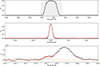 |
Fig. 5. Processed prominence signals in the Hα line, the Ca II line, and the Ca I and Ti II line pair of the G-band, normalized to the local disk-center intensity. For the first row, a sum (gray box) is taken over the non-Gaussian emission profile to obtain the integrated line intensity of the prominence. A Gaussian was fit to the emission of the other two prominences. The best-fit parameters of these Gaussians are given in Table 1. |
Following Wiehr et al. (2025), we took the total broadening as the sum of the thermal and nonthermal terms vobs2 = vth2 + vnth2. The thermal term was defined as vth2 = 2RT/μ, with R the gas constant, T the temperature, and μ the atomic mass. The total broadening was defined as  , with c the speed of light, σ the width of the Gaussian, and λ0 the rest wavelength. Combined, this yields
 (1)
(1)
For Hα, we have a maximum background-subtracted intensity of 6.00 × 10⁻²I/Ic, and an integrated intensity of 5.99 × 10⁻² Å I/Ic, which gives an energy of 1.68 × 10⁵ erg cm−2 ster−1 s−1. In Table 1 we show the line intensities normalized with respect to the local continuum, the fit parameters, and the nonthermal widths resulting from the two assumed temperatures. For 8000 K, we obtained a thermal width that exceeds the total width of Ca I, which suggests that this temperature is too high for this prominence. At 6000 K, we found very similar nonthermal velocities for both ions, but a much lower value for Ca I, suggesting a more classical two-fluid approximation, as suggested by Landman (1981).
Measured prominence line properties, including peak intensity, Gaussian width σ, line width Δλw, and derived nonthermal velocities for assumed temperatures of 6000 K and 8000 K.
Because the signal-to-noise ratio of this emission is low and the blending from the nearby Ti II line is strong, no firm conclusions can be drawn for the Ca I line at 4307.75 Å line. Nevertheless, since most spectral lines examined in previous studies form higher in the atmosphere and correspond to more readily ionized species, it is plausible that the memory effect is less pronounced for weaker (low-forming in the photosphere) neutral lines such as the Ca I line at 4307.75 Å. If this is indeed the case, then such lines might be used together with more classically used prominence lines to accurately gauge the prominence temperature, similarly to how this is done with millimeter observations (Labrosse et al. 2022).
4. Conclusions
We presented spectroscopic observations of two solar prominences in the Fraunhofer G-band observed with an amateur-built Sol’Ex spectroheliopgraph and the FaMuLUS camera system at the VTT echelle spectrograph. In both cases, clear emission was detected from ionized and neutral metal lines (primarily Ti II and Ca I lines), while no signal was measured in the plethora of molecular CH lines that dominate this wavelength window (see Figs. 2 and 4). In this sense, the observed structures are better described as prominences in the G-band than G-band prominences, as the latter would imply structures related to G-band diagnostics based on the CH molecule.
We also demonstrated the value of collaborations with amateur astronomers, who benefit from technological advances, making better telescope optics, filters, and spectrograph more affordable. In addition, amateurs have significant hands-on experience in solar observations, operate in large numbers and in various locations, thus raising the odds of observing of rare events and exceptional features occurring on the Sun.
In these observations, we found no clear evidence of a strong ionization memory signature in the weak neutral line. If confirmed by follow-up observations with larger and more sensitive telescopes, this effect will make these lines a valuable diagnostic for constraining prominence temperatures.
Acknowledgments
AP was supported by grant PI 2102/1-1 from the Deutsche Forschungsgemeinschaft (DFG). MV acknowledges the support from IGSTC-WISER grant (IGSTC-05373). We thank Ralph Smith for his attempts to photometrically observe these prominences with an Altair G-band Solar Filter. Additionally, we thank Aaron Peat and Veronika Jerčić for valuable discussions and comments on the manuscript. We also gratefully acknowledge the Struve Solar Society for fostering a collaborative space between amateur and professional solar observers. The VTT is operated by a German consortium led by the Institute for Solar Physics (KIS) in Freiburg, with the AIP and the Max Planck Institute for Solar System Research (MPS) in Göttingen as partners. This research has made use of the bibliographic services of NASA’s Astrophysics Data System (ADS). DeepL Write was used for assistance with grammar and language polishing.
References
- Bodnárová, M., Utz, D., & Rybák, J. 2014, Sol. Phys., 289, 1543 [CrossRef] [Google Scholar]
- Buil, C., Malherbe, J.-M., & Maksimovic, M. 2023, Photoniques, 120, 36 [Google Scholar]
- Champeau, C. 2026, https://doi.org/10.5281/zenodo.19582043 [Google Scholar]
- Díaz Baso, C., Vissers, G., Calvo, F., et al. 2021, https://doi.org/10.5281/zenodo.5608441 [Google Scholar]
- Engvold, O. 2015, in Solar Prominences, eds. J. C. Vial, & O. Engvold, Astrophys. Space Sci. Lib., 415, 31 [NASA ADS] [Google Scholar]
- Fraunhofer, J. 1817, Ann. Phys., 56, 264 [Google Scholar]
- Gilbert, H. R., Hansteen, V. H., & Holzer, T. E. 2002, ApJ, 577, 464 [NASA ADS] [CrossRef] [Google Scholar]
- Gilbert, H., Kilper, G., & Alexander, D. 2007, ApJ, 671, 978 [Google Scholar]
- Gouttebroze, P., Heinzel, P., & Vial, J. C. 1993, A&AS, 99, 513 [NASA ADS] [Google Scholar]
- Harvey, J. W., Hill, F., Hubbard, R. P., et al. 1996, Science, 272, 1284 [Google Scholar]
- Heinzel, P. 2015, in Solar Prominences, eds. J. C. Vial, & O. Engvold, Astrophys. Space Sci. Lib., 415, 103 [Google Scholar]
- Heinzel, P., & Gunár, S. 2025, Sol. Phys., 300, 167 [Google Scholar]
- Howard, R. A., Moses, J. D., Vourlidas, A., et al. 2008, Space Sci. Rev., 136, 67 [NASA ADS] [CrossRef] [Google Scholar]
- Isobe, H., Kubo, M., Minoshima, T., et al. 2007, PASJ, 59, S807 [Google Scholar]
- Jenkins, J. M., Osborne, C. M. J., & Keppens, R. 2023, A&A, 670, A179 [NASA ADS] [CrossRef] [EDP Sciences] [Google Scholar]
- Johnson, H. L., & Morgan, W. W. 1953, ApJ, 117, 313 [NASA ADS] [CrossRef] [Google Scholar]
- Kamlah, R., Verma, M., Denker, C., et al. 2025, Sol. Phys., 300, 62 [Google Scholar]
- Labrosse, N., Rodger, A. S., Radziszewski, K., et al. 2022, MNRAS, 513, L30 [NASA ADS] [CrossRef] [Google Scholar]
- Labs, D., & Neckel, H. 1968, ZAp, 69, 1 [Google Scholar]
- Landman, D. A. 1981, ApJ, 251, 768 [Google Scholar]
- Langhans, K., & Schmidt, W. 2002, A&A, 382, 312 [NASA ADS] [CrossRef] [EDP Sciences] [Google Scholar]
- Lee, Y. S., Beers, T. C., Sivarani, T., et al. 2008, AJ, 136, 2022 [Google Scholar]
- Lemen, J. R., Title, A. M., Akin, D. J., et al. 2012, Sol. Phys., 275, 17 [Google Scholar]
- Liakh, V., & Keppens, R. 2023, ApJ, 953, L13 [NASA ADS] [CrossRef] [Google Scholar]
- Moore, C. E., Minnaert, M. G. J., & Houtgast, J. 1966, The Solar Spectrum 2935 Å to 8770 Å (Wahington, DC: National Bureau of Standards) [Google Scholar]
- Neckel, H., & Labs, D. 1984, Sol. Phys., 90, 205 [Google Scholar]
- Kramida, A., Yu, R., Reader, J., & NIST ASD Team 2024, NIST Atomic Spectra Database (Ver. 5.12), https://physics.nist.gov/asd, accessed: 2025 December 16 (Gaithersburg, MD: NationalInstitute of Standards and Technology) [Google Scholar]
- Olsen, K. H., Routly, P. M., & King, R. B. 1959, ApJ, 130, 688 [Google Scholar]
- Pesnell, W. D., Thompson, B. J., & Chamberlin, P. C. 2012, Sol. Phys., 275, 3 [Google Scholar]
- Pickering, J. C., Thorne, A. P., & Perez, R. 2001, ApJS, 132, 403 [Google Scholar]
- Pietrow, A. G. M. 2026, Open J. Astrophys., 9, 58273 [Google Scholar]
- Pietrow, A. G. M., Liakh, V., Osborne, C. M. J., Jenkins, J., & Keppens, R. 2024, A&A, 690, L15 [NASA ADS] [CrossRef] [EDP Sciences] [Google Scholar]
- Schmidt, W. 1991, Rev. Mod. Astron., 4, 117 [Google Scholar]
- Schröter, E. H., Soltau, D., & Wiehr, E. 1985, Vistas Astron., 28, 519 [CrossRef] [Google Scholar]
- Shelyag, S., Schüssler, M., Solanki, S. K., Berdyugina, S. V., & Vögler, A. 2004, A&A, 427, 335 [NASA ADS] [CrossRef] [EDP Sciences] [Google Scholar]
- Stellmacher, G., & Wiehr, E. 2015, A&A, 581, A141 [NASA ADS] [CrossRef] [EDP Sciences] [Google Scholar]
- Tandberg-Hanssen, E. 1995, The Nature of Solar Prominences (Dordrecht, The Netherlands: Springer Science+Business Media) [Google Scholar]
- Váradi Nagy, P. 2024, Prominences in G-band - Spectral Imaging, https://www.asztrofoto.hu/galeria_image/1727382235, accessed: 2025 December 13, image posted on Asztrofotó.hu [Google Scholar]
- Váradi Nagy, P. 2025, Prominences in the G-band and Beyond, https://csillagtura.ro/prominences-in-the-g-band-and-beyond, accessed: 2025 December 13 [Google Scholar]
- Váradi Nagy, P., & Pietrow, A. G. M. 2025, RNAAS, 9, 188 [Google Scholar]
- von der Lühe, O. 1998, New Astron. Rev., 42, 493 [Google Scholar]
- Wiehr, E., Stellmacher, G., & Bianda, M. 2019, ApJ, 873, 125 [Google Scholar]
- Wiehr, E., Stellmacher, G., Balthasar, H., & Bianda, M. 2021, ApJ, 920, 47 [NASA ADS] [CrossRef] [Google Scholar]
- Wiehr, E., Balthasar, H., Stellmacher, G., & Bianda, M. 2025, A&A, 696, A209 [NASA ADS] [CrossRef] [EDP Sciences] [Google Scholar]
- Wuelser, J. P., Lemen, J. R., Tarbell, T. D., et al. 2004, in Telescopes and Instrumentation for Solar Astrophysics, eds. S. Fineschi, & M. A. Gummin, Proc. SPIE, 5171, 111 [NASA ADS] [CrossRef] [Google Scholar]
All Tables
Measured prominence line properties, including peak intensity, Gaussian width σ, line width Δλw, and derived nonthermal velocities for assumed temperatures of 6000 K and 8000 K.
All Figures
|
Fig. 1. GONG and SDO/AIA observations of two prominences in the Hα, 1600 Å, 304 Å, 171 Å, and 211 Å channels, sampling plasma from the upper chromosphere and transition region to the low corona. The top row shows prominence 1A (observed at 08:47 UT on the 9th of Oktober 2025), located adjacent to an active region, while the bottom row shows prominence 2 (observed at 08:47 on the 11th of November 2025) in a quieter coronal environment. The white arrows indicate the prominence structures in each channel. The red boxes indicate the FOV of the cuts made in the figures below. |
| In the text | |
|
Fig. 2. Overview of prominence 1A observations. Left: Prominence 1A imaged in the Ti II 4307.9 Å line (violet line in the right plot) shown in grayscale after the nearby continuum was subtracted (tan line in the right plot). The green contour represents the extent of the prominence in a GONG Hα filtergram. Right: Disk center profile (black) showing the spectral extent of the recording, along with the prominence spectrum (red) after normalization to the disk center continuum intensity. The nine brightest emission lines are marked with dashed vertical lines. The gray shaded region corresponds to the spectral FaMuLUS window. |
| In the text | |
|
Fig. 3. Viewing geometry and multi-scale context in the 171 Å channel. Top left: Relative positions of SDO (near Earth) and STEREO-A in the heliographic Stonyhurst frame at the time of observation. Top middle: Full-disk AIA 171 Å image with the selected limb segment shown in red. Top right: Zoomed AIA view of the limb region containing the two prominences, with arrows marking the prominence footpoints. Bottom left: Corresponding full-disk STEREO-A/EUVI 171 Å image with the projected limb segment. Bottom middle: Intermediate EUVI zoom providing additional spatial context. Bottom right: Tight EUVI zoom of the prominence region, with arrows indicating the same footpoints as in the AIA panel. |
| In the text | |
|
Fig. 4. Overview of prominence 2 observations. Left: Prominence 2 imaged in the Ti II line at 4307.91 Å (violet band in the right panel), shown in grayscale as a logarithmic contrast plot with the nearby continuum (tan band in right panel). The green contour indicates the extent of the prominence in an Hα slit-reconstructed line-core intensity map, the cyan contour traces the prominence extent in a Ca II NIR slit-reconstructed line-core intensity map, and the red contour marks the prominence extent of the slit-reconstructed intensity map at 4307.91 Å. Right: Disk-center profile (black) showing the spectral extent of the recording, along with the prominence spectrum (red) after background subtraction. The line identifications are denoted with dashed vertical lines, black for atoms, and gray for CH. |
| In the text | |
|
Fig. 5. Processed prominence signals in the Hα line, the Ca II line, and the Ca I and Ti II line pair of the G-band, normalized to the local disk-center intensity. For the first row, a sum (gray box) is taken over the non-Gaussian emission profile to obtain the integrated line intensity of the prominence. A Gaussian was fit to the emission of the other two prominences. The best-fit parameters of these Gaussians are given in Table 1. |
| In the text | |
Current usage metrics show cumulative count of Article Views (full-text article views including HTML views, PDF and ePub downloads, according to the available data) and Abstracts Views on Vision4Press platform.
Data correspond to usage on the plateform after 2015. The current usage metrics is available 48-96 hours after online publication and is updated daily on week days.
Initial download of the metrics may take a while.