| Issue |
A&A
Volume 710, June 2026
|
|
|---|---|---|
| Article Number | A25 | |
| Number of page(s) | 24 | |
| Section | Interstellar and circumstellar matter | |
| DOI | https://doi.org/10.1051/0004-6361/202554989 | |
| Published online | 28 May 2026 | |
Massive star formation at the Galactic crossroads: Insights from G358.69+0.03 in the Galactic center
1
Max Planck Institute for Radioastronomy (MPIfR),
Auf dem Hügel 69,
53121
Bonn,
Germany
2
Department of Astronomy & Astrophysics, Tata Institute of Fundamental Research,
Homi Bhabha Road,
Mumbai
400005,
India
3
MIT Haystack Observatory,
99 Millstone Road,
Westford,
MA
01827,
USA
4
Deutsches Zentrum für Astrophysik,
Postplatz 1,
02826
Görlitz,
Germany
5
National Radio Astronomy Observatory,
PO Box O, 1003 Lopezville Road,
Socorro,
NM
87801,
USA
6
Purple Mountain Observatory, and Key Laboratory of Radio Astronomy, Chinese Academy of Sciences,
10 Yuanhua Road,
Nanjing
210023,
PR China
★ Corresponding author: This email address is being protected from spambots. You need JavaScript enabled to view it.
Received:
1
April
2025
Accepted:
30
March
2026
Abstract
We investigated the high-mass star formation activity in a subregion of the Sagittarius E star-forming complex, centered at (l, b) = (358.69°, 0.03°), where infrared and radio sources trace a prominent U-shaped structure that has not been identified in previous studies. We used radio continuum data from the Global View on Star Formation (GLOSTAR) survey, which is a wide-band radio (4–8 GHz) survey of the Milky Way that combines data from the Karl G. Jansky Very Large Array and the Effelsberg 100 m telescope. Using BLOBCAT source extraction software, we identified 49 compact radio sources. Based on multiwavelength associations and spectral index estimates, we identified GLOSTAR counterparts to 27 previously confirmed H II regions, detected radio emission from 3 WISE “radio-quiet” candidates, and report 5 new H II region candidates. The derived physical properties indicate that most are relatively evolved H II regions. We find around 50 cold dust clumps, predominantly toward the south and southeast. Mid-infrared flux-ratio maps ([4.5]/[3.6]) show localized shock enhancements along the arc and adjacent clumps, and 15 clumps exhibit SiO emission with broad components indicative of shocks. Together with CO data, the SiO velocity components delineate a continuous (>100 km s−1) velocity bridge that links the far dust-lane inflow to the central molecular zone (CMZ) stream. The largest concentration of clumps and compact H II regions lies at this interface. These combined diagnostics favor a scenario in which bar-driven cloud–cloud collision at the far dust-lane–CMZ interface compressed the gas and triggered the observed high-mass star formation.
Key words: stars: formation / HII regions / ISM: molecules / galaxy: center / galaxy: evolution
Member of the International Max Planck Research School (IMPRS) for Astronomy and Astrophysics at the Universities of Bonn and Cologne.
Deceased.
© The Authors 2026
 Open Access article, published by EDP Sciences, under the terms of the Creative Commons Attribution License (https://creativecommons.org/licenses/by/4.0), which permits unrestricted use, distribution, and reproduction in any medium, provided the original work is properly cited.
This article is published in open access under the Subscribe to Open model.
Open Access funding provided by Max Planck Society.
1 Introduction
Massive star formation and its radiative and mechanical feedback are critical drivers of galactic evolution. In this context, the nuclear regions of galaxies are particularly important, as they often exhibit more extreme physical, chemical, and kinematic conditions than the galactic disks. However, studying extragalactic nuclei poses significant observational challenges due to high interstellar extinction and the need for subarcsecond angular resolution to overcome severe source crowding. The Milky Way’s Galactic center (GC) offers a unique local laboratory for investigating massive star formation under such extreme conditions (Shetty et al. 2012; Longmore et al. 2013; Ginsburg et al. 2016; Barnes et al. 2017; Henshaw et al. 2016, 2023, and references therein). By exploring the physical processes and chemistry of the Milky Way’s nucleus, we not only gain insights into its formation and evolution but also establish a critical template for interpreting the central regions of nearby galaxies.
The central molecular zone (CMZ), which is the innermost few hundred parsecs of the Milky Way, holds approximately 2–6 × 10⁷ M⊙ of molecular material, accounting for ≲10% of the total molecular gas and ~80% of the dense gas within the Milky Way (Ferrière et al. 2007; Molinari et al. 2014; Roman-Duval et al. 2016; Battersby et al. 2025, etc.). It hosts plentiful energetic phenomena, most importantly the ongoing and past massive star formation activity in complexes such as Sgr B2 and Sgr C. The CMZ roughly spans the Galactic longitude range of −1° ≲ l ≲ 1.7° (Henshaw et al. 2023), with mass inflow into the region facilitated by two dust lanes along the Galactic bar. The near-side dust lane, called the connecting arm, is situated at l > 0°, and the far-side dust lane merges with the CMZ at l < 0° (Marshall et al. 2008; Sormani & Barnes 2019; Henshaw et al. 2023). Due to the energetic conditions, the CMZ is expected to have a high star formation rate (SFR).
Yusef-Zadeh et al. (2009) studied the central 400 × 50 pc region of the GC and observed an asymmetry in the distribution of the candidate young stellar objects (YSOs), with a higher concentration toward the negative Galactic longitudes. They estimated the SFR based on the identification of Stage I YSO candidates to be about 0.14 M⊙ yr−1, which is much higher than the SFR estimates of the CMZ in literature of, for example, ~0.08 M⊙ yr−1 (Hatchfield et al. 2024) and ~0.068 M⊙ yr−1 (Nguyen et al. 2021). The asymmetry of YSOs has been a matter of scientific controversy, with many studies providing conflicting conclusions. For example, Koepferl et al. (2015) studied the sample of YSOs from Yusef-Zadeh et al. (2009) using radiative transfer models and showed that embedded main sequence stars can masquerade as YSOs. This misclassification could lead to incorrect conclusions regarding the distribution of YSOs and, consequently, affect the inferred SFR of the CMZ.
Anderson et al. (2020) further investigated massive star formation activity along the negative Galactic longitudes, in particular in the star-forming complex Sagittarius E (Sgr E; 358.3° < l < 359.3°; |b|<0.2°; Liszt 1992; Gray et al. 1993; Gray 1994; Cram et al. 1996). Sgr E is located at a projected distance of ~220 pc from the GC, at the intersection of the CMZ and the far dust lane. Using 1.28 GHz MeerKAT GC data and radio recombination line (RRL) observations from the Green Bank Telescope, they found 19 H II regions and 43 H II region candidates embedded in a molecular cloud of mass 3 × 10⁵ M⊙, highlighting the region as a hot spot of high-mass star formation in the GC. They propose that SgrE formed upstream in the far dust lane a few million years ago, and would likely overshoot the CMZ and crash into the near dust lane.
Upon further investigation, we noticed a striking arc-like or U-shaped distribution of the compact H II regions in a subregion of the SgrE complex (see Fig. 1). The region also shows relatively strong radio and infrared emission along a similar U-shaped morphology. In the present study, we conducted an extensive analysis of the star formation activity within this subregion of the SgrE complex, hereafter referred to as G358.69+0.03 (see Fig. 2). It has a radius of approximately 0.26°, which corresponds to about 37.48 pc at the GC distance of 8.2 kpc (GRAVITY Collaboration 2019), and is centered at Galactic coordinates l = 358.69°, b = 0.03°. We further refined the population of H II regions, tracers of massive star formation activity, using observations from the Karl G. Jansky Very Large Array (VLA) D configuration at a higher frequency of 5.8 GHz. Additionally, we examined the distribution of cold dust clumps and the signature of shocks, and explored the possibility of a triggered star formation scenario to explain the region’s morphology.
Section 2 gives a summary of the data used in this study. Section 3 describes the source extraction procedures and the multiwavelength analysis performed to identify the candidate H II (cH II) regions. Section 4 provides details on the properties of the target region and the distribution of cold dust clumps and shock signatures across G358.69+0.03. Section 5 discusses the triggered star formation scenario invoked to explain the morphology of our target region. We present our conclusions in Sect. 6.
 |
Fig. 1 Left: three-color infrared view of the Galactic plane on the negative longitude side, with MIPSGAL 24 μm emission in red, GLIMPSE 8 μm in green, and GLIMPSE 4.5 μm in blue. The golden box shows the SgrE star-forming complex (358.3°<l<359.3°, |b| < 0.2°; Anderson et al. 2020). Right: 1.28 GHz MeerKAT image of the target region (Heywood et al. 2022). The dashed partial circles in both panels highlight the arc-like or U-shaped morphology of G358.69+0.03. |
2 Data
2.1 Radio continuum observations
Over the past few decades, there have been a large number of Galactic plane surveys of the Milky Way, observing both spectral-line and continuum emission covering the entire wavelength range from the near-infrared (NIR) to the radio (Becker et al. 1994; Lucas et al. 2008; Carey et al. 2009; Schuller et al. 2009; Aguirre et al. 2011; Molinari et al. 2016; Beuther et al. 2016, etc.). To study high-mass star formation activity at the negative Galactic longitudes of the Milky Way, we used data from the Global View on Star Formation (GLOSTAR1) survey (Medina et al. 2019; Brunthaler et al. 2021).
The GLOSTAR survey is the most sensitive radio survey (~60–150 μJy beam−1) of the Galactic plane at the C-band of 4–8 GHz. The observations were conducted using the upgraded VLA of the National Radio Astronomy Observatory (NRAO) and the Effelsberg 100 m telescope with increased frequency coverage and unprecedented sensitivity. The main objective of the survey is to study massive star formation activity in the Galactic mid-plane of the Milky Way. The survey simultaneously observes radio continuum in full polarization and spectral line emission such as the 6.7 GHz methanol maser line, 4.8 GHz formaldehyde line and seven RRLs covering the velocity range of −150 km s−1 to +150 km s−1 (Brunthaler et al. 2021). In the continuum mode, the survey observes different evolutionary stages of the tell-tale tracers of high-mass star formation, namely hypercompact, ultracompact, and compact H II regions (Medina et al. 2019; Nguyen et al. 2021; Dzib et al. 2023; Yang et al. 2023; Khan et al. 2024; Medina et al. 2024).
The GC (|l| < 2°; |b| < 1°) was observed using the C-band receivers (4–8 GHz) of the VLA in the DnC configuration, i.e., the northern arm of the VLA was in the C configuration and the other two arms were in the D configuration, providing an angular resolution of 18″. This configuration gives a more circular beam for low-declination sources. The correlator setup consists of two 1 GHz sub-bands, centered at 4.7 and 6.9 GHz; they have primary beams with full widths at half maximum (FWHMs) of ~9′ and ~6′, respectively (Medina et al. 2019; Brunthaler et al. 2021). Each sub-band consisted of 8 spectral windows of 128 MHz each, which are further divided into 64 channels of 2 MHz each. The GC observations were conducted in September-October 2014 and January 2016. The data were then calibrated using a modified pipeline created using the Obit software package (Cotton 2008), which is explained in more detail in Medina et al. (2019). The resultant VLA-D integrated intensity radio continuum map with an effective frequency of 5.8 GHz and a pixel size of 2.5″ is shown in the left panel of Fig. 2.
The VLA data were complemented with low-resolution ~150″ images from single-dish observations of the Effelsberg 100 m radio telescope. This was done to provide the zero spacings for the D configuration data to recover the extended emission. The image combination process and the caveats are discussed in detail in Dokara et al. (2023). The single dish Effelsberg observations were carried out in July 2020 and April 2021. The resultant integrated intensity VLA-D+Effelsberg map of the target region is shown in the right panel of Fig. 2.
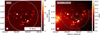 |
Fig. 2 Left: GLOSTAR D configuration radio continuum averaged intensity map at 5.8 GHz with an angular resolution of ~18″. The dashed white circle marks the target region. Right: GLOSTAR combination image (VLA-D+Effelsberg). The dashed cyan partial circles highlight the arc-like or U-shaped morphology of G358.69+0.03. The beam sizes are shown in the lower-left corner of each panel. |
2.2 APEX nFLASH follow-up
To study SiO emission from a cluster of dust clumps located toward the south of the target region, we selected 17 sources from the APEX Telescope Large Area Survey of the Galaxy (ATLASGAL) Compact Source Catalogue (CSC; Urquhart et al. 2014). We carried out the standard position switch observations using the Atacama Pathfinder Experiment (APEX) 12 m telescope (Güsten et al. 2006) in March 2023 (ID: M-0111.F-9523C-2023). The total observing time was 11.8 hours. We used the nFLASH230 receiver as the frontend instrument tuned at 230.79 GHz in the upper sideband (USB) and the fast Fourier transform spectrometer (FFTS1) as the backend instrument. The spectral resolution is 0.25 km s−1, and the APEX/nFLASH230 beam FWHM is ~26.2″2. The receiver covers a total of 32 GHz IF instantaneous bandwidth, including both sidebands and polarizations. The setup covers the SiO (5–4) transition with a rest frequency of 217104.984 MHz, which is considered a good shock tracer (Schilke et al. 1997).
The antenna temperatures (![Mathematical equation: $\[T_{A}^{*}\]$](/articles/aa/full_html/2026/06/aa54989-25/aa54989-25-eq1.png) ) were converted to the main beam brightness temperature (TMB) scale using a beam efficiency factor of 0.83. The data reduction was performed using the GILDAS3 software (Pety 2005).
) were converted to the main beam brightness temperature (TMB) scale using a beam efficiency factor of 0.83. The data reduction was performed using the GILDAS3 software (Pety 2005).
2.3 Archival data
To carry out a comprehensive multiwavelength analysis, we used archival data from complementary multiwavelength surveys.
2.3.1 Spitzer Space Telescope
We used the images from the Galactic Legacy Infrared Mid–Plane Survey Extraordinaire (GLIMPSE), a legacy program observed using the Infrared Array Camera (IRAC) on board the Spitzer Space Telescope (Benjamin et al. 2003; Churchwell et al. 2005) to study the mid-infrared (MIR) morphology of the target region. It covers the wavelength range from 3.6 μm to 8.0 μm with an angular resolution of ~2″. We also used the 24 μm MIR image with an angular resolution of 6″ covered using the Multiband Infrared Photometer for Spitzer (MIPSGAL) on board the Spitzer Space Telescope (Carey et al. 2009). We also utilized the GLIMPSE II Epoch 1 Catalog (Glimpse Team 2020) and the MIPSGAL 24 μm Catalog (Gutermuth & Heyer 2020) obtained from the NASA/IPAC Infrared Science Archive (IRSA4).
2.3.2 WISE
We utilized the Wide-field Infrared Survey Explorer (WISE) maps at wavelengths of 3.4, 4.6, 12, and 22 μm, having angular resolutions of 6.1″, 6.4″, 6.5″, and 12.0″, respectively (Wright et al. 2010), to study the MIR signature of the target region. We also utilized the WISE All-sky Source Catalog (WISE Team 2020) accessed from IRSA.
2.3.3 Herschel Hi-GAL survey
To investigate the structure associated with the cold and diffuse interstellar dust in the target region, we used the images and photometric compact source catalogs from the Herschel infrared Galactic Plane Survey (Hi-GAL), which observes the inner Galactic plane (68° ≳ l ≳ −70°, |b| ≤ 1°) of the Milky Way at the far-infrared (FIR) wavelengths of 70, 160, 250, 350, and 500 μm using Photodetector Array Camera and Spectrometer (PACS) for the first two and Spectral and Photometric Imaging Receiver (SPIRE) for the last three (Molinari et al. 2016). The angular resolutions are 6″, 12″, 18″, 24″, and 35″, respectively. We also used the 360° CSC (Elia et al. 2021) to study the properties of Hi-GAL clumps.
2.3.4 APEX ATLASGAL survey
We used the images from ATLASGAL taken using the Large APEX Bolometer Camera (LABOCA) at the sub-millimeter wavelength of 870 μm with an angular resolution of 19.2″ (Schuller et al. 2009). The primary goal is to study the earliest embedded stages of massive star formation activity (preand proto-stellar clumps) using the optically thin, thermal emission from dust at submillimeter wavelengths. We also used the ATLASGAL CSC (Urquhart et al. 2014) to study the distribution of cold gas clumps.
2.3.5 CHIMPS2
To explore the large-scale dynamics of the G358.69+0.03 region, we used 12CO(J = 3–2) data from the CO Heterodyne Inner Milky Way Plane Survey 2 (CHIMPS2; Eden et al. 2020), obtained with the James Clerk Maxwell Telescope (JCMT). The spatial resolution, spectral resolution, and root mean square (rms) noise are 15″, 1.0 km s−1, and 0.8 K, respectively. The details of the observations and data reduction are provided in Eden et al. (2020), and the reduced data are available for download from the Canadian Advanced Network for Astronomical Research (CANFAR) archive5.
3 Radio emission and H II region population in G358.69+0.03
A multiwavelength view of G358.69+0.03 is presented in Fig. 1. The infrared three-color composite maps reveal several compact sources embedded within diffuse 8 μm emission, spanning a region of ~30 arcminutes. To characterize the nature of these compact sources and the associated diffuse emission, we analyzed 5.8 GHz data from the GLOSTAR VLA-D configuration and the VLA+Effelsberg observations, shown in Fig. 2. The VLA image reveals numerous compact sources arranged in an arc-like or U-shaped distribution, accompanied by faint extended emission. The VLA+Effelsberg image recovers the extended emission more effectively, highlighting a shell-like structure with compact sources distributed around its periphery. To investigate the population of these compact radio sources, we compiled a catalog, which is detailed in the following subsections.
3.1 Source extraction
We focused on compact H II regions and other emission sources of diameter greater than ~0.7 pc, which can be traced well with GLOSTAR VLA-D configuration images at a distance of 8.2 kpc. The source extraction was performed using this VLA-D configuration image, following the procedures described by Medina et al. (2019) and Dzib et al. (2023).
We used BLOBCAT6, a Python based source extraction software that uses the flood fill algorithm to detect and catalog “blobs” or island of pixels representing sources in 2D astronomical images (FITS files; Hales et al. 2012). The software handles both Gaussian and non-Gaussian sources and produces an output catalog listing the properties of the extracted blobs. BLOBCAT requires two input FITS images and some input arguments to perform the source extraction. The first is the integrated intensity map, i.e., the VLA-D configuration image with an effective frequency of ν ≈ 5.8 GHz and a spatial resolution of 18″. The second is the background rms noise image, which we created using the SExtractor7 tool (Bertin & Arnouts 1996) from the Graphical Astronomy and Image Analysis (GAIA) tool package. SExtractor estimates the noise level at each pixel by extracting the pixel values within a local mesh of user-specified size, and iteratively clipping the extreme values until convergence is reached at a chosen σ value about the median (Hales et al. 2012). Following Medina et al. (2019), we used a detection threshold of 5σ, a minimum size of 5 pixels, and mesh size of 80 × 80 pixels2 to create the noise map, which represents the position-dependent noise excluding most of the real emission from the sources. The rms noise toward the target region was estimated using the Common Astronomy Software Applications package (CASA; McMullin et al. 2007; CASA Team 2022), as σrms ≈ 356 μJy beam−1.
BLOBCAT creates a signal-to-noise ratio (S/N) map by taking pixel-by-pixel ratio of the input integrated intensity and noise maps and extracts blobs using the additional user-specified arguments. Purcell et al. (2013) noted that in their radio continuum images of the Galactic plane observed at 5 GHz using the Coordinated Radio and Infrared Survey for High-Mass Star Formation (CORNISH; Hoare et al. 2012), a majority of radio detections with an S/N of below 4.5 were spurious sources. Hence, we used a S/N threshold for detecting the blob of Td = 5 (dSNR). The minimum accepted blob size in pixels is taken as, minpix = 20, which is the number of expected pixels of size 2.5″ covering 50% of the beam area of size (circular beam of diameter) 18″. We specified a cutoff S/N threshold for flooding of Tf = 3 (fSNR). We tried a number of threshold limits and chose this value based on the visual inspection and comparison with other wavelength images such that BLOBCAT does not misidentify distinct radio sources in crowded fields as one single source. However, in two specific regions – G358.51+0.05 and G358.69–0.08, with sizes of 288″ and 180″, respectively – multiple distinct sources were incorrectly identified as one. So, we ran BLOBCAT separately on these regions with higher cutoff S/N thresholds of 4.6 and 7.6, respectively (see Fig. A.1, for example). A total of 49 sources were extracted, each with a flux above five times the local noise and a size greater than half the beam size. Finally, we performed an individual visual inspection of all these sources and did not find any obvious image artifacts, such as sidelobes from very bright sources. The most reliable sources have peak flux values above 7 σnoise. We have a total of 39 such sources as well as 10 sources with peak fluxes between 5 and 7 times the local noise. Figure B.1 shows all the BLOBCAT-extracted sources toward our target region.
3.2 Multiwavelength associations
To better understand the nature of these 49 radio sources, we searched for their counterparts at other wavelengths. We used a number of infrared surveys that cover the Galactic plane, including the ATLASGAL submillimeter survey (Schuller et al. 2009) and the Multi-Array Galactic Plane Imaging Survey (MAGPIS) radio survey (White et al. 2005); the full list is provided in Sect. 2.3. The catalogs were selected such that their spatial resolutions and/or wavelengths are comparable with those of the GLOSTAR survey. Our main focus is on identifying the cH II regions, which are the most unambiguous tracers of massive star formation activity (Anderson et al. 2014). H II regions are the brightest objects in the Galactic plane at infrared and radio wavelengths (Anderson et al. 2014). They also have characteristic 8 μm emission shells that trace the warm polycyclic aromatic hydrocarbons (PAHs), surrounding emission from the warm dust traced either by 24 μm or radio emission (Simpson et al. 2012). At MIR wavelengths, H II regions also show a characteristic morphology of ~20 μm emission coincident with radio emission tracing the ionized gas, which is surrounded by ~10 μm emission (Anderson et al. 2014, and references therein). The FIR and submillimeter emission associated with cold dense gas and dust can provide evidence of molecular clumps with embedded H II regions (Urquhart et al. 2013). H II regions can show weak signature in the NIR during the deeply embedded stage in the molecular clouds (Yang et al. 2021).
The NIR counterparts were identified using the Two Micron All Sky Survey (2MASS) All-Sky Point Source Catalog (PSC; Skrutskie et al. 2006; Cutri et al. 2003). Within a 4″ search radius, we found 31 cross-matches. Furthermore, we performed a visual inspection to identify multiwavelength counterparts for the BLOBCAT-extracted radio sources across various images from 3.6 μm (MIR) to 870 μm (submillimeter), as well as the radio 1.28 GHz MeerKAT GC image (Heywood et al. 2022). Table B.1 marks the counterparts found for each of the 49 extracted sources across different infrared and radio wavelengths. Additionally, we searched for counterparts in various catalogs listed in detail in Table B.2, which also includes the respective angular resolution and the search radius used to identify potential cross-matches. Notably, some sources had potential matches within the specified search radius but lacked a clear visual signature in the respective maps. These sources are marked with the superscript “c” in Table B.1.
All the BLOBCAT-extracted radio sources have a counterpart in at least one other published radio or infrared catalog, which eliminates the possibility of false detection. We found the most cross-matches in the MIR WISE All-Sky Source Catalog and the least in the ATLASGAL dust continuum and Hi-GAL infrared catalogs. All sources except G358.747–0.154, G358.622+0.093, G358.557+0.243, G358.633+0.240, and G358.688+0.182 have a counterpart in the MeerKAT GC image.
3.3 Spectral index
The spectral index, α (Sν ∝ να, where Sν is the flux density at the observed frequency, ν) helps distinguish between thermal and nonthermal radio sources. H II regions emit thermal bremsstrahlung radiation and usually have spectral indices of around −0.1 (optically thin) and 2 (optically thick) at high and low frequencies, respectively.
The GLOSTAR-VLA image products consist of nine sub-images in the 4–8 GHz frequency range, which we used to estimate the in-band spectral index. Following the procedure explained by Medina et al. (2024), we estimated the spectral indices of compact sources, defined as those with a ratio of integrated to peak flux density (Y-factor) of ≤2, and further imposed S/N > 10 to ensure reliable detection across most sub-images. We extracted the peak flux density and the uncertainty of each source in eight frequency bins, excluding the sub-band with high noise. We then performed least squares fitting using the scipy function curve_fit to the linear equation, log Sν = α × log ν + c.
We estimated spectral indices for 18 of the 49 extracted sources, 7 of which have α ≥ −0.1 within the uncertainty limits. The more reliable estimates of spectral indices are limited to the nine most compact sources with Y-factor ≤1.2. Of these nine sources, five sources have α ≥ −0.1, pointing toward thermal emission.
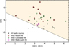 |
Fig. 3 MIR colors for the 37 sources (black crosses) associated with a WISE counterpart out of the total 49 radio sources found toward G358.69+0.03 in this work. The maroon, green, and magenta circles represent the known, candidate, and radio-quiet H II regions, respectively, from the WISE Galactic H II Regions Catalog V2.3 (Anderson et al. 2014). The region above the dashed black line represents the parameter space where all the H II regions and the majority of PNe are present, as identified by Medina et al. (2019). |
3.4 Mid-infrared colors
To further aid to the identification of cH II regions, we examined the MIR colors of our extracted sources using the classification scheme followed by Medina et al. (2019). They generated a MIR color–magnitude diagram of the radio sources in the pilot region of the GLOSTAR survey (28° < l < 36°, |b| < 1°). They classified 231 continuum sources out of the total 1575 discrete radio sources as H II region candidates. They examined the MIR colors of the cataloged H II regions and planetary nebulae (PNe) from their study and from literature (Purcell et al. 2013) and found a good agreement between the datasets. Dust embedded objects, such as H II regions and PNe, exhibit redder MIR colors and occupy a distinct region of the color–magnitude diagram compared to contaminants such as radio stars and extragalactic background sources. Based on that, they proposed a criterion to identify new H II region candidates and defined an area of parameter space using their color–magnitude plot where all of the H II regions and a vast majority of the PNe are located, which is given by
![Mathematical equation: $\[\text { [12]Mag. }<1.74 \times([12]-[22])+2.\]$](/articles/aa/full_html/2026/06/aa54989-25/aa54989-25-eq2.png) (1)
(1)
We identified WISE counterparts using the WISE All-Sky Source Catalog (WISE Team 2020) and found cross-matches for 41 out of the total 49 radio sources within a 10″ search radius. Among these sources, 37 sources have reliable fluxes in all four WISE bands (3.4, 4.6, 12, and 22 μm), and their distribution in the color–magnitude diagram is shown in Fig. 3. Of these 37 sources, 33 lie within the parameter space proposed to be occupied by all the H II regions and a majority of PNe. Among these 33 sources, 12 correspond to known H II regions and 11 are listed as cH II regions in the WISE Galactic H II Regions Catalog V2.3 (hereafter the “WISE H II catalog”; Anderson et al. 2014). Two additional sources are listed in the catalog as radio-quiet H II regions. The remaining 12 sources do not have a counterpart in the WISE H II catalog. We discuss the nature of these sources based on their detailed infrared and radio characteristics in Sect. 3.5.
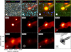 |
Fig. 4 Multiwavelength view of the known H II region, G358.632+0.063. First row (from left to right): Color composite images from 2MASS (Skrutskie et al. 2006), GLIMPSE, WISE, and Spitzer. The red, green, and blue colors are shown in each panel. Middle and bottom rows (from left to right and top to bottom): MIPSGAL 24 μm, Hi-GAL 70 μm, Hi-GAL 160 μm, Hi-GAL 250 μm, Hi-GAL 350 μm, Hi-GAL 500 μm, ATLASGAL 870 μm, and 5.8 GHz GLOSTAR VLA-D images of the H II region. The blue circles in the center of each panel show the peak position of radio emission. The FWHM beams of 2MASS (0.8″), GLIMPSE (2″), WISE (6″ at 12 μm), Spitzer (6″ at 24 μm), MIPSGAL (6″ at 24 μm), Hi-GAL (6″, 12″, 18″, 24″, and 35″ at 70, 160, 250, 350, and 500 μm, respectively), and ATLASGAL (19″) are indicated by the black and white circles with hatched lines shown in the lower-left corner of each panel. |
3.5 Classification of H II regions
Based on our analysis, we cataloged radio sources as H II regions using multiple criteria such as the multiwavelength associations (MIR, FIR, and submillimeter), spectral index estimates, and the MIR color–magnitude diagram. We also looked for known, candidate and radio-quiet H II regions toward G358.69+0.03 using the WISE H II catalog. Among our 49 radio sources, we found 16 known and 11 cH II region cross-matches from the WISE H II catalog, which were classified as H II regions in our work provided they had multiwavelength counterparts. Figure 4 shows an example multiwavelength view for one such known H II region, namely G358.632+0.063. We also found three sources, namely G358.505+0.108, G358.747–0.154, and G358.905+0.029, that had cross-matches with radio-quiet H II regions from the WISE H II catalog, which we then classified as cH II regions. The cross-matches with the WISE H II catalog are shown in Fig. B.2.
The remaining 19 sources were analyzed individually; among them, we identified 5 as new cH II. Table B.3 provides the detailed classification scheme used for their identification. All five new cH II regions occupy the same parameter space in MIR color–magnitude diagram where all the H II regions are located. Three of these sources, namely G358.612+0.178, G358.789–0.020, and G358.822+0.000, have α ≥ −0.1 and at least 24 and 70 μm emission associated with them. Another source, G358.559–0.061, displays cold dust signature and is present at the edge of a radio-quiet H II region. Source G358.758+0.203 has compact emission at 8,24 and 70 μm, with a negative spectral index of α = −0.34 ± 0.15. Although H II regions are known to emit thermal bremsstrahlung radiation (Sect. 3.3), a number of observational studies have revealed the existence of H II regions with a mixture of thermal and nonthermal radiation, with steep negative spectral indices, (e.g., Veena et al. 2016; Nandakumar et al. 2016; Meng et al. 2019; Yang et al. 2023). Using their model of thermal particle acceleration, Padovani et al. (2019) show that shocked H II regions can exhibit nonthermal emission, which might be due to synchrotron radiation from locally accelerated electrons braked in a magnetic field. Our region of interest is present at highly shocked and turbulent location, at the intersection of the CMZ and the far dust lane. The shocked gas is likely to give rise to the nonthermal emission in the target region. We discuss the presence of shock signatures in Sects. 4.3 and 4.4.
The other 14 radio sources that are not classified as H II regions or cH II regions are listed in Table B.4, along with their physical properties obtained from the BLOBCAT software. A few of these sources, namely G358.917+0.072, G358.696+0.263, G358.592+0.046, G358.849+0.161, G358.710+0.136, and G358.631–0.122, have bright and compact radio emission but do not have counterparts at wavelengths from the MIR to the submillimeter. They are also seen as point sources at NIR wavelengths and are likely to be extragalactic candidates (cEGs; Lucas et al. 2008; Hoare et al. 2012). The remaining eight sources have no emission at the submillimeter wavelengths. In the FIR regime, they have no emission from 160 to 500 μm, and a very weak emission at 70 μm. Of these, four, namely G358.823–0.118, G358.533–0.100, G358.633+0.240, and G358.688+0.182 are seen as isolated point sources showing red emission in the NIR and MIR three color composite image. These are classified as candidate planetary nebulae (cPNe; Anderson et al. 2012; Dzib et al. 2023). The nature of the other four sources, two of which have extended radio emission, remains unclear and are hence classified as unidentified radio sources (Rad). Figure 5 illustrates the various types of radio sources toward G358.69+0.03, described above.
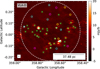 |
Fig. 5 Classification of radio sources toward G358.69+0.03. The green crosses show the HII regions identified in this work. The cyan, magenta, and yellow circles mark the positions of cEGs, cPNe, and the unidentified radio (Rad) sources, respectively. The dashed white circle marks the target region. The background image shows the GLOSTAR VLA-D configuration image. The beam size is shown in the lower-left corner. |
4 Results
4.1 Properties of candidate H II regions
Our analysis has identified a total of 27 H II regions and 8 cH II regions toward G358.69+0.03. Of the known 16 H II regions from the WISE H II catalog, 14 H II regions have line of sight velocities (vlsr) in the range −193.3 and −212.6 km/s making them likely members of Sgr E complex (vlsr ~ −200 km/s; Cram et al. 1996), accounting for about 88% sources. For these sources, we adopted a GC distance of 8.2 kpc (GRAVITY Collaboration 2019) to estimate their physical properties. For the remaining sources, although velocity information is unavailable to confirm their association with the G358.69+0.03 region, their 2D spatial association with confirmed H II region members supports adopting the same distance. Therefore, following the approach of Anderson et al. (2020), we assumed a distance of 8.2 kpc for the remaining sources as well. Approximately 12% of the H II regions (~4 sources) may lie at different distances along the lines of sight. To better constrain the distances and verify their association with G358.69+0.03, we plan to carry out much deeper follow-up observations of recombination lines toward these sources. We provide the details involved in estimating the physical properties in Appendix A.
The spectral types of the central ionizing stars range from very massive O6.5 type stars to B1.5 type stars. The resultant distribution of the spectral types is shown in Fig. 6. Table B.5 provides all the detailed physical properties of the H II regions. The effective radii (0.35–3.87 pc) and the dynamical ages (0.07–0.94 Myr) of the identified H II and cH II regions are characteristic of compact H II region stage. Additionally, we observed that regions with the largest effective radii tend to have lower electron number densities and emission measure (EM) values, along with the highest dynamical ages, indicating a more evolved stage of H II region development. Notably, the oldest and largest H II regions are predominantly located on the western and southwestern periphery of the target region.
Anderson et al. (2020) reported that the H II regions population of the SgrE complex exceeds 60, with an average Lyman continuum luminosity of log10(NLy) ≃ 46.97. For the 35 H II regions in the G358.69+0.03 complex, which had cross-matches with 14 known and 10 cH II regions listed in Anderson et al. (2020), we estimated a similar value of log10(NLy) ≃ 47.37. Comparing with Sgr B2 molecular cloud, which hosts 54 H II regions source and is located on the positive longitude side of the GC at a projected distance of ~100 pc, we found a comparable average log10(NLy) of 47.42, as reported by Meng et al. (2022). Their study also identified central ionizing stars with spectral types of B0.5 to O6.
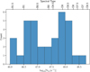 |
Fig. 6 Spectral types and Lyman continuum photon rates of the H II regions derived from the VLA-D radio continuum data. |
4.2 Distribution of cold dust clumps
To investigate the cold dust emission toward G358.69+0.03, we used the ATLASGAL CSC by Urquhart et al. (2014). At the submillimeter wavelength of 870 μm, the thermal emission from dust is considered to be optically thin and contribution from free-free emission should be negligible. This makes ATLASGAL an excellent tool for studying the cold dust clumps that harbor star formation and estimating the column density and total clump mass. The CSC provides a database of ~10 163 cold and massive dense clumps toward the inner Galaxy, which also includes samples of the earliest embedded stages of high-mass star formation activity (Urquhart et al. 2014). We extracted all the sources from the CSC and identified approximately 50 cold dust clumps in our target region. The left panel of Fig. 7 presents the distribution of these dense clumps relative to the radio emission and the FIR maps from the Herschel Hi-GAL survey (Molinari et al. 2016). Although we cannot confirm distances for the ATLASGAL clumps directly, in Sect. 4.4 we present velocity-resolved SiO observations that demonstrate these clumps are kinematically associated with the G358.69+0.03 region. It is evident that the majority of cold dust clumps are concentrated toward the south and southeast of the G358.69+0.03 complex. Only five cH II regions are associated with an ATLASGAL counterpart within a search radius of 18″.
We also investigated emission from Hi-GAL (Molinari et al. 2016), which traces the earliest stages of star formation by tracing emission from cold dust (T < 20 K) in the Milky Way (Elia et al. 2017). To study the distribution of Hi-GAL cold dust clumps, we used the Hi-GAL CSC by Elia et al. (2021). The heliocentric radial velocities and distances to these Hi-GAL clumps were estimated by Mège et al. (2021), using starbird, a Python program utilizing the VIALACTEA Knowledge Base (VLKB; Mège et al. 2021). We extracted all sources from the Hi-GAL CSC (Elia et al. 2021) toward the direction of G358.69+0.03 that had a distance between 8 and 9 kpc, and we obtained 25 Hi-GAL clumps. The distribution of these clumps is shown in the right panel of Fig. 7. We notice a higher concentration of these cold clumps toward the south and southeast directions of G358.69+0.03, similar to that of ATLASGAL clumps. We also investigated the star formation activity in these Hi-GAL clumps using the evolutionary classification discussed in Elia et al. (2021). The clumps were classified into the following categories: “protostellar” clumps, which contain active star formation activity, and quiescent “starless” clumps, based on the presence and absence of 70 μm emission. The starless clumps were further subclassified as gravitationally bound “pre-stellar” and unbound clumps using Larson’s third law (Elia et al. 2021). The gravitationally bound pre-stellar clumps have masses, M(r) > 460 M⊙ (r/pc)1.9 at radii r. Figure 8 shows the bolometric luminosity versus mass of Hi–GAL clumps toward our target region. The temperature of these clumps ranges from ~9–29 K. A majority of these clumps are pre-stellar and a very few are protostellar clumps harboring active high-mass star formation.
The 350 μm cold dust emission is extended and patchy across the region. Within the arc-like distribution of compact H II regions, the 350 μm emission is relatively faint or absent, while the brightest clumps are concentrated outside the arc, particularly toward the south and southeast (see the left panel of Fig. 7). This morphology suggests that the immediate surroundings of the H II regions are relatively depleted in cold dust, consistent with heating and dispersal by massive star formation activity, although we refrain from claiming a strict quantitative anticorrelation.
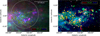 |
Fig. 7 Left: distribution of the ATLASGAL dust continuum sources (gold markers) overlaid on top of the color composite image of G358.69+0.03. The VLA-D+Effelsberg image is shown in red and the Hi-GAL 350 and 70 μm emission maps in green and blue, respectively. The dashed white circle shows G358.69+0.03. Right: color composite image showing the VLA-D image in red and Spitzer bands of 24 and 8 μm in green and blue, respectively. The dashed white partial circles mark the arc-like or U-shaped morphology of the target region. The black circles represent the H II regions identified in this work, and the gold diamonds mark the position of ATLASGAL cold dust clumps toward G358.69+0.03. The gray, violet, and green crosses mark the positions of pre-stellar clumps, protostellar clumps, and gravitationally unbound starless Hi-GAL clumps, respectively, at a distance of 8–9 kpc toward G358.69+0.03. |
4.3 Mid-infrared emission from dust, PAHs, and shocks
The MIR emission maps are valuable for distinguishing between various components in star-forming regions, such as stars, dust continuum emission, PAH emission, and shocked gas (e.g., Smith et al. 2010). To investigate the properties of warm dust emission in G358.69+0.03, we utilized Spitzer IRAC MIR maps at three wavelength bands: 3.6, 4.5, and 8.0 μm. The MIR color composite image (8.0 μm: red, 4.5 μm: green and 3.6 μm: blue) is presented in Fig. 1. In addition to the detection of emission associated with compact H II regions, we observe large-scale diffuse emission at 8 μm spanning ~71.5 pc. This large-scale emission exhibits a broken shell-like morphology that closely aligns with the distribution of cH II regions (see Fig. 2), suggesting a potential association. The 8 μm emission may also include contributions from PAH molecules in the photodissociation regions (Leger & Puget 1984; Churchwell et al. 2009). The observed MIR shell-like structure points to an origin related to stellar feedback, such as stellar wind bubbles, evolved H II regions where the ionized gas has expanded and is interacting with the ambient interstellar medium, or supernova remnants (e.g., Reach et al. 2006; Watson et al. 2008; Deharveng et al. 2010; Pinheiro Gonçalves et al. 2011). We explore this in detail in Sect. 5.
Apart from the emission from heated dust, the 4.5 μm band also contains shock-excited lines of H2 and CO (Liu et al. 2013, and references therein), making it a useful diagnostic for identifying shocks. To investigate this, we generated a pixel-by-pixel [4.5 μm]/[3.6 μm] flux ratio map for the region. The nearly identical point response functions of these bands (~1.7″) allowed us to forgo any point spread function matching correction. The resultant map is shown in Fig. 9. A flux ratio ≥1.5 is typically associated with shocked regions, whereas stellar sources exhibit flux ratios ≪1.5 (Takami et al. 2010; Veena et al. 2018). From the map, we observe enhanced flux ratios (~2–3) primarily toward the eastern and southeastern portions of the arc, with several peaks aligning with cH II regions. This suggests significant shocked emission from these regions, likely due to stellar winds or the expansion of the H II regions. Apart from the high flux ratios near the peaks of cH II regions, we also observe regions with high flux ratios that lack associated radio emission. These could potentially be due to shocks from objects in early evolutionary phases, where the ionized gas has not yet produced strong radio emission, or alternatively, from shocks in molecular outflows or other dynamic processes in less evolved regions.
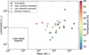 |
Fig. 8 Bolometric luminosity versus mass of Hi-GAL compact sources at distances between 8 and 9 kpc toward G358.69+0.03. The clumps are color-coded by temperature. The markers with thick lines are sources with high reliability parameters taken from Elia et al. (2021). The shapes of the markers (as shown in the legend) indicate different classification categories. The low-mass regime is taken from Saraceno et al. (1996). |
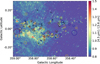 |
Fig. 9 Flux ratio map of Spitzer [4.5 μm]/[3.6 μm] for the target region. The black crosses show the H II regions identified in our work. The maroon, blue, and gold circles mark the known, candidate, and radio-quiet H II regions from the WISE H II catalog. |
4.4 Molecular gas as a tracer of kinematics and shocks
To investigate the large-scale dynamics of the GC and its potential impact on high-mass star formation in G358.69+0.03, we analyzed 12CO(J=3–2) data from the CHIMPS2 survey. Figure 10 shows longitude–velocity (LV) diagrams. In the large-scale LV diagram of the CMZ (Fig. 10a), several well-known features are evident, including the spiral arms at positive velocities, the G1.3 cloud (Busch et al. 2022), and the far dust lane at negative velocities. SgrE is located at the interface of the far dust lane and the CMZ orbit (Anderson et al. 2020; Wallace et al. 2022), coinciding with a prominent stream of high-velocity emission. The zoom-in LV diagram of the G358.69+0.03 region (Fig. 10b) reveals a striking velocity bridge linking the far dust-lane gas (vLSR ≲ −190 km s−1) with the main CMZ component (−180 ≲ vLSR ≲ 0 km s−1). This bridge spans more than 100 km s−1 in velocity and is an indicator of interaction between Galactic bar driven dust lanes and the CMZ (Sormani et al. 2019). The location of compact H II regions in this interface further suggests that the observed massive star formation activity could be related to this dynamical interaction.
To test whether the velocity bridge is indeed associated with shocked gas, we targeted dense clumps south of the arc-like distribution of H II regions (l, b=358.70°, −0.11°; 15′×5′). Within this region, 20 ATLASGAL clumps are cataloged, of which the 17 brightest were observed. We carried out SiO(J=5–4) observations toward these 17 clumps (Fig. 11). SiO is a well-established tracer of shocks, being enhanced both in protostellar outflows and in cloud–cloud collisions (e.g., Gueth et al. 1998; Jiménez-Serra et al. 2010; Kim et al. 2023). SiO emission is detected in 15 out of the 17 clumps, with all detected spectra exhibiting more than one emission component (Fig. B.4). The fitted line parameters are listed in Table B.6. The local standard of rest velocities of the components range between −209.9 and +10.4 km s−1, with line widths spanning 3.2–53.4 km s−1 and an average of ~16 km s−1. Nine clumps exhibit very broad components (>20 km s−1) characteristic of high-velocity shocked gas (e.g., Li et al. 2019). In addition, several spectra display wing-like profiles.
While some of the SiO emission can arise from protostellar outflows, the prevalence of multiple, well-separated velocity components in >65% of the clumps indicates that large-scale shocks, such as those induced by cloud–cloud collisions, must play a significant role in this region. Although the recombination line velocities of 14 known H II regions from Anderson et al. (2020) cluster around −217 to −193 km s−1, the molecular clumps in their vicinity exhibit a much broader spread, extending from −210 to +10 km s−1. Notably, 13 of the 15 SiO-detected clumps exhibit at least one velocity component at vLSR ≤ −120 km s−1, well outside the range of foreground spiral arms (e.g., Reid et al. 2016), confirming their association with the CMZ. A large velocity spread in SiO is a natural outcome in the CMZ, where colliding inflows produce shocked molecular gas at a range of velocities (e.g., Menten et al. 2009).
Under the assumption that the SiO(5–4) emission is optically thin and the gas is under local thermodynamic equilibrium, we estimated the SiO column densities toward individual clumps using the expression (e.g., Kim et al. 2023)
![Mathematical equation: $\[\begin{aligned}N_{\text {tot }}^{\text {thin }}= & \left(\frac{8 \pi \nu^3}{c^3 A_{u l}}\right)\left(\frac{Q(T)}{g_u}\right) \frac{\exp (\frac{E_u}{k_{\mathrm{B}} T_{\mathrm{ex}}})}{\exp (\frac{h \nu}{k_{\mathrm{B}} T_{\mathrm{ex}}})-1} \& \times \frac{1}{\left[J_\nu(T_{\mathrm{ex}})-J_\nu(T_{\mathrm{bg}})\right]} \int \frac{T_{\mathrm{MB}}}{f} d v \& \simeq 1.35 \times 10^{12} \int T_{\mathrm{MB}} ~d v\end{aligned}\]$](/articles/aa/full_html/2026/06/aa54989-25/aa54989-25-eq3.png) (2)
(2)
where ν = 217104.984 MHz is the rest frequency of the SiO J = 5–4 line, c is the speed of light, Aul = 5.296 × 10⁻⁴ s−1 is the Einstein coefficient for spontaneous emission, Q(T) is the partition function, gu is the statistical weight of the upper state level, which is 11 for the (5–4) line, and kB is the Boltzmann constant. The energy of the upper level, Eu is 31.26 K. All these values are taken from Cologne Database for Molecular Spectroscopy (CDMS; Müller et al. 2005). ∫ TMB dv is the integrated intensity and f is the beam filling factor, assumed to be unity. We considered an excitation temperature, Tex, of 25 K, which is equivalent to the average dust temperature in the region obtained from the Herschel PPMAP method (Marsh et al. 2017). The background emission temperature, Tbg is assumed to be 2.7 K corresponding to the cosmic microwave background radiation. The Rayleigh-Jeans temperature, Jν(T) is given by ![Mathematical equation: $\[\frac{h \nu / k_{\mathrm{B}}}{\exp \left(h \nu / k_{\mathrm{b}} T\right)-1}\]$](/articles/aa/full_html/2026/06/aa54989-25/aa54989-25-eq4.png) . Using the above expression we find column densities ranging between 6.8 × 1011 cm−2 and 1.6 × 1013 cm−2. To estimate the abundance of SiO (X(SiO)) with respect to H2, that is, N(SiO)/N(H2), we used the column density map of the region produced from the Herschel data (70–500 μm) using the PPMAP method (Marsh et al. 2017). The SiO abundances given in Table 1 range from 5.3 × 10⁻¹² to 2.6 × 10⁻¹⁰ with a median abundance of 3.8 × 10⁻¹¹. Obtained SiO column densities and abundances are typical of Galactic clouds with SiO detection (e.g., Csengeri et al. 2016; Kim et al. 2023).
. Using the above expression we find column densities ranging between 6.8 × 1011 cm−2 and 1.6 × 1013 cm−2. To estimate the abundance of SiO (X(SiO)) with respect to H2, that is, N(SiO)/N(H2), we used the column density map of the region produced from the Herschel data (70–500 μm) using the PPMAP method (Marsh et al. 2017). The SiO abundances given in Table 1 range from 5.3 × 10⁻¹² to 2.6 × 10⁻¹⁰ with a median abundance of 3.8 × 10⁻¹¹. Obtained SiO column densities and abundances are typical of Galactic clouds with SiO detection (e.g., Csengeri et al. 2016; Kim et al. 2023).
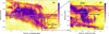 |
Fig. 10 Left: kinematics of the GC region revealed by the 12CO(3–2) longitude-velocity diagram. Right: zoomed-in view of the LV diagram of the G358.69+0.03 region (l~ −1.3° or 358.7°). Cyan stars correspond to the 57 components of the SiO emission detected toward the 15 ATLASGAL clumps listed in Table B.6. The scale bar corresponds to the assumed GC distance of 8.2 kpc. |
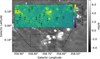 |
Fig. 11 Sources observed with the APEX nFLASH230 receiver at a tuning frequency of 230.79 GHz (black crosses) overplotted on the inset flux ratio map of Spitzer [4.5 μm]/[3.6 μm] for the southern part of the target region, G358.69+0.03. The numbers represent the corresponding IDs of the sources given in Table B.6. The background image shows the VLA-D continuum map. |
5 Discussion
From our analysis, it is clear that the G358.69+0.03 region is a particularly special part of the SgrE complex. We identified 35 compact H II regions that follow a characteristic arc-like or U-shaped distribution. Multiwavelength data further reveal that diffuse MIR emission traces the same arc, while cold dust clumps and molecular gas are distributed around it, indicating ongoing star formation across multiple evolutionary stages.
The G358.69+0.03 region lies at the intersection of the far dust lane and the CMZ orbit, a location associated with some of the highest line-of-sight velocities in the Galaxy (Cram et al. 1996). This dynamical environment of the target region is significant because it channels gas inflows along the Galactic bar into the CMZ (Tress et al. 2020; Hatchfield et al. 2021). Similar inflow–CMZ interactions are seen elsewhere in the GC. For example, ALMA observations of the G5 cloud at (ℓ, b) = (+5.4, −0.4) revealed a velocity bridge between components at ~50 and ~150 km s−1, direct evidence of a dust-lane collision (Gramze et al. 2023). The 200 pc high-velocity cloud studied by Veena et al. (2024), interpreted as near-side dust-lane material overshooting after brushing the CMZ, shows widespread SiO emission and ongoing massive star formation. In contrast, the G1.3 cloud, another dust-lane accretion site, shows no associated star formation activity (Busch et al. 2022). These comparisons highlight that dust-lane termination points can play diverse roles in regulating star formation, depending on the local conditions of the inflow–orbit interaction.
SiO column densities and relative abundances.
5.1 Evidence of a dust-lane–CMZ interaction in G358.69+0.03
To investigate the interplay of large-scale gas inflow and dynamical interactions in G358.69+0.03, we constructed a color-composite image (see the left panel of Fig. 12). The map reveals that most of the high-velocity CO emission is concentrated around the arc-like distribution of H II regions and the central cavity-like area enclosed by the arc. In contrast, the lower-velocity emission is predominantly located to the east and southeast of the H II arc, with only partial overlap with the far dust-lane component. Strikingly, the majority of the compact H II regions and ATLASGAL clumps (see Fig. 7) are found precisely at this overlap zone, strongly suggesting that their formation is linked to the dynamical interaction between the two velocity components.
To quantify this spatial correspondence, we constructed an additional LV diagram along the slanted line AB, which intersects the high-velocity far dust-lane emission, the lower-velocity CMZ gas, and their overlap region. The resulting diagram is shown in the right panel of Fig. 12. In this LV diagram, we observe a characteristic J-shaped (or hook-like) feature that links the two velocity components. The coincidence of this kinematic bridge with the location of the H II regions provides strong evidence that the arc-like distribution of massive stars in G358.69+0.03 formed at the interface where the far dust-lane inflow terminates and collides with the CMZ stream.
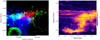 |
Fig. 12 Left: three-color map of the SgrE region. Red shows 12CO(J=3–2) emission integrated over −240 to −190 km s−1, tracing the far dust-lane component; blue shows −185 to −50 km s−1, tracing the main CMZ stream and the emission bridge observed in Fig. 10b; and green corresponds to the MeerKAT 1 GHz image, tracing the H II regions. The dashed line (AB) indicates the cut used to construct the LV diagram. Right: 12CO(J=3–2) LV diagram along the AB line, revealing a velocity bridge linking the far dust-lane gas with the CMZ stream, consistent with a site of cloud-cloud interaction. |
5.2 Morphology of the target region
Our kinematic analysis suggests that the morphology of G358.69+0.03 is a result of large-scale dynamical interactions. We investigated the two following scenarios in a bid to explain the morphology.
Feedback scenario: The structured star formation initially resembles an evolved feedback structure, such as an expanding H II region or supernova remnant, in which stellar feedback drives shell expansion and triggers secondary star formation at the rim (e.g., Zavagno et al. 2005; Koo et al. 2008). However, we could not find any evidence of a supernova remnant in this region. To further test the feedback scenario, we estimated the flux density of the large-scale ionized shell using the GLOSTAR VLA+Effelsberg map at 5.8 GHz, after subtracting diffuse background emission and compact sources. The total flux of 49 Jy corresponds to a Lyman continuum photon rate of 3.7 × 1050 s−1, consistent with ionization by an extremely massive O3-type star or a small OB cluster. If such a source existed, the expansion of an older H II region could in principle have compressed the surrounding molecular gas and triggered a new burst of star formation, consistent with sequential star-formation models. However, we find no direct observational evidence of a coherent expanding shell, and the recombination and supernova timescales (≲105 yr) are too short to account for the currently observed population of compact H II regions.
Could-cloud collisions scenario: On the other hand, the dynamical ages of the compact H II regions (0.06–1 Myr) are consistent with the 105–106 yr timescales expected for massive star formation triggered by cloud–cloud collisions (e.g., Torii et al. 2011). The diffuse radio shell is therefore more plausibly explained as leakage of ionizing photons from the compact H II region complexes themselves, as observed in other Galactic star-forming regions (e.g., Luisi et al. 2017). This scenario is summarized in Fig. 13, which illustrates the inflow of gas along the near- and far-side dust lanes. Both lanes feed material into the CMZ, with G358.69+0.03 region located exactly at the critical intersection between the far dust lane and the CMZ orbit. At this termination point, as the shock wave moves outward from the point of collision, it can trigger widespread star formation in the compressed gas, leading to the formation of H II regions along the shock front. Numerical models of colliding clouds (Habe & Ohta 1992; Takahira et al. 2014; Fukui et al. 2021) also show that collisions between clouds of unequal density produce arc- or U-shaped compressed layers, with massive star formation occurring preferentially along the rim. This is consistent with the observed morphology of G358.69+0.03: a curved arc of compact H II regions, diffuse ionized gas filling the arc, and strong shock signatures traced by SiO.
Cloud–cloud collision-driven star formation has been observed in many nearby interacting galaxies, including the Magellanic System and the Antennae Galaxies, as well as in almost all well-known high-mass star-forming regions in the Milky Way (Fukui et al. 2021). In the GC, Enokiya & Fukui (2022) investigated the effects of cloud-cloud collisions in the Sgr B region, one of the most active star-forming regions in the Galaxy. Their analysis revealed clear signatures of cloud-cloud collision, which they interpreted as the trigger for the vigorous star formation activity in the region.
The cloud–cloud collision scenario provides a compelling explanation for both the morphology and the kinematics of G358.60+0.03. Furthermore, G358.69+0.03 marks the site where the far dust-lane inflow collides with the CMZ orbit, making it the key interaction zone within the broader SgrE complex. This subregion thus provides a unique laboratory for studying how large-scale bar-driven gas inflows directly shape the morphology and trigger the formation of massive stars in the CMZ.
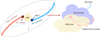 |
Fig. 13 Schematic illustration of gas inflow into the CMZ. Left: gas streams along the near- and far-side dust lanes feed the CMZ. Sgr E is located at the intersection of the far dust lane and the CMZ orbit (adapted from Henshaw et al. 2023). Right: zoomed-in view of the collision, where the far dust lane impacts the CMZ gas, compressing material and producing an arc-like or U-shaped distribution of H II regions. |
6 Conclusions
The G358.69+0.03 subregion of the Sgr E star-forming complex exhibits an intriguing arc-like morphology that is traced by diffuse 8 μm emission and a U-shaped distribution of compact radio and infrared sources. Using GLOSTAR 5.8 GHz VLA-D data, we identified 49 compact radio sources, 35 of which we classified as H II regions based on their spectral indices, associations with MIR or FIR sources, and corresponding cold dust emission. Among these, 27 were previously cataloged in the WISE V2.3 catalog (Anderson et al. 2014), while 3 additional radio counterparts are identified for previous “radio-quiet” WISE H II regions and 5 new cH II regions are reported. The derived spectral types span O6.5 to B1.5, with dynamical ages ranging from 0.06 to 1.05 Myr. We identified around 50 cold dust clumps in the region, primarily concentrated toward the south and southeast of the U-shaped H II region distribution, with evolutionary classifications ranging from pre-stellar to protostellar. The cold dust emission is relatively faint within the arc of compact H II regions, suggesting that massive star formation has already begun to alter the immediate environment, and active clump formation continues along the periphery. The MIR flux ratio maps reveal evidence of shocked emission, which is supported by widespread SiO detections in dense clumps. The SiO components span a broad velocity range and align with a continuous velocity bridge in CO, linking the high-velocity far dust-lane gas with the main CMZ stream.
Given the location of G358.69+0.03 at the intersection of the far-side dust lane and the CMZ orbit, these results suggest that the observed star formation activity is shaped by large-scale dynamical interactions. The combination of high-velocity gas, shock tracers, and the arc-like distribution of H II regions is difficult to explain through stellar feedback alone. Instead, the evidence favors a scenario in which the collision between dust-lane inflow and the CMZ stream has compressed the gas and triggered massive star formation.
Acknowledgements
We would like to express our deepest gratitude to Prof. Dr. Karl Martin Menten for his guidance, and unwavering support and trust throughout this research. We thank the referees for the valuable comments and suggestions that improved the quality of the paper. This research was partially funded by the ERC Advanced Investigator Grant GLOSTAR (247078). A.C. acknowledges the support by the Deutsche Forschungsgemeinschaft (DFG, German Research Foundation) – Project-ID 500700252 – SFB 1601. This research has made use of the NASA/IPAC Infrared Science Archive, which is funded by the National Aeronautics and Space Administration and operated by the California Institute of Technology. This study utilized Astropy (Astropy Collaboration 2022), SAOImage DS9 (Joye & Mandel 2003), APLpy (Robitaille & Bressert 2012), GIlDAS (Pety 2005) and CASA (CASA Team 2022). This document was prepared using the collaborative tool Overleaf available at: https://www.overleaf.com/. We thank S.-N.X. Medina for her support during the observation campaigns with Effelsberg. S.A.D. acknowledges the M2FINDERS project from the European Research Council (ERC) under the European Union’s Horizon 2020 research and innovation programme (grant No 101018682). Y.G. was supported by the Ministry of Science and Technology of China under the National Key R&D Program under grant No. 2023YFA1608200, the National Natural Science Foundation of China (NSFC) under grant No. 12427901, and the Strategic Priority Research Program of the Chinese Academy of Sciences under grant No. XDB0800301.
References
- Aguirre, J. E., Ginsburg, A. G., Dunham, M. K., et al. 2011, ApJS, 192, 4 [Google Scholar]
- Anderson, L. D., Zavagno, A., Barlow, M. J., García-Lario, P., & Noriega-Crespo, A. 2012, A&A, 537, A1 [NASA ADS] [CrossRef] [EDP Sciences] [Google Scholar]
- Anderson, L. D., Bania, T. M., Balser, D. S., et al. 2014, ApJS, 212, 1 [Google Scholar]
- Anderson, L. D., Sormani, M. C., Ginsburg, A., et al. 2020, ApJ, 901, 51 [NASA ADS] [CrossRef] [Google Scholar]
- Armentrout, W. P., Anderson, L. D., Balser, D. S., et al. 2017, ApJ, 841, 121 [Google Scholar]
- Astropy Collaboration (Price-Whelan, A. M., et al.) 2022, ApJ, 935, 167 [NASA ADS] [CrossRef] [Google Scholar]
- Balser, D. S., Rood, R. T., Bania, T. M., & Anderson, L. D. 2011, ApJ, 738, 27 [NASA ADS] [CrossRef] [Google Scholar]
- Barnes, A. T., Longmore, S. N., Battersby, C., et al. 2017, MNRAS, 469, 2263 [Google Scholar]
- Battersby, C., Walker, D. L., Barnes, A., et al. 2025, ApJ, 984, 156 [Google Scholar]
- Becker, R. H., White, R. L., Helfand, D. J., & Zoonematkermani, S. 1994, ApJS, 91, 347 [Google Scholar]
- Benjamin, R. A., Churchwell, E., Babler, B. L., et al. 2003, PASP, 115, 953 [Google Scholar]
- Bertin, E., & Arnouts, S. 1996, A&AS, 117, 393 [NASA ADS] [CrossRef] [EDP Sciences] [Google Scholar]
- Beuther, H., Bihr, S., Rugel, M., et al. 2016, A&A, 595, A32 [NASA ADS] [CrossRef] [EDP Sciences] [Google Scholar]
- Brunthaler, A., Menten, K. M., Dzib, S. A., et al. 2021, A&A, 651, A85 [EDP Sciences] [Google Scholar]
- Busch, L. A., Riquelme, D., Güsten, R., et al. 2022, A&A, 668, A183 [NASA ADS] [CrossRef] [EDP Sciences] [Google Scholar]
- Carey, S. J., Noriega-Crespo, A., Mizuno, D. R., et al. 2009, PASP, 121, 76 [Google Scholar]
- CASA Team (Bean, B., et al.) 2022, PASP, 134, 114501 [NASA ADS] [CrossRef] [Google Scholar]
- Churchwell, E., Brian, B., Bania, T., et al. 2005, GLIMPSE II: Imaging the Central +/-10 Degrees of the Galactic Plane with IRAC, Spitzer Proposal ID 20201 [Google Scholar]
- Churchwell, E., Babler, B. L., Meade, M. R., et al. 2009, PASP, 121, 213 [Google Scholar]
- Condon, J. J., & Ransom, S. M. 2016, Essential Radio Astronomy [Google Scholar]
- Cotton, W. D. 2008, PASP, 120, 439 [Google Scholar]
- Cram, L. E., Claussen, M. J., Beasley, A. J., Gray, A. D., & Goss, W. M. 1996, MNRAS, 280, 1110 [Google Scholar]
- Csengeri, T., Leurini, S., Wyrowski, F., et al. 2016, A&A, 586, A149 [NASA ADS] [CrossRef] [EDP Sciences] [Google Scholar]
- Cutri, R. M., Skrutskie, M. F., van Dyk, S., et al. 2003, 2MASS All Sky Catalog of point sources. [Google Scholar]
- Deharveng, L., Schuller, F., Anderson, L. D., et al. 2010, A&A, 523, A6 [NASA ADS] [CrossRef] [EDP Sciences] [Google Scholar]
- Deharveng, L., Zavagno, A., Samal, M. R., et al. 2015, A&A, 582, A1 [NASA ADS] [CrossRef] [EDP Sciences] [Google Scholar]
- Dokara, R., Gong, Y., Reich, W., et al. 2023, A&A, 671, A145 [NASA ADS] [CrossRef] [EDP Sciences] [Google Scholar]
- Dyson, J. E., & Williams, D. A. 1980, Physics of the Interstellar Medium [Google Scholar]
- Dzib, S. A., Yang, A. Y., Urquhart, J. S., et al. 2023, A&A, 670, A9 [NASA ADS] [CrossRef] [EDP Sciences] [Google Scholar]
- Eden, D. J., Moore, T. J. T., Currie, M. J., et al. 2020, MNRAS, 498, 5936 [NASA ADS] [CrossRef] [Google Scholar]
- Elia, D., Molinari, S., Schisano, E., et al. 2017, MNRAS, 471, 100 [NASA ADS] [CrossRef] [Google Scholar]
- Elia, D., Merello, M., Molinari, S., et al. 2021, MNRAS, 504, 2742 [NASA ADS] [CrossRef] [Google Scholar]
- Enokiya, R., & Fukui, Y. 2022, ApJ, 931, 155 [CrossRef] [Google Scholar]
- Ferrière, K., Gillard, W., & Jean, P. 2007, A&A, 467, 611 [NASA ADS] [CrossRef] [EDP Sciences] [Google Scholar]
- Fukui, Y., Habe, A., Inoue, T., Enokiya, R., & Tachihara, K. 2021, PASJ, 73, S1 [Google Scholar]
- Ginsburg, A., Henkel, C., Ao, Y., et al. 2016, A&A, 586, A50 [NASA ADS] [CrossRef] [EDP Sciences] [Google Scholar]
- Glimpse Team 2020, GLIMPSE II Epoch1 Catalog, NASA IPAC DataSet, IRSA227 [Google Scholar]
- Gramze, S. R., Ginsburg, A., Meier, D. S., et al. 2023, ApJ, 959, 93 [NASA ADS] [CrossRef] [Google Scholar]
- GRAVITY Collaboration (Abuter, R., et al.) 2019, A&A, 625, L10 [NASA ADS] [CrossRef] [EDP Sciences] [Google Scholar]
- Gray, A. D. 1994, MNRAS, 270, 822 [Google Scholar]
- Gray, A. D., Whiteoak, J. B. Z., Cram, L. E., & Goss, W. M. 1993, MNRAS, 264, 678 [Google Scholar]
- Gueth, F., Guilloteau, S., & Bachiller, R. 1998, A&A, 333, 287 [NASA ADS] [Google Scholar]
- Güsten, R., Nyman, L. Å., Schilke, P., et al. 2006, A&A, 454, L13 [NASA ADS] [CrossRef] [EDP Sciences] [Google Scholar]
- Gutermuth, R. A., & Heyer, M. 2020, MIPSGAL 24 micron Catalog, NASA IPAC DataSet, IRSA258 [Google Scholar]
- Habe, A., & Ohta, K. 1992, PASJ, 44, 203 [NASA ADS] [Google Scholar]
- Hales, C. A., Murphy, T., Curran, J. R., et al. 2012, MNRAS, 425, 979 [Google Scholar]
- Hatchfield, H. P., Sormani, M. C., Tress, R. G., et al. 2021, ApJ, 922, 79 [NASA ADS] [CrossRef] [Google Scholar]
- Hatchfield, H. P., Battersby, C., Barnes, A. T., et al. 2024, ApJ, 962, 14 [Google Scholar]
- Henney, W. J., Tarango-Yong, J. A., Ángel Gutiérrez-Soto, L., & Arthur, S. J. 2019, MNRAS, submitted [arXiv:1907.00122] [Google Scholar]
- Henshaw, J. D., Longmore, S. N., Kruijssen, J. M. D., et al. 2016, MNRAS, 457, 2675 [Google Scholar]
- Henshaw, J. D., Barnes, A. T., Battersby, C., et al. 2023, in Astronomical Society of the Pacific Conference Series, 534, Protostars and Planets VII, eds. S. Inutsuka, Y. Aikawa, T. Muto, K. Tomida, & M. Tamura, 83 [Google Scholar]
- Heywood, I., Rammala, I., Camilo, F., et al. 2022, ApJ, 925, 165 [NASA ADS] [CrossRef] [Google Scholar]
- Hi-GAL Team. 2020a, Hi-GAL 160 micron Photometric Catalog, NASA IPAC DataSet, IRSA25 [Google Scholar]
- Hi-GAL Team. 2020b, Hi-GAL 250 micron Photometric Catalog, NASA IPAC DataSet, IRSA24 [Google Scholar]
- Hi-GAL Team. 2020c, Hi-GAL 350 micron Photometric Catalog, NASA IPAC DataSet, IRSA28 [Google Scholar]
- Hi-GAL Team. 2020d, Hi-GAL 500 micron Photometric Catalog, NASA IPAC DataSet, IRSA26 [Google Scholar]
- Hi-GAL Team. 2020e, Hi-GAL 70 micron Photometric Catalog, NASA IPAC DataSet, IRSA27 [Google Scholar]
- Hoare, M. G., Purcell, C. R., Churchwell, E. B., et al. 2012, PASP, 124, 939 [Google Scholar]
- Jiménez-Serra, I., Caselli, P., Tan, J. C., et al. 2010, MNRAS, 406, 187 [Google Scholar]
- Joye, W. A., & Mandel, E. 2003, in Astronomical Society of the Pacific Conference Series, 295, Astronomical Data Analysis Software and Systems XII, eds. H. E. Payne, R. I. Jedrzejewski, & R. N. Hook, 489 [Google Scholar]
- Khan, S., Rugel, M. R., Brunthaler, A., et al. 2024, A&A, 689, A81 [NASA ADS] [CrossRef] [EDP Sciences] [Google Scholar]
- Kim, W. J., Urquhart, J. S., Veena, V. S., et al. 2023, A&A, 679, A123 [NASA ADS] [CrossRef] [EDP Sciences] [Google Scholar]
- Koepferl, C. M., Robitaille, T. P., Morales, E. F. E., & Johnston, K. G. 2015, ApJ, 799, 53 [Google Scholar]
- Koo, B.-C., McKee, C. F., Lee, J.-J., et al. 2008, ApJ, 673, L147 [Google Scholar]
- Kwan, J. 1997, ApJ, 489, 284 [Google Scholar]
- Leger, A., & Puget, J. L. 1984, A&A, 137, L5 [Google Scholar]
- Li, S., Wang, J., Fang, M., et al. 2019, ApJ, 878, 29 [NASA ADS] [CrossRef] [Google Scholar]
- Liszt, H. S. 1992, ApJS, 82, 495 [Google Scholar]
- Liu, T., Wu, Y., & Zhang, H. 2013, ApJ, 776, 29 [Google Scholar]
- Longmore, S. N., Bally, J., Testi, L., et al. 2013, MNRAS, 429, 987 [NASA ADS] [CrossRef] [Google Scholar]
- Lucas, P. W., Hoare, M. G., Longmore, A., et al. 2008, MNRAS, 391, 136 [Google Scholar]
- Luisi, M., Anderson, L. D., Balser, D. S., Wenger, T. V., & Bania, T. M. 2017, ApJ, 849, 117 [Google Scholar]
- Mackey, J., Langer, N., & Gvaramadze, V. V. 2013, MNRAS, 436, 859 [NASA ADS] [CrossRef] [Google Scholar]
- Marsh, K. A., Whitworth, A. P., Lomax, O., et al. 2017, MNRAS, 471, 2730 [Google Scholar]
- Marshall, D. J., Fux, R., Robin, A. C., & Reylé, C. 2008, A&A, 477, L21 [NASA ADS] [CrossRef] [EDP Sciences] [Google Scholar]
- Matsakis, D. N., Evans, II, N. J., Sato, T., & Zuckerman, B. 1976, AJ, 81, 172 [Google Scholar]
- McMullin, J. P., Waters, B., Schiebel, D., Young, W., & Golap, K. 2007, in Astronomical Society of the Pacific Conference Series, 376, Astronomical Data Analysis Software and Systems XVI, eds. R. A. Shaw, F. Hill, & D. J. Bell, 127 [Google Scholar]
- Medina, S. N. X., Urquhart, J. S., Dzib, S. A., et al. 2019, A&A, 627, A175 [NASA ADS] [CrossRef] [EDP Sciences] [Google Scholar]
- Medina, S.-N. X., Dzib, S. A., Urquhart, J. S., et al. 2024, A&A, 689, A196 [NASA ADS] [CrossRef] [EDP Sciences] [Google Scholar]
- Mège, P., Russeil, D., Zavagno, A., et al. 2021, A&A, 646, A74 [NASA ADS] [CrossRef] [EDP Sciences] [Google Scholar]
- Meng, F., Sánchez-Monge, Á., Schilke, P., et al. 2019, A&A, 630, A73 [NASA ADS] [CrossRef] [EDP Sciences] [Google Scholar]
- Meng, F., Sánchez-Monge, Á., Schilke, P., et al. 2022, A&A, 666, A31 [NASA ADS] [CrossRef] [EDP Sciences] [Google Scholar]
- Menten, K. M., Wilson, R. W., Leurini, S., & Schilke, P. 2009, ApJ, 692, 47 [NASA ADS] [CrossRef] [Google Scholar]
- Mezger, P. G., & Henderson, A. P. 1967, ApJ, 147, 471 [Google Scholar]
- Molinari, S., Bally, J., Glover, S., et al. 2014, in Protostars and Planets VI, eds. H. Beuther, R. S. Klessen, C. P. Dullemond, & T. Henning, 125 [Google Scholar]
- Molinari, S., Schisano, E., Elia, D., et al. 2016, A&A, 591, A149 [NASA ADS] [CrossRef] [EDP Sciences] [Google Scholar]
- Müller, H. S. P., Schlöder, F., Stutzki, J., & Winnewisser, G. 2005, J. Mol. Struct., 742, 215 [Google Scholar]
- Nandakumar, G., Veena, V. S., Vig, S., et al. 2016, AJ, 152, 146 [Google Scholar]
- Nguyen, H., Rugel, M. R., Menten, K. M., et al. 2021, A&A, 651, A88 [NASA ADS] [CrossRef] [EDP Sciences] [Google Scholar]
- Padovani, M., Marcowith, A., Sánchez-Monge, Á., Meng, F., & Schilke, P. 2019, A&A, 630, A72 [NASA ADS] [CrossRef] [EDP Sciences] [Google Scholar]
- Panagia, N. 1973, AJ, 78, 929 [NASA ADS] [CrossRef] [Google Scholar]
- Panja, A., Sun, Y., Chen, W. P., & Mondal, S. 2022, ApJ, 939, 46 [Google Scholar]
- Paron, S., Petriella, A., & Ortega, M. E. 2011, A&A, 525, A132 [NASA ADS] [CrossRef] [EDP Sciences] [Google Scholar]
- Pety, J. 2005, in SF2A-2005: Semaine de l’Astrophysique Francaise, eds. F. Casoli, T. Contini, J. M. Hameury, & L. Pagani, 721 [Google Scholar]
- Pinheiro Gonçalves, D., Noriega-Crespo, A., Paladini, R., Martin, P. G., & Carey, S. J. 2011, AJ, 142, 47 [Google Scholar]
- Purcell, C. R., Hoare, M. G., Cotton, W. D., et al. 2013, ApJS, 205, 1 [Google Scholar]
- Reach, W. T., Rho, J., Tappe, A., et al. 2006, AJ, 131, 1479 [NASA ADS] [CrossRef] [Google Scholar]
- Reid, M. J., Dame, T. M., Menten, K. M., & Brunthaler, A. 2016, ApJ, 823, 77 [Google Scholar]
- Robitaille, T., & Bressert, E. 2012, APLpy: Astronomical Plotting Library in Python, Astrophysics Source Code Library [record ascl:1208.017] [Google Scholar]
- Roman-Duval, J., Heyer, M., Brunt, C. M., et al. 2016, ApJ, 818, 144 [NASA ADS] [CrossRef] [Google Scholar]
- Saraceno, P., Andre, P., Ceccarelli, C., Griffin, M., & Molinari, S. 1996, A&A, 309, 827 [Google Scholar]
- Schilke, P., Walmsley, C. M., Pineau des Forets, G., & Flower, D. R. 1997, A&A, 321, 293 [NASA ADS] [Google Scholar]
- Schmiedeke, A., Schilke, P., Möller, T., et al. 2016, A&A, 588, A143 [NASA ADS] [CrossRef] [EDP Sciences] [Google Scholar]
- Schuller, F., Menten, K. M., Contreras, Y., et al. 2009, A&A, 504, 415 [NASA ADS] [CrossRef] [EDP Sciences] [Google Scholar]
- Shetty, R., Beaumont, C. N., Burton, M. G., Kelly, B. C., & Klessen, R. S. 2012, MNRAS, 425, 720 [Google Scholar]
- Simpson, R. J., Povich, M. S., Kendrew, S., et al. 2012, MNRAS, 424, 2442 [NASA ADS] [CrossRef] [Google Scholar]
- Skrutskie, M. F., Cutri, R. M., Stiening, R., et al. 2003, 2MASS All-Sky Point Source Catalog, NASA IPAC DataSet, IRSA2 [Google Scholar]
- Skrutskie, M. F., Cutri, R. M., Stiening, R., et al. 2006, AJ, 131, 1163 [NASA ADS] [CrossRef] [Google Scholar]
- Smith, N., Povich, M. S., Whitney, B. A., et al. 2010, MNRAS, 406, 952 [Google Scholar]
- Sormani, M. C., & Barnes, A. T. 2019, MNRAS, 484, 1213 [NASA ADS] [CrossRef] [Google Scholar]
- Sormani, M. C., Treß, R. G., Glover, S. C. O., et al. 2019, MNRAS, 488, 4663 [NASA ADS] [CrossRef] [Google Scholar]
- Strömgren, B. 1939, ApJ, 89, 526 [CrossRef] [Google Scholar]
- Takahira, K., Tasker, E. J., & Habe, A. 2014, ApJ, 792, 63 [Google Scholar]
- Takami, M., Karr, J. L., Koh, H., Chen, H.-H., & Lee, H.-T. 2010, ApJ, 720, 155 [Google Scholar]
- Tenorio-Tagle, G. 1979, A&A, 71, 59 [NASA ADS] [Google Scholar]
- Torii, K., Enokiya, R., Sano, H., et al. 2011, ApJ, 738, 46 [NASA ADS] [CrossRef] [Google Scholar]
- Tress, R. G., Sormani, M. C., Glover, S. C. O., et al. 2020, MNRAS, 499, 4455 [NASA ADS] [CrossRef] [Google Scholar]
- Urquhart, J. S., Thompson, M. A., Moore, T. J. T., et al. 2013, MNRAS, 435, 400 [Google Scholar]
- Urquhart, J. S., Csengeri, T., Wyrowski, F., et al. 2014, A&A, 568, A41 [NASA ADS] [CrossRef] [EDP Sciences] [Google Scholar]
- Veena, V. S., Vig, S., Tej, A., et al. 2016, MNRAS, 456, 2425 [Google Scholar]
- Veena, V. S., Vig, S., Mookerjea, B., et al. 2018, ApJ, 852, 93 [Google Scholar]
- Veena, V. S., Kim, W. J., Sánchez-Monge, Á., et al. 2024, A&A, 689, A121 [NASA ADS] [CrossRef] [EDP Sciences] [Google Scholar]
- Wallace, J., Battersby, C., Mills, E. A. C., et al. 2022, ApJ, 939, 58 [NASA ADS] [CrossRef] [Google Scholar]
- Watson, C., Povich, M. S., Churchwell, E. B., et al. 2008, ApJ, 681, 1341 [Google Scholar]
- White, R. L., Becker, R. H., & Helfand, D. J. 2005, AJ, 130, 586 [NASA ADS] [CrossRef] [Google Scholar]
- WISE Team. 2020, WISE All-Sky Source Catalog, NASA IPAC DataSet, IRSA142 [Google Scholar]
- Wright, E. L., Eisenhardt, P. R. M., Mainzer, A. K., et al. 2010, AJ, 140, 1868 [Google Scholar]
- Yang, A. Y., Urquhart, J. S., Thompson, M. A., et al. 2021, A&A, 645, A110 [EDP Sciences] [Google Scholar]
- Yang, A. Y., Dzib, S. A., Urquhart, J. S., et al. 2023, A&A, 680, A92 [NASA ADS] [CrossRef] [EDP Sciences] [Google Scholar]
- Yusef-Zadeh, F., Hewitt, J. W., Arendt, R. G., et al. 2009, ApJ, 702, 178 [Google Scholar]
- Zavagno, A., Deharveng, L., Brand, J., et al. 2005, in IAU Symposium, 227, Massive Star Birth: A Crossroads of Astrophysics, eds. R. Cesaroni, M. Felli, E. Churchwell, & M. Walmsley, 346 [Google Scholar]
Appendix A Properties of H II regions
We estimated the physical properties of H II regions using the Strömgen sphere approximation, i.e., a fully ionized spherical region of uniform electron density and devoid of any interstellar dust. We also assumed the emission to be homogeneous and optically thin. The main source of radio flux from an H II region is the free-free thermal emission known as the bremsstrahlung radiation (Condon & Ransom 2016). The Lyman continuum luminosity (Nly), which represents the flux of ionizing photons emitted by the central massive star, is directly correlated with the stellar mass. The more massive a star, the higher is the production of ionizing photons and hence higher the values of Nly. Assuming that a single zero age main sequence star is responsible for the ionization of the H II region, we estimated the Lyman continuum photon rate under the assumption of optically thin emission, minimal leakage of photons into the interstellar medium and zero dust attenuation of the UV photons (Panagia 1973; Armentrout et al. 2017; Anderson et al. 2020, and references therein). Nly was calculated using the expression (Matsakis et al. 1976)
![Mathematical equation: $\[\left(\frac{N_{\mathrm{ly}}}{\mathrm{~s}^{-1}}\right)=4.771 \times 10^{42} \times\left(\frac{F_\nu}{\mathrm{Jy}}\right)\left(\frac{T_e}{\mathrm{~K}}\right)^{-0.45}\left(\frac{\nu}{\mathrm{GHz}}\right)^{0.1}\left(\frac{\mathrm{D}}{\mathrm{pc}}\right)^2,\]$](/articles/aa/full_html/2026/06/aa54989-25/aa54989-25-eq5.png) (A.1)
(A.1)
where Fv is the flux density of the H II regions as estimated from the GLOSTAR VLA-D radio continuum image using BLOBCAT. Te is the electron temperature which we assumed to be 6000 K for H II regions near the GC (Balser et al. 2011; Anderson et al. 2020). The frequency ν = 5.8 GHz is the effective frequency of the GLOSTAR integrated intensity map. The distance (D) is taken to be 8.2 kpc (GRAVITY Collaboration 2019). The Nly values are converted to main sequence spectral types using the data compiled in Armentrout et al. (2017).
The effective radius of the cH II regions was estimated using
![Mathematical equation: $\[\left(\frac{R_{\mathrm{H~\small{II}}}}{\mathrm{pc}}\right)=\frac{1}{57.32} \times \sqrt{\frac{n_{\mathrm{pix}} \times(\text { pixel size })^2}{\pi}} \times\left(\frac{\mathrm{D}}{\mathrm{pc}}\right),\]$](/articles/aa/full_html/2026/06/aa54989-25/aa54989-25-eq6.png) (A.2)
(A.2)
where npix is the number of flooded pixels comprising the blob which was taken from the BLOBCAT output catalog. The size of the square pixels chosen to image the VLA-D configuration map was 2.5″. The effective radius ranges from 0.35–3.87 pc. The dynamical age of H II regions referring to the time taken by the H II region to evolve to its current size is estimated using (Dyson & Williams 1980)
![Mathematical equation: $\[t_{\mathrm{dyn}}=\left(\frac{4 R_{\mathrm{s}}}{7 c_{\mathrm{s}}}\right)\left[\left(\frac{R_{\mathrm{H~\small{II}}}}{R_{\mathrm{s}}}\right)^{7 / 4}-1\right],\]$](/articles/aa/full_html/2026/06/aa54989-25/aa54989-25-eq7.png) (A.3)
(A.3)
where RH II is the effective radius of H II region. The velocity of sound in the ionized gas is taken to be cs = 10 km s−1 (Paron et al. 2011), typical for H II regions. The radius of the Strömgen radius (Rs) is estimated using the expression (Strömgren 1939)
![Mathematical equation: $\[R_{\mathrm{s}}=\left(\frac{3 N_{\mathrm{ly}}}{4 \pi n_0^2 \alpha_{\mathrm{B}}}\right)^{1 / 3},\]$](/articles/aa/full_html/2026/06/aa54989-25/aa54989-25-eq8.png) (A.4)
(A.4)
where n0 is the ambient particle number density of the neutral gas which is typically ~103 cm−3 (Panja et al. 2022). The hydrogen radiative recombination coefficient to all levels above the ground is given by αB = 2.6 × 10⁻¹³ (104 K/Te)0.7 cm3 s−1 (Kwan 1997). The dynamical age ranges from 0.07 to 0.94 Myr. The EM of an H II region is defined as ![Mathematical equation: $\[\mathrm{EM} =\int n_{\mathrm{e}}^{2} ~d s\]$](/articles/aa/full_html/2026/06/aa54989-25/aa54989-25-eq9.png) , which is the fundamental quantity relating the electron density along the line of sight (Mezger & Henderson 1967). Assuming constant electron density, this expression simplifies to
, which is the fundamental quantity relating the electron density along the line of sight (Mezger & Henderson 1967). Assuming constant electron density, this expression simplifies to ![Mathematical equation: $\[\mathrm{EM}\text{=}~n_{e}^{2} ~L\]$](/articles/aa/full_html/2026/06/aa54989-25/aa54989-25-eq10.png) , where L is the path length through the region. Following Schmiedeke et al. (2016), and adopting the formulation convenient for flux measurements within circular apertures, we calculated the EM and ne as
, where L is the path length through the region. Following Schmiedeke et al. (2016), and adopting the formulation convenient for flux measurements within circular apertures, we calculated the EM and ne as
![Mathematical equation: $\[\left(\frac{\mathrm{EM}}{\mathrm{pc} \mathrm{~cm}^{-6}}\right)=3.217 \times 10^7 \times\left(\frac{F_\nu}{\mathrm{Jy}}\right)\left(\frac{T_e}{\mathrm{~K}}\right)^{0.35}\left(\frac{\nu}{\mathrm{GHZ}}\right)^{0.1}\left(\frac{\theta_{\text {source }}}{\operatorname{arcsec}}\right)^{-2},\]$](/articles/aa/full_html/2026/06/aa54989-25/aa54989-25-eq11.png) (A.5)
(A.5)
![Mathematical equation: $\[\begin{aligned}\left(\frac{n_{\mathrm{e}}}{\mathrm{~cm}^{-3}}\right)=2.576 \times 10^6 \times\left(\frac{F_\nu}{\mathrm{Jy}}\right)^{0.5}\left(\frac{T_e}{\mathrm{~K}}\right)^{0.175}\left(\frac{\nu}{\mathrm{GHZ}}\right)^{0.05} \\\left(\frac{\theta_{\text {source }}}{\operatorname{arcsec}}\right)^{-1.5}\left(\frac{\mathrm{D}}{\mathrm{pc}}\right)^{-0.5}\end{aligned}\]$](/articles/aa/full_html/2026/06/aa54989-25/aa54989-25-eq12.png) (A.6)
(A.6)
where θsource is the angular diameter of the H II region as estimated using the effective diameter at a distance (D) of 8.2 kpc. Mezger & Henderson (1967) showed that for alternative density distributions (cylindrical or Gaussian), the spherical case provides an upper limit to EM and a lower limit to ne, but is generally consistent with these models. For the purposes of this study, we therefore retained the spherical model as a reasonable approximation, while noting that the true values may fall within the range implied by the different geometries. The EM values range from 2.64 to 35.2 × 10³ pc cm−6 and the ne ranges from 29.48 to 121.20 cm−3.
A.1 Morphology of H II regions and their extended envelopes
The H II regions identified in our study show different morphologies as shown in Fig. A.1. A few regions, such as G358.784+0.060, exhibit a broken shell-like structure, whereas some regions, such as G358.551–0.029 and G358.747–0.154, have a cometary morphology characterized by a cometary head and a low brightness tail. There are several irregular or multiple peaked H II region complexes, like G358.505+0.108, where multiple compact regions are clustered and embedded within a cometary-like low brightness diffuse gas. The H II region G358.632+0.063 is located near the geometric center of the shell and exhibits a distinct morphology. In addition to the central compact source, which has slightly extended emission in the north-south direction, it possesses a characteristic tail extending ~3.7 pc in the southeast-northwest direction. This tail is also prominent in MIR and FIR emission (Fig. 4). The cold dust emission in this region appears filamentary, with its major axis aligned similarly to the ionized tail. The slight extension of the ionized envelope perpendicular to the cold dust filament and the ionized tail could be attributed to density gradients, where the ionized gas preferentially expands into lower-density regions, as observed in typical bipolar and blister-type H II regions (Tenorio-Tagle 1979; Deharveng et al. 2015). The ionized tail, on the other hand, could result from the motion of the ionizing source within the cloud, similar to the structures observed around runaway O and B stars. However, the observed tail does not exhibit the typical compressed, curved morphology of a classic bow shock (e.g., Henney et al. 2019) and might instead be shaped by photo-evaporative flows, interactions with large-scale gas motions, or the influence of magnetic fields, which could help channel ionized gas along preferred directions (e.g., Mackey et al. 2013). Further investigation of the kinematics of the ionized gas through RRL observations is necessary to distinguish between these scenarios.
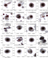 |
Fig. A.1 Morphologies of various H II regions. Each panel displays the source name and ID, along with the peak radio emission marked by cross symbols. The thick navy contours indicate the BLOBCAT regions used for the photometric measurements. They correspond to emission levels of 3 σrms for all sources, except for sources 14 and 21, where the contours correspond to 4.6 σrms and 7.6 σrms, respectively. The maroon contours represent emission levels of 5, 10, 20, 40, and 80 σrms, where the local σrms is obtained from the signal-to-noise ratio map created by BLOBCAT. Source 8 (G358.784+0.060) has a broken shell-like structure. Sources 5 (G358.599–0.060) and 15 (G358.551–0.029) show examples of the cometary morphology of H II regions. Source 19 (G358.505+0.108) is an example of multiple compact regions embedded in cometary-like diffuse gas. |
Appendix B Auxiliary data and figures
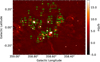 |
Fig. B.1 Sources extracted from the GLOSTAR VLA-D configuration image using BLOBCAT. They are shown as green boxes along with the assigned ID number given in Col. 1 of Tab. B.1. |
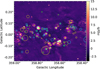 |
Fig. B.2 H II regions marked on top of the GLOSTAR VLA-D image of the target region. The magenta, cyan and gold circles represent the known, candidate and radio-quiet H II regions from the WISE H II catalog. The green crosses mark the peak flux position of the radio sources extracted from this image that are proposed to be H II regions or candidates in this work. |
Counterparts of the extracted radio sources at different wavelengths.
Catalogs used to identify counterparts from the NIR to the radio.
Classification scheme of all the radio sources toward G358.69+0.03.
Physical properties of the radio sources not classified as H II regions.
Physical properties of the H II regions.
SiO (5–4) line parameters.
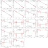 |
Fig. B.3 Spectral index plots for the H II regions. The spectral index (α), source name and ID are given in each panel. |
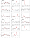 |
Fig. B.4 Spectral line (shown in red) of the SiO J=5–4 transition (rest frequency of 217.1050 GHz) for each source on the Tmb scale. The observed spectra are shown in black. The source names are presented in each panel and the plots show a −300 to +100 km s−1 velocity range. |
All Tables
All Figures
|
Fig. 1 Left: three-color infrared view of the Galactic plane on the negative longitude side, with MIPSGAL 24 μm emission in red, GLIMPSE 8 μm in green, and GLIMPSE 4.5 μm in blue. The golden box shows the SgrE star-forming complex (358.3°<l<359.3°, |b| < 0.2°; Anderson et al. 2020). Right: 1.28 GHz MeerKAT image of the target region (Heywood et al. 2022). The dashed partial circles in both panels highlight the arc-like or U-shaped morphology of G358.69+0.03. |
| In the text | |
|
Fig. 2 Left: GLOSTAR D configuration radio continuum averaged intensity map at 5.8 GHz with an angular resolution of ~18″. The dashed white circle marks the target region. Right: GLOSTAR combination image (VLA-D+Effelsberg). The dashed cyan partial circles highlight the arc-like or U-shaped morphology of G358.69+0.03. The beam sizes are shown in the lower-left corner of each panel. |
| In the text | |
|
Fig. 3 MIR colors for the 37 sources (black crosses) associated with a WISE counterpart out of the total 49 radio sources found toward G358.69+0.03 in this work. The maroon, green, and magenta circles represent the known, candidate, and radio-quiet H II regions, respectively, from the WISE Galactic H II Regions Catalog V2.3 (Anderson et al. 2014). The region above the dashed black line represents the parameter space where all the H II regions and the majority of PNe are present, as identified by Medina et al. (2019). |
| In the text | |
|
Fig. 4 Multiwavelength view of the known H II region, G358.632+0.063. First row (from left to right): Color composite images from 2MASS (Skrutskie et al. 2006), GLIMPSE, WISE, and Spitzer. The red, green, and blue colors are shown in each panel. Middle and bottom rows (from left to right and top to bottom): MIPSGAL 24 μm, Hi-GAL 70 μm, Hi-GAL 160 μm, Hi-GAL 250 μm, Hi-GAL 350 μm, Hi-GAL 500 μm, ATLASGAL 870 μm, and 5.8 GHz GLOSTAR VLA-D images of the H II region. The blue circles in the center of each panel show the peak position of radio emission. The FWHM beams of 2MASS (0.8″), GLIMPSE (2″), WISE (6″ at 12 μm), Spitzer (6″ at 24 μm), MIPSGAL (6″ at 24 μm), Hi-GAL (6″, 12″, 18″, 24″, and 35″ at 70, 160, 250, 350, and 500 μm, respectively), and ATLASGAL (19″) are indicated by the black and white circles with hatched lines shown in the lower-left corner of each panel. |
| In the text | |
|
Fig. 5 Classification of radio sources toward G358.69+0.03. The green crosses show the HII regions identified in this work. The cyan, magenta, and yellow circles mark the positions of cEGs, cPNe, and the unidentified radio (Rad) sources, respectively. The dashed white circle marks the target region. The background image shows the GLOSTAR VLA-D configuration image. The beam size is shown in the lower-left corner. |
| In the text | |
|
Fig. 6 Spectral types and Lyman continuum photon rates of the H II regions derived from the VLA-D radio continuum data. |
| In the text | |
|
Fig. 7 Left: distribution of the ATLASGAL dust continuum sources (gold markers) overlaid on top of the color composite image of G358.69+0.03. The VLA-D+Effelsberg image is shown in red and the Hi-GAL 350 and 70 μm emission maps in green and blue, respectively. The dashed white circle shows G358.69+0.03. Right: color composite image showing the VLA-D image in red and Spitzer bands of 24 and 8 μm in green and blue, respectively. The dashed white partial circles mark the arc-like or U-shaped morphology of the target region. The black circles represent the H II regions identified in this work, and the gold diamonds mark the position of ATLASGAL cold dust clumps toward G358.69+0.03. The gray, violet, and green crosses mark the positions of pre-stellar clumps, protostellar clumps, and gravitationally unbound starless Hi-GAL clumps, respectively, at a distance of 8–9 kpc toward G358.69+0.03. |
| In the text | |
|
Fig. 8 Bolometric luminosity versus mass of Hi-GAL compact sources at distances between 8 and 9 kpc toward G358.69+0.03. The clumps are color-coded by temperature. The markers with thick lines are sources with high reliability parameters taken from Elia et al. (2021). The shapes of the markers (as shown in the legend) indicate different classification categories. The low-mass regime is taken from Saraceno et al. (1996). |
| In the text | |
|
Fig. 9 Flux ratio map of Spitzer [4.5 μm]/[3.6 μm] for the target region. The black crosses show the H II regions identified in our work. The maroon, blue, and gold circles mark the known, candidate, and radio-quiet H II regions from the WISE H II catalog. |
| In the text | |
|
Fig. 10 Left: kinematics of the GC region revealed by the 12CO(3–2) longitude-velocity diagram. Right: zoomed-in view of the LV diagram of the G358.69+0.03 region (l~ −1.3° or 358.7°). Cyan stars correspond to the 57 components of the SiO emission detected toward the 15 ATLASGAL clumps listed in Table B.6. The scale bar corresponds to the assumed GC distance of 8.2 kpc. |
| In the text | |
|
Fig. 11 Sources observed with the APEX nFLASH230 receiver at a tuning frequency of 230.79 GHz (black crosses) overplotted on the inset flux ratio map of Spitzer [4.5 μm]/[3.6 μm] for the southern part of the target region, G358.69+0.03. The numbers represent the corresponding IDs of the sources given in Table B.6. The background image shows the VLA-D continuum map. |
| In the text | |
|
Fig. 12 Left: three-color map of the SgrE region. Red shows 12CO(J=3–2) emission integrated over −240 to −190 km s−1, tracing the far dust-lane component; blue shows −185 to −50 km s−1, tracing the main CMZ stream and the emission bridge observed in Fig. 10b; and green corresponds to the MeerKAT 1 GHz image, tracing the H II regions. The dashed line (AB) indicates the cut used to construct the LV diagram. Right: 12CO(J=3–2) LV diagram along the AB line, revealing a velocity bridge linking the far dust-lane gas with the CMZ stream, consistent with a site of cloud-cloud interaction. |
| In the text | |
|
Fig. 13 Schematic illustration of gas inflow into the CMZ. Left: gas streams along the near- and far-side dust lanes feed the CMZ. Sgr E is located at the intersection of the far dust lane and the CMZ orbit (adapted from Henshaw et al. 2023). Right: zoomed-in view of the collision, where the far dust lane impacts the CMZ gas, compressing material and producing an arc-like or U-shaped distribution of H II regions. |
| In the text | |
|
Fig. A.1 Morphologies of various H II regions. Each panel displays the source name and ID, along with the peak radio emission marked by cross symbols. The thick navy contours indicate the BLOBCAT regions used for the photometric measurements. They correspond to emission levels of 3 σrms for all sources, except for sources 14 and 21, where the contours correspond to 4.6 σrms and 7.6 σrms, respectively. The maroon contours represent emission levels of 5, 10, 20, 40, and 80 σrms, where the local σrms is obtained from the signal-to-noise ratio map created by BLOBCAT. Source 8 (G358.784+0.060) has a broken shell-like structure. Sources 5 (G358.599–0.060) and 15 (G358.551–0.029) show examples of the cometary morphology of H II regions. Source 19 (G358.505+0.108) is an example of multiple compact regions embedded in cometary-like diffuse gas. |
| In the text | |
|
Fig. B.1 Sources extracted from the GLOSTAR VLA-D configuration image using BLOBCAT. They are shown as green boxes along with the assigned ID number given in Col. 1 of Tab. B.1. |
| In the text | |
|
Fig. B.2 H II regions marked on top of the GLOSTAR VLA-D image of the target region. The magenta, cyan and gold circles represent the known, candidate and radio-quiet H II regions from the WISE H II catalog. The green crosses mark the peak flux position of the radio sources extracted from this image that are proposed to be H II regions or candidates in this work. |
| In the text | |
|
Fig. B.3 Spectral index plots for the H II regions. The spectral index (α), source name and ID are given in each panel. |
| In the text | |
|
Fig. B.4 Spectral line (shown in red) of the SiO J=5–4 transition (rest frequency of 217.1050 GHz) for each source on the Tmb scale. The observed spectra are shown in black. The source names are presented in each panel and the plots show a −300 to +100 km s−1 velocity range. |
| In the text | |
Current usage metrics show cumulative count of Article Views (full-text article views including HTML views, PDF and ePub downloads, according to the available data) and Abstracts Views on Vision4Press platform.
Data correspond to usage on the plateform after 2015. The current usage metrics is available 48-96 hours after online publication and is updated daily on week days.
Initial download of the metrics may take a while.