| Issue |
A&A
Volume 710, June 2026
|
|
|---|---|---|
| Article Number | A54 | |
| Number of page(s) | 11 | |
| Section | Cosmology (including clusters of galaxies) | |
| DOI | https://doi.org/10.1051/0004-6361/202558245 | |
| Published online | 28 May 2026 | |
From observations to simulations: A neural-network approach to intracluster medium kinematics
1
Max-Planck-Institut für Extraterrestrische Physik, Gießenbachstraße 1, 85748, Garching, Germany
2
Harvard-Smithsonian Center for Astrophysics, 60 Garden Street, Cambridge, MA, 02138, USA
3
Institute of Astronomy, Madingley Road, Cambridge, CB3 0HA, UK
4
Institute for Frontiers in Astronomy and Astrophysics, Beijing Normal University, Beijing, 102206, China
5
INAF – IASF Palermo, Via U. La Malfa 153, I-90146, Palermo, Italy
6
Department of Physics and Astronomy, University of Alabama in Huntsville, Huntsville, AL, 35899, USA
★ Corresponding author: This email address is being protected from spambots. You need JavaScript enabled to view it.
Received:
24
November
2025
Accepted:
25
April
2026
Abstract
We present a systematic comparison between XMM-Newton velocity maps of the Virgo, Centaurus, Ophiuchus, and A3266 clusters and synthetic velocity maps generated from the Illustris TNG-300 simulated clusters. Our goal is to constrain the physical conditions and dynamical states of the intracluster medium (ICM) through a data-driven approach. We employed a Siamese convolutional neural network (CNN) designed to identify the most analogous simulated cluster to each observed system based on the morphology of their line-of-sight velocity maps. The model learns a high-dimensional similarity metric between observations and simulated clusters, allowing us to capture subtle kinematic and structural patterns beyond traditional statistical tests. We find that the best-matching simulated halos reproduce the observed large-scale velocity gradients and local kinematic substructures, suggesting that the ICM motions in these clusters arise from a combination of gas sloshing, active galactic nucleus feedback, and minor merger activity. Our results demonstrate that deep learning provides a powerful and objective framework for connecting X-ray observations to cosmological simulations, offering new insights into the dynamical evolution of galaxy clusters and the mechanisms driving turbulence and bulk flows in the hot ICM.
Key words: galaxies: clusters: intracluster medium / galaxies: clusters: individual: ophiuchus / galaxies: clusters: individual: centaurus / galaxies: clusters: individual: virgo / galaxies: clusters: individual: A3266 / X-rays: galaxies: clusters
© The Authors 2026
 Open Access article, published by EDP Sciences, under the terms of the Creative Commons Attribution License (https://creativecommons.org/licenses/by/4.0), which permits unrestricted use, distribution, and reproduction in any medium, provided the original work is properly cited.
This article is published in open access under the Subscribe to Open model.
Open access funding provided by Max Planck Society.
1. Introduction
The intracluster medium (ICM) is a tenuous, X-ray-emitting plasma permeating galaxy clusters. Despite its extremely low density and high temperatures (∼107 − 108 K), the ICM contains several times more baryons than cluster galaxies combined (Andreon & Hurn 2010; Dai et al. 2010; Kravtsov & Borgani 2012), making it a crucial component for understanding the physics of cosmic structures. Simulations predict that the ICM should host turbulent or random motions and large-scale bulk flows arising from hierarchical merging processes (e.g., Lau et al. 2009; Vazza et al. 2011; Schmidt et al. 2017; Ha et al. 2018; Vazza et al. 2021). Additionally, sloshing motions induced by infalling substructures can generate relative bulk velocities of a few hundred kilometers per second (e.g., Ascasibar & Markevitch 2006; Ichinohe et al. 2019; Vazza et al. 2018; ZuHone et al. 2018). The central active galactic nucleus (AGN) in the brightest cluster galaxy (BCG) further contributes to ICM motions through jets and buoyantly rising relativistic plasma bubbles, potentially driving velocities of ∼100 − 500 km s−1 in surrounding gas (e.g., Brüggen et al. 2005; Heinz et al. 2010; Randall et al. 2015; Yang & Reynolds 2016; Bambic & Reynolds 2019).
Determining the kinematic properties of the ICM is therefore essential for developing a comprehensive physical picture of galaxy clusters. In this context, Sanders et al. (2020) introduced an innovative technique that leverages the instrumental X-ray lines in XMM-Newton EPIC-pn spectra to calibrate the absolute energy scale with a precision better than 100 km s−1 at the Fe–K line. Using this technique, direct measurements of ICM velocities have been obtained in several systems – including the Perseus and Coma clusters (Sanders et al. 2020), Virgo (Gatuzz et al. 2022b, 2023b), Centaurus (Gatuzz et al. 2022a, 2023d), Ophiuchus (Gatuzz et al. 2023c,a), and A3266 (Gatuzz et al. 2024, 2025) – and these results have been robustly confirmed by XRISM Resolve observations (XRISM Collaboration 2025; Fujita et al. 2025; Gatuzz et al. 2026). These studies reveal a variety of velocity structures associated with both merger-driven dynamics and AGN feedback.
The launch of the X-ray Imaging and Spectroscopy Mission (XRISM) has opened a new era of direct ICM kinematic measurements. Early Resolve observations reveal a wide range of dynamical states: relaxed systems can exhibit extremely low nonthermal support (e.g., Abell 2029 shows σv = 169 ± 10 km s−1 and a nonthermal pressure fraction of only ∼2%, XRISM Collaboration 2025). In contrast, Perseus- and Centaurus-like cool cores display measurable bulk flows consistent with sloshing, with line-of-sight velocities of 102 − 3 × 10² km s−1 detected in Centaurus (XRISM Collaboration 2025; Zhang et al. 2025). XRISM measurements in Coma reveal ordered, large-scale velocity structures and modest velocity dispersions (∼200 km s−1 in multiple fields), implying coherent bulk flows at the few 102 − 103 km s−1 level when combining several pointings (Gatuzz et al. 2026). Overall, early XRISM results indicate that cool-core regions generally exhibit lower velocity dispersions than predicted by several numerical models, providing stringent constraints on turbulent pressure support and AGN feedback. Such measurements are now essential benchmarks for calibrating and testing cosmological simulations.
Comparing the observed ICM velocity structure with simulated clusters is therefore imperative, as theoretical models predict tight correlations between velocity power spectra and thermodynamic quantities such as entropy, temperature, density, and pressure (Gaspari et al. 2014; Zhuravleva et al. 2014; Mohapatra & Sharma 2019). Deep-learning methods have emerged as powerful tools for bridging observations and simulated clusters in this context. Convolutional neural networks (CNNs) have been successfully applied to tasks such as galaxy morphology classification, feature extraction in large surveys, and inference of physical properties from real and simulated data (Huertas-Company et al. 2015; Domínguez Sánchez et al. 2018; Pearson 2019). Among these architectures, Siamese CNNs – networks designed to learn a similarity metric between inputs – enable robust comparison even in limited-data scenarios. Brunel et al. (2019) employed a Siamese CNN for supernova classification using sparse light curves, and Zhang et al. (2022) applied a similar architecture to galaxy morphology classification with few labeled examples, demonstrating the general utility of deep metric learning for astrophysical inference.
Here, we present a systematic comparison between the velocity maps obtained for the Virgo, Centaurus, and Ophiuchus clusters and magnetohydrodynamic simulations, using a Siamese CNN to infer the physical conditions of the ICM. While previous deep-learning efforts have compared other ICM observables (e.g., X-ray surface brightness or temperature) across simulated clusters and observations, the velocity field remains the most complex and least constrained. We therefore focus this initial work exclusively on the kinematic structure to evaluate the performance of the Siamese framework in this challenging domain. This paper is organized as follows. Section 2 describes the XMM-Newton observations used in the analysis. Section 3 presents the magnetohydrodynamic simulations employed. Section 4 outlines the Siamese CNN methodology. Section 5 reports the results of the CNN-based similarity analysis. Section 6 discusses and interprets the best-matching simulated velocity maps. Finally, Sect. 8 summarizes our conclusions. Throughout this work, we adopt a Λ Cold Dark Matter (CDM) cosmology with Ωm = 0.3089, ΩΛ = 0.6911, and H0 = 67.74 km s−1 Mpc−1.
2. ICM velocity maps: XMM-Newton observations
For this study, we used velocity maps of the Virgo (Gatuzz et al. 2022b, 2023b), Centaurus (Gatuzz et al. 2022a, 2023d), Ophiuchus (Gatuzz et al. 2023c,e), and A3266 (Gatuzz et al. 2024, 2025) clusters. Here, we summarize the procedure used to generate the velocity maps. The XMM-Newton EPIC data were reduced with SAS (version 19.1.0) using epchain, selecting single-pixel events (PATTERN==0), filtering soft-proton flares (threshold 1.0 cts/s), and removing bad pixels and charge-coupled device (CCD) edges (FLAG==0). Point sources, including central AGNs, were detected with edetect_chain (detection likelihood det_ml > 10) and masked. Following Sanders et al. (2020) and Gatuzz et al. (2022b,a), velocity maps were constructed from adaptive elliptical regions (2:1 axis ratio, tangentially oriented) sized to contain ∼500−750 Fe-K counts, sampled on a 0.25 arcmin grid. Spectra from all exposures within each bin were combined and fitted in XSPEC (version 12.11.1) using the cash statistic. The ICM emission was modeled with the apec model (Foster et al. 2019), except in Centaurus where a lognorm model accounted for its multi-temperature structure; Galactic absorption was included via tbabs (Wilms et al. 2000). Free parameters included redshift, temperature, metallicity, normalization (and log σ for the lognorm model), and instrumental background lines (Cu-Kα, Cu-Kβ, Ni-Kα, and Zn-Kα) were explicitly added. This procedure yields a line-of-sight velocity precision better than 100 km/s at the Fe-K line (Sanders et al. 2020).
The resulting velocity maps reveal complex and diverse kinematic structures in the ICM across the analyzed clusters. In the Virgo cluster, the velocity field shows signatures consistent with both AGN-driven outflows and gas sloshing within the core (Gatuzz et al. 2022b). For the Centaurus cluster, a clear radial velocity gradient extends to large radii, with distinct variations coincident with cold fronts (Gatuzz et al. 2022a). In Ophiuchus, a prominent redshifted–blueshifted interface is detected ∼150 kpc east of the cluster center, coinciding with X-ray surface brightness discontinuities (Gatuzz et al. 2023c). In A3266, the hot gas exhibits a globally redshifted systemic velocity relative to the cluster mean across the field of view (Gatuzz et al. 2024). Overall, most clusters lack the characteristic spiral or symmetric redshift–blueshift patterns associated with sloshing, suggesting that the line of sight is approximately perpendicular to the sloshing plane (ZuHone et al. 2016). Localized high-velocity regions may instead be linked to AGN feedback or merger-induced motions, though weak Fe-K emission in these areas increases velocity uncertainties (Gatuzz et al. 2023c).
3. IllustrisTNG
The IllustrisTNG project is a suite of state-of-the-art cosmological magnetohydrodynamic simulations that improve upon the original Illustris simulated clusters by incorporating more refined physical models and larger cosmological volumes (Springel et al. 2018; Pillepich et al. 2018; Naiman et al. 2018; Marinacci et al. 2018; Nelson et al. 2018, 2019). Using the moving-mesh code AREPO (Springel 2010), IllustrisTNG simulates various physical processes including radiative cooling, star formation, supernova and AGN feedback, as well as chemical enrichment. The TNG simulations have been widely applied to study cluster physics, including cool core formation (Barnes et al. 2018), black hole feedback (Weinberger et al. 2018), and ram-pressure stripping in dense environments (Yun et al. 2019). The suite comprises TNG50, TNG100, and TNG300, with box sizes of 51.7, 110.7, and 302.6 Mpc, respectively. All simulations adopt a ΛCDM cosmology consistent with Planck Collaboration XIII (2016) and evolve from a redshift of z = 127 to z = 0. Structures are identified using the friends-of-friends (FoFs) algorithm and the SUBFIND algorithm (Springel et al. 2001; Dolag et al. 2009), and galaxies are defined as subhalos with nonzero stellar mass.
We used TNG300, which provides the largest cosmological volume and a statistically significant population of massive galaxy clusters. TNG300 contains over 280 halos with log(M200/M⊙) > 14 and several with log(M200/M⊙) > 15 (Sohn et al. 2017), with 2 × 25003 resolution elements (dark matter particles and gas cells), a baryon mass resolution of mbaryon ∼ 1.1 × 10⁷ M⊙, and dark matter particle mass mDM ∼ 5.9 × 10⁷ M⊙. Galaxy formation histories were traced using SubLink and LHaloTree merger trees (Rodriguez-Gomez et al. 2015; Springel et al. 2005), following the main progenitor branch at each timestep. The gravitational softening length for the stellar component is ∼1 kpc at z = 0, and the minimum gas cell size can reach ≲1 kpc, enabling detailed modeling of ICM thermodynamics and kinematics. From this sample, we selected 40 galaxy clusters at z = 0 with masses up to ∼1015 M⊙, consistent with the observed clusters of interest.
Synthetic observations were generated to enable direct comparison with our XMM-Newton maps. Following ZuHone et al. (2024), we used the pyXSIM package (ZuHone & Hallman 2016) to produce X-ray emissivity maps. Gas cells with T > 3 × 10⁵ K were included, while cooler and denser star-forming phases were excluded by applying a density cut of ρ < 5 × 10⁻²⁵ g cm−3. X-ray emissivities (line plus continuum) in the 0.1−10 keV band were computed assuming collisional ionization equilibrium with apec (Foster et al. 2019), and projected maps of surface brightness and bulk velocity were constructed from the emissivity-weighted quantities. To define the reference velocity frame, the systemic velocity of the BCG was estimated from the halo stellar component. The stellar density peak was located, and the mean velocity of stellar particles within an aperture of 20−30 kpc was computed, excluding satellites and intracluster light. This velocity vector was adopted as the systemic frame, and all gas and particle velocities were re-centered accordingly before generating synthetic velocity maps in total.
To explore projection effects beyond the standard Cartesian axes (X, Y, Z), we generated additional synthetic observations along 100 distinct lines of sight for each of the 40 halos. These orientations were defined by polar and azimuthal angles θ ∈ [5° ,85° ] and ϕ ∈ [0° ,175° ] in 10° intervals. The directional cosines for each line of sight were computed as
 (1)
(1)
 (2)
(2)
 (3)
(3)
These unit vectors enabled the construction of projected maps from a broad range of viewing angles. The final comparison sample consists of 4120 synthetic velocity maps.
4. Deep learning approach for velocity map matching
Traditional statistical approaches – such as χ2 or likelihood-based tests – directly compare binned quantities or predefined features. In contrast, a machine learning framework can learn a complex, high-dimensional representation of the data, capturing subtle morphological and kinematic variations that may be overlooked by simpler statistical metrics. In this work, we adopted a deep learning approach based on velocity map data to identify the simulated cluster that most closely resembles each XMM-Newton observation. Specifically, we employed a Siamese CNN consisting of two identical branches that share the same architecture and weights, allowing the model to learn a data-driven similarity metric between input maps.
Figure 1 illustrates the CNN architecture used in our analysis. The network acts as a feature extractor, transforming raw 2D pixel data into a compact numerical vector in a high-dimensional latent space. It consists of multiple convolutional layers that progressively extract hierarchical spatial and kinematic features, with max-pooling layers reducing spatial dimensionality while retaining salient features. After the final convolutional block, a flattening layer converts the feature maps into a 1D vector, which is then passed through fully connected (dense) layers to refine high-level representations. The final dense layer outputs the embedding vector–a concise numerical representation encapsulating the essential kinematic characteristics of the input velocity map. This CNN encoder serves as the backbone of the Siamese network. To ensure fair comparison, the XMM-Newton velocity maps were re-binned to match the spatial resolution and physical scale of the simulated clusters, using linear interpolation to preserve data integrity.
 |
Fig. 1. Diagram of the CNN architecture used in our analysis. The network processes 128 × 128 × 1 input velocity maps through a series of convolution and max-pooling layers to extract hierarchical features. The resulting feature map is flattened and passed through a fully connected dense layer of 512 units, culminating in a 128D embedding vector that provides a compact, discriminative representation of the cluster kinematics. |
Figure 2 presents the Siamese CNN training process. The network is trained using the triplet loss function (Schroff et al. 2015), which operates on three input images: an anchor (A), a positive (P), and a negative (N). The loss function is defined as
 (4)
(4)
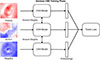 |
Fig. 2. Diagram of the Siamese CNN training phase. During training, triplets of velocity maps are passed through identical CNN encoders with shared weights. Each triplet consists of a reference (Anchor), a matched projection from the same simulated cluster (Positive), and a mismatched projection from a different simulated cluster (Negative). The network learns to produce similar embeddings for the Anchor–Positive pairs and dissimilar embeddings for the Anchor–Negative pairs by minimizing the triplet loss. This process teaches the model to recognize the underlying kinematic structure of clusters, independent of projection and resolution differences. |
where f denotes the CNN embedding function and α is the margin parameter. This loss minimizes the distance between the anchor and positive embeddings while maximizing the distance between the anchor and negative embeddings beyond the margin. During training, network weights were updated via back-propagation, effectively organizing the embedding space such that similar velocity maps cluster together and dissimilar maps are pushed apart. Specifically, each triplet was constructed by selecting a reference velocity map (Anchor), a second projection of the same simulated cluster taken from a different line of sight (Positive), and a projection from an entirely different simulated cluster (Negative). By enforcing similarity between different viewpoints of the same physical system, the network was trained to ignore orientation-dependent morphological variations and instead extract latent kinematic features that characterize the underlying physical state of the halo. While different projections of a disturbed system may not always resemble each other visually, the triplet loss effectively forces the model to identify the deeper, invariant physical signatures common to that specific simulated cluster.
To mitigate overfitting and ensure unbiased performance, the simulated velocity maps were divided into independent training and validation sets. To ensure the learned representation is invariant to orientation in the focal plane, we utilized data augmentation during the training process, subjecting each input map to random 90° rotations and performing horizontal and vertical flips. The training set comprised 10% of the total simulated clusters. Tests confirmed that increasing this fraction yielded consistent results, demonstrating the robustness of this method. As additional validation, the network was trained on artificially generated datasets containing the XMM-Newton observation, perturbed versions, and purely random maps. Perturbed images were produced by applying pixel shifts and rotations, while random maps were drawn from a uniform pixel-value distribution. The network correctly identified the unperturbed observation as the closest match, confirming that it learned physically meaningful kinematic representations.
Once training was complete, the matching phase was initiated (Fig. 3). In this stage, the trained Siamese CNN branch serves as a fixed feature extractor with frozen weights. The observed XMM-Newton velocity map was first passed through the network to generate its unique embedding vector f(O). Subsequently, each TNG300 simulated cluster map was processed through the same network to obtain its corresponding embedding f(Sj). To ensure consistency, all simulated cluster maps were resampled to match the spatial resolution of the observational data. The similarity between the observation and each simulated cluster was quantified via the Euclidean distance in the learned latent space:
![Mathematical equation: $$ \begin{aligned} \mathrm{D}(O, S_j) = \Vert f(O) - f(S_j)\Vert _2 = \sqrt{\sum _{k = 1}^{N_{\rm emb}} \left[f(O)_k - f(S_j)_k\right]^2}, \end{aligned} $$](/articles/aa/full_html/2026/06/aa58245-25/aa58245-25-eq5.gif) (5)
(5)
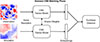 |
Fig. 3. Diagram of the Siamese CNN matching phase. During matching, the trained Siamese CNN compares each observed XMM-Newton velocity map to the full library of simulated velocity maps. Both the observed map and each simulated cluster are passed through the shared-weight CNN encoder to generate corresponding embedding vectors. Similarity between the observation and a given simulated cluster is quantified by the distance between their embeddings in the learned latent space. Simulated clusters with the smallest embedding distance are identified as the closest kinematic matches, enabling a quantitative, model-driven comparison between observed cluster dynamics and the cosmological simulations. |
where Nemb represents the dimensionality of the embedding vector. The embedding function f maps the complex kinematic features onto a high-dimensional manifold where the vectors are constrained to a unit hypersphere (or “normalized to the range [0, 1]”). By operating within this normalized latent space, the reported Euclidean distances represent the relative degree of morphological and kinematic dissimilarity between clusters. A distance value approaching zero (e.g., D ≈ 0.002) indicates a near-exact convergence of kinematic patterns within the scale of the simulated clusters sample. The simulated cluster that minimizes this distance is identified as the best match, providing a quantitative, data-driven framework for linking simulated halos to observed ICM velocity structures.
5. CNN-based similarity matching results
5.1. Hyperparameter tuning and model optimization
The performance of the Siamese CNN was optimized through a rigorous hyperparameter tuning process. Table 1 lists the parameters governing the model architecture and training dynamics, alongside their optimized values. To efficiently constrain these hyperparameters, a random search approach was employed. This method systematically explores various parameter combinations within predefined ranges, offering a more efficient discovery of promising regions in the hyperparameter space compared to a fixed grid search. During this process, the Adam optimizer was utilized for weight updates, with the learning rate itself treated as a tunable hyperparameter to ensure optimal convergence for the velocity map features. During each trial, a new CNN branch and triplet model were initialized and trained. The primary objective was to identify the set of hyperparameters that yielded the lowest triplet loss on the training data. The weights of the best-performing model were subsequently saved and used for the final embedding generation and similarity matching. This systematic optimization, supported by an automated search framework, ensures a robust network configuration that effectively captures the underlying patterns in the velocity maps.
Optimized hyperparameters controlling the Siamese CNN architecture.
5.2. Embedding space visualization and analysis
To visually inspect the relationships between observed and simulated velocity maps, we employed t-distributed stochastic neighbor embedding (t-SNE) to reduce the high-dimensional CNN embeddings to a 2D space. The results are shown in Fig. 4. In this space, similar data points are represented by nearby points, while dissimilar points are farther apart. Notably, the simulated clusters are not uniformly scattered; the resulting structures (e.g., filaments and curves) reflect continuous evolutionary sequences and physical gradients captured by the CNN. Each panel corresponds to a different galaxy cluster, showing the observed velocity map (red point) and its best match from the TNG300 sample based on Euclidean distance (blue point). These plots indicate that the TNG300 sample contains highly analogous objects with velocity structures closely resembling the observed ones. It is important to note that while t-SNE preserves the local neighborhood structure, the nonlinear, nonmetric nature of the projection means that 2D distances do not precisely reflect the true high-dimensional Euclidean distances used for similarity ranking.
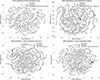 |
Fig. 4. t-SNE plots comparing the observed velocity maps of four galaxy clusters to the TNG simulation library. While all embeddings were generated using a single trained Siamese CNN, we present independent t-SNE projections for each source to clearly visualize the specific matches within the broader simulated distribution. Points represent the relative similarity of velocity maps in the latent space, with proximity indicating a closer kinematic match. The nonuniform distribution of the TNG-simulated clusters reflects underlying physical gradients and evolutionary sequences learned by the network. The axes are arbitrary, and quantitative similarity rankings (blue) are calculated based on Euclidean distances in the original high-dimensional embedding space rather than these 2D stochastic projections. |
To identify not only the single best match but also simulated clusters close in embedded features, we implemented a relative threshold. We first determined the Euclidean distance dbest of the single best-matching simulated cluster to the XMM-Newton velocity map. A simulated cluster was classified as a “very close” match if its distance dsim satisfied
 (6)
(6)
where p is a defined percentage threshold (e.g., p = 0.20 for a 20% threshold). This approach ensures that the search for similar simulated clusters is contextual and focuses around the best-fitting halo. Applying this conservative threshold, we find that the “very close” matches for each cluster correspond to the same halo from the simulation suite, differing only by their 3D orientation. This result validates the Siamese CNN’s capability, demonstrating that the embedding space successfully captures the intrinsic structure of a halo and correctly clusters rotational variants as highly similar rather than treating them as distinct entities.
6. Kinematic analysis of the ICM: Observations versus simulated clusters
Table 2 lists the best-matching halos identified for each observed cluster, including their projected coordinates (x, y, z), the Euclidean distance from the Siamese CNN comparison, and the corresponding total stellar mass, gas mass, and star formation rate (SFR) within R200. Figure 5 presents the line of sights (LOS) velocity maps for these best-matching systems. In the following subsections, we compare the baryonic properties and velocity structures of the best-matching TNG300 halos with those of the corresponding XMM-Newton observations.
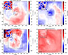 |
Fig. 5. Best-matching velocity maps from the TNG300 simulated clusters obtained with the Siamese CNN analysis for the XMM-Newton observations. The zoom-in panel shows the XMM-Newton data for a region centered on the physical origin (0, 0 kpc) of the simulated cluster. All simulated maps are presented at a fixed physical scale to maintain consistency across the sample. The apparent difference in coverage between the panels (e.g., A3266 vs. Virgo) is a result of the different angular sizes and distances of the observed clusters. Showing the full simulated extent provides crucial context for the large-scale dynamics and merger history that drive the observed core kinematics, offering insights into the broader physical environment of the matched systems. These figures illustrate kinematic similarity based on the CNN-learned metric, rather than pixel-wise visual resemblance. |
Summary of TNG300 halo properties from the best matches between XMM-Newton observations and simulated clusters.
6.1. The Virgo galaxy cluster
The Virgo Cluster, centered on M87, exhibits complex ICM kinematics shaped by both merger activity and AGN feedback. The Siamese CNN identified halo #14 in TNG300 as the best kinematic match to the observed LOS velocity field, with projected coordinates (x, y, z) = (0.41, −0.91, 0.41) (Fig. 5, top left). The best-matching simulated clusters reproduces the main baryonic components of Virgo with good fidelity. At R200, the simulated gas mass,  , falls comfortably within the observational range of (0.4 − 1.7)×1014 M⊙ (Nulsen & Bohringer 1995; Simionescu et al. 2010; McCall et al. 2024), indicating that the TNG300 model accurately captures the global thermodynamic state and gas extent of the cluster. The stellar mass,
  , lies slightly below the lower limit of the observed interval (5.0 − 20)×1012 M⊙ (Ferrarese et al. 2012, 2016; Sánchez-Janssen et al. 2019; Morgan et al. 2025), suggesting a mild underestimation of star formation efficiency or past merger-driven buildup in the model. The total SFR of SFRsim = 4.6 M⊙ yr−1 also resides near the lower bound of the observed range (5 − 20 M⊙ yr−1) (Cortese et al. 2012; Gavazzi et al. 2012; Boselli et al. 2023; Edler et al. 2024), consistent with Virgo’s quiescent nature. We note, however, that due to the limited training size and reference sets available for this study, these comparative inferences should be viewed as illustrative and interpreted with caution rather than as a definitive assessment of systemic discrepancies in the TNG300 physics.
Both the simulated cluster and the XMM-Newton data show a large-scale velocity gradient across the cluster core, indicative of gas sloshing triggered by a minor merger (Gatuzz et al. 2022b). In the observed map, gas within r < 30 kpc is blueshifted relative to M87, while gas at larger radii is redshifted–a pattern reproduced by the best-matching TNG300 halo. At smaller scales, the XMM-Newton data show localized, oppositely directed velocity features (vE ≈ +1200 km/s, vW ≈ −1500 km/s) associated with AGN-driven gas outflows (Gatuzz et al. 2022b). While the simulated cluster captures the broad east-west velocity asymmetry, it yields smoother gradients, likely reflecting the limited spatial resolution of the AGN feedback model in TNG300, which lacks explicit jet evolution or resolved bubble dynamics (Owen et al. 2000; Forman et al. 2007). Furthermore, an inspection of the mass assembly history of the best-matched TNG halo confirms a steady growth profile without recent major merger events, consistent with the relatively relaxed kinematic state observed in the Virgo velocity maps.
6.2. The Centaurus galaxy cluster
The Centaurus Cluster is a cool-core system exhibiting both AGN feedback and complex gas dynamics. The Siamese CNN identified halo #35 from TNG300 as the closest kinematic analog, with coordinates (x, y, z) = (0.09, −0.39, 0.09) (Fig. 5, top right). At R200, the simulated gas mass,  , lies close to the lower edge of the observed range (6.0 − 15)×1013 M⊙ (Sanders et al. 2016; Walker et al. 2013; Veronica et al. 2025), suggesting that the dominant baryonic component is well modeled. In contrast, the stellar mass is significantly underestimated (
 vs. observed > 1.0 × 10¹³ M⊙), likely reflecting either an underproduction of the BCG and intracluster light or overly strong quenching in massive halos (Misgeld et al. 2009; Saviane & Jerjen 2007; Liu et al. 2012). Similarly, the total SFR, SFRsim = 1.0 M⊙ yr−1, is lower than the observed 5 − 15 M⊙ yr−1 range (Mittal et al. 2011; Fabian et al. 2016), consistent with the excessive suppression of residual cooling and star formation in the TNG model. We note, however, that due to the limited training size and reference sets available for this study, these comparative inferences should be viewed as illustrative and interpreted with caution rather than as a definitive assessment of systemic discrepancies in the TNG300 physics.
The XMM-Newton velocity map reveals a prominent blueshifted region southwest of the core, reaching ∼900 km/s (Gatuzz et al. 2022a; XRISM Collaboration 2025), with no clear spiral pattern characteristic of large-scale sloshing. The best-matching TNG300 halo reproduces this SW blueshift feature and the absence of a strong sloshing signature, implying that the observed “Centaurus wind” could result from bulk ICM motion or weak sloshing along the line of sight, rather than direct AGN jet feedback. Small-scale redshifted patches observed near the core are less pronounced in the simulated cluster, possibly due to the limited kinematic resolution or observational noise. The absence of recent major mergers in the assembly history of the identified TNG match reinforces the interpretation of Centaurus as a system whose kinematic features are driven by internal processes rather than large-scale structural collisions.
6.3. The Ophiuchus galaxy cluster
The Ophiuchus Cluster is an extremely massive, X-ray luminous system exhibiting disturbed kinematics consistent with a recent or ongoing merger. The Siamese CNN selected halo #2 from TNG300 as the best match, with coordinates (x, y, z) = (0.33, 0.08, 0.33) (Fig. 5, bottom left). The simulated baryonic properties show excellent agreement with observations. The stellar mass within R200,  , aligns with the measured
  (Durret et al. 2015). The gas mass,
  , also agrees with the observed range of (1 − 2)×1014 M⊙ well (Liu et al. 2020; Gatuzz et al. 2023c,e). The simulated SFR, SFRsim = 1.33 M⊙ yr−1, slightly exceeds the observational upper limit of < 10 M⊙ yr−1 (Durret et al. 2015), suggesting a modest overprediction of residual star formation in an otherwise quenched cool-core cluster. We note, however, that due to the limited training size and reference sets available for this study, these comparative inferences should be viewed as illustrative and interpreted with caution rather than as a definitive assessment of systemic discrepancies in the TNG300 physics.
The observed LOS velocity field shows strong radial asymmetries, with a blueshifted core and a redshifted envelope, separated by a sharp velocity discontinuity Δv ∼ 2500 km/s ∼150 kpc east of the center (Gatuzz et al. 2023c; Fujita et al. 2025). The best-matching TNG halo reproduces the overall velocity structure – including the asymmetric east-side discontinuity and large-scale velocity amplitudes (> 1000 km/s) – supporting the interpretation of Ophiuchus as a major off-axis merger. However, the simulated transition between the blue- and redshifted regions is smoother, consistent with the finite resolution and dissipative numerical treatment of shocks in the simulated cluster. Nonetheless, the asymmetry between the eastern and western sides of the cluster is well reproduced, indicating that the model captures the merger geometry and resulting large-scale gas dynamics. Independent validation from the TNG merger trees reveals that the best-matched halo for Ophiuchus underwent a major mass-accretion event at z ∼ 0.32, providing physical support for the major off-axis merger scenario identified by our kinematic analysis.
6.4. The A3266 galaxy cluster
Abell 3266 is a dynamically young system exhibiting large-scale bulk motions and substructures consistent with an ongoing major merger (Gatuzz et al. 2024). The Siamese CNN identified halo #57 from TNG300 as the best kinematic match, with projected coordinates (x, y, z) = (0.0, 0.24, 0.0) (Fig. 5, bottom right). The best-matching halo shows baryonic properties broadly consistent with observations. The stellar mass,  , lies within the wide observational range (0.2 − 12)×1012 M⊙ (Gonzalez et al. 2013; Babyk et al. 2014), while the gas mass,
  , sits at the lower end of the measured (0.3 − 1.9)×1014 M⊙ range (De Grandi & Molendi 1999; Henriksen et al. 2000; Sanders et al. 2022). The simulated total SFR, SFRsim = 5.5 M⊙ yr−1, remains below the observational upper limit of SFRtot < 10 M⊙ yr−1 (Quintana et al. 1996; Henriksen & Dusek 2021), suggesting a realistic, moderate level of star formation possibly sustained by merger-induced gas compression (Henriksen & Dusek 2021). We note, however, that due to the limited training size and reference sets available for this study, these comparative inferences should be viewed as illustrative and interpreted with caution rather than as a definitive assessment of systemic discrepancies in the TNG300 physics.
The observed XMM-Newton velocity field shows redshifted gas motions across the entire field, increasing from ∼300 km/s in the northwest to ∼800 km/s in the southeast, consistent with merger-driven bulk motion (Gatuzz et al. 2024). The TNG300 simulated cluster reproduces this large-scale redshifted gradient and the characteristic C-shaped velocity structure visible in the data, confirming that the observed ICM dynamics likely result from the projected motion of subcluster components during a major merger event (Liu et al. 2015, 2016; Ota & Yoshida 2016; Liu et al. 2018). The selection of a TNG halo with a documented major merger at redshift z ∼ 1.4 as the best kinematic match for A3266 confirms that our framework effectively identifies the complex velocity structures associated with significant cluster assembly events.
7. Caveats and limitations
The main caveats in our analysis are as follows:
-
Full XMM-Newton response modeling was not included in generating the simulated maps due to computational cost and the complexity of multiple pointings. Instead, we directly compared the physical velocity maps, a simplification that enables efficient testing of the CNN framework. Future work will explore incorporating more realistic mock observations.
-
Our machine learning approach here focuses on the line-of-sight velocity maps. Future work will aim to incorporate a broader range of robust physical observables (including X-ray surface brightness and more accurately constrained temperature and metallicity maps) into the Siamese CNN method, provided such reliable maps can be consistently extracted from the data.
-
The statistical robustness of our comparative inferences is constrained by the limited training size and reference sets. With a sample of 40 TNG300 clusters used for the final comparison, the identified counterparts should be viewed as illustrative case studies for kinematic similarity. Consequently, physical interpretations of discrepancies in star formation efficiency or mass buildup between the specific simulated matches and observations should be treated as preliminary rather than a definitive assessment of systemic model performance.
8. Conclusions
In this work, we developed a deep-learning framework based on a CNN to quantify the morphological similarity between observed and simulated ICM velocity maps. This approach enables a fully data-driven, nonparametric comparison between XMM-Newton observations and TNG300 simulated clusters, providing a robust method for linking observed gas kinematics to cosmological models. The Siamese CNN was trained using a triplet-loss objective to construct a discriminative embedding space in which morphologically similar velocity structures lie in close proximity. The resulting embeddings successfully cluster different projections of the same simulated halo, demonstrating that the model learns orientation-invariant kinematic features and effectively mitigates projection effects.
A t-SNE visualization of the learned CNN embeddings further shows that each observed cluster is closely associated with a simulated halo in this feature space, indicating that the model captures physically meaningful similarities in ICM velocity morphology. The best-matching halos identified for the Virgo, Centaurus, Ophiuchus, and A3266 clusters exhibit velocity structures consistent with those observed by XMM-Newton, including coherent large-scale gradients and localized substructures linked to AGN feedback or merger-induced motions. In agreement with expectations from hydrodynamical simulations, these results suggest that the ICM dynamics in the analyzed systems are shaped by a combination of gas sloshing, AGN-driven outflows, and minor merger activity.
Quantitative comparisons between the observed and simulated baryonic components reveal overall consistency across the sample. The best-matching TNG300 halos reproduce the observed gas masses within uncertainties, slightly underpredict the stellar masses, and generally yield SFRs near or below observed values. In the TNG300 framework, AGN feedback becomes increasingly important within radii of approximately r ≲ 50 − 100 kpc, where it begins to compete with or exceed the dynamical impact of sloshing and minor mergers; outside this region, sloshing-induced motions tend to dominate. The agreement found here supports the global validity of the TNG300 feedback model while also leaving room for refinement. If future work incorporating additional cluster properties (e.g., thermodynamic profiles, radial and azimuthal velocity statistics, and metallicity structure) confirms the systematic trends identified in this study, current assumptions regarding AGN feedback efficiency and star-formation suppression in simulated clusters may require revision.
Overall, the framework presented here provides a scalable and reproducible pathway for connecting high-resolution X-ray observations with large-volume cosmological simulations. While the current study focuses on the TNG300 suite, ongoing and future work will expand this comparison to include a broader range of high-resolution simulations, such as TNG-Cluster, Magneticum, and EAGLE, to better capture fine-scale AGN-driven features and increase statistical robustness. It establishes a foundation for future studies with next-generation X-ray observatories such as Athena, which will deliver unprecedented velocity precision and enable direct tests of ICM kinematics and feedback physics across cosmic time.
Acknowledgments
This work was supported by the Deutsche Zentrum für Luft- und Raumfahrt (DLR) under the Verbundforschung programme (Kartierung der Baryongeschwindigkeit in Galaxienhaufen). This work is based on observations obtained with XMM-Newton, an ESA science mission with instruments and contributions directly funded by ESA Member States and NASA. This research was carried out on the High Performance Computing resources of the cobra cluster at the Max Planck Computing and Data Facility (MPCDF) in Garching operated by the Max Planck Society (MPG). The full simulation outputs, including snapshot data and group catalogs, are publicly available via the ILLUSTRISTNG data release portal (https://www.tng-project.org).
References
- Andreon, S., & Hurn, M. A. 2010, MNRAS, 404, 1922 [NASA ADS] [Google Scholar]
- Ascasibar, Y., & Markevitch, M. 2006, ApJ, 650, 102 [Google Scholar]
- Babyk, I. V., Del Popolo, A., & Vavilova, I. B. 2014, Astron. Rep., 58, 587 [Google Scholar]
- Bambic, C. J., & Reynolds, C. S. 2019, ApJ, 886, 78 [NASA ADS] [CrossRef] [Google Scholar]
- Barnes, D. J., Vogelsberger, M., Kannan, R., et al. 2018, MNRAS, 481, 1809 [Google Scholar]
- Boselli, A., Fossati, M., Côté, P., et al. 2023, A&A, 675, A123 [NASA ADS] [CrossRef] [EDP Sciences] [Google Scholar]
- Brüggen, M., Ruszkowski, M., & Hallman, E. 2005, ApJ, 630, 740 [Google Scholar]
- Brunel, A., Pasquet, J., Pasquet, J., et al. 2019, arXiv e-prints [arXiv:1901.00461] [Google Scholar]
- Cortese, L., Ciesla, L., Boselli, A., et al. 2012, A&A, 540, A52 [NASA ADS] [CrossRef] [EDP Sciences] [Google Scholar]
- Dai, X., Bregman, J. N., Kochanek, C. S., & Rasia, E. 2010, ApJ, 719, 119 [NASA ADS] [CrossRef] [Google Scholar]
- De Grandi, S., & Molendi, S. 1999, ApJ, 527, L25 [NASA ADS] [CrossRef] [Google Scholar]
- Dolag, K., Borgani, S., Murante, G., & Springel, V. 2009, MNRAS, 399, 497 [Google Scholar]
- Domínguez Sánchez, H., Huertas-Company, M., Bernardi, M., Tuccillo, D., & Fischer, J. L. 2018, MNRAS, 476, 3661 [Google Scholar]
- Durret, F., Wakamatsu, K., Nagayama, T., Adami, C., & Biviano, A. 2015, A&A, 583, A124 [NASA ADS] [CrossRef] [EDP Sciences] [Google Scholar]
- Edler, H. W., Roberts, I. D., Boselli, A., et al. 2024, A&A, 683, A149 [NASA ADS] [CrossRef] [EDP Sciences] [Google Scholar]
- Fabian, A. C., Walker, S. A., Russell, H. R., et al. 2016, MNRAS, 461, 922 [NASA ADS] [CrossRef] [Google Scholar]
- Ferrarese, L., Côté, P., Cuillandre, J.-C., et al. 2012, ApJS, 200, 4 [Google Scholar]
- Ferrarese, L., Côté, P., Sánchez-Janssen, R., et al. 2016, ApJ, 824, 10 [NASA ADS] [CrossRef] [Google Scholar]
- Forman, W., Jones, C., Churazov, E., et al. 2007, ApJ, 665, 1057 [NASA ADS] [CrossRef] [Google Scholar]
- Foster, A., Smith, R., & Brickhouse, N. S. 2019, Am. Astron. Soc. Meet. Abstr., 233, 251.05 [NASA ADS] [Google Scholar]
- Fujita, Y., Fukushima, K., Sato, K., Fukazawa, Y., & Kondo, M. 2025, PASJ, 77, S270 [Google Scholar]
- Gaspari, M., Churazov, E., Nagai, D., Lau, E. T., & Zhuravleva, I. 2014, A&A, 569, A67 [NASA ADS] [CrossRef] [EDP Sciences] [Google Scholar]
- Gatuzz, E., Sanders, J. S., Canning, R., et al. 2022a, MNRAS, 513, 1932 [NASA ADS] [CrossRef] [Google Scholar]
- Gatuzz, E., Sanders, J. S., Dennerl, K., et al. 2022b, MNRAS, 511, 4511 [NASA ADS] [CrossRef] [Google Scholar]
- Gatuzz, E., Mohapatra, R., Federrath, C., et al. 2023a, MNRAS, 524, 2945 [NASA ADS] [CrossRef] [Google Scholar]
- Gatuzz, E., Sanders, J. S., Dennerl, K., et al. 2023b, MNRAS, 520, 4793 [NASA ADS] [CrossRef] [Google Scholar]
- Gatuzz, E., Sanders, J. S., Dennerl, K., et al. 2023c, MNRAS, 522, 2325 [NASA ADS] [CrossRef] [Google Scholar]
- Gatuzz, E., Sanders, J. S., Dennerl, K., et al. 2023d, MNRAS, 525, 6394 [NASA ADS] [CrossRef] [Google Scholar]
- Gatuzz, E., Sanders, J. S., Dennerl, K., et al. 2023e, MNRAS, 526, 396 [NASA ADS] [CrossRef] [Google Scholar]
- Gatuzz, E., Sanders, J., Liu, A., et al. 2024, A&A, 692, A108 [NASA ADS] [CrossRef] [EDP Sciences] [Google Scholar]
- Gatuzz, E., Sanders, J., Liu, A., et al. 2025, A&A, 698, A94 [NASA ADS] [CrossRef] [EDP Sciences] [Google Scholar]
- Gatuzz, E., Sanders, J., Liu, A., et al. 2026, A&A, 706, L21 [NASA ADS] [CrossRef] [EDP Sciences] [Google Scholar]
- Gavazzi, G., Fumagalli, M., Galardo, V., et al. 2012, A&A, 545, A16 [NASA ADS] [CrossRef] [EDP Sciences] [Google Scholar]
- Gonzalez, A. H., Sivanandam, S., Zabludoff, A. I., & Zaritsky, D. 2013, ApJ, 778, 14 [Google Scholar]
- Ha, J.-H., Ryu, D., & Kang, H. 2018, ApJ, 857, 26 [NASA ADS] [CrossRef] [Google Scholar]
- Heinz, S., Brüggen, M., & Morsony, B. 2010, ApJ, 708, 462 [Google Scholar]
- Henriksen, M. J., & Dusek, S. 2021, Int. J. Astron. Astrophys., 11, 95 [Google Scholar]
- Henriksen, M., Donnelly, R. H., & Davis, D. S. 2000, ApJ, 529, 692 [NASA ADS] [CrossRef] [Google Scholar]
- Huertas-Company, M., Gravet, R., Cabrera-Vives, G., et al. 2015, ApJS, 221, 8 [NASA ADS] [CrossRef] [Google Scholar]
- Ichinohe, Y., Simionescu, A., Werner, N., Fabian, A. C., & Takahashi, T. 2019, MNRAS, 483, 1744 [Google Scholar]
- Kravtsov, A. V., & Borgani, S. 2012, ARA&A, 50, 353 [Google Scholar]
- Lau, E. T., Kravtsov, A. V., & Nagai, D. 2009, ApJ, 705, 1129 [NASA ADS] [CrossRef] [Google Scholar]
- Liu, F. S., Mao, S., & Meng, X. M. 2012, MNRAS, 423, 422 [NASA ADS] [CrossRef] [Google Scholar]
- Liu, A., Yu, H., Tozzi, P., & Zhu, Z.-H. 2015, ApJ, 809, 27 [Google Scholar]
- Liu, A., Yu, H., Tozzi, P., & Zhu, Z.-H. 2016, ApJ, 821, 29 [Google Scholar]
- Liu, A., Yu, H., Diaferio, A., et al. 2018, ApJ, 863, 102 [NASA ADS] [CrossRef] [Google Scholar]
- Liu, A., Tozzi, P., Ettori, S., et al. 2020, A&A, 637, A58 [NASA ADS] [CrossRef] [EDP Sciences] [Google Scholar]
- Marinacci, F., Vogelsberger, M., Pakmor, R., et al. 2018, MNRAS, 480, 5113 [NASA ADS] [Google Scholar]
- McCall, H., Reiprich, T. H., Veronica, A., et al. 2024, A&A, 689, A113 [NASA ADS] [CrossRef] [EDP Sciences] [Google Scholar]
- Misgeld, I., Hilker, M., & Mieske, S. 2009, A&A, 496, 683 [NASA ADS] [CrossRef] [EDP Sciences] [Google Scholar]
- Mittal, R., O’Dea, C. P., Ferland, G., et al. 2011, MNRAS, 418, 2386 [Google Scholar]
- Mohapatra, R., & Sharma, P. 2019, MNRAS, 484, 4881 [CrossRef] [Google Scholar]
- Morgan, C. R., Sazonova, E., Roberts, I. D., et al. 2025, ApJ, 987, 166 [Google Scholar]
- Naiman, J. P., Pillepich, A., Springel, V., et al. 2018, MNRAS, 477, 1206 [Google Scholar]
- Nelson, D., Pillepich, A., Springel, V., et al. 2018, MNRAS, 475, 624 [Google Scholar]
- Nelson, D., Pillepich, A., Springel, V., et al. 2019, MNRAS, 490, 3234 [Google Scholar]
- Nulsen, P. E. J., & Bohringer, H. 1995, MNRAS, 274, 1093 [NASA ADS] [Google Scholar]
- Ota, N., & Yoshida, H. 2016, PASJ, 68, S19 [NASA ADS] [CrossRef] [Google Scholar]
- Owen, F. N., Eilek, J. A., & Kassim, N. E. 2000, ApJ, 543, 611 [NASA ADS] [CrossRef] [Google Scholar]
- Pearson, K. A. 2019, AJ, 158, 243 [NASA ADS] [CrossRef] [Google Scholar]
- Pillepich, A., Springel, V., Nelson, D., et al. 2018, MNRAS, 473, 4077 [Google Scholar]
- Planck Collaboration XIII. 2016, A&A, 594, A13 [NASA ADS] [CrossRef] [EDP Sciences] [Google Scholar]
- Quintana, H., Ramirez, A., & Way, M. J. 1996, AJ, 112, 36 [Google Scholar]
- Randall, S. W., Nulsen, P. E. J., Jones, C., et al. 2015, ApJ, 805, 112 [NASA ADS] [CrossRef] [Google Scholar]
- Rodriguez-Gomez, V., Genel, S., Vogelsberger, M., et al. 2015, MNRAS, 449, 49 [Google Scholar]
- Sánchez-Janssen, R., Côté, P., Ferrarese, L., et al. 2019, ApJ, 878, 18 [CrossRef] [Google Scholar]
- Sanders, J. S., Fabian, A. C., Taylor, G. B., et al. 2016, MNRAS, 457, 82 [Google Scholar]
- Sanders, J. S., Dennerl, K., Russell, H. R., et al. 2020, A&A, 633, A42 [EDP Sciences] [Google Scholar]
- Sanders, J. S., Biffi, V., Brüggen, M., et al. 2022, A&A, 661, A36 [NASA ADS] [CrossRef] [EDP Sciences] [Google Scholar]
- Saviane, I., & Jerjen, H. 2007, AJ, 133, 1756 [NASA ADS] [CrossRef] [Google Scholar]
- Schmidt, W., Byrohl, C., Engels, J. F., Behrens, C., & Niemeyer, J. C. 2017, MNRAS, 470, 142 [NASA ADS] [CrossRef] [Google Scholar]
- Schroff, F., Kalenichenko, D., & Philbin, J. 2015, 2015 IEEE Conference on Computer Vision and Pattern Recognition (CVPR), 815 [Google Scholar]
- Simionescu, A., Werner, N., Forman, W. R., et al. 2010, MNRAS, 405, 91 [NASA ADS] [Google Scholar]
- Sohn, J., Geller, M. J., Zahid, H. J., et al. 2017, ApJS, 229, 20 [NASA ADS] [CrossRef] [Google Scholar]
- Springel, V. 2010, MNRAS, 401, 791 [Google Scholar]
- Springel, V., White, S. D. M., Tormen, G., & Kauffmann, G. 2001, MNRAS, 328, 726 [Google Scholar]
- Springel, V., White, S. D. M., Jenkins, A., et al. 2005, Nature, 435, 629 [Google Scholar]
- Springel, V., Pakmor, R., Pillepich, A., et al. 2018, MNRAS, 475, 676 [Google Scholar]
- Vazza, F., Brunetti, G., Gheller, C., Brunino, R., & Brüggen, M. 2011, A&A, 529, A17 [NASA ADS] [CrossRef] [EDP Sciences] [Google Scholar]
- Vazza, F., Angelinelli, M., Jones, T. W., et al. 2018, MNRAS, 481, L120 [NASA ADS] [CrossRef] [Google Scholar]
- Vazza, F., Wittor, D., Brunetti, G., & Brüggen, M. 2021, A&A, 653, A23 [NASA ADS] [CrossRef] [EDP Sciences] [Google Scholar]
- Veronica, A., Reiprich, T. H., Pacaud, F., et al. 2025, A&A, 694, A168 [NASA ADS] [CrossRef] [EDP Sciences] [Google Scholar]
- Walker, S. A., Fabian, A. C., Sanders, J. S., Simionescu, A., & Tawara, Y. 2013, MNRAS, 432, 554 [Google Scholar]
- Weinberger, R., Springel, V., Pakmor, R., et al. 2018, MNRAS, 479, 4056 [Google Scholar]
- Wilms, J., Allen, A., & McCray, R. 2000, ApJ, 542, 914 [Google Scholar]
- XRISM Collaboration (Audard, M., et al.) 2025, Nature, 638, 365 [Google Scholar]
- Yang, H. Y. K., & Reynolds, C. S. 2016, ApJ, 829, 90 [NASA ADS] [CrossRef] [Google Scholar]
- Yun, K., Pillepich, A., Zinger, E., et al. 2019, MNRAS, 483, 1042 [Google Scholar]
- Zhang, Z., Zou, Z., Li, N., & Chen, Y. 2022, RAA, 22, 055002 [Google Scholar]
- Zhang, C., Zhuravleva, I., Heinrich, A., et al. 2025, A&A, 707, A109 [Google Scholar]
- Zhuravleva, I., Churazov, E., Schekochihin, A. A., et al. 2014, Nature, 515, 85 [Google Scholar]
- ZuHone, J. A., & Hallman, E. J. 2016, Astrophysics Source Code Library [record ascl:1608.002] [Google Scholar]
- ZuHone, J. A., Miller, E. D., Simionescu, A., & Bautz, M. W. 2016, ApJ, 821, 6 [NASA ADS] [CrossRef] [Google Scholar]
- ZuHone, J. A., Miller, E. D., Bulbul, E., & Zhuravleva, I. 2018, ApJ, 853, 180 [NASA ADS] [CrossRef] [Google Scholar]
- ZuHone, J. A., Schellenberger, G., Ogorzałek, A., et al. 2024, ApJ, 967, 49 [NASA ADS] [CrossRef] [Google Scholar]
Appendix A: Physical consistency of simulated matches
While the Siamese CNN identifies the best match based on kinematic morphology in the velocity maps, it is essential to verify that the selected halos are physically representative of the observed systems. We performed a posterior validation by comparing the global physical properties of the TNG300 parent sample against the observed ranges for each source. Figure A.1 illustrates the distribution of gas mass (Mgas), stellar mass (M★), and SFR for the 40 TNG300 halos used in this study. The shaded regions indicate the observed constraints for the Virgo, Centaurus, Ophiuchus, and A3266 clusters.
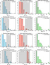 |
Fig. A.1. Distribution of physical properties across the TNG300 sample. The histograms show the frequency of gas mass (left), stellar mass (center), and SFR (right). The vertical shaded bands represent the observational uncertainties for the targeted clusters. The vertical dashed lines indicate the specific values of the best matches identified by the Siamese CNN. |
To evaluate the physical consistency of the Siamese CNN’s selections, we calculated the number of simulated halos that simultaneously satisfy the observed constraints for all three physical parameters (Mgas, M★, and SFR). For the Virgo cluster, out of the 40 parent halos, 15 satisfy the combined physical bounds, with the CNN-selected best match falling within this subset. Similarly, we find that five halos meet all three physical criteria for the Centaurus cluster, while six and 12 halos satisfy the combined constraints for Ophiuchus and A3266, respectively. The high degree of overlap between the kinematically selected best matches and these physically allowed regions demonstrates that the Siamese network identifies candidates that are not only morphologically similar but also physically representative of the observed systems. The high degree of overlap between the kinematically selected best matches and the physically allowed parameter space demonstrates that the Siamese CNN effectively captures the underlying physics of the ICM without explicit prior informing on global mass or star-formation scales. This confirms that the learned embeddings are physically meaningful and not merely capturing coincidental morphological similarities.
All Tables
Summary of TNG300 halo properties from the best matches between XMM-Newton observations and simulated clusters.
All Figures
|
Fig. 1. Diagram of the CNN architecture used in our analysis. The network processes 128 × 128 × 1 input velocity maps through a series of convolution and max-pooling layers to extract hierarchical features. The resulting feature map is flattened and passed through a fully connected dense layer of 512 units, culminating in a 128D embedding vector that provides a compact, discriminative representation of the cluster kinematics. |
| In the text | |
|
Fig. 2. Diagram of the Siamese CNN training phase. During training, triplets of velocity maps are passed through identical CNN encoders with shared weights. Each triplet consists of a reference (Anchor), a matched projection from the same simulated cluster (Positive), and a mismatched projection from a different simulated cluster (Negative). The network learns to produce similar embeddings for the Anchor–Positive pairs and dissimilar embeddings for the Anchor–Negative pairs by minimizing the triplet loss. This process teaches the model to recognize the underlying kinematic structure of clusters, independent of projection and resolution differences. |
| In the text | |
|
Fig. 3. Diagram of the Siamese CNN matching phase. During matching, the trained Siamese CNN compares each observed XMM-Newton velocity map to the full library of simulated velocity maps. Both the observed map and each simulated cluster are passed through the shared-weight CNN encoder to generate corresponding embedding vectors. Similarity between the observation and a given simulated cluster is quantified by the distance between their embeddings in the learned latent space. Simulated clusters with the smallest embedding distance are identified as the closest kinematic matches, enabling a quantitative, model-driven comparison between observed cluster dynamics and the cosmological simulations. |
| In the text | |
|
Fig. 4. t-SNE plots comparing the observed velocity maps of four galaxy clusters to the TNG simulation library. While all embeddings were generated using a single trained Siamese CNN, we present independent t-SNE projections for each source to clearly visualize the specific matches within the broader simulated distribution. Points represent the relative similarity of velocity maps in the latent space, with proximity indicating a closer kinematic match. The nonuniform distribution of the TNG-simulated clusters reflects underlying physical gradients and evolutionary sequences learned by the network. The axes are arbitrary, and quantitative similarity rankings (blue) are calculated based on Euclidean distances in the original high-dimensional embedding space rather than these 2D stochastic projections. |
| In the text | |
|
Fig. 5. Best-matching velocity maps from the TNG300 simulated clusters obtained with the Siamese CNN analysis for the XMM-Newton observations. The zoom-in panel shows the XMM-Newton data for a region centered on the physical origin (0, 0 kpc) of the simulated cluster. All simulated maps are presented at a fixed physical scale to maintain consistency across the sample. The apparent difference in coverage between the panels (e.g., A3266 vs. Virgo) is a result of the different angular sizes and distances of the observed clusters. Showing the full simulated extent provides crucial context for the large-scale dynamics and merger history that drive the observed core kinematics, offering insights into the broader physical environment of the matched systems. These figures illustrate kinematic similarity based on the CNN-learned metric, rather than pixel-wise visual resemblance. |
| In the text | |
|
Fig. A.1. Distribution of physical properties across the TNG300 sample. The histograms show the frequency of gas mass (left), stellar mass (center), and SFR (right). The vertical shaded bands represent the observational uncertainties for the targeted clusters. The vertical dashed lines indicate the specific values of the best matches identified by the Siamese CNN. |
| In the text | |
Current usage metrics show cumulative count of Article Views (full-text article views including HTML views, PDF and ePub downloads, according to the available data) and Abstracts Views on Vision4Press platform.
Data correspond to usage on the plateform after 2015. The current usage metrics is available 48-96 hours after online publication and is updated daily on week days.
Initial download of the metrics may take a while.