| Issue |
A&A
Volume 710, June 2026
|
|
|---|---|---|
| Article Number | A105 | |
| Number of page(s) | 11 | |
| Section | The Sun and the Heliosphere | |
| DOI | https://doi.org/10.1051/0004-6361/202558675 | |
| Published online | 03 June 2026 | |
3D reconstruction of thermal hard X-ray sources in solar flares from combined STIX and HXI visibilities
1
MIDA, Dipartimento di Matematica, Università di Genova, via Dodecaneso 35, I-16146, Genova, Italy
2
University of Applied Sciences and Arts Northwestern Switzerland (FHNW), School of Computer Science, Bahnhofstrasse 6, Windisch, 5210, Switzerland
3
Swiss Federal Institute of Technology in Zurich (ETHZ), Rämistrasse 1, 8001, Zürich, Switzerland
4
University College London, Mullard Space Science Labratory, Holmbury St Mary, Dorking, Surrey, RH5 6NT, UK
5
Division of Dark Matter and Space Astronomy, Purple Mountain Observatory, Chinese Academy of Sciences (CAS), Nanjing, 210023, China
6
School of Astronomy and Space Science, University of Science and Technology of China, Hefei, 230026, China
7
Istituto Nazionale di Astrofisica, Osservatorio Astrofisico di Torino, via Osservatorio 20, 10025, Pino Torinese, Italy
8
Space Sciences Laboratory, University of California, 7 Gauss Way, 94720, Berkeley, USA
★ Corresponding authors: This email address is being protected from spambots. You need JavaScript enabled to view it.
; This email address is being protected from spambots. You need JavaScript enabled to view it.
; This email address is being protected from spambots. You need JavaScript enabled to view it.
Received:
19
December
2025
Accepted:
29
April
2026
Abstract
Context. The Spectrometer/Telescope for Imaging X-rays (STIX) on board the ESA Solar Orbiter mission and the Hard X-ray Imager (HXI) aboard the Advanced Space-based Solar Observatory (ASO-S) satellite provide for the first time systematic coverage of solar flare hard X-ray sources from different vantage points. This unprecedented configuration enables the reconstruction of the three-dimensional (3D) hard X-ray intensity distribution of the thermal emission in solar flares.
Aims. The main objectives of this study are twofold: (1) to perform 3D reconstructions of the thermal hard X-ray source of a solar flare using stereoscopic Fourier data (visibilities) provided by STIX and HXI; and (2) to investigate the evolution in time of the reconstructed 3D source morphology.
Methods. The sets of 2D visibilities measured by STIX and HXI represent a sampling of the 3D Fourier transform of the flaring hard X-ray source on two planes orthogonal to the instruments’ lines of sight. Therefore, the 3D reconstruction problem is analogous to the standard 2D imaging problem and can be addressed with similar techniques. In this case, we performed 3D reconstructions by means of the iterative space reconstruction algorithm (ISRA).
Results. We consider the SOL2024-10-03T12:12 event observed by STIX and HXI from largely different vantage points separated by 85.7°. We performed 3D reconstructions of the flaring thermal emission at a 10 s cadence, and we determined the X-ray source height and radial velocity over time. As a consistency test, we show that the morphology and location of our 3D reconstructions are consistent with the corresponding 2D images independently obtained from STIX and HXI data.
Conclusions. The proposed 3D reconstruction methodology provides reliable results for events with a separation angle close to 90°. However, the dynamic range of the 3D reconstructions is limited by the low number of observed visibilities (as in the 2D case) and by the limited number of vantage points on the flaring events.
Key words: methods: numerical / techniques: image processing / Sun: flares / Sun: X-rays / gamma rays
© The Authors 2026
 Open Access article, published by EDP Sciences, under the terms of the Creative Commons Attribution License (https://creativecommons.org/licenses/by/4.0), which permits unrestricted use, distribution, and reproduction in any medium, provided the original work is properly cited.
This article is published in open access under the Subscribe to Open model. This email address is being protected from spambots. You need JavaScript enabled to view it. to support open access publication.
1. Introduction
Understanding the three-dimensional (3D) structure and evolution of solar flares is critical for interpreting the physical processes that drive their dynamics. In the classical standard flare model (Carmichael 1964; Sturrock 1966; Kopp & Pneuman 1976), magnetic energy release accelerates particles in the corona, producing both nonthermal and thermal X-ray emission. Nonthermal electrons propagate along magnetic field lines and deposit energy in the chromosphere, giving rise to hard X-ray (HXR) footpoints. The heated plasma rises from the chromosphere and fills the flare loops, where it produces thermal X-ray emission. Therefore, knowledge of the 3D intensity distribution of the thermal X-ray sources allows us to localize the hottest plasma within the coronal magnetic structures and to study its spatial and temporal evolution. The height and volume of these sources, and their variation during the flare, provide key constraints on the geometry of magnetic reconnection and on the energetics of the flaring plasma.
To date, most solar flare HXR imaging has been performed with indirect Fourier imaging systems. A small number of directly focused observations have been achieved (e.g., Krucker et al. 2014; Glesener et al. 2017) using grazing incidence optics (Wolter 1952). Obtaining a greater number and quality of such observations is a key goal for the future of high-energy solar physics, due to the unique observational capabilities they provide. However, indirect Fourier imaging systems enable more compact instrument designs and imaging to much higher energies (e.g., Prince et al. 1988; Hurford 2013). They have therefore formed the basis of previous and current satellite-based solar HXR imagers.
The measurements provided by these instruments can be mathematically described as two-dimensional (2D) Fourier components of the LOS-integrated X-ray intensity distribution (e.g., Zhang et al. 2019; Massa et al. 2023), where LOS denotes line of sight. Analogous to the context of radio interferometry (e.g., Thompson et al. 1992), these components are called “visibilities”. Therefore, the data provided by a single telescope allow for the reconstruction of the 2D LOS-integrated intensity distribution of the flaring X-ray sources by solving an inverse imaging problem (e.g., Piana et al. 2022). Until recently, reconstructions of the 3D intensity distribution of solar flare X-ray sources1 were not feasible due to the lack of simultaneous observations from multiple vantage points. As a result, the morphology of flare X-ray sources has always been reconstructed in two dimensions, relying on observations from a single instrument. In this framework, crucial flare properties such as source height and radial motion could be roughly estimated only for limb events (e.g., Gallagher et al. 2002).
Several studies have investigated the 3D reconstruction of coronal structures using stereoscopic observations in the ultraviolet (UV) and extreme ultraviolet (EUV) bands, particularly from the Solar Terrestrial Relations Observatory (STEREO) mission (e.g., Aschwanden et al. 2008b,a, 2009, 2012). These methods have provided valuable insights into the morphology and topology of coronal loops in active regions, as well as into the density and temperature structure of the ambient coronal plasma. More recently, data-driven and machine-learning-based approaches such as neural radiance fields (NeRFs) have been proposed to perform volumetric 3D reconstructions of the EUV corona (Jarolim et al. 2024). However, these techniques are intrinsically limited to relatively cool plasma (∼1–2 MK), and therefore lack sensitivity to the hottest, X-ray-emitting components. In addition to EUV coronal reconstructions, several works have focused on the 3D reconstruction of coronal mass ejections (CMEs) using stereoscopic coronagraphic and heliospheric imaging. Notably, Byrne et al. (2010) introduced an elliptical tie-pointing technique that allows the full 3D geometry of CME fronts to be recovered from STEREO observations.
The possibility of performing 3D reconstructions of HXR sources has emerged thanks to the launch of the ESA Solar Orbiter mission (Müller et al. 2020), which observes the Sun from a vantage point significantly offset from Earth for most of the time. The first 3D reconstruction of a thermal X-ray source morphology was presented by Ryan et al. (2024a). They combined HXR images reconstructed from data provided by the Spectrometer/Telescope for Imaging X-rays (STIX; Krucker et al. 2020) on board Solar Orbiter with soft X-ray images from Hinode’s X-Ray Telescope (XRT; Golub et al. 2008; Kosugi et al. 2008). In this study, the authors modeled the emitting structure as a stack of elliptical cross-sections arranged by using the elliptic tie-pointing method. The shape and extent of each ellipse in the stack were determined by matching the outer contours of the images of X-ray sources that are provided by the two instruments. One drawback of this approach is that XRT is not a spectroscopic imager: it observes in broad, filter-based passbands that are sensitive to plasma at different temperatures, but do not allow narrow energy selection. STIX, on the other hand, is a spectroscopic imager capable of energy-resolved imaging. As a result, combining STIX and XRT data for 3D reconstructions is only possible under the assumption that both instruments observe the same plasma population, and verifying this condition is not always straightforward due to the multi-thermal nature of solar flares (e.g., Warren et al. 2013). Further, from a methodological viewpoint, in this case the reconstructions are based on STIX images, which are themselves obtained through inversion algorithms, so that the resulting geometry can be influenced by the choice of reconstruction method. In addition, this method requires the emitting structure to be represented as a stack of ellipses, which inevitably constrains the possible volume shapes.
The first analysis of stereoscopic observations provided by two HXR telescopes was presented by Ryan et al. (2024b). They considered data of the same X-class flare collected by STIX and by the Hard X-ray Imager (HXI; Zhang et al. 2019; Su et al. 2019, 2024), which operates in a low Earth orbit on board the Advanced Space-based Solar Observatory mission (ASO-S; Gan et al. 2019, 2023). The 3D location of thermal and nonthermal X-ray sources was determined by triangulating the centroid positions of the 2D reconstructions independently obtained from STIX and HXI data. However, in this case, 3D reconstructions were not feasible as the separation angle between the two observatories and the flaring site was only ∼20°.
In this work, we present the first 3D reconstructions of solar flare thermal HXR sources from a combined set of visibilities provided by STIX and HXI. We focus on the SOL2024-10-03T12:12 flare event as the separation angle between STIX, the flaring site, and HXI is close to 90°, which is the ideal configuration for 3D reconstructions (Ryan et al. 2024a). We show that 2D visibilities measured by STIX and HXI can be interpreted as 3D Fourier components of the flaring X-ray sources sampled on planes orthogonal to the instruments’ LOS in the 3D spatial frequency space. We applied the iterative space reconstruction algorithm (ISRA; Daube-Witherspoon & Muehllehner 1986) to the joint set of visibilities to obtain the 3D reconstruction of the thermal flaring source. From this reconstruction, we derived estimates of the source height and radial motion, and analyzed the temporal evolution of its morphology.
Our methodology differs in several respects from the approach presented by Ryan et al. (2024a). In fact, here we work directly with the visibilities measured by STIX and HXI, avoiding the intermediate use of 2D image reconstruction methods. In addition, our technique does not impose any predefined source morphology. At the same time, both approaches provide most reliable results in the case when the separation angle between the two instruments is close to 90°. In fact, although it is always possible to obtain a 3D reconstruction when the two instruments have a different vantage point, the reconstruction uncertainty becomes extremely large once the angle between the two telescopes and the flaring site is either less than 70° or more than 110° (see discussion in Ryan et al. 2024a). Therefore, the number of solar flare events that can be analyzed with stereoscopic techniques is very limited.
The structure of this paper is as follows. In Sect. 2 we provide an overview of the SOL2024-10-03T12:12 event and we describe the data considered for this study. In Sect. 3 we describe the methodology we implemented to perform 3D reconstructions of thermal X-ray sources. Section 4 contains the 3D reconstruction results and a comparison with the 2D images independently obtained from STIX and HXI data. In Sect. 5 we discuss limitations of our indirect imaging techniques and caveats in the interpretation of the reconstruction volumes for the study of flare energetics. Finally, Sect. 6 contains our conclusions.
2. STIX and HXI data
In this section, we present an overview of the solar flare SOL2024-10-03T12:12, where the time indicates the start time of the event as recorded at Earth by the Geostationary Operational Environmental Satellite (GOES). Further, we describe the methodology we adopted to correct for inaccuracies in the pointing information provided by STIX and HXI. Finally, we verify that the counts recorded by both instruments in the energy range we considered for 3D reconstructions (14–18 keV) are mainly produced by the same thermal source and can therefore be used for the 3D reconstruction task.
2.1. Event overview
The X9.1 GOES class flare originated in active region NOAA 13842, and was observed simultaneously by HXI, in a low Earth orbit, and by STIX, on board Solar Orbiter. At the time of the flare, Solar Orbiter was located at Stonyhurst heliographic coordinates of longitude −84.8° and latitude −0.1°, and at a heliocentric distance of 0.29 AU. Additionally, STIX was positioned −3.8° below the Earth’s ecliptic plane, offering a slightly out-of-ecliptic vantage point. This geometry resulted in a separation angle of approximately 85.7° between STIX and HXI with respect to the flaring region (see Fig. 1A). From STIX and HXI the flare is seen with an angle of 89° and 22° with respect to the solar surface normal, respectively. Since the two instruments were located at different distances from the Sun, they observed the same event at different times. Therefore, the STIX times have been adjusted by adding the difference in light travel time between the Sun–Earth and Sun–STIX and paths (350 s) to ensure proper temporal alignment with HXI and GOES observations. In the remainder of the paper, the reported times refer to Earth-based time.
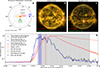 |
Fig. 1. Overview of the SOL2024-10-03T12:12 event. (A) Schematic illustration (not to scale) showing the relative positions of STIX, HXI, and the flaring region. (B) EUI 174 Å image from Solar Orbiter, with the apparent solar limb as viewed from HXI overlaid in green for reference. (C) Full-disk AIA 171 Å image, with the apparent solar limb from the STIX viewpoint overlaid in green. In panels (B) and (C) the flaring active region is highlighted with a light red square. The EUI and AIA images are observed at 12:16:45 and 12:16:33 UT, respectively. (D) Normalized light curves: GOES 1–8 Å channel (red), STIX 14–18 keV (yellow) as measured by the Background detector (BKG; Krucker et al. 2020), STIX 36–76 keV (blue) as measured by the imaging detectors, HXI 14–18 keV (magenta), and HXI 36–76 keV (black). The shaded gray area indicates the time interval considered in the analysis, while the shaded blue and red areas indicate the time ranges considered for the reconstructions of Figures 2 and 3, respectively. Times are expressed as light arrival times at Earth. |
Figures 1B and 1C show full-disk EUV images of the Sun from the vantage points of STIX and HXI, respectively. Panel B displays a 174 Å image recorded by the Full Sun Imager of the Extreme Ultraviolet Imager (EUI/FSI; Rochus et al. 2020) on Solar Orbiter, while panel C shows a 171 Å image from the Atmospheric Imaging Assembly (AIA; Lemen et al. 2012) on board the Solar Dynamics Observatory (SDO; Pesnell et al. 2012). The flare location is highlighted by a red square in both panels. From the STIX viewpoint the active region appears located directly at the solar limb, whereas from the HXI vantage point it is observed close to disk center, slightly below the equator. We display in Figure 1D the light curves provided by STIX, HXI, and GOES, which show the temporal evolution of the event. The shaded gray region marks the time interval selected for 3D reconstructions we performed at a 10 s cadence. This time range, which spans from 12:14:55 to 12:26:15 UT, covers the late impulsive phase, the flare peak, and the early decay phase.
2.2. Co-alignment with HMI data
Figures 2A and 2B show X-ray images corresponding to the time interval between 12:15:10 and 12:15:50 UT as reconstructed from STIX and HXI data, respectively. Red contours indicate the thermal emission in the 14–18 keV energy band, while blue contours correspond to the nonthermal emission in the 50–100 keV range. The images of the nonthermal emission were reconstructed by means of the CLEAN algorithm (Högbom 1974; Su et al. 2019). For STIX, we considered the sub-collimators with an angular resolution larger than 14″ (see, e.g., Massa et al. 2022), while for HXI we considered collimators with an angular resolution larger than 6″. The thermal emission appears spatially extended, and the CLEAN algorithm could artificially break it into separate sources if the CLEAN beam width were not appropriately selected. To avoid problems with the selections of the beam width, we decided to apply the MEM_GE algorithm (Massa et al. 2020) to perform reconstructions in the 14–18 keV energy range for both STIX and HXI. Further, as the fine-resolution detectors show limited modulation, we considered only those with a resolution larger than 40″ and 13″ for STIX and HXI, respectively. Given the different distances between STIX and HXI from the Sun, the sets of visibilities selected for the two instruments correspond to comparable spatial resolution.
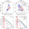 |
Fig. 2. Imaging and spectral analysis of the SOL2024-10-03T12:12 event. Panels (A) and (B): Reconstructions obtained from STIX and HXI data between 12:15:10 and 12:15:50 UT. The contours of the reconstructions in the 14–18 keV and in the 50–100 keV energy ranges are plotted in red and blue, respectively. In both panels, contours are plotted at 30%, 50%, 70%, and 90% of the peak intensity in each energy band. The reconstructions are overlaid to a difference image of the continuum acquired by HMI at 12:14:45 and 12:15:30 UT. For reference, the same semicircular loop model (cyan) is plotted in both panels as seen from the corresponding vantage points. Panels (C) and (D): Spectra recorded by STIX and HXI, respectively, in the time range between 12:15:30 and 12:15:40 UT. A thermal (red), nonthermal (blue), and albedo (gray) component was fit to each observed spectra (in black) in the energy range 12–100 keV. The total fit is shown in green, and the reduced χ2 value of the fit is printed in the top part of each panel. The energy range used for 3D reconstructions is highlighted in red. All times above are expressed as light arrival times at Earth. |
The currently available STIX pointing measurement for this flare is only accurate to tens of arcseconds. Therefore, to determine appropriate corrections to the STIX pointing and accurately locate the reconstructions on the plane of the sky, we aligned the STIX images with imaging data provided by the Helioseismic and Magnetic Imager (HMI; Scherrer et al. 2012) on board the SDO. We considered continuum images recorded by HMI at 12:14:45 UT and 12:15:30 UT. The difference of these images, plotted in the background of Fig. 2B, shows the flare ribbons in white light, which are known to be almost co-spatial with HXR footpoints (e.g., Kuhar et al. 2016). We identified the expected HXR footpoint locations and we connected them with a semicircle2 representing the simplest possible magnetic field configuration (plotted in cyan in Fig. 2B). We reprojected the HMI difference image to the vantage point of Solar Orbiter using the astropy reproject3. The reprojected difference image is displayed in Fig. 2A. The white light ribbons appear foreshortened from the STIX vantage point, since they are close to the limb (see Fig. 2B). We manually shifted the location of STIX HXR footpoints to be close to the base of the reprojected semicircle and slightly offset with respect to the photospheric limb to take into account that such X-ray emission occurs in the lower chromosphere (e.g., Krucker et al. 2015). Overall, the center of the STIX image was shifted by (45″, 85″).
Although the HXI pointing accuracy is usually better than 1″ (Zhang et al. 2019; Su et al. 2019), the contour levels of the HXI footpoints were slightly offset with respect to the white light ribbons visible in the HMI images. We attribute these errors to incomplete calibration in both aspect information and visibility data. Therefore, we manually shifted the HXI reconstructions by (2″, 2″), a value much smaller than the finest resolution of the sub-collimators adopted for the reconstruction of the image (13.4″).
Inaccuracies on the position of the reconstructed STIX and HXI images on the solar disk are due to a bias between imaging and pointing information, the latter provided by the instruments’ aspect system. While this bias does vary over time (at least, at the current stage of calibration of the aspect data), variations occur over timescales of hours or days. Therefore, the same pointing correction can be applied to every 10 s time interval considered for the 3D reconstructions. This is standard practice. After co-alignment with HMI maps, uncertainty on the image location is very limited (1–2″ see Ryan et al. 2024b).
2.3. Energy range selection and visibility normalization
For the 3D reconstructions of the thermal emission (see Sect. 4 below), we considered data integrated in the energy range 14–18 keV for both instruments. During the considered time intervals, STIX was operating with its attenuator in place. In this configuration, the thermal response functions of STIX and HXI are expected to be broadly comparable; for details, see Ryan et al. (2024b).
To investigate whether the emission registered by both instruments in this energy range originates from the same volume of hot plasma, we performed spectral analysis on the spectra recorded by STIX and HXI individually. We selected the time interval between 12:15:30 and 12:15:40 UT (which is around the main nonthermal peak) and we fit an isothermal model, a nonthermal thick target model, and an albedo component. The results are shown in Figs. 2C and D. The spectral analysis confirms that the 14–18 keV count flux (highlighted in red) is dominated by thermal emission. However, more details on the contribution of the nonthermal and albedo components in this energy range are provided in Sect. 5.1. Note that we performed this spectral analysis to qualitatively show that the X-rays detected in the 14–18 keV energy range are mainly produced by thermal emission. A quantitative comparison between the STIX and HXI spectral fitting analyses can be found in Li et al. (2025).
As the observed visibilities are in count units (and not in photon units), we normalized the STIX and HXI visibility sets with respect to their own maximum amplitudes. This normalization removed the dependencies on the instrument responses. The resulting reconstructions therefore do not contain information on the total photon flux.
3. Methodology
Both STIX and HXI are indirect imaging instruments designed to detect HXR emission from solar flares by counting individual photons that reach the detector after being emitted by the source. Since each instrument collects all photons arriving from a given direction, regardless of where along the LOS they were emitted, the measured signal is inherently sensitive to the angular distribution of the source on the plane of the sky. Both STIX and HXI use a double-grid system to spatially encode the incoming flux, which is then measured by photon-counting detectors, although STIX and HXI differ in their modulation strategies. STIX uses pairs of tungsten grids placed in front of each detector, with a small difference in orientation angle and pitch between the front and the rear grid. As photons pass through this offset configuration, Moiré patterns are formed on the detector surface. These patterns encode spatial information about the source in terms of spatial frequency and orientation (Massa et al. 2023). HXI also employs a bi-grid system, but implements a different modulation strategy. Specifically, a pair of sub-collimators having a front and rear grid with identical orientation angle and pitch, but different relative positions, are used to measure the real and the imaginary part of the same visibility (Su et al. 2019). For both instruments, and under the small-angle approximation (which is valid given the large Sun–spacecraft distance relative to the flare size), the photon count modulation can be mathematically processed to extract the complex value of the visibilities, i.e., the 2D Fourier components of the LOS-integrated X-ray emissivity.
Let ϕ(x), with x ∈ ℝ3, denote the 3D photon emissivity, i.e., the number of photons emitted per unit volume at position x. We denote by ϕθ the 2D LOS-integrated emissivity, where θ ∈ ℝ3 indicates the LOS direction in the 3D space. The measured visibilities are then defined as
, \end{aligned} $$](/articles/aa/full_html/2026/06/aa58675-25/aa58675-25-eq1.gif) (1)
(1)
where ℱ2D denotes the 2D Fourier transform, and (u, v)∈θ⊥ are the frequencies determined by the instrument’s collimator geometry. Here, θ⊥ indicates the plane perpendicular to the LOS direction, θ. Each instrument therefore samples a 2D slice of the 3D Fourier frequency space, orthogonal to its LOS. By combining data from two instruments observing the same flare from different vantage points, it is possible to obtain visibility measurements on two distinct planes in the 3D Fourier domain. Therefore, the 3D reconstruction problem consists of determining the function, ϕ(x), such that
 , \quad \text{ for} (u, v) \in \theta _i^\perp , \quad i = 1, 2, \end{aligned} $$](/articles/aa/full_html/2026/06/aa58675-25/aa58675-25-eq2.gif) (2)
(2)
where θ1 and θ2 represent the LOS directions of STIX and HXI, respectively. Since the visibilities are complex numbers, we reformulated the problem as a real-valued system by separating the real and imaginary parts and stacking them vertically. In this representation, the discretized imaging problem becomes
 (3)
(3)
where  is the unknown emissivity vector (n being the total number of voxels),
  is the array of visibilities measured by STIX and HXI (m being the total number of real and imaginary parts of the visibilities), and
  represents the discretization of the Fourier transform, ℱ3D, computed in the frequencies sampled by STIX and HXI.
Reconstructing the 3D X-ray emission by solving Eq. (3) is an ill-posed inverse problem (Bertero et al. 2021), which we address by means of the ISRA (Daube-Witherspoon & Muehllehner 1986). The ISRA method is a classical algorithm for solving linear inverse problems with non-negative solutions (such as the emissivity vector Φ) and has been successfully applied in both astronomical and medical imaging contexts (e.g., Anconelli et al. 2006; Titterington 1987). The ISRA update rule (e.g., Zunino et al. 2009) is given by
 (4)
(4)
where the numerator and denominator are defined as
 (5)
(5)
 (6)
(6)
Here, (·)+ and (·)− denote the positive and negative parts of a vector, respectively, while the terms F± represent the positive and negative parts of the matrix F, defined component-wise. Reconstructions were performed for 100 iterations in all cases presented.
4. Results
We performed 3D reconstructions of the SOL2024-10-03T12:12 thermal X-ray source using visibilities in the 14–18 keV energy range. For both STIX and HXI, we considered the same sets of sub-collimators as those selected for the reconstruction of the thermal emission discussed in Section 2.2. This choice results into 15 visibilities for STIX and 26 visibilities for HXI. The analysis covered the time interval from 12:14:55 to 12:26:15 UT, with 10 s integration windows The choice of 10 s integration time ranges reflects a compromise between achieving a high time cadence and ensuring sufficient counting statistics.
4.1. 3D visualization of the thermal X-ray source
As an example, Figure 3 shows the 3D reconstruction obtained from combined STIX and HXI visibilities integrated between 12:16:35 UT and 12:16:45 UT. The same reconstructed HXR source is rendered as viewed from five different vantage points: Solar Orbiter, the Lagrangian point L5, ASO-S, Solar–TErrestrial RElations Observatory (STEREO-A; Kaiser et al. 2008), and Mars. For contextual reference, each rendering is overlaid to an HMI difference image highlighting the photospheric flare ribbons. The yellow-to-red shaded surfaces in the figure represent isosurfaces of the reconstructed emission at 30%, 50%, 70%, and 90% of the peak intensity. These isosurfaces were obtained from the 3D voxel grid using the marching_cubes4 function from the scikit-image library (van der Walt et al. 2014), and rendered through the sunpy sunkit-pyvista5 visualization framework (The SunPy Community et al. 2020). Semitransparency was applied to allow the internal structure of the reconstructed volume to remain visible. To provide a 3D visual impression of the reconstruction, shadows obtained by illuminating the 3D scene from the viewpoint of the observer were included.
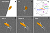 |
Fig. 3. 3D reconstruction of the thermal X-ray emission of the SOL2024-10-03T12:12 event in the time range between 12:16:35 and 12:16:45 UT, and in the energy range 14–18 keV. Panels (A), (B), (D), (E), and (F) show the reconstructed X-ray source as viewed from Solar Orbiter, L5, ASO-S, Stereo-A, and Mars, respectively. The yellow-to-red surfaces represent isosurfaces at 30%, 50%, 70%, and 90% of the peak intensity. To render the 3D morphology of the reconstructed X-ray emission, shadows are included by illuminating the 3D source from the observer’s viewpoint. In each panel, we also display the difference between the HMI continuum images at 12:16:15 and 12:15:30 UT, which show the flare ribbons in white light. Finally, Panel (C) shows the relative positions of the considered spacecrafts, planets, and Lagrangian points with respect to the Sun. The associated movie is available online. |
An animation is provided in the supplementary material to illustrate the temporal evolution of the 3D reconstruction. Each frame was constructed in the same way as for Fig. 3, where the 3D volumes are represented through intensity isosurfaces at each time step. The difference continuum image from HMI is also included but with a lower time cadence (45 s) compared to HXR reconstructions (10 s). Therefore, several consecutive 3D reconstructions share the same HMI difference image.
In the whole animation, the lowest-intensity isosurfaces (at 30% of the peak intensity) present artefacts that probably due to the limited amount of data available for image reconstruction (both in terms of number of visibilities and number of vantage points) and to propagation of noise during the reconstruction process. Initially, the reconstructed volume appears elongated, before becoming more compact after ∼12:15:35 UT. At ∼12:16:55 UT, the source elongates again, coincident with the displacement of the flare ribbons visible in the HMI data, and subsequently returns to a compact configuration around ∼12:18:55 UT. During the late phase of the flare peak, the reconstructed volume expands once more. In addition, the animation clearly shows a progressive increase in the altitude of the reconstructed source throughout the flare evolution (a more detailed discussion is provided in Sect. 4.3).
4.2. Consistency check with 2D reconstructions
In order to compare the 3D reconstructions with the 2D reconstructions independently obtained from STIX and HXI, we integrated the 3D emission along the LOS of both instruments. Figure 4 illustrates this comparison in the case of the reconstructions obtained from data recorded between 12:16:35 and 12:16:45 UT. Figures 4A–C correspond to the HXI viewpoint: Figure 4A displays the 3D reconstruction rendered from the HXI perspective; Figure 4B shows the contour levels of the 3D reconstruction integrated along the HXI LOS; and Figure 4C directly compares the contours of the integrated 3D reconstruction (in red) with those derived from the 2D MEM_GE reconstruction (in blue). Panels D–F present the same sequence of visualizations for the STIX perspective.
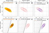 |
Fig. 4. Comparison between 3D and 2D reconstructions of the thermal flare emission in the 14–18 keV energy band at 12 : 16 : 35 UT. Panels A–C show the HXI viewpoint: (A) 3D reconstruction viewed from the HXI perspective; (B) contour levels of the 3D reconstruction integrated along the HXI LOS; (C) contours of the 3D reconstruction integrated along the HXI LOS (red) and of the 2D reconstruction obtained from HXI data only (blue). Panels D–F are the same as A–C but for the STIX viewpoint: (D) 3D reconstruction; (E) contour levels of the 3D reconstruction integrated along the STIX LOS; (F) contours of the 3D reconstruction integrated along the STIX LOS (red) and of the 2D reconstruction obtained from STIX data only (blue). All contour levels and isosurfaces correspond to 30%, 50%, 70%, and 90% of the respective peak intensity. The associated movie is available online. |
A supplementary animation provides a side-by-side comparison of the 3D reconstructions with the corresponding 2D reconstructions independently obtained from STIX and HXI data, extending the analysis of Fig. 4 to the entire sequence of time intervals considered. This enables a direct visual assessment of the consistency between the multi-vantage-point and single-instrument imaging approaches over time. A qualitative comparison of the 3D isosurfaces at 30% of the peak intensity with the corresponding 2D contours shows that the 3D structure generally encloses a larger area than the HXI contours, but a smaller one than those from STIX. This discrepancy may be partly explained by the reduced reliability of the lowest-intensity contours. At levels of 50% and higher, the agreement with the 2D reconstructions improves significantly. Overall, the source position inferred from the 3D reconstructions remains spatially consistent with the reconstructions from both STIX and HXI.
Table 1 summarizes a quantitative comparison between the 3D reconstructions integrated along the LOS of the telescopes and the corresponding 2D reconstructions in terms of source centroids and areas. For the centroid analysis, we computed the centroid of the region enclosed by the 50% contour6 at each time step, defined as
 (7)
(7)
Centroid offset and IoU metric comparing the 2D reconstructions independently obtained from STIX and HXI data with the 3D reconstructions integrated along their respective instrument LOS.
where Ω denotes the area within the 50% contour, and ϕθ(x) is the photon intensity in the 2D image. In the case of 3D reconstructions, this corresponds to the LOS-integrated emissivity, while for 2D reconstructions it is the directly reconstructed intensity. The values reported in Table 1 (first row) correspond to the mean and standard deviation over the different time ranges of the centroid offset between the LOS-integrated 3D reconstructions and the 2D images independently reconstructed from STIX and HXI data.
We evaluated the similarity between the regions enclosed within the 50% contour of the 2D single-instrument reconstructions (R2D) and of the corresponding LOS-integrated 3D reconstructions (R3D los) by using the intersection over union metric (IoU; Rezatofighi et al. 2019):
 (8)
(8)
where | ⋅ | denotes the area of the region. The IoU metric equals 1 when the two regions perfectly coincide, and approaches 0 when they are largely dissimilar. The reported values in the second row of Table 1 are the mean and standard deviation of the metric over the different 10 s time ranges considered in the analysis.
The results reported in Table 1 show that the centroid positions of the LOS integrated 3D reconstructions are in agreement with those of the 2D images independently reconstructed from STIX and HXI. Indeed, the discrepancy between these locations is on average up to ∼10% of the finest resolution considered for image reconstruction for both instruments (40″ for STIX and 13.4″ for HXI; see Sect. 2.2). Further, the regions enclosed within the 50% contours of the LOS integrated 3D reconstructions, and the regions enclosed within the 50% contours of 2D images independently reconstructed from STIX and HXI data, have an overlapping area that is only ∼70% of the combined area. This is not surprising given the limited dynamic range of these indirect imaging techniques and given that different algorithms were used for 3D and 2D reconstructions (ISRA and MEM_GE, respectively), which can lead to slightly different results. Therefore, the IoU metric shows that 3D and 2D reconstructions are in fact consistent within the limitations of these challenging imaging problems.
4.3. Height and radial velocity analysis
To analyze the evolution of the height and radial motion of the thermal X-ray source during the flare, we first quantified the source position at each time step by computing the centroid,  , of the emission enclosed within the 50% intensity isosurface of the 3D reconstruction, using Eq. (7) but applied to volumes rather than areas. The radial distance of the centroid from the center of the Sun was then calculated, and the source height was defined as the difference between this value and the standard photospheric radius. Figure 5 shows the temporal evolution of the reconstructed source height. The height increases steadily throughout the event as expected in a reconnection-driven scenario where flare loops at higher and higher altitudes are created in time. The decrease seen around 12:17:25 UT is associated with the emergence of a new thermal source to the southwest (see movie in the supplementary material). We associate the new source with a strengthening of the reconnection process in the southwest part of the flare ribbon, which appears to be at a slightly lower altitude. The computed centroid position corresponds to the intensity-weighted mean of old and new source. As a result, the centroid shows an apparent motion towards lower altitudes, followed by an increasing motion reflecting the increasing altitude of the reconnection process at the new source location. Overall, the height of the thermal X-ray source ranges from approximately 6 Mm to 14 Mm over the analyzed time interval. These results are comparable to those by Ryan et al. (2024a), who found heights of between 8 and 15 Mm.
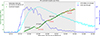 |
Fig. 5. Temporal evolution of the 3D centroid height above the solar surface for the flare SOL2024-10-03T12:12. The individual height values are plotted as green circles, while the average radial velocities for several identified time ranges are indicated both in black and in red. Each velocity value corresponds to the average speed between the first and the last time step of each black or red line, which indicates a time range with approximately constant velocity. As a reference, the STIX light curves for the 14–18 keV and for the 36–76 keV energy ranges are plotted in cyan and in blue, respectively. The left and right vertical axes refer to the centroid height and the normalized STIX flux, respectively. |
To estimate the radial velocity of the source, we avoided computing differences between consecutive time steps, which are strongly affected by short-term fluctuations in height. Instead, we calculated the average velocity over broader time intervals, selected to capture the overall upward trend. These trends are represented as black and red lines in Figure 5. In particular, we found that the radial velocity exhibits significant variability over the course of the event, with a maximum value of 26.2 km s−1 occurring shortly after the flare peak, and a minimum of 6.4 km s−1 during a subsequent slower expansion phase. The derived velocities are typical values seen in solar flares. Veronig et al. (2006) reported velocities of up to 30 km/s from 2D images for a limb flare. Moreover, Ryan et al. (2024a) reported velocities around 6.3 km s−1, in agreement with values observed during the decay phase of the presented event.
5. Considerations for future works
This section addresses limitations of thermal bremsstrahlung imaging of flare sources and how they could be potentially addressed in the future. Both of the discussed limitations are concerns in 2D imaging as well as 3D reconstructions.
5.1. The influence of the nonthermal and albedo component
In the energy range used for 3D reconstructions (14–18 keV), the spectral fits show that both instruments are dominated by the thermal component, and the HXI and STIX visibilities are therefore from the same thermal source (see Section 2.3). However, the contribution of the nonthermal and albedo component represent a significant fraction of the total signal. We estimated an averaged contribution of the nonthermal and albedo emission in the 14–18 keV energy band using the spectral fits shown in Fig. 2. The contribution of the nonthermal component is 23.5% and 18.7% for STIX and HXI, respectively. Due to the different apparent flare locations, the albedo component is fainter for STIX at 13.5% compared to HXI at 31.1%. For time intervals away from the main impulsive phase the nonthermal emission is generally much fainter or even absent. For such times, only the albedo component remains to be considered.
The observed visibilities that are used in the 3D reconstruction correspond to the sum of the visibilities of the primary thermal, the albedo, and the nonthermal source. Considering the limited dynamic range of the 3D reconstruction presented in this work, we speculate that the fainter contribution from the nonthermal and albedo components do not affect the presented source reconstruction, at least in first order. The same assumption is generally made for the standard 2D imaging approach. The effect of albedo in the HXI at 31.1% is partially mitigated as the albedo patch for the disk-center vantage point of HXI is expected to have roughly a similar shape as the primary thermal source (e.g., Battaglia et al. 2012).
For future works, the following strategies should be considered to improve the effective dynamic range of the 3D reconstructions:
-
The nonthermal component could be subtracted from the observed visibilities before we reconstruct images, in a similar way to what was introduced in spectral component imaging by Stiefel et al. (2025).
-
The albedo issue in X-ray imaging is a topic that needs to be addressed by itself in a detailed, separate work. Initially a more detailed understanding of the influence of the albedo emission in 2D imaging should be reached. Using 3D imaging, it could be possible to derive the albedo patch from 3D reconstructions and study its influence on 2D imaging.
In summary, despite that HXI and STIX cover the same energy range, the observed visibilities have significant contributions from the nonthermal and albedo component. As these additional components have visibilities different from the primary thermal source, they affect the 3D reconstructions. However, given the limited dynamic range achieved in the presented reconstructions, the effects of these additional components are neglected in our initial 3D reconstruction attempts.
5.2. Bremsstrahlung-weighted volumes
To study the energetics of flares, the flare volume is a key input parameter. The flare energy content is generally approximated from the flare volume, V, derived from imaging in combination with the temperature, T, and emission measure, EM, derived from spectral fitting:
 (9)
(9)
where kb is the Boltzmann constant and N is the number of particles in the source. In this simplified case, it is assumed that the flare can be well represented using an isothermal approximation.
While the term “flare volume” is generally straightforward to understand, the volumes derived from X-ray bremsstrahlung sources within an iso-surface are more difficult to interpret. Thermal HXR bremsstrahlung fluxes, Fbs, depend on temperature, T, the number of particles in the source, N, and the source volume, V, in the following way:
 (10)
(10)
where g(T) is a steeply increasing function of temperature (Brussaard & van de Hulst 1962). Each source component, such as different flare loops (or more generally each pixel), has different values of T, N, and V, and therefore emits a different bremsstrahlung flux. The dependence on these parameters is as follows: the flux is proportional to the square of the number of radiating particles, N. The function, g(T), is strongly temperature-dependent, with hotter sources being much brighter. As the flux is inversely proportional to the volume, compact sources are also more intense compared to extended sources.
For simplest case of an isothermal source with constant density, iso-surfaces represent the volume, V, although there is still the issue of which iso-surface level to use. For all other cases, however, the volume derived from bremsstrahlung observations can be different from the actual volume. Let us discuss a simple case of two flare loops. The physical interpretation of the flare volume is the sum of the two volumes. However, if the two loops have different temperatures, number of particles, and/or volumes, the iso-surface-defined volume does not represent the sum of the two volumes. For example, if one of the loops is much hotter than the other, the iso-surface volume is close to the volume of the hot loop. For a case in which both loops have the same temperature, but one loop is more compact than the other, the iso-surface volume is closer to the compact volume. Hence, the derived iso-surface volumes from our 3D reconstructions are bremsstrahlung-weighted volumes. This can complicate the interpretation of the derived volumes, such as the ones shown in this paper. In a time series, for example, the bremsstrahlung-derived volume can decrease rapidly when a new hot and compact source appears, even when the previously observed sources are still present. The problem is often not as severe, as newly created flares loops are often at a similar temperature and volume as previously seen loops, making an isothermal assumption a valid choice. In any case, bremsstrahlung-derived volumes and their time series have some caveats that need to be considered in the interpretation. As this is outside the scope of our concept paper, we exclude the detailed discussion of the time evolution of the volumes in this paper.
6. Conclusions
In this work we have developed a technique to perform 3D reconstructions of the optically thin X-ray radiation emitted by hot flare loops from a set of stereoscopic visibility data provided by STIX and HXI. Our technique has been applied for the reconstruction of the SOL2024-10-03T12:12 event, during which the two spacecraft locations and the flare site were in an ideal configuration, forming an angle close to 90°. Results show that our imaging method allows one to follow the evolution of the 3D X-ray emission morphology over time. In particular, it was possible to derive an estimate of the source altitude over the solar surface and of its radial velocity by tracking the 3D location of the emission centroid over time.
The 2D images obtained by integrating the 3D reconstructions along the LOS of the two telescopes are consistent with the 2D images independently obtained from STIX and HXI data, proving the reliability of our technique. Our methodology provides the most reliable results in the case in which the separation angle between the telescopes is close to 90°. This ideal configuration has occurred only twice a year due to the trajectory of Solar Orbiter. Therefore, 3D reconstructions can be reliably performed for a limited set of flares jointly observed by STIX and HXI.
The 3D reconstructions have a limited dynamic range, which is estimated to be on the order of 1:3. The dynamic range is worse than that of 2D reconstructions due to the increased complexity of the 3D reconstruction process from two vantage points only. In general, caution must be taken in overinterpreting weak sources or fine details within 3D reconstructions as they can not be reliably retrieved because of the limited dynamic range and spatial resolution of this indirect imaging technique. Nevertheless, this work demonstrates the feasibility of performing 3D reconstructions of the thermal flaring emission from a combined set of STIX and HXI visibilities, and shows the potential of this novel imaging technique for deriving crucial information on the X-ray emission morphology that would be missing from single-vantage-point observations.
Data availability
Movies associated with Figs. 3 and 4 are available at https://www.aanda.org
Acknowledgments
The authors are grateful to the anonymous reviewer and to Dr. Marina Battaglia for providing insightful comments which led to a substantial improvement of the manuscript. The STIX instrument is an international collaboration between Switzerland, Poland, France, Czech Republic, Germany, Austria, Ireland, and Italy. ASO-S mission is supported by the Strategic Priority Research Program on Space Science, the Chinese Academy of Sciences, Grant No. XDA15320000. BP is partially supported by the c. PM and SK are supported by Swiss PRODEX grant for STIX. YS is supported by NSFC 12333010 and the National Key R&D Program of China 2022YFF0503002. MP acknowledges the support of the PRIN PNRR 2022 Project ‘Inverse Problems in the Imaging Sciences (IPIS)’ 2022ANC8HL, cup: D53D23005740006. MP is supported by the ‘Accordo ASI/INAF Solar Orbiter: Supporto scientifico per la realizzazione degli strumenti Metis, SWA/DPU e STIX nelle Fasi D-E. BP, PM, and MP are also grateful to the Gruppo Nazionale per il Calcolo Scientifico – Istituto Nazionale di Alta Matematica (GNCS – INdAM).
References
- Anconelli, B., Bertero, M., Boccacci, P., Carbillet, M., & Lanteri, H. 2006, A&A, 448, 1217 [NASA ADS] [CrossRef] [EDP Sciences] [Google Scholar]
- Aschwanden, M. J., Nitta, N. V., Wuelser, J.-P., & Lemen, J. R. 2008a, ApJ, 680, 1477 [NASA ADS] [CrossRef] [Google Scholar]
- Aschwanden, M. J., Wülser, J.-P., Nitta, N. V., & Lemen, J. R. 2008b, ApJ, 679, 827 [NASA ADS] [CrossRef] [Google Scholar]
- Aschwanden, M. J., Wuelser, J.-P., Nitta, N. V., Lemen, J. R., & Sandman, A. 2009, ApJ, 695, 12 [Google Scholar]
- Aschwanden, M. J., Wuelser, J.-P., Nitta, N. V., et al. 2012, ApJ, 756, 124 [NASA ADS] [CrossRef] [Google Scholar]
- Battaglia, M., Kontar, E. P., Fletcher, L., & MacKinnon, A. L. 2012, ApJ, 752, 4 [Google Scholar]
- Bertero, M., Boccacci, P., & De Mol, C. 2021, Introduction to Inverse Problems in Imaging (CRC Press) [Google Scholar]
- Brussaard, P. J., & van de Hulst, H. C. 1962, Rev. Mod. Phys., 34, 507 [NASA ADS] [CrossRef] [Google Scholar]
- Byrne, J. P., Maloney, S. A., McAteer, R. J., Refojo, J. M., & Gallagher, P. T. 2010, Nat. Commun., 1, 74 [NASA ADS] [CrossRef] [Google Scholar]
- Carmichael, H. 1964, in AAS NASA Symposium on the Physics of Solar Flares: Proceedings of a Symposium Held at the Goddard Space Flight Center, Greenbelt, Maryland, October 28–30, 1963 (National Aeronautics and Space Administration), 50, 451 [Google Scholar]
- Daube-Witherspoon, M. E., & Muehllehner, G. 1986, IEEE Trans. Med. Imaging, 5, 61 [Google Scholar]
- Gallagher, P. T., Dennis, B. R., Krucker, S., Schwartz, R. A., & Tolbert, A. K. 2002, Sol. Phys., 210, 341 [NASA ADS] [CrossRef] [Google Scholar]
- Gan, W.-Q., Zhu, C., Deng, Y.-Y., et al. 2019, RAA, 19, 156 [Google Scholar]
- Gan, W., Zhu, C., Deng, Y., et al. 2023, Sol. Phys., 298, 68 [NASA ADS] [CrossRef] [Google Scholar]
- Glesener, L., Krucker, S., Hannah, I. G., et al. 2017, ApJ, 845, 122 [NASA ADS] [CrossRef] [Google Scholar]
- Golub, L., Deluca, E., Austin, G., et al. 2008, The Hinode Mission, 27 [Google Scholar]
- Högbom, J. 1974, A&AS, 15, 417 [Google Scholar]
- Hurford, G. J. 2013, in Observing Photons in Space (Springer), 243 [Google Scholar]
- Jarolim, R., Tremblay, B., Muñoz-Jaramillo, A., et al. 2024, ApJ, 961, L31 [NASA ADS] [Google Scholar]
- Kaiser, M. L., Kucera, T. A., Davila, J. M., et al. 2008, Space Sci. Rev., 136, 5 [Google Scholar]
- Kopp, R., & Pneuman, G. 1976, Sol. Phys., 50, 85 [NASA ADS] [CrossRef] [Google Scholar]
- Kosugi, T., Matsuzaki, K., Sakao, T., et al. 2008, The Hinode Mission, 5 [Google Scholar]
- Krucker, S., Christe, S., Glesener, L., et al. 2014, ApJ, 793, L32 [NASA ADS] [CrossRef] [Google Scholar]
- Krucker, S., Saint-Hilaire, P., Hudson, H. S., et al. 2015, ApJ, 802, 19 [CrossRef] [Google Scholar]
- Krucker, S., Hurford, G. J., Grimm, O., et al. 2020, A&A, 642, A15 [NASA ADS] [CrossRef] [EDP Sciences] [Google Scholar]
- Kuhar, M., Krucker, S., Martínez Oliveros, J. C., et al. 2016, ApJ, 816, 6 [Google Scholar]
- Lemen, J. R., Title, A. M., Akin, D. J., et al. 2012, Sol. Phys., 275, 17 [Google Scholar]
- Li, Z., Su, Y., Liu, W., et al. 2025, Sol. Phys., 300, 56 [Google Scholar]
- Massa, P., Schwartz, R., Tolbert, A. K., et al. 2020, ApJ, 894, 46 [NASA ADS] [CrossRef] [Google Scholar]
- Massa, P., Battaglia, A. F., Volpara, A., et al. 2022, Sol. Phys., 297, 93 [NASA ADS] [CrossRef] [Google Scholar]
- Massa, P., Hurford, G. J., Volpara, A., et al. 2023, Sol. Phys., 298, 114 [NASA ADS] [CrossRef] [Google Scholar]
- Müller, D., Cyr, O. S., Zouganelis, I., et al. 2020, A&A, 642, A1 [NASA ADS] [CrossRef] [EDP Sciences] [Google Scholar]
- Pesnell, W. D., Thompson, B. J., & Chamberlin, P. 2012, The Solar Dynamics Observatory (SDO) (Springer) [Google Scholar]
- Piana, M., Emslie, A., Massone, A. M., & Dennis, B. R. 2022, Hard X-ray Imaging of Solar Flares (Berlin: Springer-Verlag) [Google Scholar]
- Prince, T. A., Hurford, G., Hudson, H., & Crannell, C. 1988, Sol. Phys., 118, 269 [Google Scholar]
- Rezatofighi, H., Tsoi, N., Gwak, J., et al. 2019, in IEEE Conference on Computer Vision and Pattern Recognition, CVPR 2019, Long Beach, CA, USA, June 16–20, 2019 (Computer Vision Foundation/IEEE), 658 [Google Scholar]
- Rochus, P., Auchere, F., Berghmans, D., et al. 2020, A&A, 642, A8 [NASA ADS] [CrossRef] [EDP Sciences] [Google Scholar]
- Ryan, D. F., Laube, S., Nicula, B., et al. 2024a, A&A, 681, A61 [NASA ADS] [CrossRef] [EDP Sciences] [Google Scholar]
- Ryan, D. F., Massa, P., Battaglia, A. F., et al. 2024b, Sol. Phys., 299, 114 [Google Scholar]
- Scherrer, P. H., Schou, J., Bush, R., et al. 2012, Sol. Phys., 275, 207 [Google Scholar]
- Stiefel, M. Z., Massa, P., Guidetti, A., Battaglia, M., & Krucker, S. 2025, A&A, 704, A316 [NASA ADS] [CrossRef] [EDP Sciences] [Google Scholar]
- Sturrock, P. 1966, Nature, 211, 695 [NASA ADS] [CrossRef] [Google Scholar]
- Su, Y., Liu, W., Li, Y.-P., et al. 2019, RAA, 19, 163 [Google Scholar]
- Su, Y., Zhang, Z., Chen, W., et al. 2024, Sol. Phys., 299, 153 [Google Scholar]
- The SunPy Community, Barnes, W. T., Bobra, M. G., et al. 2020, ApJ, 890, 68 [NASA ADS] [CrossRef] [Google Scholar]
- Thompson, A. M., Brown, J. C., Craig, I. J. D., & Fulber, C. 1992, A&A, 265, 278 [NASA ADS] [Google Scholar]
- Titterington, D. M. 1987, IEEE Trans. Med. Imaging, 6, 52 [Google Scholar]
- van der Walt, S., Schönberger, J. L., Nunez-Iglesias, J., et al. 2014, PeerJ, 2, e453 [Google Scholar]
- Veronig, A. M., Karlický, M., Vršnak, B., et al. 2006, A&A, 446, 675 [NASA ADS] [CrossRef] [EDP Sciences] [Google Scholar]
- Warren, H. P., Mariska, J. T., & Doschek, G. A. 2013, ApJ, 770, 116 [Google Scholar]
- Wolter, H. 1952, Ann. Phys., 445, 94 [Google Scholar]
- Zhang, Z., Chen, D.-Y., Wu, J., et al. 2019, RAA, 19, 160 [NASA ADS] [Google Scholar]
- Zunino, A., Benvenuto, F., Armadillo, E., Bertero, M., & Bozzo, E. 2009, Geophysics, 74, L43 [Google Scholar]
Throughout the paper, reconstructions of the 2D (LOS-integrated) and 3D intensity distribution of the flaring X-ray sources are informally called “2D reconstructions” and “3D reconstructions”, respectively.
Although it is widely used in the literature, the semicircle model does not reproduce the flare loop, which appears flatter in this case (see Figure 2).
For the analyses presented in the paper, we considered only areas/volumes within the 50% contours/isosurfaces to avoid low-intensity regions potentially affected by artifacts due to the limited dynamic range of indirect imaging.
All Tables
Centroid offset and IoU metric comparing the 2D reconstructions independently obtained from STIX and HXI data with the 3D reconstructions integrated along their respective instrument LOS.
All Figures
|
Fig. 1. Overview of the SOL2024-10-03T12:12 event. (A) Schematic illustration (not to scale) showing the relative positions of STIX, HXI, and the flaring region. (B) EUI 174 Å image from Solar Orbiter, with the apparent solar limb as viewed from HXI overlaid in green for reference. (C) Full-disk AIA 171 Å image, with the apparent solar limb from the STIX viewpoint overlaid in green. In panels (B) and (C) the flaring active region is highlighted with a light red square. The EUI and AIA images are observed at 12:16:45 and 12:16:33 UT, respectively. (D) Normalized light curves: GOES 1–8 Å channel (red), STIX 14–18 keV (yellow) as measured by the Background detector (BKG; Krucker et al. 2020), STIX 36–76 keV (blue) as measured by the imaging detectors, HXI 14–18 keV (magenta), and HXI 36–76 keV (black). The shaded gray area indicates the time interval considered in the analysis, while the shaded blue and red areas indicate the time ranges considered for the reconstructions of Figures 2 and 3, respectively. Times are expressed as light arrival times at Earth. |
| In the text | |
|
Fig. 2. Imaging and spectral analysis of the SOL2024-10-03T12:12 event. Panels (A) and (B): Reconstructions obtained from STIX and HXI data between 12:15:10 and 12:15:50 UT. The contours of the reconstructions in the 14–18 keV and in the 50–100 keV energy ranges are plotted in red and blue, respectively. In both panels, contours are plotted at 30%, 50%, 70%, and 90% of the peak intensity in each energy band. The reconstructions are overlaid to a difference image of the continuum acquired by HMI at 12:14:45 and 12:15:30 UT. For reference, the same semicircular loop model (cyan) is plotted in both panels as seen from the corresponding vantage points. Panels (C) and (D): Spectra recorded by STIX and HXI, respectively, in the time range between 12:15:30 and 12:15:40 UT. A thermal (red), nonthermal (blue), and albedo (gray) component was fit to each observed spectra (in black) in the energy range 12–100 keV. The total fit is shown in green, and the reduced χ2 value of the fit is printed in the top part of each panel. The energy range used for 3D reconstructions is highlighted in red. All times above are expressed as light arrival times at Earth. |
| In the text | |
|
Fig. 3. 3D reconstruction of the thermal X-ray emission of the SOL2024-10-03T12:12 event in the time range between 12:16:35 and 12:16:45 UT, and in the energy range 14–18 keV. Panels (A), (B), (D), (E), and (F) show the reconstructed X-ray source as viewed from Solar Orbiter, L5, ASO-S, Stereo-A, and Mars, respectively. The yellow-to-red surfaces represent isosurfaces at 30%, 50%, 70%, and 90% of the peak intensity. To render the 3D morphology of the reconstructed X-ray emission, shadows are included by illuminating the 3D source from the observer’s viewpoint. In each panel, we also display the difference between the HMI continuum images at 12:16:15 and 12:15:30 UT, which show the flare ribbons in white light. Finally, Panel (C) shows the relative positions of the considered spacecrafts, planets, and Lagrangian points with respect to the Sun. The associated movie is available online. |
| In the text | |
|
Fig. 4. Comparison between 3D and 2D reconstructions of the thermal flare emission in the 14–18 keV energy band at 12 : 16 : 35 UT. Panels A–C show the HXI viewpoint: (A) 3D reconstruction viewed from the HXI perspective; (B) contour levels of the 3D reconstruction integrated along the HXI LOS; (C) contours of the 3D reconstruction integrated along the HXI LOS (red) and of the 2D reconstruction obtained from HXI data only (blue). Panels D–F are the same as A–C but for the STIX viewpoint: (D) 3D reconstruction; (E) contour levels of the 3D reconstruction integrated along the STIX LOS; (F) contours of the 3D reconstruction integrated along the STIX LOS (red) and of the 2D reconstruction obtained from STIX data only (blue). All contour levels and isosurfaces correspond to 30%, 50%, 70%, and 90% of the respective peak intensity. The associated movie is available online. |
| In the text | |
|
Fig. 5. Temporal evolution of the 3D centroid height above the solar surface for the flare SOL2024-10-03T12:12. The individual height values are plotted as green circles, while the average radial velocities for several identified time ranges are indicated both in black and in red. Each velocity value corresponds to the average speed between the first and the last time step of each black or red line, which indicates a time range with approximately constant velocity. As a reference, the STIX light curves for the 14–18 keV and for the 36–76 keV energy ranges are plotted in cyan and in blue, respectively. The left and right vertical axes refer to the centroid height and the normalized STIX flux, respectively. |
| In the text | |
Current usage metrics show cumulative count of Article Views (full-text article views including HTML views, PDF and ePub downloads, according to the available data) and Abstracts Views on Vision4Press platform.
Data correspond to usage on the plateform after 2015. The current usage metrics is available 48-96 hours after online publication and is updated daily on week days.
Initial download of the metrics may take a while.