| Issue |
A&A
Volume 710, June 2026
|
|
|---|---|---|
| Article Number | A106 | |
| Number of page(s) | 6 | |
| Section | Galactic structure, stellar clusters and populations | |
| DOI | https://doi.org/10.1051/0004-6361/202659469 | |
| Published online | 04 June 2026 | |
Is the overconcentration of pristine populations in Galactic globular clusters real?
An N-body approach to the problem
1
Main Astronomical Observatory, National Academy of Sciences of Ukraine,
27 Akademika Zabolotnoho St,
03143
Kyiv,
Ukraine
2
Nicolaus Copernicus Astronomical Centre, Polish Academy of Sciences,
ul. Bartycka 18,
00-716
Warsaw,
Poland
3
Fesenkov Astrophysical Institute,
Observatory 23,
050020
Almaty,
Kazakhstan
4
Department of Physics, New York University Abu Dhabi,
PO Box 129188,
Abu Dhabi,
UAE
5
Center for Astrophysics and Space Science (CASS), New York University Abu Dhabi,
PO Box 129188,
Abu Dhabi,
UAE
6
Dipartimento di Fisica, Sapienza, Universitá di Roma,
P.le Aldo Moro, 5,
00185
Rome,
Italy
7
National Astronomical Observatories, Chinese Academy of Sciences,
20A Datun Rd., Chaoyang District,
100101
Beijing,
China
8
Kavli Institute for Astronomy and Astrophysics, Peking University,
5 Yi He Yuan Road,
Beijing
100871,
China
9
Astronomisches Rechen-Institut, Zentrum für Astronomie der Universität Heidelberg,
Mönchhofstraße 12–14,
69120
Heidelberg,
Germany
★ Corresponding author: This email address is being protected from spambots. You need JavaScript enabled to view it.
Received:
16
February
2026
Accepted:
1
May
2026
Abstract
Aims. Recent observations indicate that in some Milky Way globular clusters, pristine red giant branch (RGB) stars are more centrally concentrated than enriched ones. This contradicts most multiple stellar population (MSP) formation scenarios, which predict that the enriched (second) population (2P) should initially be more concentrated than the pristine (first) population (1P). Previous Monte Carlo Cluster Simulator (MOCCA) simulations suggested that this apparent overconcentration is a transient effect arising in clusters that have lost a large fraction of their initial mass and host an active black hole subsystem (BHS), and is visible only when RGB stars are used as tracers. We tested this interpretation using tailored NBODY6++GPU models evolved with direct N-body simulations and provide an independent validation that does not rely on a statistical treatment of relaxation.
Methods. We performed direct N-body simulations with the NBODY6++GPU code, adopting initial conditions designed to reproduce the dynamical regime relevant to the proposed mechanism. The simulations include updated stellar and binary evolution, dynamical interactions, and the Galactic tidal field, enabling a direct comparison with MOCCA results.
Results. The simulations confirm that the spatial distributions and kinematics inferred from RGB stars can be strongly affected by stochastic fluctuations and interactions with the BHS. Preferential ejection of 2P RGB stars and their progenitors from the cluster centre leads to a transient apparent overconcentration of 1P RGB stars, in agreement with earlier MOCCA predictions. We show that this effect does not reflect the global MSP structure and that analyses based solely on RGB tracers may yield biased interpretations. These results support the view that dynamical evolution within the current MSP formation scenarios in our model can explain the apparent 1P overconcentration inferred in real clusters such as NGC 3201 and NGC 6101.
Key words: stars: AGB and post-AGB / stars: kinematics and dynamics / globular clusters: general / open clusters and associations: general
© The Authors 2026
 Open Access article, published by EDP Sciences, under the terms of the Creative Commons Attribution License (https://creativecommons.org/licenses/by/4.0), which permits unrestricted use, distribution, and reproduction in any medium, provided the original work is properly cited.
This article is published in open access under the Subscribe to Open model. This email address is being protected from spambots. You need JavaScript enabled to view it. to support open access publication.
1 Introduction
Globular clusters (GCs) are among the simplest stellar systems and have long been regarded as nearly spherical and chemically homogeneous. However, photometric and spectroscopic studies have revealed the presence of multiple stellar populations (MSPs), characterised by variations in light-element abundances (see Bastian & Lardo 2018; Gratton et al. 2019, and references therein). The pristine (first) population (1P) has a chemical composition similar to field stars of comparable metallicity, while the second population (2P) is enriched in light elements. The fraction of 2P stars in Milky Way GCs correlates strongly with GC mass, increasing from ~40% in low-mass systems to ~90% in the most massive clusters (Milone & Marino 2022).
Despite extensive efforts, the formation and evolution of MSPs remain uncertain. Most scenarios predict that the 2P forms more centrally concentrated than the 1P and gradually mixes with it through dynamical evolution (e.g. Bastian & Lardo 2018). Observational studies largely support this idea and have characterised spatial and kinematic differences between sub-populations in increasing detail (e.g. Kamann et al. 2020a,b; Libralato et al. 2023; Dalessandro et al. 2024; Leitinger et al. 2025; Cordoni et al. 2025).
Recently, however, Leitinger et al. (2023) reported that in NGC 3201 and NGC 6101 the 1P inferred from red giant branch (RGB) stars appears more centrally concentrated than 2P, challenging standard MSP scenarios. Subsequent work has shown that the interpretation of radial trends can depend sensitively on methodology and tracer selection. In particular, Cadelano et al. (2024) demonstrate that in NGC 3201 the enriched population remains more centrally concentrated within ~1.5 rh and exhibits a bimodal radial structure not captured by cumulative diagnostics, while Mehta et al. (2025) independently confirmed the central concentration of enriched stars using Gaia XP spectrophotometry. These results highlight the complexity of MSP radial structure and the importance of complementary diagnostics.
Motivated by these developments, Giersz et al. (2025b) used Monte Carlo Cluster Simulator (MOCCA) simulations within the asymptotic giant branch (AGB) ejecta enrichment framework in which 2P stars form centrally from gas polluted by the processed ejecta of AGB stars. In this context, the ‘AGB ejecta enrichment framework’ refers to models in which chemically enriched material from intermediate-mass AGB stars is retained within the cluster potential. Such scenarios were developed by Ventura et al. (2001, 2013), D’Ercole et al. (2008), Renzini et al. (2015), and Bastian & Lardo (2018). A centrally concentrated 2P population is also a generic prediction of other enrichment models, including those involving fast-rotating massive stars (Decressin et al. 2007) and supermassive stars (Denissenkov & Hartwick 2014).
We tested this scenario using direct N-body simulations with the NBODY6++GPU code. As MOCCA relies on a statistical solution of the Fokker–Planck equations, independent verification with direct N-body methods provides a complementary assessment of the proposed mechanism. By modelling clusters in the relevant dynamical regime, we examined whether the transient RGB-based inversion arises without Monte Carlo approximations. The paper is organised as follows. In Sect. 2 we describe the NBODY6++GPU and MOCCA codes and outline the adopted initial conditions. In Sect. 3, we present the simulation results. In Sect. 4, we summarise and discuss our findings.
2 Method and initial conditions
2.1 The MOCCA and NBODY6++GPU code
In this work, we performed numerical simulations using the MOCCA code (Giersz 1998; Hypki & Giersz 2013; Giersz et al. 2013; Hypki et al. 2022, 2025; Giersz et al. 2025a) and the direct N-body code NBODY6++GPU (Spurzem & Kamlah 2023 and references therein). MOCCA is based on Hénon’s Monte Carlo method (Hénon 1971; Stodółkiewicz 1982) and relies on a statistical solution of the Fokker–Planck equations. To model dynamical interactions of small-N subsystems, it employs the FEWBODY package (Fregeau et al. 2004; Fregeau & Rasio 2007). MOCCA simulates the full stellar and dynamical evolution of realistic-size GCs up to a Hubble time.
NBODY6++GPU is a direct N-body code optimised for studying the dynamical evolution of star clusters and galaxies. It integrates large-N systems using GPU acceleration and parallelisation across multiple GPU cores (Nitadori & Aarseth 2012; Wang et al. 2015; Huang et al. 2016). Recent developments of direct N-body frameworks for modelling composite stellar populations include NbodyCP (Li & Spurzem 2026), which highlights the growing capability of direct N-body codes to treat MSPs self-consistently. Hard binaries are handled using Kustaanheimo–Stiefel regularisation (Kustaanheimo & Stiefel 1965).
Both MOCCA and NBODY6++GPU use consistent prescriptions for single and binary stellar evolution, stellar winds, supernova kicks, and gravitational recoil from black hole mergers, with the most recent updates described in Kamlah et al. (2022) and Giersz et al. (2025a). The MOCCA code has been extensively tested against direct N-body simulations, including NBODY6++GPU, and shows very good agreement across a wide range of cluster environments (e.g. Giersz et al. 2008; Wang et al. 2016; Madrid et al. 2017; Geller et al. 2019; Rizzuto et al. 2021; Kamlah et al. 2022; Vergara et al. 2025).
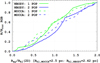 |
Fig. 1 Cumulative number distributions of RGB stars for the 1P (green) and 2P (blue) around 1.2 Gyr as a function of projected distance, normalised by the 2D half-light radius (Rhl). The solid line represents the N-body model (average of 33 snapshots) and the dashed line the MOCCA model (average of 5 snapshots). Snapshots span 1.18–1.22 Gyr. More details are provided in Fig. 4. |
2.2 Initial conditions
The initial conditions of the N-body model were chosen carefully, as large-scale direct N-body simulations are computationally expensive and time-consuming. Reproducing the cluster model presented in Giersz et al. (2025b) would require months of computation, mainly because of its very high primordial binary fraction (fb = 0.95) and the non-parallelised treatment of internal binary evolution (Huang et al. 2016). We therefore focused on reproducing the findings of Giersz et al. (2025b), namely the apparent 1P overconcentration in clusters close to dissolution, characterised by a small number of RGB stars and the presence of an active black hole subsystem (BHS). The selected N-body model dissolves on a much shorter timescale than a typical Milky Way GC, but it captures the essential physical processes relevant to the proposed mechanism.
The adopted initial conditions1 are as follows: initial number of particles N1P = 61 000 and N2P = 30 500, with a Kroupa (2001) initial mass function. The 1P stars were sampled in the mass range 0.08–150 M⊙, while the 2P stars were sampled between 0.08 and 20 M⊙. Both populations have metallicity Z1P = 0.001 and Z2P = 0.001, with binary fractions fb,1P = 0.1 and fb,2P = 0.1. These parameters correspond to an initial cluster mass of M(0) = 56 953.8 M⊙. The cluster was placed at a Galactocentric distance of RG = 2 kpc in a point-mass Galactic potential with MG = 2.25 × 10¹⁰ M⊙. The ratio of half-mass radii is Rh,2P/Rh,1P = 0.1. The two populations are initially in virial equilibrium, with the 1P component slightly tidally under-filled (Rtid = 18.9 pc). The initial King model (King 1966) concentration parameters were W0 = 3.0 for 1P and W0 = 7.0 for 2P. The initial conditions were generated using the publicly available McLuster2 code (Küpper et al. 2011; Leveque et al. 2022).
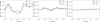 |
Fig. 2 Time evolution of the A+ parameter for different types of stars and for the X–Y projection of 3D snapshots. Left: RGB stars. Middle: evolved luminous stars. Right: MS stars. The red, green, and blue lines are averaged over 9, 17, and 33 snapshots, respectively. |
 |
Fig. 3 Time evolution of the number of RGB stars in the 1P, 2P, and total population for different projections of the 3D snapshots. Left: X–Y projection. Middle: X–Z projection. Right: Y–Z projection. The red, green, and blue lines correspond to averages over 9, 17, and 33 snapshots centred on the selected time, respectively. |
3 Results
Following the approach presented in Leitinger et al. (2023), we used the A+ parameter (Alessandrini et al. 2016; Dalessandro et al. 2018; Dalessandro et al. 2019) to assess the degree of spatial mixing between the 1P and the 2P. At 1.2 Gyr we have N1P = 9021 and N2P = 7206. As an illustration of the A+ parameter calculation, we show in Fig. 1 the cumulative projected distributions of RGB stars for both stellar populations of the N-body and MOCCA simulations. Both distributions are normalised by their numbers and their respective half-light radii. The total number of RGB stars at the reference time 1.2 Gyr is small, NRGB = 22 (see Fig. 3), so we collected data from snapshots between 1.18 and 1.22 Gyr and averaged the number distribution at 1.2 Gyr over a short time window. The MOCCA model has 5 snapshots, while the N-body model has 33 snapshots. The purpose of combining snapshots is not to increase the number of independent RGB stars, but to smooth the A+ measurement using a short time-smoothing window.
Figure 3 shows the time evolution of the RGB-star counts in the 1P and 2P for projections of the 3 D data onto the Galactic coordinate planes (X–Y, X–Z, and Y–Z). As expected, the RGB-star counts in each population are independent of projection direction and therefore show no systematic variation with projection. The number of RGB stars per snapshot is consistent and does not depend on the number of snapshots included in the averaging. The time steps are 0.116 Myr and 10 Myr for the NBODY6++GPU and MOCCA simulations, respectively.
In Fig. 4, in the left panel, the data show the cumulative relative number distribution of RGB stars in both populations. Each line in the plot shows the individual cumulative distribution of RGB stars for the 33 separate snapshots inside a time interval of ±2 Myr. The distribution fluctuates significantly between individual snapshots, making it extremely hard to determine the real A+. The relative cumulative distribution changes from snapshot to snapshot reflect the RGB stars’ physical movement inside the cluster, as shown in the right panel.
In Fig. 4, in the right panel, we present the particle dynamical orbits (for the eight RGB stars of the 2P) around 1.2 Gyr. We see the projected orbits during the dynamical orbital evolution of these RGB stars inside the cluster. The coordinates of the RGB stars in these 33 snapshots change significantly, so the combination of these 33 snapshots into one ‘merged’ system better represents the dynamical stage of the whole N-body system and the particle distribution.
Figure 1 shows that both models predict the 1P RGB population to be more centrally concentrated than the 2P RGB population. Taking into account the fact that we are comparing two simulations done with two different codes, the agreement between the 2D projected mass distributions of RGB stars for the two models is very good. Small differences in the curves reflect the stochastic spatial distribution of the small RGB sample and the different time averaging of snapshots, since MOCCA averages over a longer interval than the N-body results; therefore, identical shapes are not expected. The A+ parameters are 0.15 and 0.12 for the NBODY6++GPU and MOCCA models, respectively, at 1.2 Gyr.
The time evolution of the A+ parameter for different types of stars and for the X − Y projection (in the Galactic coordinate system) of 3D snapshots is presented in Fig. 2. The time range shown in the figure is from 0.8 to 1.25 Gyr. In the three panels, we show the time evolution for the different types of stars: RGB stars, evolved luminous stars (from the Hertzsprung gap to the helium giant branch), and main sequence (MS) stars. Each line presented in the figures was calculated by averaging a different number of snapshots. Each curve was computed using a sliding average over a window of snapshots centred on the reference time: 9 (±4), 17 (±8), or 33 (±16) snapshots.
Generally, each of the three averages gives a more or less consistent result for MS stars (right panel) and other types of luminous stars (middle panel). For the most interesting case of RGB stars (left panel), the snapshot averaging gives slightly different results depending on the time, with a spread of at most about 0.1. The spread is much smaller than the variation in the A+ parameter itself. Changes in the sign of the A+ parameter occur on a timescale of about 0.15 Gyr (much longer than the averaging time), indicating a strong time variability. On short timescales, the 1P becomes overconcentrated relative to the 2P and then quickly returns to a less concentrated state. The 1P overconcentration is a transient feature and confirms the findings of Giersz et al. (2025b).
The Giersz et al. (2025b) conclusions are further confirmed by the time evolution of the A+ parameter for MS and luminous evolved stars. No significant variation is seen in the A+ parameter, which remains close to 0. Both populations are fully mixed for MS and evolved luminous stars.
In Fig. 5, we show the evolution of the A+ parameter for different projections of the 3D snapshots onto the X–Y, X − Z, and Y − Z planes. The behaviour of A+ differs between projections, although the amplitude of the fluctuations remains comparable. At 1.2 Gyr, A+ is positive for the X–Y and Y–Z projections, while it is close to zero for the X–Z projection. This indicates that the inferred spatial distribution of RGB stars depends on the viewing direction, suggesting a non-spherical distribution of RGB stars. A weak dependence of A+ on the number of averaged snapshots is also present. The statistical fluctuations associated with different averaging windows are at the level of ±0.05–0.1, which is significantly lower than the intrinsic variations in A+ occurring over time intervals of 0.1–0.15 Gyr. This confirms that the transient behaviour of A+ reflects genuine changes in the global spatial distribution of RGB stars rather than artefacts of snapshot averaging.
Further confirmation of the transient feature of the overconcentration of the 1P RGB stars compared to the 2P RGB stars is provided by Fig. 5, in which the evolution of the A+ parameter is presented for different projections of the 3D snapshots: X–Y, X–Z, and Y–Z projections. We see that the A+ parameter shows similar strong variations and a transient character for all projections. The transient overconcentration of 1P RGB stars is not driven by projection effects but instead reflects the time evolution of the spatial distributions of RGB stars in the 1P and 2P.
In Fig. 6, we show the evolution of the cluster mass normalised to its initial value, together with the ratio of the BHS mass to the current cluster mass. This figure illustrates the key cluster state associated with the transient behaviour of the A+ parameter. When the cluster mass decreases to ~0.1 of its initial value and the BHS mass reaches ~0.05 of the current cluster mass, the number of RGB stars becomes very small. In this regime, stochastic fluctuations in their spatial distribution and strong dynamical interactions with the BHS drive the transient variations in A+. This behaviour is fully consistent with the findings of Giersz et al. (2025b).
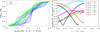 |
Fig. 4 Left: collection of the relative cumulative RGB star distribution for 1P and 2P stars for all 33 snapshots around 1.2 Gyr. Here we use for each snapshot its own half-light radius. These radii vary between 2.46 and 2.38 pc. Right: individual RGB stars’ projected coordinates inside the cluster. |
 |
Fig. 5 Time evolution of the A+ parameter for RGB stars for projections of the 3D snapshots onto the X–Y, X–Z, and Y–Z planes (left to right). The red, green, and blue lines show averages over 9, 17, and 33 snapshots, respectively. |
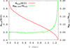 |
Fig. 6 NBODY6++GPU evolution of the cluster mass normalised to its initial value, M(0) = 56 953.8 M⊙ (red line), and of the BHS mass normalised to the current cluster mass (green line). |
4 Conclusions
We confirm the results of Giersz et al. (2025b), showing that when the analysis is based on RGB stars, the 1P can appear more centrally concentrated than the 2P at radii of a few half-light radii. Using direct N-body simulations tailored to reproduce the dynamical regime relevant to the proposed mechanism, we demonstrate that this apparent inversion is a transient feature and depends strongly on the adopted stellar tracers.
This effect is particularly relevant for GCs with present-day masses of a few times 105 M⊙, which have retained only ~10% of their initial mass and host an active BHS. In such systems, small-number statistics and strong dynamical interactions can significantly influence the spatial distribution of RGB stars, potentially leading to biased inferences about the global MSP structure when observations are restricted to this tracer population. To capture these processes while maintaining a feasible computational cost, we adopted a reduced-N model with an accelerated evolutionary timescale. Despite these simplifications, the simulations reproduce the key evolutionary behaviour of the reference MOCCA model. In line with Giersz et al. (2025b), the simulated cluster hosts an active BHS and is close to dissolution, with black holes contributing ~8% of the cluster mass when only ~10% of the initial mass remains, as seen in Fig. 6.
Figure 2 shows that the A+ parameter derived from RGB stars varies strongly over time, ranging between −0.3 and 0.4 over ~0.45 Gyr. In contrast, for evolved luminous stars (excluding compact remnants), A+ remains close to zero, indicating a near-complete mixing of the populations. When computed using only MS stars, the evolution follows the expected monotonic trend towards spatial mixing. The MOCCA simulation exhibits a comparable transient signal near 1.2 Gyr, with A+ ≃ 0.12, in close agreement with the NBODY6++GPU result (A+ ≃ 0.15), providing an independent validation of the Monte Carlo interpretation.
To further investigate the origin of the RGB trends discussed above and the cumulative number distributions shown in Fig. 1, we examined the escape properties of stars that would have evolved into RGB stars at 1.2 Gyr. In particular, we selected stars with initial masses in the range 1.71–1.74 M⊙ and identified those that escaped the cluster prior to this time. In Fig. 7, we show the cumulative distributions of their initial radial positions for the two populations, considering only escapers with securely identified population tags. As seen, the majority of 2P escapers originate from the innermost regions of the cluster, whereas 1P escapers are drawn from a much broader radial range. This demonstrates that centrally concentrated 2P RGB progenitors are preferentially removed through dynamical interactions in the cluster core, consistent with the behaviour shown in Fig. 3 of Giersz et al. (2025b). We also note that the number of escaped RGB progenitors is comparable to the number of such stars remaining in the cluster at 1.2 Gyr, indicating that this depletion is dynamically significant. We note that the number of identified 2P escapers should be regarded as a lower limit since a fraction of escapers cannot be unambiguously assigned to a given population. Nevertheless, the trend remains clear when considering only securely identified objects.
A similar role of dynamical interactions in removing centrally concentrated 2P stars from the cluster centre has recently been identified by Pavlík et al. (2025), who investigated spatial mixing driven by binary–single scattering with direct N-body simulations. Although their models do not show an inversion of the cumulative profiles, enriched stars are preferentially scattered to larger radii through binary–single encounters. The absence of inversion likely reflects the lack of strong mass loss and the near-dissolution evolution in their clusters. Taken together, these results suggest that while dynamical scattering can significantly modify MSP radial structure, the emergence of an apparent inversion requires clusters to have lost a substantial fraction of their initial mass. In this context, GCs such as NGC 3201 and NGC 6101, where 1P RGB stars are observed to be spatially over-concentrated, provide an interesting comparison. While these systems are inferred to have relatively high present-day mass fractions (e.g. Baumgardt & Makino 2003; Leitinger et al. 2023), such estimates rely on simplified assumptions about their orbital history and tidal environment (see the discussion in Giersz et al. 2025b) and may therefore be uncertain.
Projection-dependent variations in the inferred A+ evolution further demonstrate the sensitivity of cumulative diagnostics to sampling effects and viewing geometry. While these fluctuations do not alter the qualitative conclusion regarding the transient nature of RGB-based segregation, they highlight the importance of using multiple complementary diagnostics when interpreting spatial distributions. This is particularly relevant in light of recent observational work showing that MSPs have a complex and sometimes non-monotonic radial behaviour (e.g. Cadelano et al. 2024; Mehta et al. 2025), and that cumulative metrics alone may not fully capture underlying structural features. Our results, therefore, do not imply that enriched populations are globally less concentrated than pristine ones, but rather that tracer selection and the dynamical state can produce apparent inversions in specific diagnostics. In this context, the transient behaviour identified here may represent a dynamical pathway contributing to the observational diversity reported in recent studies.
We conclude that analyses based solely on RGB tracers should be interpreted with caution and that complementary approaches that use larger and dynamically less biased samples, such as MS stars, are essential for a robust inference of MSP structure. Further observational tests of tracer-dependent segregation and comparisons with diagnostics beyond cumulative distributions would provide valuable constraints on MSP formation scenarios, including the AGB framework and alternatives.
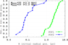 |
Fig. 7 Cumulative distributions of the initial radial positions of stars with initial masses in the range 1.71–1.74 M⊙ that would have evolved into RGB stars by 1.2 Gyr but escaped the cluster prior to this time. The green curve shows 1P escapers (N = 33 out of a total of 77 such stars in the initial model), and the blue curve shows 2P escapers (N = 15 out of a total of 40). The distributions demonstrate that 2P escapers originate predominantly from the inner regions of the cluster, whereas 1P escapers are drawn from a much broader radial range. This provides direct evidence that centrally concentrated 2P RGB progenitors are preferentially removed from the central parts of the cluster. |
Acknowledgements
The authors thank Sebastian Kamann for a very helpful and constructive comments. PB, MI, MS and OS thank the support from the special program of the Polish Academy of Sciences and the U.S. National Academy of Sciences under the Long-term program to support Ukrainian research teams, grant No. PAN.BFB.S.BWZ.329.022.2023. The authors appreciate the Polish high-performance computing infrastructure PLGrid (HPC Centre: ACK Cyfronet AGH – docs.hpc.cyfronet.pl) for providing Helios computer facilities and support within computational grant No. PLG/2026/019243. The authors also acknowledge the Gauss Centre for Supercomputing e.V. (www.gauss-centre.eu) for funding this project by providing computing time through the John von Neumann Institute for Computing (NIC) on the GCS Supercomputer JUWELS Booster and JUPITER Booster at Julich Supercomputing Centre (JSC), Germany. This material is based upon work supported by Tamkeen under the NYU Abu Dhabi Research Institute grant CASS. PB and MI thank Project No. BR24992759 “Development of the concept for the first Kazakhstani orbital cislunar telescope – Phase I”, financed by the Ministry of Science and Higher Education of the Republic of Kazakhstan. RS acknowledges NAOC International Cooperation Office for its support in 2023, 2024, and 2025. RS acknowledges Chinese Academy of Sciences President’s International Fellowship Initiative for Visiting Scientists (PIFI, grant No. 2026PVA0089), and the National Natural Science Foundation of China (NSFC) under grant No. 12473017. This research was supported in part by the grant NSF PHY-2309135 to the Kavli Institute for Theoretical Physics (KITP). RS and FFD acknowledge German Science Foundation (DFG) grant Sp 345/24-1. MG was supported by the Polish National Science Centre (NCN) through the grant 2021/41/B/ST9/01191. AA acknowledges that this research was funded in part by National Science Centre (NCN), Poland, grant No. 2024/55/D/ST9/02585.
References
- Alessandrini, E., Lanzoni, B., Ferraro, F. R., Miocchi, P., & Vesperini, E. 2016, ApJ, 833, 252 [NASA ADS] [CrossRef] [Google Scholar]
- Bastian, N., & Lardo, C. 2018, ARA&A, 56, 83 [Google Scholar]
- Baumgardt, H., & Makino, J. 2003, MNRAS, 340, 227 [NASA ADS] [CrossRef] [Google Scholar]
- Cadelano, M., Dalessandro, E., & Vesperini, E. 2024, A&A, 685, A158 [NASA ADS] [CrossRef] [EDP Sciences] [Google Scholar]
- Cordoni, G., Casagrande, L., Milone, A. P., et al. 2025, MNRAS, 537, 2342 [Google Scholar]
- Dalessandro, E., Cadelano, M., Vesperini, E., et al. 2018, ApJ, 859, 15 [NASA ADS] [CrossRef] [Google Scholar]
- Dalessandro, E., Cadelano, M., Vesperini, E., et al. 2019, ApJ, 884, L24 [Google Scholar]
- Dalessandro, E., Cadelano, M., Della Croce, A., et al. 2024, A&A, 691, A94 [NASA ADS] [CrossRef] [EDP Sciences] [Google Scholar]
- Decressin, T., Meynet, G., Charbonnel, C., Prantzos, N., & Ekström, S. 2007, A&A, 464, 1029 [NASA ADS] [CrossRef] [EDP Sciences] [Google Scholar]
- Denissenkov, P. A., & Hartwick, F. D. A. 2014, MNRAS, 437, L21 [Google Scholar]
- D’Ercole, A., Vesperini, E., D’Antona, F., McMillan, S. L. W., & Recchi, S. 2008, MNRAS, 391, 825 [CrossRef] [Google Scholar]
- Fregeau, J. M., & Rasio, F. A. 2007, ApJ, 658, 1047 [Google Scholar]
- Fregeau, J. M., Cheung, P., Portegies Zwart, S. F., & Rasio, F. A. 2004, MNRAS, 352, 1 [CrossRef] [Google Scholar]
- Geller, A. M., Leigh, N. W. C., Giersz, M., Kremer, K., & Rasio, F. A. 2019, ApJ, 872, 165 [NASA ADS] [CrossRef] [Google Scholar]
- Giersz, M. 1998, MNRAS, 298, 1239 [NASA ADS] [CrossRef] [Google Scholar]
- Giersz, M., Heggie, D. C., & Hurley, J. R. 2008, MNRAS, 388, 429 [Google Scholar]
- Giersz, M., Heggie, D. C., Hurley, J. R., & Hypki, A. 2013, MNRAS, 431, 2184 [NASA ADS] [CrossRef] [Google Scholar]
- Giersz, M., Askar, A., Hypki, A., et al. 2025a, A&A, 699, A76 [NASA ADS] [CrossRef] [EDP Sciences] [Google Scholar]
- Giersz, M., Askar, A., Hypki, A., et al. 2025b, A&A, 698, L11 [NASA ADS] [CrossRef] [EDP Sciences] [Google Scholar]
- Gratton, R., Bragaglia, A., Carretta, E., et al. 2019, A&A Rev., 27, 8 [Google Scholar]
- Hénon, M. H. 1971, Ap&SS, 14, 151 [Google Scholar]
- Huang, S.-Y., Spurzem, R., & Berczik, P. 2016, Res. Astron. Astrophys., 16, 11 [Google Scholar]
- Hypki, A., & Giersz, M. 2013, MNRAS, 429, 1221 [NASA ADS] [CrossRef] [Google Scholar]
- Hypki, A., Giersz, M., Hong, J., et al. 2022, MNRAS, 517, 4768 [NASA ADS] [CrossRef] [Google Scholar]
- Hypki, A., Vesperini, E., Giersz, M., et al. 2025, A&A, 693, A41 [NASA ADS] [CrossRef] [EDP Sciences] [Google Scholar]
- Kamann, S., Dalessandro, E., Bastian, N., et al. 2020a, MNRAS, 492, 966 [NASA ADS] [CrossRef] [Google Scholar]
- Kamann, S., Giesers, B., Bastian, N., et al. 2020b, A&A, 635, A65 [Google Scholar]
- Kamlah, A. W. H., Leveque, A., Spurzem, R., et al. 2022, MNRAS, 511, 4060 [NASA ADS] [CrossRef] [Google Scholar]
- King, I. R. 1966, AJ, 71, 64 [Google Scholar]
- Kroupa, P. 2001, MNRAS, 322, 231 [NASA ADS] [CrossRef] [Google Scholar]
- Küpper, A. H. W., Maschberger, T., Kroupa, P., & Baumgardt, H. 2011, MNRAS, 417, 2300 [Google Scholar]
- Kustaanheimo, P., & Stiefel, E. 1965, J. Reine Angew. Math., 218, 204 [Google Scholar]
- Leitinger, E., Baumgardt, H., Cabrera-Ziri, I., Hilker, M., & Pancino, E. 2023, MNRAS, 520, 1456 [NASA ADS] [CrossRef] [Google Scholar]
- Leitinger, E. I., Baumgardt, H., Cabrera-Ziri, I., et al. 2025, A&A, 694, A184 [Google Scholar]
- Leveque, A., Giersz, M., Banerjee, S., et al. 2022, MNRAS, 514, 5739 [NASA ADS] [CrossRef] [Google Scholar]
- Li, Z.-M., & Spurzem, R. 2026, Res. Astron. Astrophys., 26, 015009 [Google Scholar]
- Libralato, M., Vesperini, E., Bellini, A., et al. 2023, ApJ, 944, 58 [CrossRef] [Google Scholar]
- Madrid, J. P., Leigh, N. W. C., Hurley, J. R., & Giersz, M. 2017, MNRAS, 470, 1729 [NASA ADS] [CrossRef] [Google Scholar]
- Mehta, V. J., Milone, A. P., Casagrande, L., et al. 2025, MNRAS, 536, 1077 [Google Scholar]
- Milone, A. P., & Marino, A. F. 2022, Universe, 8, 359 [NASA ADS] [CrossRef] [Google Scholar]
- Nitadori, K., & Aarseth, S. J. 2012, MNRAS, 424, 545 [NASA ADS] [CrossRef] [Google Scholar]
- Pavlík, V., Davies, M. B., Leitinger, E. I., et al. 2025, A&A, 703, A157 [NASA ADS] [CrossRef] [EDP Sciences] [Google Scholar]
- Renzini, A., D’Antona, F., Cassisi, S., et al. 2015, MNRAS, 454, 4197 [Google Scholar]
- Rizzuto, F. P., Naab, T., Spurzem, R., et al. 2021, MNRAS, 501, 5257 [NASA ADS] [CrossRef] [Google Scholar]
- Spurzem, R., & Kamlah, A. 2023, Liv. Rev. Computat. Astrophys., 9, 3 [Google Scholar]
- Stodółkiewicz, J. S. 1982, Acta Astron., 32, 63 [Google Scholar]
- Ventura, P., D’Antona, F., Mazzitelli, I., & Gratton, R. 2001, ApJ, 550, L65 [CrossRef] [Google Scholar]
- Ventura, P., Di Criscienzo, M., Carini, R., & D’Antona, F. 2013, MNRAS, 431, 3642 [Google Scholar]
- Vergara, M. C., Askar, A., Kamlah, A. W. H., et al. 2025, A&A, 704, A321 [NASA ADS] [CrossRef] [EDP Sciences] [Google Scholar]
- Wang, L., Spurzem, R., Aarseth, S., et al. 2015, MNRAS, 450, 4070 [NASA ADS] [CrossRef] [Google Scholar]
- Wang, L., Spurzem, R., Aarseth, S., et al. 2016, MNRAS, 458, 1450 [Google Scholar]
Initial model and snapshot data are available at https://zenodo.org/records/20070757
All Figures
|
Fig. 1 Cumulative number distributions of RGB stars for the 1P (green) and 2P (blue) around 1.2 Gyr as a function of projected distance, normalised by the 2D half-light radius (Rhl). The solid line represents the N-body model (average of 33 snapshots) and the dashed line the MOCCA model (average of 5 snapshots). Snapshots span 1.18–1.22 Gyr. More details are provided in Fig. 4. |
| In the text | |
|
Fig. 2 Time evolution of the A+ parameter for different types of stars and for the X–Y projection of 3D snapshots. Left: RGB stars. Middle: evolved luminous stars. Right: MS stars. The red, green, and blue lines are averaged over 9, 17, and 33 snapshots, respectively. |
| In the text | |
|
Fig. 3 Time evolution of the number of RGB stars in the 1P, 2P, and total population for different projections of the 3D snapshots. Left: X–Y projection. Middle: X–Z projection. Right: Y–Z projection. The red, green, and blue lines correspond to averages over 9, 17, and 33 snapshots centred on the selected time, respectively. |
| In the text | |
|
Fig. 4 Left: collection of the relative cumulative RGB star distribution for 1P and 2P stars for all 33 snapshots around 1.2 Gyr. Here we use for each snapshot its own half-light radius. These radii vary between 2.46 and 2.38 pc. Right: individual RGB stars’ projected coordinates inside the cluster. |
| In the text | |
|
Fig. 5 Time evolution of the A+ parameter for RGB stars for projections of the 3D snapshots onto the X–Y, X–Z, and Y–Z planes (left to right). The red, green, and blue lines show averages over 9, 17, and 33 snapshots, respectively. |
| In the text | |
|
Fig. 6 NBODY6++GPU evolution of the cluster mass normalised to its initial value, M(0) = 56 953.8 M⊙ (red line), and of the BHS mass normalised to the current cluster mass (green line). |
| In the text | |
|
Fig. 7 Cumulative distributions of the initial radial positions of stars with initial masses in the range 1.71–1.74 M⊙ that would have evolved into RGB stars by 1.2 Gyr but escaped the cluster prior to this time. The green curve shows 1P escapers (N = 33 out of a total of 77 such stars in the initial model), and the blue curve shows 2P escapers (N = 15 out of a total of 40). The distributions demonstrate that 2P escapers originate predominantly from the inner regions of the cluster, whereas 1P escapers are drawn from a much broader radial range. This provides direct evidence that centrally concentrated 2P RGB progenitors are preferentially removed from the central parts of the cluster. |
| In the text | |
Current usage metrics show cumulative count of Article Views (full-text article views including HTML views, PDF and ePub downloads, according to the available data) and Abstracts Views on Vision4Press platform.
Data correspond to usage on the plateform after 2015. The current usage metrics is available 48-96 hours after online publication and is updated daily on week days.
Initial download of the metrics may take a while.