© ESO 2019

1 Introduction

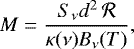
Estimating the mass of molecular dusty clumps is of great importance for a number of reasons, such as the determination of the clump mass function, the calculation of the virial parameter, the estimation of molecular abundances, among others. While various methods can be used for this purpose, the most common takes advantage of the fact that the spectral energy distribution (SED) of the continuum emission from a dusty homogeneous isothermal cloud can be approximated as a modified blackbody. In this case, the emission at sufficiently long wavelengths is optically thin and the integrated flux density can be easily expressed as a function of the mass and temperature of the dust. For a given gas-to-dust mass ratio, this allows us to derive the total mass of the cloud from the flux density, if the dust temperature and absorption coefficients are known. In practice, the cloud mass is evaluated as described in the pioneering study of Hildebrand (1983) and can be expressed as $$M=\frac{S_{\nu }{d}^2\mathcal{R}}{\kappa (\nu )B_{\nu }(T)},$$(1)

where S_ν is the flux density, d the distance to the cloud, B_ν the Planck function, T the dust temperature, κ the dust absorption coefficient per unit mass, and $\mathcal{R}$ the gas-to-dust mass ratio (see, e.g., Eq. (1) in Schuller et al. 2009).

While this simplified expression is perfectly adequate for most purposes, real life is much more complicated. Observations are currently performed at higher and higher frequencies, for example from space with the Herschel Space Observatory and from the ground with the Atacama Large Millimeter and submillimeter Array (ALMA), which is now operative up to 900 GHz. At such bands dust optical depth cannot be neglected a priori and should be considered when converting flux density into mass. In addition, compact molecular cores can be heated from the outside (by nearby luminous stars) or inside (by embedded forming stars), which generates temperature gradients that in turn break the assumption of isothermal clumps. Density gradients are likely present too, owing to collapse during the star formation process or other phenomena (e.g., expansion in molecular outflows).

Additional sources of uncertainty on the estimate of the mass are related to the error on the flux measurement, the distance of the source (often poorly known), and the value of the dust absorption coefficient, which depends on the properties of the dust grains (see, e.g., Ossenkopf & Henning 1994). The combination of all these errors may overcome the error caused by the assumptions of low optical depth and constant temperature. However, in some cases we are interested in quantities that do not depend on distance (e.g., the mass-to-luminosity ratio) or all the targets are located basically at the same distance (as in studies of the core mass function within the same molecular cloud), which makes the distance error irrelevant. In addition, for other quantities such as the virial parameter, it is important to determine whether the value lies above a given threshold. In cases like this, it is useful to improve on the accuracy of the estimated parameter as much as possible. Neglecting the opacity as well as the temperature and density gradients may lead to incorrect conclusions in these cases.

The goal of our study is to quantify the effects of large dust opacity and temperature and density gradients on the clump mass estimated with Eq. (1). In particular, in Sect. 2 we analyze the case of a spherically symmetric clump with temperature and density varying as power laws of the radius, in Sect. 3 we repeat the same exercise for a cylindrically symmetric clump, and in Sect. 4 we apply the corrections estimated via our method to data from the literature. Finally, the results are summarized in Sect. 5.

2 Flux density of spherical clump

We want tocalculate the integrated flux density emitted by the dust in a spherically symmetric clump. In our model the gas and dust are distributed between an inner radius R_i and an outer radius R_o, and the mass ratio between gas and dust $\mathcal{R}$ does not depend on the radius R. The dust temperature and density are expressed as $$\begin{array}{lll}T\hfill & =\hfill & T_{\text{o}}{\left(\frac{R}{R_{\text{o}}}\right)}^q,\hfill \\ \rho \hfill & =\hfill & {\rho }_{\text{o}}{\left(\frac{R}{R_{\text{o}}}\right)}^p,\hfill \end{array}$$

where T_o and ρ_o are the dust temperature and density at the outer radius. By definition, the gas density is equal to $\rho \mathcal{R}$.

2.1 Approximate analytical expression

As a first step, it is useful to calculate the expression of the integrated flux density in the optically thin and thick limits. In the latter only the photons emitted from the clump surface contribute to the observed flux, which is given by $$S_{\nu }=\frac{\pi B_{\nu }(T_{\text{o}})4{\text{piR}}_{\text{o}}^2}{4\pi d^2}={\Omega }_{\text{o}}{B}_{\nu }(T_{\text{o}}),$$(4)

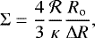
with ${\Omega }_{\text{o}}={\text{piR}}_{\text{o}}^2/d^2$ solid angle subtended by the clump. In practice, such a thick limit can hardly be reached at (sub)millimeter wavelengths. This can be seen by estimating the density needed to achieve a dust opacity of one in a thin surface layer of thickness (e.g., ΔR = 0.1 R_o). It is easy to show that the condition τ = κ ρ_o ΔR = 1 in the template case p = 0, and r_i = 0 can be rewritten as $$\Sigma =\frac{4}{3}\frac{\mathcal{R}}{\kappa }\frac{R_{\text{o}}}{\Delta R},$$(5)

where $\Sigma =(4/3)\mathcal{R}{\rho }_{\text{o}}{R}_{\text{o}}$ is the mean surface density of the clump. At 1 mm κ ≃ 1 cm² g⁻¹ (see Ossenkopf & Henning 1994) and for $\mathcal{R}=100$ we obtain Σ ≃ 10³ g cm⁻², as opposed to Σ≲1 g cm⁻² for typical molecular clumps.

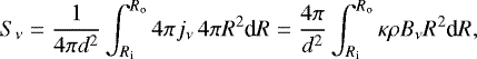
In the optically thin limit, instead, all photons emitted by the grains freely escape from the clump and S_ν is obtained from $$S_{\nu }=\frac{1}{4\pi d^2}{\displaystyle {\int }_{R_{\text{i}}}^{R_{\text{o}}}4}\pi j_{\nu }4\pi R^2\text{d}R=\frac{4\pi }{d^2}{\displaystyle {\int }_{R_{\text{i}}}^{R_{\text{o}}}\kappa }\rho B_{\nu }{R}^2\text{d}R,$$(6)

where j_ν is the dust emissivity and we make use of Kirchhoff’s law j_ν∕κ = B_ν(T). If hν ≪ kT (with k Boltzmann constant and h Planck constant), this equation can be rewritten using the Rayleigh-Jeans (hereafter RJ) approximation: $$\begin{array}{lll}{S}_{\nu }\hfill & \simeq \hfill & \frac{4\pi }{d^2}\kappa {\rho }_{\text{o}}\frac{2k{\nu }^2}{c^2}{T}_{\text{o}}{\displaystyle {\int }_{R_{\text{i}}}^{R_{\text{o}}}{R}^2}{\left(\frac{R}{R_{\text{o}}}\right)}^{q+p}\text{d}R\hfill \\ \hfill & =\hfill & \frac{4{\text{piR}}_{\text{o}}^3}{d^2}\kappa {\rho }_{\text{o}}\frac{2k{\nu }^2}{c^2}{T}_{\text{o}}{\displaystyle {\int }_{r_{\text{i}}}^1{r}^{q+p+2}}\text{d}r.\hfill \end{array}$$(7)

Here we define r = R∕R_o and r_i = R_i∕R_o.

We can relate the expression of S_ν to the mass of the clump M. The latter can be computed as $$M={\displaystyle {\int }_{R_{\text{i}}}^{R_{\text{o}}}\rho }\mathcal{R}4\pi R^2\text{\hspace{0.17em}d}R=4\pi R_{\text{o}}^3{\rho }_{\text{o}}\mathcal{R}{\displaystyle {\int }_{r_{\text{i}}}^1{r}^{p+2}}\text{\hspace{0.17em}d}r.$$(8)

From this expression and Eq. (7), we obtain $$S_{\nu }=\frac{\kappa M}{\mathcal{R}{d}^2}\frac{2k{\nu }^2}{c^2}{T}_{\text{o}}\frac{{\displaystyle {\int }_{r_{\text{i}}}^1{r}^{q+p+2}}\text{\hspace{0.17em}d}r}{{\displaystyle {\int }_{r_{\text{i}}}^1{r}^{p+2}}\text{\hspace{0.17em}d}r}=m\frac{2k{\nu }^2}{c^2}{T}_{\text{o}}F(r_{\text{i}};q,a),$$(9)

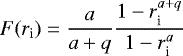
where we define 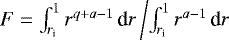$m=\kappa M/(\mathcal{R}{d}^2)$, a = p + 3, and $F={\displaystyle {\int }_{r_{\text{i}}}^1{r}^{q+a-1}}\text{\hspace{0.17em}d}r/{\displaystyle {\int }_{r_{\text{i}}}^1{r}^{a-1}}\text{\hspace{0.17em}d}r$. It is straightforward to demonstrate that function F takes the following values: $$F=\{\text{}\text{}\text{}\begin{array}{ccc}1& \iff & q=0,\\ \frac{r_{\text{i}}^q-1}{{\text{lnr}}_{\text{i}}^q}& \iff & q\ne 0, a=0,\\ \frac{{\text{lnr}}_{\text{i}}^{-q}}{r_{\text{i}}^{-q}-1}& \iff & q\ne 0, a\ne 0, a=-q,\\ \frac{a}{a+q}\frac{1-r_{\text{i}}^{a+q}}{1-r_{\text{i}}^a}& \iff & q\ne 0, a\ne 0, a\ne -q.\end{array}$$(10)

Finally, from Eq. (9) we obtain $$m=\frac{S_{\nu }}{\frac{2k{\nu }^2}{c^2}{T}_{\text{o}}}\frac{1}{F}$$(11)

or, equivalently, $$M=\frac{S_{\nu }{d}^2\mathcal{R}}{\kappa (\nu )\frac{2k{\nu }^2}{c^2}{T}_{\text{o}}}\frac{1}{F},$$(12)

which is analogous to Eq. (1) when the temperature and density gradients are taken into account. We note that these equations are valid only in the optically thin limit and under the RJ approximation.

It is interesting to discuss the transition between optically thin and optically thick regimes. The critical value of m for which such a transition occurs is obtained by equating the flux density from Eq. (4), in the RJ limit, to that from Eq. (9): $$m_{\text{c}}=\frac{{\Omega }_{\text{o}}}{F}.$$(13)

We note that the approximate relationship between S_ν and m is fully determined by Eqs. (4) and (13) because, once the optically thick flux and the critical value of m are fixed, the optically thin flux is also univocally established. This relationship can be used to study the dependence of S_ν on the various physical parameters.

The behavior of S_ν as a function of m is illustratedby the dashed curves in Fig. 1. In all panels the green curve corresponds to the approximate expressions of S_ν for a set of parameters arbitrarily chosen for illustrative purposes. These parameters are ν = 220 GHz, θ_o = R_o∕d = 1′′, r_i = 0.01, T_o = 50 K, q = −0.4, and p = −1.5 (i.e., a = 1.5). The blue and red curves are obtained by varying only one of these parameters, as detailed in each panel.

In particular, we observe that the optically thick flux from Eq. (4) and m_c are both proportional to Ω_o, but only the former depends on T_o. This implies that for increasing T_o the flux density increases, while the transition between the thin and thick regimes occurs approximately¹ at the same value of m. Instead, for increasing Ω_o the thick flux and m_c both increase by the same factor, while the optically thin flux remains the same (because Eq. (9) does not depend on R_o). Finally, it can be shown that function F increases with r_i if q > 0 and decreases if q < 0 (see Appendix A), which in turn implies that a variation of r_i affects only m_c and not the optically thick flux density.

The solid curves in the figure represent the flux density computed with the numerical model described in the next section, which properly takes into account the dust optical depth and does not assume the RJ approximation.

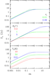Fig. 1 Template flux densities from a spherical dusty clump as a function of parameter m (see text).The curves are obtained for illustrative purposes from fiducial values of the input parameters: ν = 220 GHz, θo = Ro ∕d = 1′′, ri = 0.01, To = 50 K, q = −0.4, p = −1.5. In each panel only one of these parameters is changed, as indicated in the panel itself. Dashed curves represent the approximate analytical solutions given by Eq. (9), while solid curves are obtained from the numerical model described in Sect. 2.2.

2.2 Numerical solution

It is possible to obtain an exact semi-analytical expression of S_ν as a function of the clump mass only in the simple case q = 0 and p = 0. The result is given by Eq. (A.4) in Cesaroni et al. (2019), which with our notation takes the form $$\begin{array}{lll}{S}_{\nu }\hfill & =\hfill & {\Omega }_{\text{o}}{B}_{\nu }(T)\hfill \\ \hfill & \hfill & \times [1+\frac{2}{{\tau }_{\text{o}}}\left(\sqrt{1-r_{\text{i}}^2}{\text{e}}^{-{\tau }_{\text{o}}\sqrt{1-r_{\text{i}}^2}}+\frac{{\text{e}}^{-{\tau }_{\text{o}}\sqrt{1-r_{\text{i}}^2}}-1}{{\tau }_{\text{o}}}\right)\hfill \\ \hfill & \hfill & -{\displaystyle {\int }_0^{r_{\text{i}}^2}{\text{e}}^{-{\tau }_{\text{o}}\left(\sqrt{1-t}-\sqrt{r_{\text{i}}^2-t}\right)}}\text{d}t],\hfill \end{array}$$(14)

where τ_o = 2R_o κρ_o = 3m∕(2Ω_o).

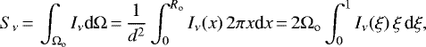
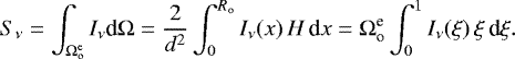
More ingeneral, the clump flux density can be estimated numerically as the integral of the brightness I_ν over the source solid angle, namely $$S_{\nu }={\displaystyle {\int }_{{\Omega }_{\text{o}}}{I}_{\nu }}\text{d}\Omega =\frac{1}{d^2}{\displaystyle {\int }_0^{R_{\text{o}}}{I}_{\nu }}(x)2\pi x\text{d}x=2{\Omega }_{\text{o}}{\displaystyle {\int }_0^1{I}_{\nu }}(\xi )\xi \text{\hspace{0.17em}d}\xi ,$$(15)

where x is the projected radius on the plane of the sky and we assume ξ = x∕R_o.

It is convenient to split the calculation of the brightness along an arbitrary line of sight (l.o.s.) through the clump into two parts, for positive and negative values of z, as $$\begin{array}{lll}{I}_{\nu }^0\hfill & =\hfill & I_{\nu }^{\text{BG}}{\text{e}}^{-{\displaystyle {\int }_{z_{\text{m}}}^{z_{\text{M}}}\kappa }\rho \text{d}z}+{\displaystyle {\int }_{z_{\text{m}}}^{z_{\text{M}}}{B}_{\nu }}{\text{e}}^{-{\displaystyle {\int }_{z_{\text{m}}}^z\kappa }\rho \text{d}{z}^{\prime }}\kappa \rho \text{\hspace{0.17em}d}z,\hfill \\ I_{\nu }\hfill & =\hfill & I_{\nu }^0{\text{e}}^{-{\displaystyle {\int }_{-z_{\text{M}}}^{-z_{\text{m}}}\kappa }\rho \text{d}z}+{\displaystyle {\int }_{-z_{\text{M}}}^{-z_{\text{m}}}{B}_{\nu }}{\text{e}}^{-{\displaystyle {\int }_{-z_{\text{M}}}^z\kappa }\rho \text{d}{z}^{\prime }}\kappa \rho \text{\hspace{0.17em}d}z,\hfill \end{array}$$

where z is the Cartesian coordinate along the l.o.s., $I_{\nu }^{\text{BG}}$ is the background brightness, the observer is located at z = −∞, and we define $$\begin{array}{lll}{z}_{\text{M}}\hfill & =\hfill & \sqrt{R_{\text{o}}^2-x^2}\hfill \\ z_{\text{m}}\hfill & =\hfill & \{\begin{array}{ccc}\sqrt{r_{\text{i}}^2-x^2}& \iff & 0\le x<r_{\text{i}}\\ 0& \iff & r_{\text{i}}\le x\le 1\end{array}\hfill \end{array}$$

(see Figs. 2a and b for a sketch of two representative l.o.s.).

In the following we focus on the solution of Eq. (16). The emergent brightness at z = −z_M given by Eq. (17) can be calculated via the same approach described below, once $I_{\nu }^0$ has been computed.

In order to obtain an approximate analytical solution of Eq. (16), we divide the part of the clump that contributes to the radiation along the given l.o.s. into a suitable number of shells N_S, and assume that in each shell the relevant physical parameters (density and temperature) are constant. Figure 2a shows a sketch of the shells for a generic l.o.s. with x > R_i, where only the dust between R = x and R = R_o contributes to the brightness, while Fig. 2b refers to the l.o.s. with 0 ≤ x < R_i, where the portion contributingto I_ν is the whole shell between R = R_i and R = R_o.

Under the previous approximation, Eq. (16) takes the form 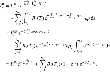$$\begin{array}{lll}{I}_{\nu }^0\hfill & =\hfill & I_{\nu }^{\text{BG}}{\text{e}}^{-{\sum }_{j=1}^{N_{\text{S}}}{\displaystyle {\int }_{z_{j-1}}^{z_j}\kappa }\rho \text{d}z}\hfill \\ \hfill & \hfill & +{\sum }_{j=1}^{N_{\text{S}}}{\displaystyle {\int }_{z_{j-1}}^{z_j}{B}_{\nu }}(T){\text{e}}^{-{\displaystyle {\int }_{z_{\text{m}}}^{z_{j-1}}\kappa }\rho \text{d}{z}^{\prime }-{\displaystyle {\int }_{z_{j-1}}^z\kappa }\rho \text{d}{z}^{\prime }}\kappa \rho \text{\hspace{0.17em}d}z\hfill \\ \hfill & \simeq \hfill & I_{\nu }^{\text{BG}}{\text{e}}^{-{\sum }_{j=1}^{N_{\text{S}}}\kappa {\rho }_j(z_j-z_{j-1})}\hfill \\ \hfill & \hfill & +{\sum }_{j=1}^{N_{\text{S}}}{B}_{\nu }(T_j){\text{e}}^{-{\sum }_{l=1}^{j-1}\kappa {\rho }_l(z_l-z_{l-1})}\kappa {\rho }_j{\displaystyle {\int }_{z_{j-1}}^{z_j}{\text{e}}^{-\kappa {\rho }_j(z-z_{j-1})}}\text{\hspace{0.17em}d}z\hfill \\ \hfill & =\hfill & I_{\nu }^{\text{BG}}{\text{e}}^{-{\sum }_{j=1}^{N_{\text{S}}}{\tau }_j}+{\sum }_{j=1}^{N_{\text{S}}}{B}_{\nu }(T_j)\left(1-{\text{e}}^{{\tau }_j}\right){\text{e}}^{-{\sum }_{l=1}^{j-1}{\tau }_l},\hfill \end{array}$$(20)

where we define z₀ = z_m, ${\sum }_{l=1}^0{\tau }_l=0$, τ_j = κρ_j(z_j − z_j−1), T_j = T(R_j), and ρ_j = ρ(R_j), with R_j outer radius of shell j. The opacity of shell j can be written as $$\begin{array}{lll}{\tau }_j\hfill & =\hfill & \kappa {\text{rhooR}}_{\text{o}}{r}_j^p\left(\sqrt{r_j^2-{\xi }^2}-\sqrt{r_{j-1}^2-{\xi }^2}\right)\hfill \\ \hfill & =\hfill & \frac{m}{4{\Omega }_{\text{o}}}\frac{r_j^{a-3}}{{\displaystyle {\int }_{r_{\text{i}}}^1{r}^{a-1}}\text{d}r}\left(\sqrt{r_j^2-{\xi }^2}-\sqrt{r_{j-1}^2-{\xi }^2}\right),\hfill \end{array}$$(21)

where we used Eq. (8).

Equation (20) can be easily implemented in a computer code as it is equivalent to iteratively solving the radiative transfer equation for each shell, using as input the output brightness of the previous shell crossed by the l.o.s.

The major problem with this approach is that a priori the density and/or temperature laws may be very steep close to the clump center if q and/or p are negative. Therefore, the thickness of the shells cannot be constant and must be adapted to the local value of the density and temperaturegradients. We propose a simple way to get around this problem.

In practice, what matters for our purposes is to estimate the flux density to a desired level of accuracy δS_ν. This meansthat we should divide the clump into a number of shells N_S, such that each of them does not contribute more than δS_ν to the total flux density. For a given l.o.s. with impact parameter x, the shells to be considered in Eq. (20) are those with R ≥ x if x > R_i, and R_i if x_i (see Fig. 2). Thus, the total flux density of interest for the integration along the given l.o.s. is that emitted between r = r₀ = max{ξ, r_i} and r = 1. This implies that a suitable value of N_S is given by $$N_{\text{S}}=\left[\frac{S_{\nu }(r_0;1)}{\delta S_{\nu }}\right]+1.$$(22)

Here the square brackets indicate the integer part of the argument and 1 is added to prevent the case N_S = 0. Moreover, we use the notation S_ν (r₁;r₂) to indicate the flux density emitted between two generic radii R₁ < R₂, which implies that S_ν(r_i;1) is the total flux density emitted by the clump.

The expression for the radius of a generic shell j is derived by imposing that each shell equally contributes with a fraction 1∕N_S to the total flux density S_ν(r₀;1), namely $$S_{\nu }(r_{j-1};r_j)=\frac{S_{\nu }(r_0;1)}{N_{\text{S}}}$$(23)

for any j = 1, …, N_S, under the assumption that r_j > r_j−1.

An approximate expression of S_ν(r₁;r₂), with r₁ < r₂, can be calculated in the optically thin and RJ limits from Eq. (7): $$S_{\nu }(r_1;r_2)\propto {\displaystyle {\int }_{r_1}^{r_2}{r}^{a+q-1}}\text{d}r=\{\text{}\text{}\begin{array}{ccc}\frac{r_2^{a+q}-r_1^{a+q}}{a+q}& \iff & a+q\ne 0,\\ \ln \left(\frac{r_2}{r_1}\right)& \iff & a+q=0.\end{array}$$(24)

Substituting this expression in Eq. (23), we obtain $$r_j^{a+q}=r_{j-1}^{a+q}+\frac{1-r_0^{a+q}}{N_{\text{S}}}$$(25)

for a + q≠0, and $$\ln r_j=\ln r_{j-1}-\frac{\ln r_0}{N_{\text{S}}}$$(26)

for a + q = 0. Since these expressions hold for any j, after some algebra we can finally write $$r_j=\{\text{}\text{}\begin{array}{ccc}{\left(r_0^{a+q}+j\frac{1-r_0^{a+q}}{N_{\text{S}}}\right)}^{\frac{1}{a+q}}& \iff & a+q\ne 0,\\ r_0^{1-\frac{j}{N_{\text{S}}}}& \iff & a+q=0.\end{array}$$(27)

Using Eq. (24) and setting δS_ν = εS_ν(r_i;1), we can also conveniently rewrite Eq. (22) as $$N_{\text{S}}=\left[\frac{S_{\nu }(r_0;1)}{\epsilon S_{\nu }(r_{\text{i}};1)}\right]+1=\left[\frac{1}{\epsilon }\frac{1-r_0^{a+q}}{1-r_{\text{i}}^{a+q}}\right]+1,$$(28)

where ε is the fraction of the total flux density emitted by the clump that we want to be contributed by each shell.

The solid curves in Fig. 1 are the numerical solutions obtained for the same set of parameters as the dashed curves with the same colour. For the sake of simplicity, in our calculations we assume $I_{\nu }^{\text{BG}}=0$. While, as expected, the numerical solution tends to converge to the corresponding approximate analytical solution for large and small values of m, the two may differ significantly for intermediate values of m. Moreover, some differences are also seen at small values of m due to the RJ approximation. In Sect. 2.3 we discuss all these features in more detail.

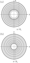Fig. 2 Sketch of two lines of sight (dashed lines) through a spherically symmetric clump (gray area) with impact parameter x, crossing (bottom panel) and not crossing (top panel) the central cavity of radius Ri (white central area). The thick circles denote the minimum and maximum radius of the region contributing to the brightness along the given l.o.s., while the thin circles are template annuli defined by Eq. (27), to be used for the numerical integration of the radiative transfer equation.

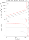Fig. 3 Panel a: m versus the total flux density of the clump. The red curves correspond to the case q = 0 and p = 0, while the black curves are for models allowing for temperature and density gradients. The dashed black curve has been obtained under the optically thin and RJ approximations from Eq. (11), whereas the dashed red curve is computed in the optically thin limit from Eq. (1). Panel b: mass ratios between all the curves in the top panel and the black solid curve.

2.3 Limits of the approximate analytical solutions

The main goal of our study is to establish how much the conversion from flux to mass can be affected by the usual assumption of constant dust density and temperature. Therefore, it is convenient to consider the inverse relationships with respect to those in Fig. 1 and plot the core mass as a function of the flux density. With this in mind, in Fig. 3a we show a plot of m, our proxy for the clump mass, versus S_ν. For illustrative purposes we considered an extreme case with ν = 600 GHz, θ_o = 10′′, T_o = 10 K, q = −0.5, p = −2, and r_i = 0.1, which emphasizes the drawbacks of using an approximate solution, as we show later. This set of parameters represents a typical clump, for example as observed in the Hi-GAL survey at 500 μm.

For the sake of comparison, in the same figure in addition to the numerical solution (black solid curve) we also plot the approximate analytical solution in the optically thin and RJ limits (black dashed curve) from Eq. (9), and the relationships (red curves) obtained under the commonly used assumption of constant density and temperature (equal to ρ_o and T_o, respectively). In particular, the red solid curve corresponds to the solution from Eq. (14), while the red dashed curve is computed in the optically thin limit from Eq. (1).

To emphasize the comparison between the various curves, in Fig. 3b we plot the ratio between the masses derived under the different approximations and that computed numerically. Clearly, at low fluxes the optically thin approximation is valid, as demonstrated by the excellent match between the solid and dashed red curves. However, for the same fluxes we see a significant difference between the solid and dashed black curves, due to the RJ approximation. At high fluxes the deviation with respect to the numerical solution is very prominent until the emission saturates due to the large opacity and a mass estimate cannot be obtained because of degeneracy of the solution.

We note that the above example is proposed only for illustrative purposes. More in general, it should be kept in mind that the deviation from the correct solution is sensitive to the input parameters of the model. This is especially true for the observing frequency and dust temperature, on which the goodness of the RJ approximation depends, and the steepness of the temperature and density gradients. The effect of such gradients can be seen by taking the ratio in the optically thin and RJ limits between the mass from Eq. (12) and that from Eq. (1). It is straightforward to demonstrate that such a ratio is equal to 1∕F, which depends only on r_i, q, and p or, equivalently,a. This result relies upon the assumption that the temperature used in Eq. (1) is T_o. Most studies derive the clump temperature from a modified blackbody fit to the SED of the source, which usually peaks in the far-IR where the emission is optically thick and traces the outer layers of the clump. Therefore, the temperature thus derived is very close to T_o.

Figure 4 shows the typical behavior of 1∕F as a function of r_i (see also Appendix A) for q = 0 (dotted line), q≠0, a≠ 0, a + q≠0 (blue curves), and in all the other cases (red curves). We see that a priori the presence of temperature and density gradients may lead to largely underestimating (if q > 0) or overestimating (if q < 0) the mass of the clump for sufficiently small values of r_i. Whether this occurs in practice and to what extent is discussed by means of a few examples in Sect. 4.

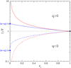Fig. 4 1∕F as a functionof ri. In addition to the trivial case q = 0 (dotted line), four representative cases are considered. Dashed and solid lines respectively correspond to q < 0 and q > 0, while blue indicates curves with a + q > 0 and a > 0 and red in all the other cases. The blue dots indicate the value ((a + q)∕a) of the corresponding curve for ri → 0+ and the black dot indicates the limit (1) of all curves for ri → 1−.

3 Flux density of cylindrical clump

Now, we compute the total flux density emerging from a cylindrically symmetric clump with height H, inner radius R_i, and outer radius R_o. This model might be more appropriate for some of the filamentary structures observed all over the Galaxy. Figure 5 shows the projection of the clump over the plane of the sky for a generic inclination angle ψ between the l.o.s. and the symmetry axis (ψ = 0 corresponds to face on). Temperature and density depend only on R through Eqs. (2) and (3).

3.1 Approximate analytical expression

As already done in Sect. 2, it is useful as a first step to consider the solution in the optically thin and thick limits.

3.1.1 Optically thick case

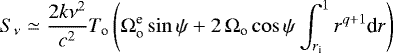
If the opacity is large, the flux is obtained by integrating the surface brightness over the solid angle subtended by the source. This is the sum of the integral over the light gray and the dark gray areas in Fig. 5. The latter has constant brightness equal to B_ν(T_o) and a surface comprised between two half ellipses described by the expressions $$\begin{array}{lll}{y}_1\hfill & =\hfill & \cos \psi \sqrt{R_{\text{o}}^2-x^2}-H\sin \psi ,\hfill \\ y_2\hfill & =\hfill & \cos \psi \sqrt{R_{\text{o}}^2-x^2},\hfill \end{array}$$

where x and y are Cartesian coordinates lying in the plane of the sky and oriented as shown in Fig. 5. The flux density of such a surface is hence given by 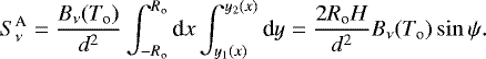$$S_{\nu }^{\text{A}}=\frac{B_{\nu }(T_{\text{o}})}{d^2}{\displaystyle {\int }_{-R_{\text{o}}}^{R_{\text{o}}}\text{d}}x{\displaystyle {\int }_{y_1(x)}^{y_2(x)}\text{d}}y=\frac{2R_{\text{o}}H}{d^2}{B}_{\nu }(T_{\text{o}})\sin \psi .$$(31)

The brightness over the light gray ellipse in Fig. 5 varies with R and the corresponding flux density is computed as $$\begin{array}{lll}{S}_{\nu }^{\text{B}}\hfill & =\hfill & \frac{4}{d^2}\left[{\displaystyle {\int }_0^{R_{\text{i}}}\text{d}}x{\displaystyle {\int }_{y_{\text{i}}(x)}^{y_{\text{o}}(x)}{B}_{\nu }}\text{\hspace{0.17em}d}y+{\displaystyle {\int }_{R_{\text{i}}}^{R_{\text{o}}}\text{d}}x{\displaystyle {\int }_0^{y_{\text{o}}(x)}{B}_{\nu }}\text{\hspace{0.17em}d}y\right]\hfill \\ \hfill & =\hfill & \frac{4\cos \psi }{d^2}[{\displaystyle {\int }_0^{R_{\text{i}}}\text{d}}X{\displaystyle {\int }_{Y_{\text{i}}(X)}^{Y_{\text{o}}(X)}{B}_{\nu }}(T(R))\text{\hspace{0.17em}d}Y\hfill \\ \hfill & \hfill & + {\displaystyle {\int }_{R_{\text{i}}}^{R_{\text{o}}}\text{d}}X{\displaystyle {\int }_0^{Y_{\text{o}}(X)}{B}_{\nu }}(T(R))\text{\hspace{0.17em}d}Y],\hfill \end{array}$$(32)

where $Y_{\text{i}}=\sqrt{R_{\text{i}}^2-x^2}$, $Y_{\text{o}}=\sqrt{R_{\text{o}}^2-x^2}$, y_i = Y_i cosψ, and y_o = Y_o cosψ, with X, Y Cartesian coordinates perpendicular to the cylinder axis, related to the x, y system through the expressions x = X, y = Y cosψ. In practice, Eq. (32) is the integral of B_ν over the face of the cylinder, multiplied by cosψ. This integral is more conveniently expressed in polar coordinates as $$\begin{array}{lll}{S}_{\nu }^{\text{B}}\hfill & =\hfill & \frac{4\cos \psi }{d^2}{\displaystyle {\int }_0^{\frac{\pi }{2}}\text{d}}\varphi {\displaystyle {\int }_{R_{\text{i}}}^{R_{\text{o}}}{B}_{\nu }}(T(R))R\text{\hspace{0.17em}d}R\hfill \\ \hfill & =\hfill & 2\cos \psi \frac{{\text{piR}}_{\text{o}}^2}{d^2}{\displaystyle {\int }_{r_{\text{i}}}^1{B}_{\nu }}(T(r))r\text{\hspace{0.17em}d}r.\hfill \end{array}$$(33)

The total flux density is hence given by the sum $S_{\nu }^{\text{A}}+S_{\nu }^{\text{B}}$, namely $$S_{\nu }={\Omega }_{\text{o}}^{\text{e}}\sin \psi B_{\nu }(T_{\text{o}})+2{\Omega }_{\text{o}}\cos \psi {\displaystyle {\int }_{r_{\text{i}}}^1{B}_{\nu }}(T(r))r\text{\hspace{0.17em}d}r,$$(34)

where ${\Omega }_{\text{o}}^{\text{e}}=2R_{\text{o}}H/d^2$ is the solid angle subtended by the clump seen edge on. In the RJ approximation we obtain $$S_{\nu }\simeq \frac{2k{\nu }^2}{c^2}{T}_{\text{o}}\left({\Omega }_{\text{o}}^{\text{e}}\sin \psi +2{\Omega }_{\text{o}}\cos \psi {\displaystyle {\int }_{r_{\text{i}}}^1{r}^{q+1}}\text{d}r\right)$$(35)

with $${\displaystyle {\int }_{r_{\text{i}}}^1{r}^{q+1}}\text{d}r=\{\text{}\text{}\begin{array}{ccc}\frac{1-r_{\text{i}}^{q+2}}{q+2}& \iff & q\ne -2,\\ -{\text{lnr}}_{\text{i}}& \iff & q=-2.\end{array}$$(36)

Fig. 5 Sketch of a cylindrical clump seen with an inclination angle ψ between the symmetry axis and the l.o.s. The figure represents the projection of the cylinder on the plane of the sky where the Cartesian system x, y lies. The radius and height of the cylinder are, respectively, Ro and H.

3.1.2 Optically thin case

In the optically thin limit, the flux density does not depend on the inclination angle because by definition the observer sees all the particles of the clump that contribute to the photon budget, independently of the shape and orientation of the clump. Therefore, the source luminosity is computed by integrating the emissivity over the clump volume $$\begin{array}{lll}{S}_{\nu }\hfill & =\hfill & \frac{H}{4\pi d^2}{\displaystyle {\int }_{R_{\text{i}}}^{R_{\text{o}}}4}\pi \kappa \rho (R)B_{\nu }(T(R))2\pi R\text{\hspace{0.17em}d}R\hfill \\ \hfill & \simeq \hfill & 2\frac{{\text{piR}}_{\text{o}}^{2}H}{d^2}{\rho }_{\text{o}}\kappa \frac{2k{\nu }^2}{c^2}{T}_{\text{o}}{\displaystyle {\int }_{r_{\text{i}}}^1{r}^{p+1}}\text{d}r,\hfill \end{array}$$

where we adopte the RJ approximation. Since the mass of the clump is equal to $$M={\displaystyle {\int }_{R_{\text{i}}}^{R_{\text{o}}}\rho }(R)\mathcal{R}2\pi RH\text{\hspace{0.17em}d}R=2\pi H{R}_{\text{o}}^2{\rho }_{\text{o}}\mathcal{R}{\displaystyle {\int }_{r_{\text{i}}}^1{r}^{p+1}}\text{d}r,$$(39)

we finally obtain 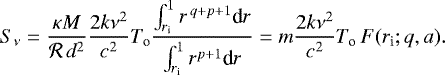$$S_{\nu }=\frac{\kappa M}{\mathcal{R}{d}^2}\frac{2k{\nu }^2}{c^2}{T}_{\text{o}}\frac{{\displaystyle {\int }_{r_{\text{i}}}^1{r}^{q+p+1}}\text{d}r}{{\displaystyle {\int }_{r_{\text{i}}}^1{r}^{p+1}}\text{d}r}=m\frac{2k{\nu }^2}{c^2}{T}_{\text{o}}F(r_{\text{i}};q,a).$$(40)

This expression is formally identical to Eq. (9), with the only difference that this time we define a = p + 2.

3.2 Numerical solution

Now we consider the general case with moderate opacity, which allows only a numerical solution. The calculation of the flux density for an arbitrary inclination angle is quite complicated and goes beyond the scope of the present study. Here we consider only the two extreme inclinations: face-on and edge-on.

3.2.1 Edge-on cylindrical clump

The calculation of S_ν is formally identical to that developed in Sect. 2.2, with the only difference that Eq. (15) must be replaced with $$S_{\nu }={\displaystyle {\int }_{{\Omega }_{\text{o}}^{\text{e}}}{I}_{\nu }}\text{d}\Omega =\frac{2}{d^2}{\displaystyle {\int }_0^{R_{\text{o}}}{I}_{\nu }}(x)H\text{\hspace{0.17em}d}x={\Omega }_{\text{o}}^{\text{e}}{\displaystyle {\int }_0^1{I}_{\nu }}(\xi )\xi \text{\hspace{0.17em}d}\xi .$$(41)

The brightness I_ν can be obtained by integrating along the l.o.s. exactly as described in Sect. 2.2, provided a = p + 3 is replaced with a = p + 2.

3.2.2 Face-on cylindrical clump

If the l.o.s. is parallel to the axis of the cylindrical clump, the flux density is computed from Eq. (15). The expression of the brightness I_ν is easily obtained because for a given x the density and temperature are constant along the l.o.s., hence $$I_{\nu }(\xi )=I_{\nu }^{\text{BG}}{\text{e}}^{-H\kappa {\rho }_{\text{o}}{\xi }^p}+B_{\nu }(T_{\text{o}}{\xi }^q)\left(1-{\text{e}}^{-H\kappa {\rho }_{\text{o}}{\xi }^p}\right),$$(42)

where we recall that we define ξ = x∕R_o.

4 Application to practical cases

As a test bed for the clump model previously described, we consider three examples taken from the literature. In two of these, the mass was estimated under the usual hypothesis of constant temperature and density and assuming optically thin emission.

4.1 Hot molecular core G31.41+0.31

As a first example, we consider the hot molecular core (HMC) G31.41+0.31, for which Beltrán et al. (2018; hereafter BEL18) derived a mass estimate from the 1.4 mm continuum emission imaged with ALMA. This case is especially suitable for our purposes because these authors also obtained an estimate of the temperature and density profiles as a function of the HMC radius. We adopt the same parameters used in their calculation, namely d = 7.9 kpc, R_o = 1.′′076, q = −0.77, p = −2, κ(217GHz) = 0.8, and $\mathcal{R}=100$. The total flux density of the core at ν = 217 GHz is S_ν = 3.1 Jy. The only unknown parameter is r_i, which BEL18 implicitly assumed equal to 0. In Fig. 6 we plot the values of the mass estimated in different ways as a function of r_i.

The mass obtained from our numerical solution (i.e., without any approximation) is represented by the black solid curve, while that derived under the optically thin and RJ approximations is shown as a dashed black curve. For the sake of comparison, we also mark with a blue dot the mass computed from Eq. (6) of BEL18. The resulting expression differs from our Eq. (12) by only a factor $(2/\sqrt{\pi })[\Gamma (-(p+q)/2)/\Gamma (-(p+q+1)/2)]\simeq 0.927$, because BEL18 calculated the brightness by integrating along the line of sight from − ∞ to + ∞, whereas we limit our integration to the sphere of radius R_o. Finally, we also show in the same figure the mass estimated from Eq. (14) (i.e., without the RJ approximation and assuming constant temperature and density) both with and without the optically thin assumption.

The largest difference between the various curves occurs for r_i = 0, not surprisingly because at small radii the effect of the temperature gradient is enhanced. Vice versa, for r_i close to 1, the temperature variation across the core is minimum and all curves converge towards the q = 0 solution corresponding to the red curves. In particular, the BEL18 solution for r_i = 0 is smaller than our numerical solution by a factor of ~2, whereas theconstant-temperature solutions predict a mass in excess by at least a factor ~2. It is also worth noting that the emission is partially thick in this HMC, as proved by the gap between the solid curves and the corresponding dashed curves.

The assumption r_i = 0 is obviously unrealistic, as the temperature and density laws must break down at some point close to the HMC center. A plausible hypothesis is that R_i is comparable to half the separation (0.′′1) between thetwo free–free sources detected by Cesaroni et al. (2010) close to the core center, which implies r_i ≃ 0.1 (see dotted line in Fig. 6). For this value the discrepancy among the different estimates of the mass is less prominent, but may still amount to 70%, which might not be negligible when comparing the core mass to other parameters such as the virial mass or the magnetic critical mass.

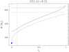Fig. 6 Mass of the HMC G31.41+0.31 as a function of ri. The input parameters are d = 7.9 kpc, Ro = 1.′′076, q = −0.77, p = −2, κ(217GHz) = 0.8, $\mathcal{R}=100$, S217 GHz = 3.1 Jy. The black lines are for q = −0.77 and p = −2, whereas the red lines correspond to q = 0 and p = 0. Both dashed lines are obtained in the optically thin limit, while the black dashed line also assumes the RJ approximation. The blue dot corresponds to the value of the mass computed by BEL18. The dotted vertical line marks a plausible upper limit for ri (see text).

4.2 Stability of massive star-forming clumps

Another useful test case for our model is represented by the sample of massive clumps observed by Fontani et al. (2002; hereafter FON02). In this case, as was done by BEL18, a direct estimate of the temperature and density gradients was obtained by FON02, who find q = −0.54 and p = −2.6. A puzzling result of their study is that the ratio of the clump masses to the corresponding virial masses is >1 (see their Fig. 6), which hints at some additional support that stabilizes the clumps, such as magnetic fields. However, the mass estimates made by FON02 were derived without taking into account the temperature and density gradients inside the clumps. Here we want to reconsider the problem by applying the appropriate corrections for these gradients.

At the time of publication, FON02 did not have a homogeneous data set available for the continuum emission of the clumps at (sub)millimeter wavelengths, and the authors had to rely upon a miscellany of observations obtained with various telescopes. Now the situation has changed and we can take advantage of Galaxy-wide surveys such as the APEX Telescope Large Area Survey of the Galaxy (ATLASGAL; Schuller et al. 2009), which covers almost all of the clumps studied by FON02.

We recalculated the clump masses using the flux densities at ν = 345 GHz from the ATLASGAL compact source catalogue (Urquhart et al. 2014; hereafter URQ14). For the sake of consistency with FON02, we adopt their distances, whereas we take the clump angular radius from URQ14 and T_o from Urquhart et al. (2018; hereafter URQ18). This last value was obtained from a modified blackbody fit to the SED and is hence a good approximation of the temperature at the surface of the clump, because the SEDs of these objects typically peak around ~100 μm where the emission is optically thick. We also adopt κ = 1.85 cm²g⁻¹ and $\mathcal{R}=100$, as in Schuller et al. (2009), and assume r_i = 0.01 based on the fact that the density gradient with p = −2.6 appears to hold on a range of radii spanning two orders of magnitude (see Fig. 10 of FON02).

The virial masses M_vir are recalculated, using the line widths ΔV from FON02and the new values of R_o and T_o from URQ14 and URQ18. In our estimates, unlike FON02, we take into account the correction to M_vir due to the density and temperature profiles, as detailed in Appendix B.

Figure 7 is the same as Fig. 6 of FON02 and shows the ratio between the clump mass and the corresponding virial mass for thedifferent sources. We also evaluated a mean error on this ratio taking into account that to a good approximation $M_{\text{clump}}/M_{\text{vir}}\propto S_{\nu }/[T_{\text{o}}{(\Delta V)}^2{\theta }_{\text{o}}]$ and assuming anuncertainty of 20% for all variables. The plot confirms that basically all clump masses are significantly greater than the corresponding virial masses if the clump mass is estimated with constant temperature and density. However, when the temperatureand density gradients are taken into account with our numerical model, almost all clumps become virialized. This result proves that the correction applied may be crucial for stability issues.

4.3 Masses of the ATLASGAL compact sources

As a last example, we discuss how temperature and density gradients could affect the estimates of the masses of the clumps identified in the ATLASGAL compact source catalogue by URQ18. In particular, we calculate the ratio of the mass computed with our method to that obtained by URQ18 from Eq. (1). For our estimates, θ_o and S_ν were taken from Table 1 of URQ14, T_o and d from Table 5 of URQ18, and we assume κ(345 GHz) = 1.85 cm²g⁻¹ and $\mathcal{R}=100$ for consistency with URQ18. We also set r_i = 0.01 for the reason explained in Sect. 4.2.

In Fig. 8 we plot the ratio of our numerical mass estimate, obtained as described in Sect. 2.2, to the mass computed by URQ18 (black dots), as a function of the latter ($M_{\text{o}}^{\text{thin}}$). The calculation is made for the fiducial values of q = −0.4, p = −1.5 (top panel) and for q = −0.54, p = −2.6, the values obtained by FON02 for their sample (bottom panel). The mean ratio is, respectively, 0.64 and 0.25, which represent a non-negligible correction for estimates of quantities such as the virial parameter.

It is useful to examine the separate contributions of opacity, RJ approximation, and temperature and density gradients to the correction factor. This can be done by trivially rewriting the mass ratio as $$\frac{M}{M_{\text{o}}^{\text{thin}}}=\left(\frac{M}{M^{\text{RJ}}}\frac{M_{\text{o}}^{\text{RJ-thin}}}{M_{\text{o}}^{\text{thin}}}\right) \frac{M^{\text{RJ}}}{M^{\text{RJ-thin}}} \frac{M^{\text{RJ-thin}}}{M_{\text{o}}^{\text{RJ-thin}}},$$(43)

where the indices “RJ” and “thin” indicate, respectively, that the mass is calculated in the RJ and in the optically thin approximation, while the subscript “o” means that the calculation is done for constant temperature and density (i.e., T =T_o and ρ = ρ_o).

On the right-hand side of Eq. (43), the term in parentheses is sensitive to the RJ approximation, the ratio M^RJ∕M^RJ-thin is related to the opacity of the clump, and $M^{\text{RJ-thin}}/M_{\text{o}}^{\text{RJ-thin}}=1/F$ is the correction for the temperature and density gradients. These three quantities are plotted in Fig. 8 as red dots (M^RJ∕M^RJ-thin), blue dots ($M{M}_{\text{o}}^{\text{RJ-thin}}/({\text{MrjM}}_{\text{o}}^{\text{thin}})$), and a green line ($M^{\text{RJ-thin}}/M_{\text{o}}^{\text{RJ-thin}}$).

We conclude that the most important correction is due to the gradients, although in a non-negligible number of clumps opacity may play an important role, provided the temperature and density gradients are sufficiently steep.

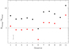Fig. 7 Same as Fig. 6 in FON02, where the clump masses are recomputed with our numerical solution using the temperature, radii, and flux densities from the ATLASGAL compact source catalogue, and the virial masses are corrected to take into account density and temperature gradients. The numbers on the x-axis identify the clumps according to the numbering of Table 1 of FON02. Black circles correspond to constant density and temperature, as assumed by FON02, whereas red squares are obtained adopting q = −0.54 and p = −2.6, consistent with the findings of FON02. The error bar in the bottom left corner indicates the typical uncertainty on the mass ratio.

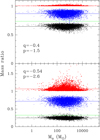Fig. 8 Ratio of the mass estimated with our numerical model to that computed by URQ18 for the compact sources identified in the ATLASGAL survey (black dots). The input parameters are taken from URQ18. For our estimates, we assumed two template cases: q = −0.4, p = −1.5 (top panel) and q = −0.54, p = −2.6 (bottom panel). The red and blue dots indicate, respectively, the contribution of opacity and RJ approximation to the mass ratio, with the horizontal lines denoting the corresponding mean values for the black dots (0.64 top panel; 0.25 bottom panel), red dots (1.01 top panel; 1.07 bottom panel), and blue dots (0.87 top panel; 0.72 bottom panel). The green line is the factor (0.74 top panel; 0.33 bottom panel) taking into account temperature and density gradients (see text for a detailed explanation).

5 Summary and conclusions

We estimated the continuum emission from a dusty clump with temperature and density gradients, assuming both spherical and cylindrical symmetry. While our toy model assumes power-law profiles for the physical parameters, it must be kept in mind that

real clumps are more complex structures where the temperature and density distributions are determined by heating and cooling processes and must obey the laws of fluidodynamics. Fragmentation and sub-clumpiness may also affect the observed flux densities, especially if coupled to large opacities. Finally, clumps are enshrouded in more extended lower density structures whose emission or absorption might affect the measured flux from the clump. All these issues go beyond the scope of our study, which is nonetheless useful to improve on the usual simplified assumption of homogeneous, optically thin clumps.

We provide the reader with approximate analytical expressions (summarized in Table 1) to calculate the flux density as a function of the clump mass and other relevant parameters and, conversely, to derive the mass from the measured flux in the optically thin and RJ limits. In addition, in Eqs. (20) and (27) we give an approximate solution to the radiative transfer equation to calculate the brightness along an arbitrary line of sight through the clump for any optical depth. Our approach overcomes the problem represented by possibly steep density and temperature gradients at small clump radii. The approximate solution is then used to evaluate the flux density of the core numerically.

Comparison between the numerical and approximate analytical solutions allows us to inspect the limits due to the optically thin, Rayleigh-Jeans, and constant density and temperature approximations. We conclude that in most cases the correction is about a factor of 2–3, although in some extreme cases characterized by unusually steep gradients and/or high frequencies, the error introduced by the above approximations can be larger. In order to illustrate all these effects, we applied our method to three practical examples taken from the literature, demonstrating that the correction to the clump mass may significantly affect the estimate of the clump stability.

Acknowledgements

It is a pleasure to thank Daniele Galli and Maite Beltrán for critically reading the manuscript and for the useful suggestions.

Appendix A Function F(r_i;q,a)

The purpose of this appendix is to study the behavior of F defined by Eq. (10) as a function of r_i, in the non-trivial case q≠0. In the following we consider three possible cases depending on the value of a and demonstrate that F always increases with r_i if q > 0, and decreases if q < 0.

A.1 Case a = 0

In this case $F(r_{\text{i}})=(r_{\text{i}}^q-1)/{\text{lnr}}_{\text{i}}^q$, which may be convenientlyre written as F′(y) = (y − 1)∕lny with $y=r_{\text{i}}^q$. The function is to be studied in the range 0 < r_i ≤ 1 or y> 0.

First of all we note that $$\underset{r_{\text{i}}\to 0^{+}}{\lim }F(r_{\text{i}})=\{\text{}\text{}\begin{array}{ccc}\underset{y\to 0^{+}}{\lim }\frac{-1}{\ln y}=0& \iff & q>0\\ \underset{y\to +\infty }{\lim }\frac{y}{\ln y}=\underset{t\to 0^{+}}{\lim }\frac{1}{-t\ln t}=+\infty & \iff & q<0\end{array}$$

and $$\underset{r_{\text{i}}\to 1^{-}}{\lim }F(r_{\text{i}})=\underset{y\to 1}{\lim }{F}^{\prime }(y)=\underset{t\to 0}{\lim }\frac{t}{\ln (1+t)}=1,$$

where we define t = y − 1. Furthermore, the derivative of F′(y) is equal to 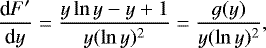$$\frac{\text{d}{F}^{\prime }}{\text{d}y}=\frac{y\ln y-y+1}{y{(\ln y)}^2}=\frac{g(y)}{y{(\ln y)}^2},$$(A.1)

whose sign is determined by the sign of g(y) = ylny − y + 1. Since g(1) = 0 and dg∕dy = lny > 0 ⇔ y > 1, we conclude that g has a minimum in y = 1, and thus g ≥ 0 for any y > 0. Consequently, dF′∕dy ≥ 0 and $\text{d}F/\text{d}{r}_{\text{i}}=q{r}_{\text{i}}^q(\text{d}{F}^{\prime }/\text{d}y)>0\iff q>0$.

A.2 Case a ≠ 0 and a = −q

The result inthis case is straightforward. Function $F(r_{\text{i}})={\text{lnr}}_{\text{i}}^a/(r_{\text{i}}^a-1)$ with a =−q is the inverse of that studied in Sect. A.1, and is thus increasing with r_i if and only if a < 0 (i.e., for q > 0).

A.3 Case a ≠ 0 and a ≠−q

In this case it is useful to rewrite the function $$F(r_{\text{i}})=\frac{a}{a+q}\frac{1-r_{\text{i}}^{a+q}}{1-r_{\text{i}}^a}$$(A.2)

assuming $y=r_{\text{i}}^a$ and b = (a + q)∕a, which gives $$F^{\prime }(y)=\frac{1}{b}\frac{1-y^b}{1-y}.$$(A.3)

For any value of a≠0, we find $$\underset{r_{\text{i}}\to 1^{-}}{\lim }F(r_{\text{i}})=\underset{y\to 1}{\lim }{F}^{\prime }(y)=\underset{t\to 0}{\lim }\frac{1}{b}\frac{1-{(1+t)}^b}{-t}=1.$$

The calculation of the value of F for r_i = 0 depends on the sign of a. We obtain for a > 0 $$\underset{r_{\text{i}}\to 0^{+}}{\lim }F(r_{\text{i}})=\underset{y\to 0^{+}}{\lim }{F}^{\prime }(y)=\{\text{}\text{}\text{}\begin{array}{ccc}\frac{1}{b}& \iff & b>0\\ +\infty & \iff & b<0\end{array}$$

and for a < 0 $$\underset{r_{\text{i}}\to 0^{+}}{\lim }F(r_{\text{i}})=\text{}\underset{y\to +\infty }{\lim }\text{}{F}^{\prime }(y)=\text{}\{\text{}\text{}\text{}\begin{array}{ccc}\underset{y\to +\infty }{\lim }\frac{1}{b}\frac{y^b}{y}=+\infty & \iff & b>1,\\ \underset{y\to +\infty }{\lim }\frac{1}{b}\frac{y^b}{y}=0& \iff & 0<b<1,\\ \underset{y\to +\infty }{\lim }\frac{1}{b}\frac{1}{y}=0& \iff & b<0.\end{array}$$

We notethat b = 0 and b = 1 are excluded because we are considering the case for a + q≠0 and q≠0.

In conclusion, $$\underset{r_{\text{i}}\to 0^{+}}{\lim }F(r_{\text{i}})=\{\text{}\text{}\text{}\begin{array}{ccc}0& \iff & a<0, q<0,\\ \frac{a}{a+q}& \iff & a>0, a+q>0,\\ +\infty & \iff & a<0, q>0 \text{or} a>0, a+q<0.\end{array}$$

The derivative of F is $\text{d}F/\text{d}{r}_{\text{i}}=a{r}_{\text{i}}^{a-1}\text{d}{F}^{\prime }/\text{d}y$, where $$\frac{\text{d}{F}^{\prime }}{\text{d}y}=\frac{1}{b}\frac{-b{y}^{b-1}(1-y)+1-y^b}{{(1-y)}^2}$$(A.4)

so that the sign of dF∕dr_i depends on ag(y)∕b, where we define g(y) = −by^b−1(1 − y) + 1 − y^b. We find that dg∕dy = b(b − 1)y^b−2(y − 1) ≥ 0 if y ≥ 1, for b(b − 1) > 0, and if y ≤ 1, for b(b − 1) < 0. This means that g has a minimum in y = 1 if b > 1 or b < 0, a maximum if 0 < b < 1. Consequently, for any y it is g ≥ 0 in the former case and g ≤ 0 in the latter, because in all cases g(1) = 0.

Based on the above, we find that g∕b > 0 ⇔ b > 1, so that dF∕dr_i ∝ ag∕b > 0 ⇔ a > 0, (a + q)∕a > 1 or a < 0, (a + q)a < 1. Both conditions are equivalent to q > 0. We concludethat F(r_i) is a growing function of r_i if and only if q > 0. Since F(1) = 1, this also implies that F ≥ 1 ⇔ q < 0.

Appendix B Virial mass with density and temperature gradients

We want to derive the expression of the virial mass of a spherically symmetric clump with temperature and density described by Eqs. (2) and (3). The virial theorem can be expressed as in Eqs. (8.4) and (8.5) in Dyson & Williams (1980), for example, namely $$3{\displaystyle \int P}\text{d}V={\displaystyle \int G}\frac{M(R)}{R}\text{d}M,$$(B.1)

where P is the gas pressure, V the volume, M(R) the mass inside radius R, G the gravitational constant, and we assume that the external pressure is null. Using our notation (see Sect. 2), M(R) is obtained by integrating Eq. (8) between R_i and R: 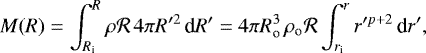$$M(R)={\displaystyle {\int }_{R_{\text{i}}}^R\rho }\mathcal{R}4\pi {R^{\prime }}^2\text{\hspace{0.17em}d}{R}^{\prime }=4\pi R_{\text{o}}^3{\rho }_{\text{o}}\mathcal{R}{\displaystyle {\int }_{r_{\text{i}}}^r{r^{\prime }}^{p+2}}\text{\hspace{0.17em}d}{r}^{\prime },$$(B.2)

which can be written as $$M(R)=M(R_{\text{o}})\frac{{\displaystyle {\int }_{r_{\text{i}}}^r{r^{\prime }}^{p+2}}\text{\hspace{0.17em}d}{r}^{\prime }}{{\displaystyle {\int }_{r_{\text{i}}}^1{r^{\prime }}^{p+2}}\text{\hspace{0.17em}d}{r}^{\prime }}.$$(B.3)

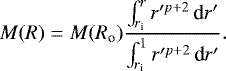
The gaspressure is $$P(R)=\mathcal{R}\rho (R)\left(\frac{kT(R)}{\mu }+\frac{{\sigma }_{\text{NT}}^2}{3}\right),$$(B.4)

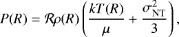
where μ is the mean mass per particle and σ_NT is the velocity dispersion due to microscopic non-thermal motions, which we assume are independent of R. The virial mass M_vir is the value of M(R_o) that satisfies Eq. (B.1), which takes the form $$\begin{array}{lll}\hfill & \hfill & {\displaystyle {\int }_{r_{\text{i}}}^1\left(3\mathcal{R}{\rho }_{\text{o}}\frac{k{T}_{\text{o}}}{\mu }{r}^{p+q}+\mathcal{R}{\rho }_{\text{o}}{\sigma }_{\text{NT}}^2{r}^p\right)}{R}_{\text{o}}^{3}4\pi r^2\text{\hspace{0.17em}d}r\hfill \\ \hfill & \hfill & ={\displaystyle {\int }_{r_{\text{i}}}^{1}G}{M}_{\text{vir}}\frac{{\displaystyle {\int }_{r_{\text{i}}}^r{r^{\prime }}^{p+2}}\text{\hspace{0.17em}d}{r}^{\prime }}{{\displaystyle {\int }_{r_{\text{i}}}^1{r^{\prime }}^{p+2}}\text{\hspace{0.17em}d}{r}^{\prime }}4\pi \mathcal{R}{\rho }_{\text{o}}{R}_{\text{o}}^2{r}^{p+1}\text{\hspace{0.17em}d}r.\hfill \end{array}$$(B.5)

The solution is $$\begin{array}{lll}{M}_{\text{vir}}\hfill & =\hfill & \frac{{\sigma }_{\text{NT}}^2{R}_{\text{o}}}{G}{\displaystyle {\int }_{r_{\text{i}}}^1{r}^{p+2}}\text{\hspace{0.17em}d}r\hfill \\ \hfill & \hfill & \times \frac{\eta {\displaystyle {\int }_{r_{\text{i}}}^1{r}^{p+q+2}}\text{\hspace{0.17em}d}r+{\displaystyle {\int }_{r_{\text{i}}}^1{r}^{p+2}}\text{\hspace{0.17em}d}r}{{\displaystyle {\int }_{r_{\text{i}}}^1\left({\displaystyle {\int }_{r_{\text{i}}}^r{r^{\prime }}^{p+2}}\text{\hspace{0.17em}d}{r}^{\prime }\right)}{r}^{p+1}\text{\hspace{0.17em}d}r},\hfill \end{array}$$(B.6)

where we define ${\sigma }_{\text{o}}^2=3k{T}_{\text{o}}/\mu$ and $\eta ={\sigma }_{\text{o}}^2/{\sigma }_{\text{NT}}^2$. Depending on the values of p and q the solution takes the following forms: $$\begin{array}{lll}{M}_{\text{vir}}\hfill & =\hfill & M_{\text{NT}}\hfill \\ \hfill & \hfill & \times \{\begin{array}{ccc}\left(\eta +1\right)\frac{r_{\text{i}}{\ln }^2{r}_{\text{i}}}{1+r_{\text{i}}{\text{lnr}}_{\text{i}}-r_{\text{i}}}& \iff & p=-3, q=0,\\ r_{\text{i}}{\text{lnr}}_{\text{i}}\frac{{\text{lnr}}_{\text{i}}-\eta \frac{1-r_{\text{i}}^q}{q}}{1+r_{\text{i}}{\text{lnr}}_{\text{i}}-r_{\text{i}}}& \iff & p=-3, q\ne 0,\\ \left(\frac{1-r_{\text{i}}^{p+3}}{p+3}-\eta {\text{lnr}}_{\text{i}}\right)\frac{1-r_{\text{i}}^{p+3}}{E(r_{\text{i}},p)}& \iff & p\ne -3, q=-p-3,\\ \left(\eta \frac{1-r_{\text{i}}^{p+q+3}}{p+q+3}+\frac{1-r_{\text{i}}^{p+3}}{p+3}\right)\frac{1-r_{\text{i}}^{p+3}}{E(r_{\text{i}},p)}& \iff & p\ne -3, q\ne -p-3,\end{array}\hfill \end{array}$$(B.7)

where $M_{\text{NT}}={\sigma }_{\text{NT}}^2{R}_{\text{o}}/G$ and

It is possible to demonstrate that if p ≤−5∕2 or q≤−p − 3, for r_i → 0⁺ no equilibrium configuration can be attained, because either the gravitational energy overwhelms the internal energy of the clump (M_vir → 0) or the opposite happens (M_vir → +∞). Vice versa, for p > −5∕2 and q > −p − 3 we find that $$\underset{r_{\text{i}}\to 0^{+}}{\lim }{M}_{\text{vir}}=M_{\text{NT}}(2p+5)\left(\frac{1}{p+3}+\frac{\eta }{p+q+3}\right),$$(B.9)

which for η = 0 (i.e., negligible thermal contribution to the internal energy) turns into Eq. (1) in MacLaren (1988)².

The mass M_NT can be conveniently expressed in useful units as $$M_{\text{NT}}=\frac{3{(\Delta V)}^2}{8\ln 2}\frac{R_{\text{o}}}{G}=125.8 M_{\odot } {[\Delta V(\text{mbox}km s{\$}^{-1}\$)]}^2{R}_{\text{o}}(\text{pc}),$$(B.10)

where the factor 3 takes into account that the observed line full width at half maximum, ΔV, is a measurement of the velocity dispersion along the l.o.s. (i.e., in one dimension).

The relevant parameters for the case discussed in Sect. 4.2 are p = −2.6, q = −0.54, and r_i = 0.01, which imply $M_{\text{vir}}{\text{simeqM}}_{\text{NT}}(1.496\eta +0.487)$, with $\eta \simeq 0.01647T_{\text{o}}(K)/[\Delta V(\text{mbox{}km s$. Here we assume μ = 2.8 m_H, with m_H the mass of the hydrogen atom.

References

All Tables

All Figures

Fig. 1 Template flux densities from a spherical dusty clump as a function of parameter m (see text).The curves are obtained for illustrative purposes from fiducial values of the input parameters: ν = 220 GHz, θo = Ro ∕d = 1′′, ri = 0.01, To = 50 K, q = −0.4, p = −1.5. In each panel only one of these parameters is changed, as indicated in the panel itself. Dashed curves represent the approximate analytical solutions given by Eq. (9), while solid curves are obtained from the numerical model described in Sect. 2.2.

In the text

Fig. 2 Sketch of two lines of sight (dashed lines) through a spherically symmetric clump (gray area) with impact parameter x, crossing (bottom panel) and not crossing (top panel) the central cavity of radius Ri (white central area). The thick circles denote the minimum and maximum radius of the region contributing to the brightness along the given l.o.s., while the thin circles are template annuli defined by Eq. (27), to be used for the numerical integration of the radiative transfer equation.

In the text

Fig. 3 Panel a: m versus the total flux density of the clump. The red curves correspond to the case q = 0 and p = 0, while the black curves are for models allowing for temperature and density gradients. The dashed black curve has been obtained under the optically thin and RJ approximations from Eq. (11), whereas the dashed red curve is computed in the optically thin limit from Eq. (1). Panel b: mass ratios between all the curves in the top panel and the black solid curve.

In the text

Fig. 4 1∕F as a functionof ri. In addition to the trivial case q = 0 (dotted line), four representative cases are considered. Dashed and solid lines respectively correspond to q < 0 and q > 0, while blue indicates curves with a + q > 0 and a > 0 and red in all the other cases. The blue dots indicate the value ((a + q)∕a) of the corresponding curve for ri → 0+ and the black dot indicates the limit (1) of all curves for ri → 1−.

In the text

	Fig. 5 Sketch of a cylindrical clump seen with an inclination angle ψ between the symmetry axis and the l.o.s. The figure represents the projection of the cylinder on the plane of the sky where the Cartesian system x, y lies. The radius and height of the cylinder are, respectively, Ro and H.
In the text

Fig. 6 Mass of the HMC G31.41+0.31 as a function of ri. The input parameters are d = 7.9 kpc, Ro = 1.′′076, q = −0.77, p = −2, κ(217GHz) = 0.8, $\mathcal{R}=100$, S217 GHz = 3.1 Jy. The black lines are for q = −0.77 and p = −2, whereas the red lines correspond to q = 0 and p = 0. Both dashed lines are obtained in the optically thin limit, while the black dashed line also assumes the RJ approximation. The blue dot corresponds to the value of the mass computed by BEL18. The dotted vertical line marks a plausible upper limit for ri (see text).

In the text

Fig. 7 Same as Fig. 6 in FON02, where the clump masses are recomputed with our numerical solution using the temperature, radii, and flux densities from the ATLASGAL compact source catalogue, and the virial masses are corrected to take into account density and temperature gradients. The numbers on the x-axis identify the clumps according to the numbering of Table 1 of FON02. Black circles correspond to constant density and temperature, as assumed by FON02, whereas red squares are obtained adopting q = −0.54 and p = −2.6, consistent with the findings of FON02. The error bar in the bottom left corner indicates the typical uncertainty on the mass ratio.

In the text

Fig. 8 Ratio of the mass estimated with our numerical model to that computed by URQ18 for the compact sources identified in the ATLASGAL survey (black dots). The input parameters are taken from URQ18. For our estimates, we assumed two template cases: q = −0.4, p = −1.5 (top panel) and q = −0.54, p = −2.6 (bottom panel). The red and blue dots indicate, respectively, the contribution of opacity and RJ approximation to the mass ratio, with the horizontal lines denoting the corresponding mean values for the black dots (0.64 top panel; 0.25 bottom panel), red dots (1.01 top panel; 1.07 bottom panel), and blue dots (0.87 top panel; 0.72 bottom panel). The green line is the factor (0.74 top panel; 0.33 bottom panel) taking into account temperature and density gradients (see text for a detailed explanation).

In the text

References

- Beltrán, M. T., Cesaroni, R., Rivilla, R., et al. 2018, A&A, 615, A141 [NASA ADS] [CrossRef] [EDP Sciences] [Google Scholar]
- Cesaroni, R., Hofner, P., Araya, E., & Kurtz, S. 2010, A&A, 509, A50 [NASA ADS] [CrossRef] [EDP Sciences] [Google Scholar]
- Cesaroni, R., Beltrán, M. T., Moscadelli, L., Sánchez-Monge, Á., & Neri, R. 2019, A&A, 624, A100 [NASA ADS] [CrossRef] [EDP Sciences] [Google Scholar]
- Dyson, J. E., & Williams, D. A. 1980, The Physics of the Interstellar Medium (Manchester: Manchester University Press) [Google Scholar]
- Fontani, F., Cesaroni, R., Caselli, P., & Olmi, L. 2002, A&A, 389, 603 [NASA ADS] [CrossRef] [EDP Sciences] [Google Scholar]
- Hildebrand, R. H. 1983, QJRAS, 24, 167 [Google Scholar]
- MacLaren, I., Richardson, K. R., & Wolfendale, W. 1988, ApJ, 333, 821 [NASA ADS] [CrossRef] [Google Scholar]
- Ossenkopf, V., & Henning, Th. 1991, A&A, 291, 943 [Google Scholar]
- Schuller, A., Menten, K. M., Contreras, Y., et al. 2009, A&A, 504, 415 [NASA ADS] [CrossRef] [EDP Sciences] [Google Scholar]
- Urquhart, J. S., Csengeri, T., Wyrowski, F., et al. 2014, A&A, 568, A41 [NASA ADS] [CrossRef] [EDP Sciences] [Google Scholar]
- Urquhart, J. S., König, C., Giannetti, A., et al. 2018, MNRAS, 473, 1059 [NASA ADS] [CrossRef] [Google Scholar]
The slight shift of mc of the red curve in the bottom panel of Fig. 1 is due to the RJ approximation being unsuited for To = 10 K and ν = 220 GHz.
These authors erroneously state that their equation holds for any p > −3, instead of p > −5∕2.