| Issue |
A&A
Volume 699, July 2025
|
|
|---|---|---|
| Article Number | A353 | |
| Number of page(s) | 18 | |
| Section | The Sun and the Heliosphere | |
| DOI | https://doi.org/10.1051/0004-6361/202554946 | |
| Published online | 23 July 2025 | |
Presenting 28 years of Sun-as-a-star extreme ultraviolet light curves from SOHO EIT
1
Leiden Observatory, University of Leiden, Einsteinweg 55, NL-2333 CC Leiden, The Netherlands
2
Université Paris-Saclay, CNRS, Institut d’Astrophysique Spatiale, 91405 Orsay, France
3
School of Physics & Astronomy, University of Birmingham, Edgbaston, Birmingham B15 2TT, UK
4
Astronomy & Astrophysics Section, School of Cosmic Physics, Dublin Institute for Advanced Studies, DIAS Dunsink Observatory, Dublin D15XR2R, Ireland
5
European Space Agency, ESTEC, PO Box 299, NL-2200 AG Noordwijk, The Netherlands
⋆ Corresponding author: This email address is being protected from spambots. You need JavaScript enabled to view it.
Received:
1
April
2025
Accepted:
23
June
2025
Abstract
Context. The Solar and Heliospheric Observatory (SOHO) Extreme-ultraviolet Imaging Telescope (EIT) has been taking images of the solar disk and corona in four narrow extreme ultraviolet (EUV) bandpasses (171 Å, 195 Å, 284 Å, and 304 Å) at a minimum cadence of once per day since early 1996. The time series of fully calibrated EIT images now spans approximately 28 years, from early 1996 to early 2024, covering solar cycles 23 and 24 in their entirety, as well as the beginning of cycle 25.
Aims. We aim to convert this extensive EIT image archive into a set of “Sun-as-a-star” light curves in EIT's four bandpasses, observing the Sun as if it were a distant point source viewed from a fixed perspective.
Methods. To construct the light curves, we summed the flux in each EIT image into one flux value, with an uncertainty accounting for both the background noise in the image and the potential spillover of flux beyond the bounds of the image (which is especially important for the bands with significant coronal emission). We corrected for long-term instrumental systematic trends in the light curves by comparing our 304 Å light curve to the ultraviolet light curve taken by SOHO's CELIAS/SEM solar wind monitoring experiment, which has a very similar bandpass to the EIT 304 Å channel. We corrected for SOHO's viewing angle by fitting a trend to the flux values with respect to SOHO's heliocentric latitude at the time of each observation.
Results. We produced two sets of Sun-as-a-star light curves with different uncertainty characteristics, available for download from Zenodo, either of which might be preferred for different types of future analyses. In version (1), we treated the EIT instrumental systematics consistently across the entire SOHO mission lifetime, producing a light curve with approximately homoscedastic uncertainties. In version (2), we only divided out the EIT instrumental systematics from November 12, 2008, onward; this is the point at which these systematics start to have a noticeable deleterious effect on the data. Therefore, version (2) has heteroscedastic uncertainties, but these uncertainties are much smaller than the version (1) uncertainties over the first half of the mission.
Conclusions. We find that our EUV light curves trace the Sun's ∼11-year solar activity cycle and ∼27-day rotation period much better than comparable optical observations. In particular, we can accurately recover the solar rotation period from our 284 Å light curve for 26 out of 28 calendar years of EIT observations (93% of the time), compared to only 3 out of 29 calendar years (10% of the time) for the VIRGO total solar irradiance time series, which is dominated by optical light. Our EIT light curves, in conjunction with Sun-as-a-star light curves at optical wavelengths, will be valuable to those interested in inferring the EUV/UV character of stars with long optical light curves, but no intensive UV observations, as well as to those interested in long-term records of solar and space weather.
Key words: methods: data analysis / Sun: activity / Sun: UV radiation / ultraviolet: stars
© The Authors 2025
 Open Access article, published by EDP Sciences, under the terms of the Creative Commons Attribution License (https://creativecommons.org/licenses/by/4.0), which permits unrestricted use, distribution, and reproduction in any medium, provided the original work is properly cited.
This article is published in open access under the Subscribe to Open model. This email address is being protected from spambots. You need JavaScript enabled to view it. to support open access publication.
1. Introduction
The Solar and Heliospheric Observatory (SOHO; Domingo et al. 1995) is a space-based heliophysics observatory jointly developed and operated by ESA and NASA. SOHO launched in December 1995, carrying a suite of instruments for photometric, spectroscopic, and in situ observations of the Sun and the solar wind. Many of these instruments are still operating. SOHO's science operations are currently confirmed until end of 2025. At that time, the mission-long data sets from these instruments will span 30 years and ∼2.5 solar cycles.
SOHO was primarily designed to study (i) helioseismic oscillations; (ii) the heating of the solar corona; and (iii) the solar wind and its acceleration (Domingo et al. 1995). SOHO's observations of these phenomena are not only obviously valuable in their own right, but also as high-cadence, high spatial-resolution, extremely long-baseline insights into analogous phenomena in other stars and stellar systems. If we translate SOHO's solar observations into Sun-as-a-star observations, that is, observations taken as if the Sun were a distant point source viewed from a fixed perspective, we can compare them directly to observations of other stars.
Some of SOHO's data has already been used this way, to great success. For example, the hourly-cadence solar light curve measured by SOHO's Variability of solar IRradiance and Gravity Oscillations (VIRGO) instrument (Fröhlich et al. 1995) has been used to interpret the light curves, pulsation spectra, and asteroseismic parameters of other solar-type stars. In the early years of the SOHO mission, before the launch of either CoRoT in 2006 or Kepler in 2009, the VIRGO data served as a test light curve to analyze and model photometric stellar activity signals and mitigate their interference in exoplanet transit surveys (see, e.g., Lanza et al. 2003; Aigrain et al. 2004). In more recent years, now that SOHO's observations span multiple solar activity cycles, the VIRGO light curve has been used to study how the helioseismic frequency of maximum power, νmax,⊙, varies over the solar cycle and how this variation contributes to systematic uncertainty in the stellar parameters inferred from asteroseismic scaling relations calibrated to the Sun (Howe et al. 2020).
Another example is the work of Meunier et al. (2010), who used the magnetograms taken by SOHO's Michelson Doppler Imager (MDI) instrument (Scherrer et al. 1995) to simulate the expected solar radial velocity (RV) signal over magnetic cycle 23, an ∼11.4-year baseline. To calculate the total signal, they summed the expected RV signals of the MDI-observed plages, network structures, and sunspots on the solar surface.
This work provided significant physical insight on its own, namely, that the inhibition of convective blueshift by magnetically active regions dominates over the photometric contributions of plages and sunspots to the solar RV signal. However, their simulated RV time series have also been used to test subsequent models of the RV signatures of stellar activity in general (e.g., Aigrain et al. 2012), estimate exoplanet detectability limits around active stars, and optimize RV observation strategies to mitigate stellar activity signals (e.g., Meunier et al. 2015).
Beyond the VIRGO light curve and the MDI magnetograms, however, the SOHO archive contains a wealth of lesser-known (among astronomers) long-baseline solar observations. These observations could be of great utility for astronomers interested in, for example, the radiation environment and habitability of exoplanets around solar-like stars. SOHO's observations span multiple solar magnetic cycles, so they capture the Sun's behavior at both low and high activity states, and a number of SOHO's instruments were specifically designed to observe high-energy solar phenomena in ways that are extremely difficult or impossible to replicate for other stars, such as in situ solar wind measurements or photometric monitoring in short-wavelength bandpasses inaccessible from the ground. Some of SOHO's archival data is already calibrated and ready for analysis; for example, the soft X-ray solar light curve taken by the solar wind monitoring experiment called the Charge, Element, and Isotope Analysis System Solar Extreme-ultraviolet Monitor (CELIAS/SEM; Hovestadt et al. 1995), which is taken in a 1−500 Å bandpass at 15-second cadence and spans SOHO's whole lifetime. Other data, meanwhile, require further reduction before they can be used for Sun-as-a-star studies.
In this paper, we present four light curves created from the full-disk solar images taken by SOHO's Extreme-ultraviolet Imaging Telescope (EIT; Delaboudinière et al. 1995). EIT images the solar disk, transition region, and corona, out to 1.5 R⊙, in four narrow wavelength bands centered at 171 Å, 195 Å, 284 Å, and 304 Å, at a minimum cadence of once per day. These bands were chosen, in accordance with SOHO's second principal science goal, to capture the chromosphere, transition region, and solar corona. Figure 1 shows examples of EIT images in all four bands, and Figure 2 shows the transmission curve associated with each bandpass. The 284 Å bandpass, in particular, has not been used in other extreme ultraviolet (EUV) imagers so far, except for NASA's Solar Terrestrial Relations Observatory EUV imager (STEREO/EUVI), launched in 2006 (Socker et al. 2000). This specificity adds to the uniqueness of the EIT database.
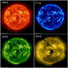 |
Fig. 1. Example images in EIT's four narrow UV bands, taken between 00:00 and 01:19 UTC on January 1, 2003. The intensity in each of these images is scaled logarithmically. The 304 Å band (upper left) observes the chromosphere and transition region, including HeII emission. The 171 Å (upper right), 195 Å (lower left), and 284 Å (lower right) bands observe progressively higher and hotter layers of the transition region and corona, designed to capture Fe IX–X, Fe XII, and Fe XV emission, respectively (Delaboudinière et al. 1995). In quiet periods, the 284 Å band is also contaminated by cooler material, because it overlaps with lines of Mg VII (see, e.g., Young 2023). |
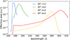 |
Fig. 2. Throughput of the four narrow EIT image bandpasses (Dere et al. 2000). The 171 Å bandpass has the highest peak throughput and the 284 Å bandpass has the lowest. |
In Section 2 we explain the steps we took to reduce each EIT image into a single Sun-as-a-star light curve data point with a motivated uncertainty, accounting both for statistical uncertainty and mission-long instrumental systematics. In Section 3 we present the final EIT light curves, which are available for download from Zenodo1, and compare the EIT light curves to other long-baseline solar photometry from SOHO and from NASA's Solar Radiation and Climate Experiment Extreme-ultraviolet Photometer System (SORCE/XPS; Woods & Rottman 2005), an independent space mission on a different orbit from SOHO operating between 2003 and 2020. We present our conclusions in Section 4, along with a discussion of the utility of these light curves for stellar and exoplanet astronomy.
2. Data reduction
2.1. SOHO's orbit and mission history
SOHO is on an elliptical halo orbit around the first Lagrange point in the Earth-Sun system, with a period of 178 days, or almost exactly 6 months (Vandenbussche & Temporelli 1996). Since launch in 1995, both the SOHO spacecraft and the EIT (see below) have experienced both slow degradation and acute hardware failures of varying severity. We must understand their effect on the EIT data, compensate for them where possible, and account for them in our uncertainty estimation. In Table 1, we enumerate the various causes of missing or bad EIT data addressed in this section.
Reasons for missing or unusable EIT images.
We begin with acute hardware failures. Relevant to our analysis are two major events in SOHO's history: the near-total mission loss between June and October 1998 (see Vandenbussche 1999 for a full historical account) and the high-gain antenna pointing mechanism failure in 2003 (ESA 2003).
The near-mission loss occurred on June 25, 1998, when a pair of interacting software errors caused the spacecraft to lose attitude control and subsequently (because the antennae and solar panels were now pointing the wrong way) telemetry and power. Over four months of careful and creative effort, including using the Arecibo radio telescope and the NASA Deep Space Network 70-meter antenna to find the spacecraft, the SOHO team managed to re-establish contact, re-point toward the Sun, and eventually restore all twelve science instruments to full function. As a result of this event, there were no EIT images taken between June 24 and 12 October 1998, inclusive.
The high-gain antenna (HGA) pointing mechanism began to fail in May 2003. By June, the SOHO team decided to stop trying to move the antenna altogether and instead leave it stationary at an angle where, for the majority of SOHO's orbit, it can point toward Earth accurately enough for data transmission. This configuration necessitates that SOHO rotate by 180° every half-orbit (i.e., every ∼3 months) to keep the antenna pointed toward Earth while SOHO remains pointed at the Sun. Even so, twice per orbit, for approximately two weeks at a time (so-called keyhole periods), the high-gain antenna cannot be used, and the low-gain antenna must be used instead. Since data transmission through this antenna is slower, SOHO prioritizes data transmission from its helioseismic instruments (VIRGO; Global Oscillations at Low Frequencies, or GOLF, and MDI), which depend strongly on uninterrupted time series to achieve their scientific aims, during keyholes. For several years, this meant that no EIT images were taken during these periods.
On August 14, 2009, the HGA position was improved such that EIT operations would no longer be significantly interrupted by keyholes (J.B. Gurman and Jean-Philippe Olive, private comm.), although they remain interrupted every 3−6 months by scheduled instrumental maintenance periods known as CCD “bakeouts”. Starting from 2003, bakeouts were scheduled to deliberately fall during keyhole periods, and they have continued to be scheduled at roughly the same pace even now that keyholes are no longer a problem (see Section 2.6.2). The keyhole-bakeout duty cycle is ≲28 days per ∼178-day orbit (or ≲15%). The periodicity of the keyhole-bakeout events also has a strong effect on the periodogram of the final EIT light curves (see Section 3).
2.2. EIT images
To begin, we downloaded the full catalog of EIT images (∼2 terabytes) from ESA's SOHO science archive2. This catalog includes calibrated images (data processing level L1) from shortly after SOHO's launch in December 1995 to April 1, 2024, inclusive. We present example images in EIT's four EUV passbands in Figure 1. For querying and viewing EIT images from specific dates, or movies constructed from series of EIT images across a range of dates, we refer to the SOHO movie theater3 and JHelioviewer application (Müller et al. 2017). These L1 calibrated EIT images used in this study have been pre-processed with the IDL routine EITprep.pro, available as part of the SolarSoftWare package (Freeland & Handy 1998). This routine consists of the following steps:
-
Subtract the analog-to-digital converter offset, which is measured by taking zero-exposure-time dark frames periodically throughout the mission.
-
“De-grid” the image, to approximately remove the shadows cast on the CCD by the fine wire mesh grids supporting the aperture filter and the filter wheel.
-
Flat-field the image.
-
Normalize the counts per second of exposure time to calculate a flux, in units of data numbers per second.
-
Normalize the flux to the open position in EIT's filter wheel (see Section 2.5).
-
Normalize the flux to account for EIT's declining pixel response over SOHO's lifetime, using a correlation with the Mg II solar activity index (Heath & Schlesinger 1986).
These steps address many, but not all, of the instrumental systematics affecting the EIT data. For example, the flat-field correction accounts for the in-flight degradation of the CCD. It is based on ratios of images of an on-board white light calibration lamp, which are converted to EUV flat-field maps using an empirical relationship. The method satisfactorily corrects the relative spatial response variations, but there are known residuals in the absolute values that create temporal trends in the integrated fluxes. We address the systematics correction, including temporal trends, in Section 2.6.
We restricted our analysis to only images taken after SOHO's commissioning phase was officially complete, on April 16, 1996. We discarded any image that was not taken at EIT's full resolution, 1024×1024 pixels (∼3% of the total). To transmit images back to Earth, the SOHO Large Angle and Spectrometric Coronagraph experiment (LASCO) electronics box, which is shared between EIT and LASCO, divides each image into 32×32-pixel “data blocks” and downlinks the data block by block; we also discarded any image with missing or corrupted blocks (∼9% of the total).
The unit of flux in each EIT image pixel is counts per second; in other words, the images and the resulting light curves tally relative fluxes rather than absolute fluxes in physical units. This is the same as, for instance, Kepler light curves, but different from, for instance, the VIRGO total solar intensity time series, which are in physical units of watts per square meter.
Figure 2, plotted from Tables 6–9 of Dere et al. (2000), shows the throughput of each of EIT's four narrow bandpasses. The bandpasses are defined by multilayer coatings on the four quadrants of the primary and secondary mirrors, but the overall throughput of the instrument (in any of the bandpasses) also depends on the position of the telescope's filter wheel, located between the secondary mirror and the detector. The throughput plotted in Figure 2 corresponds to the filter wheel being set to its open position, with no additional filter (see Section 2.5). We note that the peak throughput differs by more than an order of magnitude between the 171 Å and 284 Å bandpasses; the corresponding (unnormalized) light curves will exhibit the same difference.
A histogram of the cadence of EIT observations in each bandpass is plotted in Figure 4. In all four bands, the modal cadence of the observations is 0.25 days for approximately the first half of the mission, from April 16, 1996, to July 20, 2010. After this, the modal cadence decreases to 0.5 days. Other multiples of 6 hours are also common throughout the mission. The 195 Å bandpass has an additional peak at extremely short cadences (∼10 minutes) because of a short-cadence observational campaign in this bandpass between December 21 and 28, 1996.
2.3. Benchmark solar time series for comparison
We also downloaded several time series from other solar instruments to compare to our EIT light curves and used them to double-check our systematics corrections. The first of these was the VIRGO total solar irradiance time series, re-calibrated by Finsterle et al. (2021), which runs from February 1996 to December 20234. We used the TSI VIRGO/PMO6V-A+B time series (column name TSI_virgo_fused_new), which is a composite time series produced by combining the data from VIRGO's two identical PMO6-V radiometers (PMO6-VA is used continuously, while PMO6-VB is a backup radiometer used to monitor PMO6-VA's degradation over time), along with its associated uncertainty (column name TSI_virgo_fused_unc).
For a long-baseline solar time series with ultraviolet spectral information, we downloaded the mission-long NASA SORCE/XPS spectral irradiance time series (Woods & Rottman 2005) from the Laboratory for Atmospheric and Space Physics Interactive Solar Irradiance Datacenter (LISIRD)5. This data set runs from February 25, 2003, to February 25, 2020, with a gap in observations from August 2013 to February 2014 due to battery degradation (Woods et al. 2021). This data has been extensively calibrated against overlapping observations of the solar spectral irradiance by other instruments, so we have assumed it is not affected by any significant instrumental systematics.
Lastly, we download the version 4 CELIAS/SEM mission-long daily average time series (Hovestadt et al. 1995), which we also obtain from the LISIRD database6. CELIAS/SEM has two bandpasses; the 0th-order channel is a broadband soft X-ray to EUV bandpass, ranging from 1−500 Å. The first-order channel is a narrow bandpass whose response function peaks at an almost identical wavelength to EIT's 304 Å -band response function, as shown in Figure 3. Because of this similarity, we hypothesize that the normalized EIT 304 Å light curve should be essentially identical to the normalized CELIAS/SEM first-order light curve, as long as the respective instrumental systematics have been appropriately corrected.
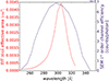 |
Fig. 3. Comparison of the throughput of the EIT 304 Å bandpass (Dere et al. 2000) and the CELIAS/SEM first-order channel bandpass, digitized from Hovestadt et al. (1995) Figure 23. Note: the y-axis in Figure 2 is logarithmic, while the y-axis here is linear. |
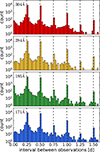 |
Fig. 4. Histograms of the intervals between successive EIT images taken in each of the four bandpasses. The modal cadence in all four filters is 0.25 days, but other multiples of 6 hours are also common. |
We have assumed that the CELIAS/SEM instrumental systematics have been appropriately corrected over short timescales. However, the Laboratory for Atmospheric and Space Physics (LASP) SOHO/SEM Version 4 Science Product release notes (Woodraska 2008) state there is a known issue related to SEM data exemplified by an “uncorrected long-term degradation”, identified by comparing the CELIAS/SEM observations to ALMA observations. We can observe this degradation ourselves in Figure 5 (upper panel), where we plot the ratio of the CELIAS/SEM first-order light curve to a simulated light curve generated by propagating the SORCE/XPS spectral irradiance through the CELIAS/SEM first-order bandpass. This ratio exhibits a linear decline over the SORCE/XPS baseline (2003–2020).
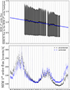 |
Fig. 5. Top panel: Ratio of the CELIAS/SEM first-order light curve to a simulated light curve constructed by propagating the SORCE/XPS solar spectral irradiance through the CELIAS/SEM first-order bandpass. We assume that since SORCE/XPS is well-calibrated against independent measurements of the solar spectral irradiance by other instruments that the decline in this plot is evidence of long-term degradation in the CELIAS-SEM light curve. We fit a line (blue) with linear least squares fitting to account for it. Bottom panel: Uncorrected (black) and corrected (blue) versions of the CELIAS-SEM first-order light curve. |
We fit the ratio with a line, using linear least squares fitting to find the optimal parameters, and then extrapolated the linear fit to cover the entire CELIAS/SEM baseline (1996–2024). We divided the extrapolated line out of the CELIAS/SEM first-order light curve to produce a corrected version (Figure 5, lower panel). We propagated the analytic uncertainties on the line parameters from the least squares fit analytically through to the corrected light curve.
We made extensive use of the corrected CELIAS/SEM first-order light curve in our EIT systematics corrections (see Section 2.6). Before using it, we also performed a simple outlier rejection: we computed a running median of kernel size 11 for the light curve, then discarded any point that is <0.75 or >1.25 times the value of the running median.
2.4. Reducing each EIT image to a light curve data point
To convert an EIT image into a single light curve flux value with an uncertainty, we must account for (i) the flux coming from the solar disk and (ii) the coronal flux coming from beyond the solar limb. As Figure 1 shows, the off-disk contribution is relatively minor in the 304 Å band, which observes the chromosphere and transition region, but increasingly important for the 171 Å, 195 Å, and 284 Å bands, which observes higher layers of the corona. We note that the intensity in each image in Figure 1 scales logarithmically.
The on-disk flux is easy to sum up, because the solar disk is fully contained within the bounds of every EIT image. The off-disk flux requires slightly more care, because the solar disk subtends a different angular diameter in each image depending on SOHO's distance from the Sun. When SOHO is closer to the Sun, the Sun occupies a larger fraction of EIT's field of view and vice versa.
We correct for this effect by normalizing EIT's field of view to that of the EIT image taken at minimum distance from the Sun across the whole EIT baseline (i.e., the image where the solar disk occupies the greatest fraction of the field of view). We calculated the sky-projected physical distance spanned by that image, then we effectively “trimmed” the outermost row(s) of pixels off every other image to create a square of the same physical size. EIT's angular field of view is
 (1)
(1)
where 2.627 arcseconds per pixel is the pixel scale, which is the same for every EIT image in both the x and y-directions (Auchère et al. 2000).
When SOHO is at its minimum distance from the Sun, Dmin, the sky-projected physical distance spanned by the image is
 (2)
(2)
The angle that subtends the same physical distance, p, when SOHO is at an arbitrary distance, D, from the Sun is
 (3)
(3)
and the corresponding diameter of the image, in units of pixels, is
 (4)
(4)
where δ is expressed in arcseconds. The diameter of the image in pixels, dpix, varies from 988 pixels at SOHO's maximum heliocentric distance to 1024 pixels at SOHO's closest approach.
We proceeded by summing up the flux in each image, out to its normalized diameter, dpix. Figure 6 shows our approach to tallying the on- and off-disk flux in each image graphically. Briefly, to include as much off-disk flux as possible, we extrapolate beyond the bounds of the image to include an estimate of all the flux within a circle of radius  pixels of the center of the Sun, where rpix=dpix/2. In other words, rpix is the distance between the center of the Sun and any corner of the image, assuming the Sun were perfectly centered.
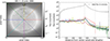 |
Fig. 6. Left panel: Example EIT 195 Å image taken on June 15, 1996. The curved arrow shows the direction of the solar rotation. The eight bisecting lines meet at the center of the solar disk, (icenter,jcenter). The image is color-mapped by the logarithmic flux value in each pixel in units of counts per second. The black square just inside the border of the image is the “trimmed” square of side length 2rpix centered at the center of the solar disk. Right panel: Flux value per pixel along each example bisecting line as a function of distance from (icenter,jcenter). Note that, beyond the solar limb at r≃363 (the leftmost vertical dashed line indicates the photospheric radius), the lines that intersect the solar poles (yellow and magenta) have much lower average flux per pixel than the other lines, due to significantly fainter coronal emission from a polar coronal hole. The black line with (barely visible) error bars is the total flux in each annulus from radius r = 1 to |
To carry out this extrapolation, we divided the image into narrow annuli centered at the center of the solar disk, and sum up the flux contribution from each annulus. Annuli with outer radii larger than rpix pixels overlap with the edge of the image, so for these annuli, we linearly extrapolated the flux from the observed segment of the annulus to calculate the flux expected from the full annulus.
For each EIT image, we began by calculating the x and y indices of the pixel closest to the center of the solar disk, using metadata from the FITS header. Every EIT image has the same reference pixel, located at the center of the CCD, at position (iref,jref) = (512.5,512.5) pixels (recorded in header keywords CRPIX1 and CRPIX2).
However, the x-axis of the CCD array is not necessarily aligned with the solar equator and the center of the CCD is not necessarily aligned with the center of the Sun. The header keyword CROTA gives the rotation angle, θrot (in degrees) between the CCD x-axis and the solar x-axis (in helio-projective Cartesian coordinates), defined by the solar equator. The header keywords CRVAL1 and CRVAL2 give the helio-projective Cartesian coordinates of the reference pixel of the CCD (in arcseconds).
We proceeded by transforming the position of the reference pixel (CRVAL1 and CRVAL2) to the CCD coordinate system:
![Mathematical equation: $$ {\left [\begin {array}{c} x_{\mathrm {ref}} \\ y_{\mathrm {ref}} \end {array}\right ]} = {\left [\begin {array}{cc} \cos {\theta _{\mathrm {rot}}} &\sin {\theta _{\mathrm {rot}}} \\ -\sin {\theta _{\mathrm {rot}}} &\cos {\theta _{\mathrm {rot}}} \end {array}\right ]} {\left [\begin {array}{c} \mathrm {CRVAL1} \\ \mathrm {CRVAL2} \end {array}\right ]}. $$](/articles/aa/full_html/2025/07/aa54946-25/aa54946-25-eq7.gif) (5)
(5)
By converting the vector (xref,yref) to units of pixels and following it backwards from (iref,jref), we can find the CCD coordinates of the origin of the helio-projective coordinate system, namely, the solar center:
 (6)
(6)
Most EIT images are near-centered on the Sun, with (icenter,jcenter)≃(508,518). In the left panel of Figure 6, the bisecting lines meet at (icenter,jcenter).
We proceeded by dividing the image into annuli of width 1 pixel, centered at (icenter,jcenter), stepping outward in radius from r = 1 pixel to  pixels. Pixels with indices (i,j) where
![Mathematical equation: $$ \left (r - \frac {1}{2}\right )^2 < [(i - i_{\mathrm {center}})^2 + (j - j_{\mathrm {center}})^2] \leq \left (r + \frac {1}{2}\right )^2 $$](/articles/aa/full_html/2025/07/aa54946-25/aa54946-25-eq10.gif) (7)
(7)
belong to the annulus of radius, r. For r≲512, the entire annulus is contained within the boundaries of the square image, so the total flux in the annulus is
 (8)
(8)
where the sum is over all N pixels in the annulus of radius, r. We approximate the uncertainty on the total flux in the annulus as Poisson uncertainty, given by
 (9)
(9)
We note that this estimate formally underestimates the appropriate uncertainty on Fr, because it does not include for thermal signal in the CCD; however, given that the CCD is operated at a temperature of ∼−70°C, we expect the thermal signal to be negligible compared to the solar signal.
For r≳512, the annulus overlaps the edge of the image, and we must extrapolate beyond the known pixels to estimate the total flux in the annulus. We did this by calculating the total flux value over the Nknown observed pixels in the annulus,
 (10)
(10)
and then linearly scaling this known flux to the extrapolated number of pixels that would be in the annulus if the image were bigger, Nextrapolated = 2πr. The total flux in the annulus is then
 (11)
(11)
and its uncertainty, propagated analytically, assuming uncorrelated noise, is
assuming that  . The right panel of Figure 6 shows the flux in each annulus as a function of its radius r and its uncertainty. The uncertainties for the annuli overlapping the edge of the image are (appropriately) very large.
We obtain the total flux in the image, Fimage, and its associated uncertainty by summing the annular fluxes in quadrature:
where rmax is the maximum distance, in units of pixels, between (icenter,jcenter) and any corner of the image. The flux in each image is generally dominated by the on-disk flux. For the 284 Å band, where the off-disk region is brightest, the off-disk flux contributes ∼25−30% of the total. The off-disk flux in the extrapolated region (r≳512) is contributes at most ∼5% to the total.
2.5. Identifying and discarding bad light curve points
After using the above procedure to create preliminary light curves in each of the four EIT bands, we identified and discarded the individual light curve data points afflicted by instrumental problems. The first problem is that EIT's front aluminium heat-rejection filter (see Section 2.1 of Delaboudinière et al. 1995) developed small pinholes early in the mission, likely during launch. These pinholes allow excess light through to the optical cavity and cause bright spots to appear along the edges of some of the EIT images; see Figure 7 for an example. Due to the position of the pinholes, the 284 Å band is much more frequently affected than any other band.
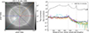 |
Fig. 7. Same as Figure 6 but showing an example EIT 284 Å image taken on July 31, 1996, with bright spots along its upper edge caused by pinholes in EIT's front filter. We note the significant bump in annular flux at r≃500 due to the pinholes. The three patches we use to identify images with pinholes are shown with white outlines; only the two larger patches are necessary for this particular image, but the smaller patch is useful for catching images in the 304 Å filter with smaller pinholes. |
Luckily, EIT was built with a redundant aluminium filter along its optical path. In the early years of the SOHO mission, this filter was not used, in order to keep exposure times as low as possible. However, during this time, the front filter began to peel away from its mounting, leading to a dramatic increase in leaked light onto the CCD, so in May 1998, the operations team decided to start using the redundant filter in order to block this light. The EITprep.pro routine (see Section 2.2) normalizes the flux in each EIT image to the value it would have without this additional filter (i.e., normalizes it to the open position in the filter wheel), so images before and after May 1998 are still directly comparable.
Because the pinholes always appear in the same part of the image, it is easy to identify images that display them. We define three patches enclosing the worst pinhole spots, each of which is a circle cut off at the top by the edge of the image: one at (i,j) = (557,1016) of radius 40 pixels, one at (i,j) = (130,1022) of radius 150 pixels, and one at (i,j) = (585,1022) of radius 200 pixels. These latter two are also cut off below j = 931 to avoid catching too much of the corona, which is actually (and not spuriously) bright. The three patches are plotted as white outlines in Figure 7.
For each pre-May 1998 image, we calculate the mean flux per pixel within each patch and compare it to the mean flux per pixel in a reference patch of the same size, shape, and i-index, reflected across the solar equator. If the mean flux per pixel in any of the three pinhole patches is more than twice the mean flux per pixel in its respective reference patch, we flag the image as containing a pinhole and discard it. We discarded 17 out of 22645 304 Å images (0.08%), 1276 out of 22673 284 Å images (5.6%), 9 out of 23354 195 Å images (0.04%), and 6 out of 22574 171 Å images (0.03%) because of pinholes. The 284 Å light curve, the worst affected, has no data between August 1996 and May 1998.
The second cause of bad data points is solar proton events (SPEs), outbursts of energetic protons associated with high-energy solar flares or coronal mass ejections. Solar proton events cause a static-like pattern across EIT's CCD and result in the CCD recording artificially low flux values. This static appears in images taken in all four EIT bands during the SPE.
To identify and discard SPE-affected images, we download the NOAA Space Environment Services Center catalog of SPE events7. We consider the 141 SPEs in this catalog that occurred between the beginning of SOHO's post-commissioning operations on April 16, 1996, and the end of our current data set on April 12, 2024.
For each SPE, we calculated the “rise time”, trise, as the interval between its beginning and time of maximum tmax, both given in the catalog. We then discarded any EIT image taken within the interval [tmax−2trise,tmax+4trise], which by inspection is sufficient to bracket the entire associated dip in EIT flux for all 141 SPEs. In total, we discarded 1045 images from the 304 Å band, 1049 images from the 284 Å band, 1046 images from the 195 Å band, and 1052 images from the 171 Å band due to SPEs.
After converting the images into preliminary light curves, we also eliminated and discarded a handful of outlying data points which are either anomalously low or anomalously high in flux. We identified these points by the same procedure as the CELIAS/SEM light curve outlier rejection: computing a running median of kernel size 11 for each light curve, then discarding any point that is <0.75 or >1.25 times the value of the running median. An inspection of the images corresponding to these outliers suggests that they are due to one-off camera errors (i.e., most of these images appear blurry, underexposed, overexposed, or some combination). We discarded 19 outliers from the 304 Å light curve, 19 from the 284 Å light curve, 28 from the 195 Å light curve, and 14 from the 171 Å light curve.
2.6. Light curve-level systematics corrections
Before the preliminary EIT light curves can be treated as Sun-as-a-star observations, we must make several systematics corrections at the light curve level.
2.6.1. Heliocentric distance correction
First, SOHO's heliocentric distance varies significantly throughout its orbit. This has two effects: first, that the Sun appears correspondingly larger or smaller in EIT's field of view, and second, that the observed solar flux varies according to the inverse square law. We corrected for the first effect by trimming each image to match the physical dimensions of the image taken at SOHO's closest approach to the Sun. To correct for the second, we normalize each light curve data point by SOHO's heliocentric distance, d, at the time of its observation, to a reference heliocentric distance of 1 AU:
 (12)
(12)
2.6.2. Correcting for 304 Å exponential degradation and CCD bakeouts
Next, we have to account for systematic changes to EIT's sensitivity, beyond those already divided out by EITprep.pro. We can identify these by examining the mission-long time series of the ratio of the normalized EIT 304 Å light curve to the normalized CELIAS/SEM first-order light curve, plotted in the upper panel of Figure 8.
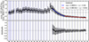 |
Fig. 8. Upper panel: Ratio of the normalized EIT 304 Å light curve to the CELIAS/SEM first-order light curve. The two exponential functions fit to the post-2012 dropoff are plotted in blue and red, respectively, with best-fit parameters given in the figure legend. t1, the beginning of the first exponential trend, is January 11, 2012, and t2, the beginning of the second exponential trend, is June 3, 2016. Note that the SEM time series ends on February 8, 2024 (earlier than our EIT light curves), so this ratio plot also ends on 8 February 2024. Lower panel: Residuals of the exponential fit. |
The vertical blue lines in this figure mark “bakeout” periods. EIT's optical cavity is not a perfect vacuum; there is a small amount of volatile material inside, probably water and hydrocarbons (Moses et al. 1997; Gurman 2007). This material tends to condense onto the CCD, which is kept cold by passive radiative cooling through the shadowed side of the telescope, and block some EUV light. The EIT operations team periodically heats up (or bakes out) the CCD to evaporate this material. Additionally, the bakeouts help maintain the CCD's performance by fixing “electron traps”, which are wells of trapped charge in random pixels caused by cosmic ray hits and EUV overexposure (Gurman 2007).
As Figure 8 shows, there are local trends in the EIT 304 Å to CELIAS/SEM ratio specific to each inter-bakeout period and also an approximately exponential decrease in this ratio from early 2012 onward. Curiously, while the local inter-bakeout trends affect all four EIT bands in a similar way, the late exponential dropoff appears to only affect the 304 Å band. The evidence for this being 304 Å -specific behavior includes (i) that there is no exponential trend in the ratio of any of the other three bands to any independent instrument and (ii) that the flux values in all four EIT bands have a first-order linear relationship to each other before 2012, but this relationship breaks down between the 304 Å band and any other band from 2012 onward. Meanwhile, the linear relationships between the 284 Å, 195 Å, and 171 Å bands persist throughout the mission (see Figure 10).
We hypothesize that this is due to the 304 Å band's known high sensitivity to both molecular condensation onto the CCD and to radiation-induced degradation, which are the two problems that CCD bakeouts attempt to ameliorate, compared to the other bands. As can be seen from the vertical blue lines in Figure 8, the 304 Å exponential trend begins relatively shortly after the decision to decrease the frequency of bakeouts, first to every six months (starting in mid-2010) and then to every year (starting in mid-2016). It is possible that these less frequent bakeouts are failing to fully compensate for the effects of condensation or electron traps on the 304 Å images.
To proceed, therefore, we fit two exponential functions to the ratio of the EIT 304 Å light curve to the CELIAS/SEM light curve, using simple linear least-squares fitting, taking the form
 (13)
(13)
where R is the ratio of the two light curves. The first exponential function is to the time interval between t1 = January 11, 2012, or JD 2455938.417 (the end of the bakeout corresponding to the visible onset of the exponential trend) and June 3, 2016 (the end of the bakeout corresponding to the change from baking out every six months to every year), so tref=t1. The second is to the time interval between tref=t2 = June 3, 2016, or JD 2457542.583333, and the end of the time series. The best-fit exponential functions are plotted in blue and red, respectively, in the upper subplot of Figure 8, and the residuals left over in the ratio after these exponential trends are divided out are shown in the lower subplot of Figure 8. The best-fit parameters and their uncertainties are given in Table 2.
Best-fit parameters of the two exponential functions fit to the ratio of the normalized EIT 304 Å light curve to the CELIAS/SEM first-order light curve with linear least-squares fitting.
We propagate the uncertainties in the parameters of the best-fit exponential functions through to the uncertainties on the corrected EIT 304 Å light curve data points analytically,
![Mathematical equation: $$ F_{\mathrm {exp.\,corrected}} ={} \frac {F}{\exp {[A(t-t_{\mathrm {ref}}) + B]}}, $$](/articles/aa/full_html/2025/07/aa54946-25/aa54946-25-eq20.gif) (14)
(14)
where A, B, σA, and σB are given for both exponential fits in Table 2.
After correcting for the exponential trend, we must next correct for the inter-bakeout trends, which affect all four EIT bands. We make the assumption that each inter-bakeout trend can be modeled by a linear offset to the EIT light curve. There are 84 bakeouts that occur during our light curve baseline, plus one currently unexplained flux discontinuity between December 29 and 30, 2023; these mark the boundaries between each inter-bakeout segment. Using a linear least-squares fitting, we fit a line to each inter-bakeout segment of the EIT 304 Å to CELIAS/SEM light curve ratio. We then divide this line out of all four of the EIT light curves.
We once again propagated the uncertainties on the best-fit line through to the uncertainties on the corrected light curves analytically, as
 (15)
(15)
where F is given by the Fexp. corrected in the case of the 304 Å light curve, and by the uncorrected F for the other three bands, and tref is the start time of each inter-bakeout segment. Because there are 86 segments, we do not enumerate all the best-fit m and b values here. Meanwhile, for each inter-bakeout segment, the corrected flux uncertainty is given by

We note that what is implicit in this procedure is the assumption that there is a linear relationship between all four of the EIT light curves (see below for further discussion). Figure 9 shows the linear fits to each inter-bakeout segment of this ratio and the residuals in this ratio after the linear trends were removed.
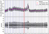 |
Fig. 9. Upper panel: Ratio of the normalized EIT 304 Å light curve to the CELIAS/SEM first-order light curve. The linear functions fit to each inter-bakeout period are plotted in pink. The vertical red line marks November 12, 2008, the (rough) time after which the inter-bakeout trends start to get noticeably worse. Note: SEM time series ends on February 8, 2024 (earlier than our EIT light curves), so this ratio plot also ends on February 8, 2024. Lower panel: Residuals of the linear fits. |
We note here that the inter-bakeout trends only cause the EIT 304 Å to CELIAS/SEM light curve ratio to diverge significantly from 1 from roughly 2008 onward. Therefore, we produced two versions of our final light curves: in version (1), the inter-bakeout trend correction was done for the entire mission lifetime; and in version (2), it was only done from November 12, 2008, onward. Because the inter-bakeout trend correction increases the uncertainty on the corrected light curve data points, version (1) has approximately homoscedastic uncertainties. Version (2) has very different uncertainty characteristics pre- and post-2008, but the uncertainties before 2008 are much smaller. Either version could be more appropriate for various types of Sun-as-a-star analysis, depending on the desired uncertainty properties.
2.6.3. Additional vertical offset correction for 284 Å, 195 Å, and 171 Å bands
This procedure is sufficient to correct the inter-bakeout trends in the EIT 304 Å band light curve, as the residuals in Figure 9 show. However, even after dividing out the linear trends, the other three light curves are still noticeably discontinuous across the post-November 2008 bakeouts, particularly in the period between 2008 and 2012. To address these discontinuities, we adjusted our systematics model to allow a constant vertical offset to each other EIT light curve (284 Å, 195 Å, 171 Å) for each inter-bakeout period.
To find the appropriate vertical offset, we began by reiterating our hypothesis that the 284 Å, 195 Å, and 171 Å light curves have a linear relationship to each other, at least to first order. Figure 10 shows this linear relationship; here, we plot each of the version (2) light curves against each other (i.e., these light curves have had the linear inter-bakeout trends based on the 304 Å to CELIAS/SEM ratio removed, but only from November 12, 2008, onward). For clarity, we chose not plot to the uncertainties of the data points.
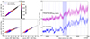 |
Fig. 10. Left: Scatter plots of the light curves in the EIT 171 Å 195 Å and 284 Å bands, after the initial corrections to the post-November 12, 2008, inter-bakeout segments are applied. All data points pre-November 12, 2008, are plotted in black; the later points are color-mapped by observation time. The uncertainties of the points are not plotted, for clarity. Straight lines show projections of the three-dimensional line of best fit to the pre-November 12, 2008, data. Blue plus symbols show the inter-bakeout segment between July 22, 2011, and January 6, 2012. Magenta plus symbols are the same inter-bakeout segment with additional constant offsets applied to move it closer to the line of best fit along the shortest possible vector. Right: Segment of the EIT 171 Å light curve, from November 12, 2008, to late 2014, when the bakeout discontinuities are most extreme. In blue is the light curve with only the initial bakeout correction applied; in magenta is the light curve with an additional constant offset added per bakeout. The magenta light curve is offset by +0.65 compared to the blue one for plotting clarity. The discontinuities across the bakeouts are much less extreme in the magenta version. The shaded region shows the inter-bakeout segment between July 22, 2011, and January 6, 2012, highlighted in the left panel. |
The line in each subplot of Figure 10 represents the best straight-line fit to the pre-November 12, 2008, data. We note that all three light curves have been normalized by their median value, to make it easier to set sensible priors on the fit parameters. Because our light curve fluxes are uncertain in all three bands, we specify a model where each two-dimensional projection of this best-fit line has three parameters: a slope, m, an intercept, b, and an intrinsic scatter orthogonal to the line, V. We performed the fit to each two-dimensional projection with the Markov chain Monte Carlo (MCMC) routine emcee in a transformed parameter space θ,b cos θ,V, where θ=arctanm, following the recipe given in Hogg et al. (2010), Sections 7 and 8 (specifically, the likelihood function for the fit is given by their Equation 35). The priors for this fit are given in Table 3 and the parameters of the best-fit line are given in Table 4.
Priors for the MCMC fit of the linear model with scatter to the relationship between the pre-November 12, 2008, EIT 171 Å, 195 Å, and 284 Å normalized light curves.
Parameters of the best-fit line to the relationship between the pre-November 12, 2008, EIT 171 Å, 195 Å, and 284 Å normalized light curves.
We assume that, if the bakeouts are appropriately corrected, that all of the data should lie as close to the best-fit pre-November 12, 2008, line as possible. For a given inter-bakeout segment, we calculate the shortest three-dimensional vector between the point (m171,m195,m284), where m171 is the median value of the 171 Å light curve during segment, and the three-dimensional line of best fit to the pre-November 12, 2008, data, the two-dimensional projections of which are plotted in Figure 10. The three components of this vector are the vertical offsets we apply to each light curve to in order to minimize discontinuities across bakeouts.
The left panel of Figure 10 shows this procedure graphically for the inter-bakeout segment beginning July 22, 2011, and ending January 6, 2012. The blue symbols show the light curve data from this segment before the vertical offsets are calculated and applied; the magenta symbols show the data after the correction. The right panel of Figure 10 shows the EIT 171 Å light curve during early Solar cycle 24, when the bakeout discontinuities are most extreme, before and after the vertical offsets are applied. Applying the offsets significantly ameliorates the discontinuities.
For the version (1) light curves, we repeat this vertical offset correction procedure for every inter-bakeout segment where it is possible. It is not possible for the inter-bakeout segments in 1996 and 1997, where there is no 284 Å data due to the filter pinhole problem because the three-dimensional point (m171,m195,m284) is not defined for these segments. For the version (2) light curves, we repeat the vertical offset correction procedure for only the inter-bakeout segments after November 12, 2008.
2.6.4. Viewing angle correction
Lastly, we introduced another small correction to the bakeout-corrected light curves, to account for SOHO's variable viewing angle on the Sun throughout its orbit. Because of the tilt of the ecliptic plane with respect to the solar equator, and the tilt of SOHO's orbit with respect to the ecliptic plane, SOHO's heliocentric latitude varies between approximately −7.5° and +7.5°. Naively, we would expect that, because the solar corona is brighter at the Sun's active latitudes than at the poles, the EIT light curve points taken at higher latitudes, where more of the pole is visible, should be fainter.
Figure 11 shows the four EIT light curves, sorted by heliocentric inertial latitude. In order to prevent the solar activity cycle or the solar rotation from dominating this plot, we divide up the EIT light curves into segments corresponding to one quarter of SOHO's orbit, and normalize each segment by its median flux value. In the first quarter, SOHO sweeps from heliocentric latitude 0° to +7.5°; in the second quarter, from +7.5° back to 0°, and so on.
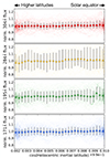 |
Fig. 11. Four EIT version (2) light curves, shown as small points, plotted against the cosine of SOHO's heliocentric inertial latitude. cos(lat) = 1, at the right-hand side of the plot, corresponds to a SOHO heliocentric latitude of 0°, or a viewing angle directly onto the equator. To prevent this plot from being dominated by the solar activity or rotation cycles, we divide each light curve into segments according to SOHO's heliocentric latitude and normalize the flux per segment (see text for details). |
To establish whether there is a trend in the data with heliocentric latitude, we fit the light curves as plotted in Figure 11 with three competing models and evaluate the Bayesian evidence for each. The first model has no dependence on heliocentric latitude,
 (16)
(16)
The second is linear in the absolute value of heliocentric latitude, l,
 (17)
(17)
The third is linear with respect to the cosine of heliocentric latitude,
 (18)
(18)
where l0 is the minimum heliocentric latitude across the time series.
We used the dynamic nested sampler from the python package dynesty (Speagle 2020) to perform the fits and the evidence calculation. The priors for these fits are given in Table 5 (although the outcome of the model selection is not sensitive to the choice of boundaries on these priors). We repeated this procedure for both version (1) and version (2) of the light curves.
Priors for the nested sampling fit of each normalized light curve as a function of heliocentric latitude.
The natural logarithm of the Bayesian evidence ratios for the various models are presented in Table 6. In almost every case, the model that is linear in the cosine of heliocentric latitude is decisively preferred over the other two. The exception is the version (2) 304 Å light curve, for which the model that is linear in heliocentric latitude is preferred. In every case, the Bayes factor, equal to Zlinear cos/Zlinear, has a magnitude greater than 10, meaning that the preference is strong.
Comparison of the Bayesian evidence for the three models: the constant model is independent of heliocentric latitude; the linear model is linear in heliocentric latitude; and the linear cos model is linear in the cosine of heliocentric latitude.
Finally, we divided out the preferred model from each light curve, again propagating the uncertainties in the best-fit model parameters analytically to the corrected light curve data points. For all but the version (2) 304 Å light curves, the corrected flux is then given by
 (19)
(19)
For the version (2) 304 Å light curves, it is given by
 (20)
(20)
The corrected uncertainty, finally, is given by
where m,b=ml,bl for the version (2) 304 Å cases and mc,bc for all other cases.
3. Results
In this section, we present our final EIT light curves in all four bands, which we produced by applying the data reduction procedures and systematics corrections described in Section 2. We publish two versions of each Sun-as-a-star light curve: version (1) uniformly corrected for instrumental systematics across the whole mission lifetime (except the inter-bakeout segments in 1996 and 1997 with no 284 Å data, where vertical inter-bakeout segment offsets cannot be calculated, as noted above) and version (2) corrected for bakeout systematics only after November 12, 2008. For completeness, we also publish versions (1) and (2) without the final correction for viewing angle outlined in Section 2.6.4. Table 7 summarizes the differences between the various versions and suggests use cases for each.
Description of the four published final versions of each EIT light curve.
Figure 12 shows the final version (2), viewing angle-corrected light curves in all four EIT bands. The upper panel shows the un-normalized light curves in their original units of [count/s], so the different efficiencies of the four EIT bandpasses are clearly visible (see Figure 2). The 171 Å bandpass has the highest transmission, and the 284 Å light curve has the lowest. The lower panel shows the same light curves normalized by their respective median values.
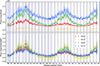 |
Fig. 12. Final EIT light curves, corrected for instrumental systematics and for EIT's viewing angle. These are the version (2) light curves, for which the linear bakeout trend correction is only performed after November 12, 2008; as a result, the light curve uncertainties after this date are much larger than before this date. Upper panel: Un-normalized light curves in their original units. Lower panel: Same light curves, each normalized by its median value. |
The overall modulation due to solar cycles 23 (mid-1996 to late 2008), 24 (late 2008 to late 2019), and 25 (late 2019 onward) is clearly visible in all four light curves, with the maximum in cycle 23 being stronger than the maximum in cycle 24, as expected from other solar observations. Over the solar cycle, the 284 Å band light curve has the highest peak-to-peak fractional variability (320%), followed by the 195 Å band (230%), the 304 Å band (160%), and finally the 171 Å band (130%). The solar rotation cycle is also visible in all four light curves, with the strongest fractional variability again apparent in the 284 Å band, which traces active regions most directly.
It is clear from Figure 12 that residual bakeout discontinuities persist in the version (2) light curves; for example, the bakeout ending September 1, 2001, coincides with a discontinuity in all four light curves. This discontinuity is significantly ameliorated in the version (1) light curves due to their larger uncertainties in the first half of the mission lifetime.
Figure 12 also suggests, tentatively, that there may be an uncorrected systematic decline in the 304 Å light curve from at least 2008 onward. This decline can be seen by comparing the normalized 304 Å light curve to the normalized 171 Å light curve. Over solar cycle 23, the 304 Å flux is generally greater than the 171 Å flux, but the two light curves level out to be roughly the same at solar minimum in 2008−2009, and after ∼2011, the 304 Å flux is generally lower than the 171 Å flux.
Because we calibrate the EIT 304 Å light curve under the assumption that the degradation-corrected CELIAS/SEM first-order light curve represents the ground truth, this yet-uncorrected degradation may indicate that our linear degradation correction (see Figure 5) is not sufficient over the latter half of the mission. We therefore encourage caution when using our 304 Å EIT light curve, particularly over long baselines.
Figure 13 shows Lomb-Scargle periodograms (Lomb 1976; Scargle 1982), computed with astropy.timeseries.LombScargle, of the four EIT light curves and of the window function imposed by EIT's observation schedule (i.e., a constant time series with the same “observation times” as the EIT light curve). The window function has excess power at frequencies corresponding to 1 year (Earth's orbital period, and therefore L1's orbital period) and harmonics of SOHO's orbital period around L1 (PSOHO∼178 days). The EIT light curves also have excess power at these frequencies, particularly PSOHO/2 and PSOHO/4, which makes sense given the symmetry of the orbit and the twice-per-orbit keyhole periods. The EIT light curves also have excess power at and around the solar rotation period of ∼27 days.
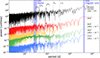 |
Fig. 13. Lomb-Scargle periodograms of the version (2) light curves presented in Figure 12, as well as of the window function of the observations. A multiplicative offset has been applied to each periodogram to render them all visible on the same plot. The window function has significant power at frequencies corresponding to 1/2 and 1/4 of SOHO's orbital period, because EIT does not take data during SOHO's keyhole periods, which occur twice per orbit. There is also excess power in the window function at 1/6 of SOHO's orbital period. All four light curves have excess power at the solar rotation period, while the window function does not. |
We next evaluate whether the solar rotation period could be recovered from our light curves under observational constraints similar to those of a short-baseline photometric monitoring campaign, such as an exoplanet transit survey. We split each of our light curves up into one-year segments by calendar year of observation, yielding 29 segments per light curve. We note that the first and last segments are shorter than one year, as the 1996 segment only includes data from April to December, and the 2024 segment only includes data from January to April. Next, following the method of Angus et al. (2018) for inferring probabilistic stellar rotation periods from light curve data and using the python package celerite (Foreman-Mackey et al. 2017), we fit each segment using a Gaussian process model with a quasi-periodic covariance kernel, the form of which is given by Foreman-Mackey et al. (2017) via Equation (56):
![Mathematical equation: $$ \kappa (\tau ) = \frac {B}{2+C}e^{-\tau /L}\left [\cos {\frac {2\pi \tau }{P_{\mathrm {rot}}}} + (1+C)\right ]. $$](/articles/aa/full_html/2025/07/aa54946-25/aa54946-25-eq30.gif) (21)
(21)
Here, Prot is the rotation period; the other parameters have less direct physical interpretation, but (depending on their numerical values) the covariance function describes a time series where points separated by nProt are correlated, with the strength of the correlation decaying for increasing n.
For each year-long EIT light curve segment, we fit the parameters of this covariance function using emcee (Foreman-Mackey et al. 2013). The priors of the emcee fit are given in Table 8. We considered a fit to be “converged” if the maximum a posteriori solution is not within 1 day of either the lower or upper limit of the lnProt prior.
Priors for the MCMC fit of the Gaussian process model to each light curve segment.
We repeated this experiment for the VIRGO total solar irradiance time series as well. The results for EIT and VIRGO are plotted in Figure 14. We only show the data points for which the Gaussian process model fit converged: 18 of the 29 segments for the 304 Å light curve, 27 of the 28 segments for 284 Å (recall that there is no usable data in the 284 Å band in 1997 due to pinholes), 23 of the 29 segments for 195 Å, and 19 of the 29 segments for 171 Å, and 10 of the 29 segments for VIRGO. The shaded horizontal band in Figure 14 shows the range of the true solar rotation period, from equator to pole, calculated analytically from the solar differential rotation equation given by Snodgrass & Ulrich (1990). The near-horizontal black curves represent the average rotation period behavior of sunspot groups over the solar activity cycle, as calculated by Jiang et al. (2011).
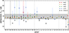 |
Fig. 14. Recovered rotation periods from a Gaussian process fit to segments of each EIT version (2) light curve and the VIRGO light curve, split up by calendar year of observation. Each band has a small x-offset for plotting clarity. The gray shaded band shows the range of the true solar rotation period, from equator to pole, calculated analytically from the solar differential rotation equation given by Snodgrass & Ulrich (1990). The near-horizontal black curves represent the average behavior of migrating sunspot groups over the solar activity cycle, as calculated by Jiang et al. (2011). The true solar rotation period can be recovered from the 284 Å light curve in 26 out of 29 years, and from the VIRGO light curve in only 3 out of 29 years. |
For the 284 Å light curve, the maximum a posteriori rotation period value is 1σ consistent with the true solar rotation for 26 out of 28 segments. The only years for which the true solar rotation period is not recoverable from the 284 Å light curve are 2006, when the maximum a posteriori rotation period slightly underestimates the true value, and 2018, when the maximum a posteriori rotation period abuts the upper limit of the rotation period prior. The uncertainty on the best-fit period in 2024 is extremely large, because the 2024 baseline is only ∼3 months.
Meanwhile, the true solar rotation is recovered for 23 of the 29 segments of the 195 Å light curve, 18 of the 29 segments of the 171 Å light curve, 18 of the 29 segments of the 304 Å light curve, and only 3 of the 29 segments of the VIRGO light curve. In most cases where the VIRGO fits converge, they underestimate the true solar rotation period. There is nothing obviously wrong with the fits that converge to a low value, and changing the bounds on the parameter priors does not significantly affect the results.
The difference between the success of this exercise in the EUV versus the optical is stark: for the 284 Å band, which directly traces coronal activity, the solar rotation period is recoverable 93% of the time, including in 1996, where there are only ∼8.5 months of light curve data. Meanwhile, for the VIRGO TSI time series, which is dominated by optical light, the solar rotation period is only recoverable 10% of the time. Changing the prior ranges for lnB, lnC, and lnL has no significant effect on this result.
4. Discussion and conclusions
Here, we present Sun-as-a-star light curves from the SOHO EIT images in four narrow EUV bands, tracing solar activity in the chromosphere (at 304 Å) and corona (at 284 Å, 195 Å, and 171 Å) across 28 years and 2.5 solar activity cycles, available for download from Zenodo1. For the first time, it is possible to directly compare EIT's extremely detailed picture of activity on the Sun to observations of other Sun-like stars.
Furthermore, we find that these EUV light curves are better tracers of the solar activity cycle than the Sun's optical light curve. The Sun's fractional variability over the solar cycle is much higher at UV and X-ray wavelengths than at optical wavelengths. Our EIT 284 Å light curve has a peak-to-peak fractional variability of 320% over SOHO's baseline; over the same baseline, the fractional variability in the VIRGO total solar irradiance time series is only 0.3%.
The EIT light curves are also substantially more sensitive to the rotation of solar activity features than optical light curves. To test this, we divided our light curves up into year-long segments and attempted to infer the solar rotation period from each. We find that we can accurately recover the solar rotation period for 26/28 year-long segments of the EIT 284 Å light curve (93%), compared to only 3 of the 29 year-long segments of the VIRGO light curve (10%). This result agrees nicely with recent other work on the detectability of solar rotation at different wavelengths; Vasilyev et al. (2025); for example, we used the SATIRE-S solar spectral irradiance data to calculate the probability of accurately recovering the solar rotation period from light curve data at wavelengths between 2000 Å and 10 000 Å, concluding that at optical wavelengths (≥400 nm), the probability of detecting the true Prot at a random phase in the solar cycle is less than 20%, while at UV wavelengths (<400 nm), the probability is as high as 80%.
These results are aligned with expectations from the literature on stellar activity: a star's UV emission is known to trace its activity state and phase in its magnetic cycle (if it has one). In turn, it is important to know the activity state because it can affect the precision and accuracy of RV measurements of the star (see, e.g., Santos et al. 2010; Lovis et al. 2011; Dumusque et al. 2011; Meunier 2024) and because it determines the strength of the stellar wind (see, e.g., Vidotto et al. 2012). In other words, the activity state, which is directly traced by the UV emission, bears directly on both the detectability and habitability of any planets in the stellar system. The EUV flux itself, and its variability, are also important to understand, as they are likely to have significant effects on the chemistry and thermal structure of the atmospheres of any surrounding planets. We refer to National Research Council (2012) for a detailed interdisciplinary review of the effects of solar variability on Earth's climate.
However, UV observations of stars are much scarcer than optical observations, especially in the current age of high-quality, long-baseline, high-cadence photometric observations of hundreds of thousands of stars taken by exoplanet transit surveys, including Kepler and the Transiting Exoplanet Survey Satellite (TESS). For example, broad-band near-UV photometry (1350−2750 Å) from the Galaxy Evolution Explorer (GALEX; Martin et al. 2005) mission's All-Sky Imaging Survey has been used to study the UV emission of nearby M-dwarfs (Shkolnik et al. 2011; Stelzer et al. 2013) and Sun-like stars (Findeisen et al. 2011) and to compare this UV emission to optical activity indicators from spectra, including Hα emission and  , finding general positive correlation, but large scatter. For their sample of Sun-like stars, Findeisen et al. (2011) concluded that roughly half of this scatter is attributable to observational uncertainty and the other half to long-term, activity-related UV variability across their stellar sample. At shorter wavelengths, EUV and X-ray photometric measurements have also been taken for hundreds of Sun-like stars in order to study the relationship between high-energy emission and stellar age (e.g., Ribas et al. 2005) and the more general age-activity-rotation relationship (see, e.g., Pizzolato et al. 2003), but little has been directly measured about the high-energy variability of these stars over timescales comparable to the solar activity cycle. Compared to the 𝒪(105) stars observed through photometric time series, this represents a very small and specific subset.
Spectral observations of active stars in the UV are even rarer, but also indicate that optical photometry cannot paint a full picture of stellar activity. France et al. (2016) measured the X-ray to mid-IR spectral energy distributions of 11 nearby K- and M-type exoplanet host stars and observe that many of the stars in their sample have strong UV flare emission without any accompanying signs of strong stellar activity at optical wavelengths. Youngblood et al. (2017) used the optical and UV spectra from this stellar sample to derive scaling relations between UV emission, energetic particle flux from stellar flares, and proxy optical activity indicators visible from the ground. These relations allow for estimations of the variability of UV emission based on the variability of optical indicators, but the expense of taking UV spectra means that, once again, it has thus far been impossible to directly observe UV variability over the stellar activity cycle for statistical samples of stars. The upcoming Mauve mission (Zahra Majidi et al. 2024) will take near-UV spectra (2000−7000 Å) of hundreds of stars across a three-year mission baseline, enabling studies of ultraviolet variability on timescales of several years.
There have also been significant efforts to predict UV emission from optical light curves. For example Cegla et al. (2014) used GALEX observations of the Kepler field to study the relationship between a star's UV emission and the variability in its optical light curve, in an effort to identify which stars are magnetically quiet before investing in spectroscopic observations. They found that, for magnetically active stars (those above the so-called flicker floor; Bastien et al. 2013), there is significant scatter in the relationship they derive between photometric variability and the UV emission-predicted spectroscopic activity indicators, which they attributed to variations in the phase and strength of the stellar magnetic cycle of the stars in their sample.
We present the EIT Sun-as-a-star light curves to aid these efforts to relate optical and UV photometry under the muddling influence of stellar activity cycles and learn more about the activity state of the enormous population of stars with long-baseline optical light curves, but no detailed spectroscopic monitoring history. The EIT light curves, combined with the VIRGO total solar irradiance time series, paint a detailed picture of the relationship between the Sun's EUV emission and its optical light curve over two and a half solar magnetic cycles, represent a long-baseline supplement to ongoing but relatively short-baseline spectroscopic optical Sun-as-a-star monitoring (see, e.g., Collier Cameron et al. 2019), and supplement ongoing efforts to monitor the activity cycles of other stars at multiple wavelengths (see, e.g., Wargelin et al. 2024 for multi-wavelength observations of Proxima Centauri).
Meanwhile, the versions of our EIT light curves without the final viewing angle correction step may be used in comparison to light curves from other SOHO instruments or as a long-baseline (∼2.5 activity cycles) complement to detailed spectroscopic observations of the recent EUV radiation flux on Earth, such as those by SORCE/XPS (operating from 2003–2020) and the Extreme-ultraviolet Variability Experiment (Woods et al. 2012) aboard the Solar Dynamics Observatory, which launched in 2010. Finally, we note that the library of EIT images we derived our light curves from remains an invaluable resource for understanding the chromospheric and coronal conditions that produce a particular set of optical and EUV light curve data points in extremely fine detail.
Data availability
The light curves produced in this paper, along with the EIT metadata associated with each light curve data point, are available for download from https://doi.org/10.5281/zenodo.15474179
Acknowledgments
SOHO is a project of international cooperation between ESA and NASA. The authors thank the reviewer for helpful comments. Emily Sandford received support from the ESA Archival Research Visitor Programme. The authors thank J.B. Gurman for his thorough and helpful comments on the draft, Jean-Philippe Olive and Kevin Schenk for providing additional SOHO and EIT mission information, and Andy To for sharing relevant heliophysics literature. A.M. acknowledges funding from a UKRI Future Leader Fellowship, grant number MR/X033244/1 and a UK Science and Technology Facilities Council (STFC) small grant ST/Y002334/1. L.A.H. is supported through a Royal Society-Research Ireland University Research Fellowship. This work made use of numpy (Harris et al. 2020), astropy (Astropy Collaboration 2013, 2018, 2022), SunPy (The SunPy Community 2020), celerite (Foreman-Mackey et al. 2017), emcee (Foreman-Mackey et al. 2013), scipy (Virtanen et al. 2020), and matplotlib (Hunter 2007).
Available at ftp://ftp.pmodwrc.ch/pub/data/irradiance/virgo/TSI/
Available at ftp://ftp.swpc.noaa.gov/pub/indices/SPE.txt
References
- Aigrain, S., Favata, F., & Gilmore, G. 2004, A&A, 414, 1139 [NASA ADS] [CrossRef] [EDP Sciences] [Google Scholar]
- Aigrain, S., Pont, F., & Zucker, S. 2012, MNRAS, 419, 3147 [NASA ADS] [CrossRef] [Google Scholar]
- Angus, R., Morton, T., Aigrain, S., Foreman-Mackey, D., & Rajpaul, V. 2018, MNRAS, 474, 2094 [Google Scholar]
- Astropy Collaboration (Robitaille, T. P., et al.) 2013, A&A, 558, A33 [NASA ADS] [CrossRef] [EDP Sciences] [Google Scholar]
- Astropy Collaboration (Price-Whelan, A. M., et al.) 2018, AJ, 156, 123 [Google Scholar]
- Astropy Collaboration (Price-Whelan, A. M., et al.) 2022, ApJ, 935, 167 [NASA ADS] [CrossRef] [Google Scholar]
- Auchère, F., DeForest, C. E., & Artzner, G. 2000, ApJ, 529, L115 [CrossRef] [Google Scholar]
- Bastien, F. A., Stassun, K. G., Basri, G., & Pepper, J. 2013, Nature, 500, 427 [Google Scholar]
- Cegla, H. M., Stassun, K. G., Watson, C. A., Bastien, F. A., & Pepper, J. 2014, ApJ, 780, 104 [Google Scholar]
- Collier Cameron, A., Mortier, A., Phillips, D., et al. 2019, MNRAS, 487, 1082 [Google Scholar]
- Delaboudinière, J. P., Artzner, G. E., Brunaud, J., et al. 1995, Sol. Phys., 162, 291 [Google Scholar]
- Dere, K. P., Moses, J. D., Delaboudinière, J. P., et al. 2000, Sol. Phys., 195, 13 [Google Scholar]
- Domingo, V., Fleck, B., & Poland, A. I. 1995, Sol. Phys., 162, 1 [Google Scholar]
- Dumusque, X., Lovis, C., Ségransan, D., et al. 2011, A&A, 535, A55 [NASA ADS] [CrossRef] [EDP Sciences] [Google Scholar]
- ESA 2003, ESA Bull., 115, 95 [Google Scholar]
- Findeisen, K., Hillenbrand, L., & Soderblom, D. 2011, AJ, 142, 23 [Google Scholar]
- Finsterle, W., Montillet, J. P., Schmutz, W., et al. 2021, Sci. Rep., 11, 7835 [Google Scholar]
- Foreman-Mackey, D., Hogg, D. W., Lang, D., & Goodman, J. 2013, PASP, 125, 306 [Google Scholar]
- Foreman-Mackey, D., Agol, E., Ambikasaran, S., & Angus, R. 2017, AJ, 154, 220 [Google Scholar]
- France, K., Loyd, R. O. P., Youngblood, A., et al. 2016, ApJ, 820, 89 [NASA ADS] [CrossRef] [Google Scholar]
- Freeland, S. L., & Handy, B. N. 1998, Sol. Phys., 182, 497 [Google Scholar]
- Fröhlich, C., Romero, J., Roth, H., et al. 1995, Sol. Phys., 162, 101 [Google Scholar]
- Gurman, J. 2007, What's a CCD Bakeout, Anyway?, https://umbra.nascom.nasa.gov/eit/CCD_bakeout.html [Google Scholar]
- Harris, C. R., Millman, K. J., van der Walt, S. J., et al. 2020, Nature, 585, 357 [NASA ADS] [CrossRef] [Google Scholar]
- Heath, D. F., & Schlesinger, B. M. 1986, J. Geophys. Res., 91, 8672 [Google Scholar]
- Hogg, D. W., Bovy, J., & Lang, D. 2010, ArXiv e-prints [arXiv:1008.4686] [Google Scholar]
- Hovestadt, D., Hilchenbach, M., Bürgi, A., et al. 1995, Sol. Phys., 162, 441 [Google Scholar]
- Howe, R., Chaplin, W. J., Basu, S., et al. 2020, MNRAS, 493, L49 [Google Scholar]
- Hunter, J. D. 2007, Comput. Sci. Eng., 9, 90 [NASA ADS] [CrossRef] [Google Scholar]
- Jiang, J., Cameron, R. H., Schmitt, D., & Schüssler, M. 2011, A&A, 528, A82 [NASA ADS] [CrossRef] [EDP Sciences] [Google Scholar]
- Lanza, A. F., Rodonò, M., Pagano, I., Barge, P., & Llebaria, A. 2003, A&A, 403, 1135 [NASA ADS] [CrossRef] [EDP Sciences] [Google Scholar]
- Lomb, N. R. 1976, Ap&SS, 39, 447 [Google Scholar]
- Lovis, C., Dumusque, X., Santos, N. C., et al. 2011, ArXiv e-prints [arXiv:1107.5325] [Google Scholar]
- Martin, D. C., Fanson, J., Schiminovich, D., et al. 2005, ApJ, 619, L1 [Google Scholar]
- Meunier, N. 2024, C. R. Phys., 24, 140 [Google Scholar]
- Meunier, N., Desort, M., & Lagrange, A. M. 2010, A&A, 512, A39 [NASA ADS] [CrossRef] [EDP Sciences] [Google Scholar]
- Meunier, N., Lagrange, A. M., Borgniet, S., & Rieutord, M. 2015, A&A, 583, A118 [NASA ADS] [CrossRef] [EDP Sciences] [Google Scholar]
- Moses, D., Clette, F., Delaboudinière, J. P., et al. 1997, Sol. Phys., 175, 571 [NASA ADS] [CrossRef] [Google Scholar]
- Müller, D., Nicula, B., Felix, S., et al. 2017, A&A, 606, A10 [Google Scholar]
- National Research Council 2012, The Effects of Solar Variability on Earth's Climate: A Workshop Report (Washington, DC: The National Academies Press) [Google Scholar]
- Pizzolato, N., Maggio, A., Micela, G., Sciortino, S., & Ventura, P. 2003, A&A, 397, 147 [NASA ADS] [CrossRef] [EDP Sciences] [Google Scholar]
- Ribas, I., Guinan, E. F., Güdel, M., & Audard, M. 2005, ApJ, 622, 680 [Google Scholar]
- Santos, N. C., Gomes da Silva, J., Lovis, C., & Melo, C. 2010, A&A, 511, A54 [NASA ADS] [CrossRef] [EDP Sciences] [Google Scholar]
- Scargle, J. D. 1982, ApJ, 263, 835 [Google Scholar]
- Scherrer, P. H., Bogart, R. S., Bush, R. I., et al. 1995, Sol. Phys., 162, 129 [Google Scholar]
- Shkolnik, E. L., Liu, M. C., Reid, I. N., Dupuy, T., & Weinberger, A. J. 2011, ApJ, 727, 6 [NASA ADS] [CrossRef] [Google Scholar]
- Snodgrass, H. B., & Ulrich, R. K. 1990, ApJ, 351, 309 [NASA ADS] [CrossRef] [Google Scholar]
- Socker, D. G., Howard, R. A., Korendyke, C. M., Simnett, G. M., & Webb, D. F. 2000, SPIE Conf. Ser., 4139, 284 [Google Scholar]
- Speagle, J. S. 2020, MNRAS, 493, 3132 [Google Scholar]
- Stelzer, B., Marino, A., Micela, G., López-Santiago, J., & Liefke, C. 2013, MNRAS, 431, 2063 [Google Scholar]
- The SunPy Community (Barnes, W. T., et al.) 2020, ApJ, 890, 68 [Google Scholar]
- Vandenbussche, F. 1999, ESA Bull., 97, 39 [Google Scholar]
- Vandenbussche, F., & Temporelli, P. 1996, ESA Bull., 88, 45 [Google Scholar]
- Vasilyev, V., Reinhold, T., Shapiro, A. I., et al. 2025, ApJ, 980, L32 [Google Scholar]
- Vidotto, A. A., Fares, R., Jardine, M., et al. 2012, MNRAS, 423, 3285 [NASA ADS] [CrossRef] [Google Scholar]
- Virtanen, P., Gommers, R., Oliphant, T. E., et al. 2020, Nat. Meth., 17, 261 [Google Scholar]
- Wargelin, B. J., Saar, S. H., Irving, Z. A., et al. 2024, ApJ, 977, 144 [Google Scholar]
- Woodraska, D. 2008, SOHO-SEM Version 4 Science Product Release Notes [Google Scholar]
- Woods, T. N., & Rottman, G. 2005, Sol. Phys., 230, 375 [Google Scholar]
- Woods, T. N., Eparvier, F. G., Hock, R., et al. 2012, Sol. Phys., 275, 115 [Google Scholar]
- Woods, T. N., Harder, J. W., Kopp, G., et al. 2021, Sol. Phys., 296, 127 [Google Scholar]
- Young, P. R. 2023, ApJ, 958, 40 [Google Scholar]
- Youngblood, A., France, K., Loyd, R. O. P., et al. 2017, ApJ, 843, 31 [Google Scholar]
- Zahra Majidi, F., Bradley, L., Ma, S., et al. 2024, European Planetary Science Congress, EPSC2024–282 [Google Scholar]
All Tables
Best-fit parameters of the two exponential functions fit to the ratio of the normalized EIT 304 Å light curve to the CELIAS/SEM first-order light curve with linear least-squares fitting.
Priors for the MCMC fit of the linear model with scatter to the relationship between the pre-November 12, 2008, EIT 171 Å, 195 Å, and 284 Å normalized light curves.
Parameters of the best-fit line to the relationship between the pre-November 12, 2008, EIT 171 Å, 195 Å, and 284 Å normalized light curves.
Priors for the nested sampling fit of each normalized light curve as a function of heliocentric latitude.
Comparison of the Bayesian evidence for the three models: the constant model is independent of heliocentric latitude; the linear model is linear in heliocentric latitude; and the linear cos model is linear in the cosine of heliocentric latitude.
Priors for the MCMC fit of the Gaussian process model to each light curve segment.
All Figures
|
Fig. 1. Example images in EIT's four narrow UV bands, taken between 00:00 and 01:19 UTC on January 1, 2003. The intensity in each of these images is scaled logarithmically. The 304 Å band (upper left) observes the chromosphere and transition region, including HeII emission. The 171 Å (upper right), 195 Å (lower left), and 284 Å (lower right) bands observe progressively higher and hotter layers of the transition region and corona, designed to capture Fe IX–X, Fe XII, and Fe XV emission, respectively (Delaboudinière et al. 1995). In quiet periods, the 284 Å band is also contaminated by cooler material, because it overlaps with lines of Mg VII (see, e.g., Young 2023). |
| In the text | |
|
Fig. 2. Throughput of the four narrow EIT image bandpasses (Dere et al. 2000). The 171 Å bandpass has the highest peak throughput and the 284 Å bandpass has the lowest. |
| In the text | |
|
Fig. 3. Comparison of the throughput of the EIT 304 Å bandpass (Dere et al. 2000) and the CELIAS/SEM first-order channel bandpass, digitized from Hovestadt et al. (1995) Figure 23. Note: the y-axis in Figure 2 is logarithmic, while the y-axis here is linear. |
| In the text | |
|
Fig. 4. Histograms of the intervals between successive EIT images taken in each of the four bandpasses. The modal cadence in all four filters is 0.25 days, but other multiples of 6 hours are also common. |
| In the text | |
|
Fig. 5. Top panel: Ratio of the CELIAS/SEM first-order light curve to a simulated light curve constructed by propagating the SORCE/XPS solar spectral irradiance through the CELIAS/SEM first-order bandpass. We assume that since SORCE/XPS is well-calibrated against independent measurements of the solar spectral irradiance by other instruments that the decline in this plot is evidence of long-term degradation in the CELIAS-SEM light curve. We fit a line (blue) with linear least squares fitting to account for it. Bottom panel: Uncorrected (black) and corrected (blue) versions of the CELIAS-SEM first-order light curve. |
| In the text | |
|
Fig. 6. Left panel: Example EIT 195 Å image taken on June 15, 1996. The curved arrow shows the direction of the solar rotation. The eight bisecting lines meet at the center of the solar disk, (icenter,jcenter). The image is color-mapped by the logarithmic flux value in each pixel in units of counts per second. The black square just inside the border of the image is the “trimmed” square of side length 2rpix centered at the center of the solar disk. Right panel: Flux value per pixel along each example bisecting line as a function of distance from (icenter,jcenter). Note that, beyond the solar limb at r≃363 (the leftmost vertical dashed line indicates the photospheric radius), the lines that intersect the solar poles (yellow and magenta) have much lower average flux per pixel than the other lines, due to significantly fainter coronal emission from a polar coronal hole. The black line with (barely visible) error bars is the total flux in each annulus from radius r = 1 to |
| In the text | |
|
Fig. 7. Same as Figure 6 but showing an example EIT 284 Å image taken on July 31, 1996, with bright spots along its upper edge caused by pinholes in EIT's front filter. We note the significant bump in annular flux at r≃500 due to the pinholes. The three patches we use to identify images with pinholes are shown with white outlines; only the two larger patches are necessary for this particular image, but the smaller patch is useful for catching images in the 304 Å filter with smaller pinholes. |
| In the text | |
|
Fig. 8. Upper panel: Ratio of the normalized EIT 304 Å light curve to the CELIAS/SEM first-order light curve. The two exponential functions fit to the post-2012 dropoff are plotted in blue and red, respectively, with best-fit parameters given in the figure legend. t1, the beginning of the first exponential trend, is January 11, 2012, and t2, the beginning of the second exponential trend, is June 3, 2016. Note that the SEM time series ends on February 8, 2024 (earlier than our EIT light curves), so this ratio plot also ends on 8 February 2024. Lower panel: Residuals of the exponential fit. |
| In the text | |
|
Fig. 9. Upper panel: Ratio of the normalized EIT 304 Å light curve to the CELIAS/SEM first-order light curve. The linear functions fit to each inter-bakeout period are plotted in pink. The vertical red line marks November 12, 2008, the (rough) time after which the inter-bakeout trends start to get noticeably worse. Note: SEM time series ends on February 8, 2024 (earlier than our EIT light curves), so this ratio plot also ends on February 8, 2024. Lower panel: Residuals of the linear fits. |
| In the text | |
|
Fig. 10. Left: Scatter plots of the light curves in the EIT 171 Å 195 Å and 284 Å bands, after the initial corrections to the post-November 12, 2008, inter-bakeout segments are applied. All data points pre-November 12, 2008, are plotted in black; the later points are color-mapped by observation time. The uncertainties of the points are not plotted, for clarity. Straight lines show projections of the three-dimensional line of best fit to the pre-November 12, 2008, data. Blue plus symbols show the inter-bakeout segment between July 22, 2011, and January 6, 2012. Magenta plus symbols are the same inter-bakeout segment with additional constant offsets applied to move it closer to the line of best fit along the shortest possible vector. Right: Segment of the EIT 171 Å light curve, from November 12, 2008, to late 2014, when the bakeout discontinuities are most extreme. In blue is the light curve with only the initial bakeout correction applied; in magenta is the light curve with an additional constant offset added per bakeout. The magenta light curve is offset by +0.65 compared to the blue one for plotting clarity. The discontinuities across the bakeouts are much less extreme in the magenta version. The shaded region shows the inter-bakeout segment between July 22, 2011, and January 6, 2012, highlighted in the left panel. |
| In the text | |
|
Fig. 11. Four EIT version (2) light curves, shown as small points, plotted against the cosine of SOHO's heliocentric inertial latitude. cos(lat) = 1, at the right-hand side of the plot, corresponds to a SOHO heliocentric latitude of 0°, or a viewing angle directly onto the equator. To prevent this plot from being dominated by the solar activity or rotation cycles, we divide each light curve into segments according to SOHO's heliocentric latitude and normalize the flux per segment (see text for details). |
| In the text | |
|
Fig. 12. Final EIT light curves, corrected for instrumental systematics and for EIT's viewing angle. These are the version (2) light curves, for which the linear bakeout trend correction is only performed after November 12, 2008; as a result, the light curve uncertainties after this date are much larger than before this date. Upper panel: Un-normalized light curves in their original units. Lower panel: Same light curves, each normalized by its median value. |
| In the text | |
|
Fig. 13. Lomb-Scargle periodograms of the version (2) light curves presented in Figure 12, as well as of the window function of the observations. A multiplicative offset has been applied to each periodogram to render them all visible on the same plot. The window function has significant power at frequencies corresponding to 1/2 and 1/4 of SOHO's orbital period, because EIT does not take data during SOHO's keyhole periods, which occur twice per orbit. There is also excess power in the window function at 1/6 of SOHO's orbital period. All four light curves have excess power at the solar rotation period, while the window function does not. |
| In the text | |
|
Fig. 14. Recovered rotation periods from a Gaussian process fit to segments of each EIT version (2) light curve and the VIRGO light curve, split up by calendar year of observation. Each band has a small x-offset for plotting clarity. The gray shaded band shows the range of the true solar rotation period, from equator to pole, calculated analytically from the solar differential rotation equation given by Snodgrass & Ulrich (1990). The near-horizontal black curves represent the average behavior of migrating sunspot groups over the solar activity cycle, as calculated by Jiang et al. (2011). The true solar rotation period can be recovered from the 284 Å light curve in 26 out of 29 years, and from the VIRGO light curve in only 3 out of 29 years. |
| In the text | |
Current usage metrics show cumulative count of Article Views (full-text article views including HTML views, PDF and ePub downloads, according to the available data) and Abstracts Views on Vision4Press platform.
Data correspond to usage on the plateform after 2015. The current usage metrics is available 48-96 hours after online publication and is updated daily on week days.
Initial download of the metrics may take a while.