| Issue |
A&A
Volume 700, August 2025
|
|
|---|---|---|
| Article Number | A61 | |
| Number of page(s) | 16 | |
| Section | Catalogs and data | |
| DOI | https://doi.org/10.1051/0004-6361/202449355 | |
| Published online | 05 August 2025 | |
The eROSITA DR1 variability catalogue
1
Max-Planck-Institut für extraterrestrische Physik,
Gießenbachstraße 1,
85748
Garching,
Germany
2
Hamburger Sternwarte, Universität Hamburg,
Gojenbergsweg 112,
21029
Hamburg,
Germany
3
Leibniz-Institut für Astrophysik Potsdam (AIP),
An der Sternwarte 16,
14482
Potsdam,
Germany
4
National Observatory of Athens, I. Metaxa & V. Pavlou, P. Penteli,
15236
Athens,
Greece
★ Corresponding author: This email address is being protected from spambots. You need JavaScript enabled to view it.
Received:
26
January
2024
Accepted:
11
June
2025
Abstract
With its first All-Sky Survey (eRASS1), the extended ROentgen Survey with an Imaging Telescope Array (eROSITA) on board the Spectrum-Roentgen-Gamma (SRG) mission has offered an unprecedented, comprehensive view of the variable X-ray sky. Featuring enhanced sensitivity, broader energy coverage, and improved resolution compared to prior surveys, the eRASS1 Data Release 1 (DR1) catalogue underwent a variability analysis, and in this paper, we performed an advanced variability analysis focusing on a substantial subset of 128 669 sources, all exhibiting a net count exceeding ten. We performed multiple variability tests, utilising conventional normalised excess variance (NEV), maximum amplitude variability (AMP), and Bayesian excess variance methods (bexvar). The analysis focused on binned light curves; specifically, employing one eroday (a great circle scan with a duration of 4 hours) binning of the German part of the first eROSITA all-sky survey (eROSITA-DE) data, i.e., the source sample covers only half of the sky. Within the 128 669 DR1 sources with light curves, our research pinpointed 808 light curves that show hints of variability according to the AMP test, and 298 according to the NEV test. However, after applying suitable thresholds, 90 (123) sources were found to be significantly variable according to the AMP (NEV) tests. In addition, 1342 sources are considered variable according to the Bayesian test bexvar. The total number of unique sources is 1709, and they form the catalogue of variable sources released with this paper. We cross-matched with existing X-ray catalogues and identified 258, 318, 598, and 120 sources in 4XMM DR13, 2SXPS, 2RXS, and CSC2.1, respectively. Only 27 sources overlap across all catalogues, while 882 are new X-ray detections from eROSITA DR1. About 70% are coronal stars, 5% are Quasi-Stellar Objects, and 1.6% are normal galaxies. We further subclassified 18 sources as LMXBs, 11 as HMXBs, and 14 as bright stars. In this paper, we analyse the variability of eRASS1 sources on a timescale of only a few days. To study the physics of variable sources, we need more deeply pointed observations with other X-ray missions or at least the final depth of the eRASS: 8 observations. The timescale of the eRASS1 observations is not representative of the timescales of the expected upcoming eRASS catalogues. A substantial 52% of the eRASS1 variable sources were first discovered with eROSITA. The DR1 variability catalogue is excellent for follow-up observations with telescopes such as XMM-Newton, Chandra, or Swift.
Key words: methods: data analysis / catalogs / surveys
© The Authors 2025
 Open Access article, published by EDP Sciences, under the terms of the Creative Commons Attribution License (https://creativecommons.org/licenses/by/4.0), which permits unrestricted use, distribution, and reproduction in any medium, provided the original work is properly cited.
This article is published in open access under the Subscribe to Open model.
Open Access funding provided by Max Planck Society.
1 Introduction
X-ray variability serves as a powerful diagnostic tool in astrophysics. It helps identify compact objects, probe extreme physics near black holes and neutron stars, study accretion processes, and reveal explosive events in the universe. These variations give us insight into the cosmos’ most energetic and enigmatic phenomena. Rapid X-ray variability often points to compact sources such as neutron stars, black holes, or white dwarfs. For example, the timescale of variability can help estimate the size of the emitting region. Also, variability is often associated with material spiralling into a black hole or neutron star via an accretion disc. The timescales of X-ray changes can indicate processes such as turbulence, magnetic reconnections, or changes in the accretion rate.
Highly variable X-ray sources in the XMM-Newton slew survey have been analysed by Li et al. (2022). Comprising 265 sources (2.5%) selected from the XMMSL2 clean catalogue, displayed X-ray variability of a factor of more than ten in 0.2–2 keV compared to the second ROSAT All-Sky Survey (RASS) catalogue (2RXS) (Boller et al. 2016). Evans et al. (2020) studied X-ray variability in the Swift/2SXPS1 catalogue, which contains over 80 000 variable sources in at least one band or hardness ratio. A long-term study of AGN X-ray variability conducted by constructing the structure-function analysis on a ROSAT-XMM-Newton quasar sample has been compiled by Middei et al. (2017). The ensemble X-ray variability of optically selected Quasi-Stellar Objects (QSOs) and the dependence on black hole mass and Eddington ratio has been analysed by Georgakakis et al. (2024). A review of recent developments in modelling one of the most promising X-ray variability and spectral models has provided the relativistic reflection model (Dauser et al. 2016).
Stars are known to be a major contributor to the detected variability in X-ray surveys (e.g. for RASS, see Fuhrmeister & Schmitt 2003). Observed stellar variability is predominantly due to magnetic activity, and the most prominent events, so-called flares, are caused by a large energy release from magnetic structures in the corona. These flare events are analogous to those observed on our Sun, but are more energetic and frequent in active stars. A detailed overview of stellar flares, related phenomena, and underlying physics is given in Güdel (2004).
X-ray binaries are among the most variable X-ray sources. They include systems with either a low-mass companion (LMXBs; Bahramian & Degenaar 2023) or a high-mass companion star (HMXBs; Fornasini et al. 2023). A comprehensive review of accretion flows in X-ray binaries is given in Done et al. (2007). An overview of black hole accretion through time variability is given in De Marco et al. (2022).
The X-ray spectral regime variability in Cataclysmic binaries (CVs) has several causes and occurs on various timescales. Long-term changes on timescales of weeks, months, or years are associated with changes of the mass loss rates from the donor star (e.g. Hessman et al. 2000). Short-term changes of the X-ray brightness on timescales of hours or shorter are more typically associated with the accretion geometry.
The accretion regions on and around the accreting white dwarfs might be occulted by the white dwarfs themselves, a phenomenon called self-eclipse; by the accretion stream/disc; or by the donor star (eclipses). Pronounced variability on such short timescales led to the efficient selection and discovery of magnetic CVs from the RASS (Beuermann & Thomas 1993). A few CVs were serendipitously discovered in long observations with the XMM-Newton observatory. The unique periodic pattern of changes in brightness immediately pointed to the nature of the X-ray source even without spectroscopic confirmation (Vogel et al. 2008; Ramsay et al. 2009; Ok et al. 2023). More recently, pronounced brightness changes between individual eRASS or from scan to scan within one given eRASS have led to the discovery of further CVs, the first to be found with the SRG/eROSITA observatory (Schwope et al. 2022a,b). This property is addressed in the current paper.
The eROSITA telescope (Merloni et al. 2012; Predehl et al. 2021), developed by Max Planck Institute for Extraterrestrial Physics (MPE) and launched in 2019, provides the first complete all-sky survey in the 0.2–8 keV band. It has superior energy resolution compared to ROSAT (Truemper 1982) and shows similar sensitivity to XMM-Newton in soft X-rays. The initial eROSITA all-sky survey (eRASS1) delivers an extensive and unparalleled view of variable X-ray sources spanning the entire sky. This survey surpasses the flux, energy coverage, and resolution of previous X-ray all-sky missions and marks a significant leap forward in survey variability studies.
This study extensively explores the intricate X-ray variability, specifically concentrating on the eRASS1 light curves acquired from the eROSITA mission. This comprehensive analysis of the eRASS1 data enables a detailed examination of the temporal behaviour of X-ray emission in both coronal stellar and accreting compact object systems. Our study relies on utilising the initial data release from eROSITA (DR1) (Merloni et al. 2024). From this comprehensive catalogue, we carefully selected and analysed a substantial subset of sources with a net count exceeding ten, resulting in a sizable sample of 128 669 sources for our investigation.
To ensure the integrity of our analysis and avoid any potential overlap, we have judiciously excluded the region around the south ecliptic pole from our investigation. This particular region is being studied extensively in separate research efforts, as detailed in the works by Bogensberger et al. (2024) and Liu et. al. (in prep.).
The paper is structured as follows: in Sect. 2, we introduce the observations and how the parameters used to select the sources were derived. Sect. 3 presents a comparison with previous X-ray surveys. Section 4 describes the methods for assessing and characterising variability.
Section 5 introduces the sources that form the eRASS DR1 catalogue of variable sources, the cross-match with other catalogues, and the X-ray counterparts’ characterisation. It also describes the light curves of known objects taken as an example of variability. Section 6 concludes the paper. The data availability is given in Data availability.
2 Observations and data preparation
The eRASS1 event file underwent meticulous processing and cleaning procedures to conduct our analysis, as detailed in the work by Brunner et al. (2022). This refined event file has extracted light curves for all 128,669 sources with net counts above 10 in the soft (0.6–2.3) keV band.
More in detail, the eSASS2 srctool tool computes background counts (B), source counts (S), backratio, (the factor by which the background counts should be scaled to estimate the number of background counts with the source aperture) and determines the net count rates Xi following the equation:
![Mathematical equation: $\[X_i=\frac{S~_i-B_i \times {backratio}}{f_{\mathrm{exp}, i} \Delta t},\]$](/articles/aa/full_html/2025/08/aa49355-24/aa49355-24-eq1.png) (1)
(1)
where fexp is the fractional exposure time and Δt is the width of the time bin in seconds. For each data point in the light curve, we have a corresponding value Xi.
The task srctool extracts at the given position of the detection, and does not refit the position. The extraction of source and background counts is not the same as the detection, as detection performs deblending to compute the number of net counts, while srctool works with masked regions.
The effective exposure fraction fexp is calculated for each time bin and energy band at a specific source count rate to address instrumental factors influencing source photon counts. This accounts for the fraction of the time bin overlapping with input Good Time Intervals and the fraction of the nominal effective collecting area visible to the source. The calculation considers local telescope vignetting, flux loss due to bad pixels, exceeding the instrumental FoV boundary, and the PSF-wing outside the source extraction region.
Count rate errors Xie in the srctool are determined using the equation:
![Mathematical equation: $\[X_{i e}=\frac{\sqrt{\sigma_{S i}^2+\sigma_{B i}^2 \times {backratio}}}{f_{{exp},i} \times \Delta t},\]$](/articles/aa/full_html/2025/08/aa49355-24/aa49355-24-eq2.png) (2)
(2)
where σSi and σBi are the uncertainties on the counts in the source region and the background region.
In general, the count error is estimated by srctool as ![Mathematical equation: $\[\sqrt{\text {counts}}\]$](/articles/aa/full_html/2025/08/aa49355-24/aa49355-24-eq3.png) . When counts are low (<25), srctool does not provide error estimates. In such instances, we estimate the count error as
. When counts are low (<25), srctool does not provide error estimates. In such instances, we estimate the count error as ![Mathematical equation: $\[1+\sqrt{\text { counts }+0.75}\]$](/articles/aa/full_html/2025/08/aa49355-24/aa49355-24-eq4.png) (Gehrels 1986). This estimation is crucial as excluding such time bins from the variability analysis may introduce bias to the results.
(Gehrels 1986). This estimation is crucial as excluding such time bins from the variability analysis may introduce bias to the results.
3 The eROSITA survey scan strategy comparison to other X-ray missions
eSASS provides the data with a time bin of Δt = 10 seconds; however, we have rebinned the data per eroday, which corresponds to a great circle scan with a duration of 4 hours, given that the eRASS1 scan rate is 90 degrees per hour. As a result, each source moves across the field of view (FoV) in up to 40 s, with revisits occurring at an average interval of around 14 400 s. Typically, six consecutive scans are conducted over locations within the survey area and integrating these scans is referred to as one eroday binning.
The RASS (Boller et al. 2016) provides a useful comparison in the context of variability due to its higher cadence (96 minutes versus eROSITA’s 4-hour interval) and larger field of view (57 arcminute radius compared to eROSITA’s 30 arcminutes). This generally results in around 30 visits within two days for RASS and six visits within one day for eRASS. With its higher response below 0.3 keV, RASS could detect more short-term variability, such as 2-hour-long stellar flares, which eROSITA might miss.
The 4XMM survey has a similar overall time coverage (less than 1.5 days) as RASS or eRASS, but its sky coverage is smaller due to its focus on serendipitous sources. Detecting periodic variability on timescales under 400 milliseconds is challenging with eROSITA (which has a time resolution of 50 milliseconds), and long-duration periods over tenseconds are also difficult to detect in eRASS scanning surveys. In these shorter and longer time frames, XMM-Newton is generally preferred due to its ability to provide continuous observation, which is often not feasible for low-Earth orbit telescopes such as ROSAT or Swift, or scanning instruments such as eROSITA.
4 Methods
In the subsequent sections, we examine the variability tests applied to the eROSITA DR1 point sources. We employ three distinct methods for detecting and characterising variability. These methods are the normalised excess variance (NEV) (Edelson et al. 1990; Nandra et al. 1997; Edelson et al. 2002), maximum amplitude variability (AMP) (Boller et al. 2016), and Bayesian excess variance (Buchner et al. 2022, B22 hereinafter). Detailed insights into these tests can be found in B2022, where the authors thoroughly investigate their efficacy for the eROSITA/eFEDS survey. In this context, we provide only a concise overview of each methodology.
4.1 Normalised excess variability
The NEV, (Nandra et al. 1997), is determined by calculating the difference between the expected variance derived from the error bars and the observed variance of the net source count rate errors Xie (see Eq. (2) of this paper):
![Mathematical equation: $\[N E V=\frac{< (X_i-\mu)^2>-X_{i e}^2>}{\mu^2}.\]$](/articles/aa/full_html/2025/08/aa49355-24/aa49355-24-eq5.png) (3)
(3)
Here μ represents the mean count rate. It is important to note that the NEV estimator lacks an analytical uncertainty. Extensive numerical studies conducted by Vaughan et al. (2003) led to the identification of an empirical formula for the uncertainty in NEV:
![Mathematical equation: $\[N E V_e=\sqrt{\frac{2}{N}\left(\frac{<X_{i e}^2>}{\mu^2}\right)^2+\frac{4}{N}\left(\frac{<X_{i e}^2>}{\mu^2}\right) N E V},\]$](/articles/aa/full_html/2025/08/aa49355-24/aa49355-24-eq6.png) (4)
(4)
where < ![Mathematical equation: $\[X_{i e}^{2}\]$](/articles/aa/full_html/2025/08/aa49355-24/aa49355-24-eq7.png) > denotes the mean of the square of the net count rate uncertainties. N represents the number of data points.
> denotes the mean of the square of the net count rate uncertainties. N represents the number of data points.
The ratio of NEV to NEVe offers the significance of the normalised excess variance,
![Mathematical equation: $\[N E V_\sigma=\frac{N E V}{N E V_e},\]$](/articles/aa/full_html/2025/08/aa49355-24/aa49355-24-eq8.png) (5)
(5)
in terms of standard deviations σ.
According to simulations by B2022, a threshold of NEVσ > 1.7 is deemed suitable to avoid false positives, ensuring a very low fraction of false positives (cf. Sect. 5).
4.2 Maximum amplitude variability
The maximum amplitude variability AMP (Boller et al. 2016) is quantified as the range between the most extreme values of the count rate, as expressed by the formula:
![Mathematical equation: $\[A M P=\left(X_{\max }-\sigma_{\max }\right)-\left(X_{\min }+\sigma_{\min }\right).\]$](/articles/aa/full_html/2025/08/aa49355-24/aa49355-24-eq9.png) (6)
(6)
Here, Xmax (Xmin) represents the maximum (minimum) count rate, and the associated errors are denoted by σmax (σmin). The uncertainty in this measure is calculated as:
![Mathematical equation: $\[A M P_e=\sqrt{\sigma_{\max }^2+\sigma_{\min }^2}.\]$](/articles/aa/full_html/2025/08/aa49355-24/aa49355-24-eq10.png) (7)
(7)
The ratio between AMP and AMPe provides the significance of the maximum amplitude variability,
![Mathematical equation: $\[A M P_\sigma=\frac{A M P}{A M P_e},\]$](/articles/aa/full_html/2025/08/aa49355-24/aa49355-24-eq11.png) (8)
(8)
in units of AMPe. According to findings by B2022, a threshold of AMPσ > 2.6 ensures a very low fraction of false positives in our analysis (see Sect. 5).
4.3 Bayesian excess variance
The assumption of Gaussianity in calculating the NEV becomes unreliable in the low-count rate regime. To address this limitation, B2022 introduced a Bayesian excess variance estimate (bexvar), designed to operate with Poisson counts instead of inferred uncertainties. In source variability, the Bayesian excess variance model adopts a log-normal distribution for the counts and infers its variance ![Mathematical equation: $\[\sigma_{\text {bexvar }}^{2}\]$](/articles/aa/full_html/2025/08/aa49355-24/aa49355-24-eq12.png) . The authors determined that applying a threshold of 0.14 dex to the lower 10% quantile of σbexvar (a parameter called SCATT_LO) results in fewer than 0.3% false positives.
. The authors determined that applying a threshold of 0.14 dex to the lower 10% quantile of σbexvar (a parameter called SCATT_LO) results in fewer than 0.3% false positives.
The Bayesian excess variance assumes that at any time bin i, the rate Xi is distributed according to a log-normal distribution with unknown parameters (see Eq. (18) of B2022, where priors for Xi and σbexvar have been chosen uninformative as wide flat priors; (see Eqs. (19) and (20) of B2022). The Bayesian framework infers the excess variance from the source region total counts, considering the background region counts at each time step and Poisson statistics. The posterior distribution is computed with the nested sampling Monte Carlo algorithm MLFriends (Buchner 2014, 2023) using the UltraNest3 package (Buchner 2023).
The intrinsic uncertainties are calculated from a log-normal distribution around a baseline count rate. For both, flat, uninformative priors are assumed. The intrinsic uncertainties around the mean, are shown as dashed orange lines in Fig. 9 of B2022, indicating the upper and lower 1σ of the estimated log-Gaussian.
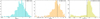 |
Fig. 1 Histograms of the AMP, NEV, and SCATT_LO distributions in logarithmic scale for the sources released in the catalogue. Negative values are excluded. Vertical lines are thresholds for sources considered significantly variable. More details are given in Sect. 5.1. |
5 Results
In Sect. 5.1 we describe how the DR1 variability catalogue was built, and this is followed by a section dedicated to the cross-match with existing catalogues of X-ray sources (Sect. 5.2), a description of the classification of the optical counterparts (Sect. 5.3), and the description of the catalogue data model (Sect. 5.4). We conclude with a description of the most variable eRASS1 sources in Sect. 5.5.
At the end of this section, we provide notes on cataclysmic variables (Sect. 5.6), notes on the stellar sources in the eRASS1 variability sample (Sect. 5.7), notes on X-ray binaries (Sect. 5.8), and notes on AGN in the eRASS1 variability sample (Sect. 5.9).
5.1 The eRASS1 variability catalogue
We applied the three tests to all the 128 669 sources that have at least ten net counts and for which eSASS provided a light curve, over the entire DR1 catalogue, after excluding an area of radius 4.25 degrees, centred on the South Ecliptic Pole (SEP). This region has the highest number of visits and the deepest data, which needed a dedicated analysis, presented in Bogensberger et al. (2024) and Liu et al. (in prep.).
Applying to this sample the criteria described in Sect. 4 we retained:
A number of 808 sources with AMPσ > 0, 90 of which are significant according to the threshold AMPσ > 2.6 of B2022.
A number 298 sources with NEVσ > 0, 123 of which are significant according to the NEVσ > 1.7 threshold of B2022.
A further 1342 sources found with the Bayesian excess variance test for SCATT_LO whose values are greater than 0.14 B2022.
The distribution of positive AMPσ, NEVσ, and SCATT_LO values is shown in Fig. 1.
Sources from DR1 are considered significantly variable if their AMPσ values are greater than 2.6, their NEVσ values are greater than 1.7, or their SCATT_LO values are greater than 0.14 (as indicated by the dashed vertical lines in Fig. 1.) These thresholds were derived in B2022 (see his Section 4.1) from enforcing a 3σ-equivalent significance at multiple count rates simultaneously, which resulted in a sample false positive rate that is orders of magnitude lower than 0.3%. Dividing the expected number of false positives in Table 2 of B2022 by their parent sample size of 27910, they estimate a false positive rate of 0.0004% for AMP and NEV, 0.05% for the Bayesian excess variance.
Scaling the false positive rates from that study to our parent sample size, we expect fewer than 1 false positives from AMP and NEV and 61 false positives from Bayesian excess variance. Sources below these thresholds are candidate variable sources and will be further tested with deeper follow-up X-ray observations.
The total number of unique sources is 1709, and they form the catalogue of variable sources released with this paper. The breakdown of the sources among the criteria is shown by using the UPSET4 tool for the visualisation of intersecting samples (Lex et al. 2014) is shown in Fig. 2. Only 24 of the 1709 sources are considered variable by the three most stringent criteria simultaneously, while 201 are in common considering the more relaxed definition, and 285 are in common to two tests.
As discussed in B2022, the different tests are complementary; for example, the Bayesian excess variance performs best in the low count regime with 900 sources classified as variable only by this method, while the AMP test excels at identifying flares. In this work, five variable sources are identified only through AMP. Interestingly, the diagram shows that all the sources with NEV>0 and the majority of those with AMP>0, are also classified as varying by at least another method.
Finally, in Fig. 3 we show the dependence of the source count rates on the significance of variability according to the tests NEV, AMP, and the Bayesian excess variance, respectively. To search for trends, we defined groups in count rates (with bin edges: 0.1, 1, 10, 100, 1000 cts/s). For each group, the mean statistic and its uncertainty are shown by the black error bars in Fig. 3. To test for any significant trend, we test whether these groups share the same mean with an ANOVA test. AMPσ (p-value < 0.001) and NEVσ (p=0.008) show a positive trend, while SCATT_LO does not. This is because the NEV and AMP tests are most sensitive when the error bar sizes are smallest at high count rates, while the Bayesian excess variance method also performs well in the Poisson regime. The number of variable sources is less than about 1% of the complete DR1 catalogue.
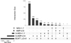 |
Fig. 2 Breakdown of the catalogue of variable sources according to the three tests of variability applied: NEV, AMP, and bexvar. For NEV and AMP, we applied two thresholds: NEV > 0 σ and AMP > 0 σ indicate sources with some indication of variability; NEV > 1.7 σ and AMP > 2.6 σ indicate sources that are variable with good confidence. For bexvar we used a single threshold, SCATT_LO>0.14, that indicates confident variable sources. Out of the 1709 unique sources that comprise the catalogue, only 24 meet all three stringent thresholds. (For more details, see Sect. 5.1). |
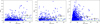 |
Fig. 3 Distributions of AMPσ (left), NEVσ (middle), and SCATT_LO (right) as a function of count rates. The horizontal solid green lines indicate our significance cuts, and dashed lines indicate preliminary cuts. The black error bars show the mean and standard deviation in four logarithmically spaced bins. See more discussion in Sect. 5.1. |
5.2 Cross-matches with existing catalogues
In recent years, many wide-area and all-sky source catalogues have been generated at any wavelength, allowing us to identify and possibly characterise the eROSITA sources in the variability catalogue. We have performed cross-matches with various source catalogues following two approaches: one matching eROSITA sources to those in other X-ray catalogues and another matching the most likely multi-wavelength eROSITA counterpart to catalogues of specific sources to characterise their nature.
Concerning the cross-match with existing X-ray catalogues, this allowed us to verify whether or not the eROSITA DR1 variable sources are already known to be X-ray emitters. For that, we matched the eROSITA DR1 variable sources to XMM-Newton (4XMM_dr13) (Webb et al. 2020), 2RXS (Boller et al. 2016), 2SXPS (Evans et al. 2020), and Chandra/CSC2.1 (Evans et al. 2024), adopting a radius search of 15″ (e.g. about three times the median positional error of eROSITA). We have identified 258, 318, 598, and 79 sources in the 4XMM DR13, 2SXPS, 2RXS, and CSC2.1 catalogues, respectively. Figure 4 shows the sources in common to the various catalogues using the same tool used in Fig. 2. Only 27 sources are common to all catalogues, and 882 sources (51.5%) of the eROSITA DR1 variability catalogue are new detections. However, one should not forget that among the tree catalogues used for the comparison, only 2RXS (Boller et al. 2016) is an all-sky survey. In addition, the match is done considering only the closest sources to the eROSITA one, and it cannot be ruled out that the match is a chance association, also due to the variable nature of the sources at these wavelengths, and due to the low angular resolution of eROSITA. A more detailed analysis is needed to verify that the association between different X-ray catalogues is correct.
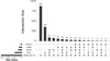 |
Fig. 4 Diagram representing how the 1709 eROSITA DR1 candidate variable sources are distributed among the 4XMM DR13, 2RXS, 2SXPS and CSC2.1 catalogues. 882 (52%) of the sources are new detections by eROSITA. The empty intersections are not shown. |
5.3 Classification of the optical counterparts
For the characterisation of the sources (star/galaxy classification, which type of star or AGN, etc.), we first relied on the identification of the multi-wavelength counterpart to the entire eROSITA/DR1 catalogue (Merloni et al. 2024) presented in (Freund et al. 2024) and Salvato et al. (in prep.). This shift from eROSITA to the counterparts’ optical coordinates significantly reduces the chance of association with existing catalogues of sources or databases such as SIMBAD (Wenger et al. 2000). The drawback is that in the match, it is assumed that the counterpart presented in those papers is the correct one. However, both papers exhaustively discuss the probabilities of associations and chance probabilities.
In Freund et al. (2024), the authors are hunting for coronal stars and use a Bayesian algorithm, Hamstar, to determine the most likely coronal star associated with an eROSITA source. The associations are expected to be reliable at 90% level on average, but increase for sources with high detection likelihood, as for the sources in the eROSITA DR1 variability catalogue (DET_LIKE_0>20) presented here. Using the Freund et al. (2024) catalogue, we found that 1192 (69.7%) of the eRASS DR1 variable sources are classified as coronal stars. While in Freund et al. (2024) the goal was to identify coronal stars, in Salvato et al. (in prep.), the goal was to identify the counterpart of all eROSITA sources, regardless of their Galactic or extragalactic nature. For that, the authors have used NWAY (Salvato et al. 2018), a Bayesian algorithm that assigns the most likely counterpart, accounting for separation between sources in the primary (X-ray) and secondary (optical) catalogues, their positional uncertainties and number densities, and enhanced by a prior. The prior was defined using a training sample of X-ray emitters (stars, compact objects, AGN, QSO) with secure counterparts from XMM-Newton and Chandra. Also for this catalogue, the associations are reliable in more than 90% of the cases and increase at high detection likelihood.
Using this second catalogue, we find that 1678 (98.2%, that is 30% more than with the coronal stars catalogue) of the sources in our sample are reliably associated to a Gaia counterpart. It is reassuring that the 1192 sources in Freund et al. (2024) have the same counterparts identified in the Salvato et al. catalogue. For each source, Gaia provided the probability to be a star (P_star), a galaxy (P_Gal) or a QSO (P_QSO). These probabilities were obtained with a combination of various machine learning algorithms applied to mean BP/RP spectra (Creevey et al. 2023; Fouesneau et al. 2023; Delchambre et al. 2023). We find that 72.7% of the sources are classified as stars with a probability pStar>50%, 4.6% has pQSO>50%, and 1.6% are considered to be galaxies (pGal>50%). For the latter, the source of the X-ray emission could be from a low luminosity AGN or from ULXs. Both interpretations would explain the X-ray variability. Figure 5, shows the distribution of the Gaia counterparts in the BP-G vs. G-RP plane, with the breakdown for each class. The arc structure on the bottom right is the locus of the stars, where indeed most of our sources are. The diagonal distribution is the locus of extragalactic sources (see Fig. 5 of Bailer-Jones et al. 2019). For completeness, we also cross-matched the counterparts to the Veron & Veron AGN Catalogue (Véron-Cetty & Véron 2010) for which we found a match for 71 QSO, assuming a maximum separation of 3″5.
For the 181 sources, the counterpart is identified in Gaia, but the classification is not provided. For those, we looked at their Wise W1-W2 catWISE2020 (Marocco et al. 2021) colours and found that 166 have colours consistent with those of Galactic stars (Stern et al. 2012, W1 − W2 ~ 0;). In summary, only 10% of the 1708 sources forming our catalogue are associated with extragalactic sources. We attempted to further classify the stellar component by looking at the LMXB (Liu et al. 2001), HMXB (Fortin et al. 2023), Yale Bright Star (Hoffleit & Jaschek 1991) and CVs (RKcat; Ritter & Kolb 2003) catalogues. More details on the matches to these catalogues of a specific type of sources are presented in Sect. 5.5.
 |
Fig. 5 Gaia colour-colour plot of the optical counterparts associated with the eROSITA sources in the eRASS1 variability catalogue. The classification of the sources as Galactic or extragalactic follows Sect. 5.3. Most of the sources are classified as coronal stars from Freund et al. (2024), while for the remaining sources identified in Salvato et al., in prep., the classification is derived from the Gaia properties listed in the original catalogue with a probability of being galaxies, QSOs, or stars higher than 50%. Few sources are classified as star or AGN based on their WISE colours or as QSO based on the Veron & Veron catalogue. Most of the sources are stellar, and only 10% of the sources are classified as of extragalactic nature. |
5.4 eROSITA DR1 variable source catalogue data model
The catalogue includes the unique IAU name, eROSITA source identifier (DetUID), and the prefix of associated filenames of the DR1 data sets (filename) along with the eROSITA equatorial, ecliptic and Galactic coordinates. We provided the standard output values from the eSASS analysis software, for example, the list of source and background net count rates. Additionally, we list the variability results for each of the applied tests (AMP, NEV, SCATT_LO) and the significance of AMP and NEV. The coordinates of the optical counterpart are also provided. The key information of the catalogues listed in Sect. 5.2, for example 4XMM_dr13, 2RXS, 2SXPS and CSC2.1, are also kept. Finally, the most likely nature of the source (Galactic, extragalactic) is reported, together with the IDs in the original catalogues of LMHB, HMXB, CVs, if available.
5.5 The most variable eRASS1 sources
In Fig. 6 and Table 1, we present the 12 most variable sources within eRASS1, ranked according to the larger value between AMPσ and NEVσ, including their best known object ID, using the Gaia identification of the sources, as presented in Sect. 5.2. Subsequently, we provide a list of variability characteristics, object identifications, and pre-eROSITA X-ray timing properties. Ideally, we would like to provide a spectral analysis for all the sources, but for most of them across the various classes, the number of counts is insufficient. The DR1 catalogue paper (Merloni et al. 2024) adopts a standard energy conversion factor based on an AGN with a photon index of 2 under a Galactic column density of 3 × 1020 cm−2, which for 0.6–2.3 keV gives 5.253 × 1011 cm2/erg. This allowed us to convert the count rates shown in this paper to fluxes.
Some of the brightest stellar flares have sufficient counts to characterise the temperature and luminosity of the plasma. When possible, we fit the data with the flare spectroscopy method, described below.
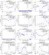 |
Fig. 6 Light curves of the 12 most variable DR1 sources. The bin size is one eroday, and the energy range is (0.6–2.3) keV. For the normalised excess variance and the maximum amplitude variability, the values and significance (NEVσ, AMPσ) in units of σ are indicated along the top of each panel. As in Table 1, the objects are ordered by significance (NEVσ or AMPσ, whichever is larger) from top left to bottom right. The Bayesian excess variance is also indicated (SCATT), with the 10% (bottom, SCATT_LO) and 90% quantiles (top). The IAU name is given at the top of each figure. The x-axis shows the time in MJD units normalised to the launch of eROSITA on 2019-12-11, 21:30 (GMD) in days. The large variability of GX 339–4 is interpreted as due to pile-up (cf. Sect. 5.5.2.). |
List of the most variable eRASS1 sources, sorted by the larger value between NEVσ and AMPσ.
5.5.1 Flare spectroscopy
We fit the DR1 X-ray spectrum following the M dwarf flare analysis method6 of Rukdee et al. (2024). This is based on the Astrophysical Plasma Emission Code APEC model (Smith et al. 2001). Briefly, instead of a one or two-temperature model, Rukdee et al. (2024) adopted a source model with a log-Gaussian Differential Emission Measure (DEM) distribution, where the mean temperature kTpeak, standard deviation σlog T, peak normalisation and metal abundance are free parameters, with wide prior ranges. Galactic absorption is modelled with TBabs (Wilms et al. 2000) using column densities taken from NH3Dtool7 (Doroshenko 2024) based on the map of Edenhofer et al. (2024). The spectral fitting is performed with Bayesian X-ray Analysis (BXA; Buchner et al. 2014), which connects the nested sampling (Skilling 2004; Buchner 2023) algorithm MLFriends (Buchner 2016, 2023) implemented in the UltraNest package (Buchner 2023) with the fitting environment CIAO/Sherpa (Fruscione et al. 2006). The background spectrum is modelled with the PCA-based model of Simmonds et al. (2018), as previously described in Liu et al. (2022), and the background normalisation is fitted simultaneously with the source parameters. We assume Poisson (C-Stat) statistics.
5.5.2 GX 339–4
GX 339–4 is the most variable LMXB (1eRASS J170249.6–484725), one of the most well-known and thoroughly investigated LMXBs, at a distance of about 8.4 kpc (e.g., Parker et al. 2016). Extensive studies have been carried out to understand state transitions, exploring changes in the shape of the X-ray spectrum, the onset of timing variability patterns, shifts in luminosity, and movements of the inner radius of the accretion disc, as demonstrated by examples such as Tananbaum et al. (1972); Droulans et al. (2010), and Shui et al. (2021).
Despite the source being classified as variable in eROSITA, the simultaneous light curve from MAXI suggests a non-significant variability as shown in Fig. 7. This difference in the light curves may suggest that the variability detected by eROSITA is instrumental and could be due, for example, to the pile-up effect. This effect is generated when two or more photons hit the same CCD pixel in the same (50 ms) read-out cycle. More details about the process related to eROSITA are presented in Merloni et al. (2024), and a practical example is presented by König et al. (2022) for the observation of YZ Reticuli, in eRASS2. Preliminary studies using SIXTE (Dauser et al. 2019) indicate that for eRASS1, pile-up starts to become important (more than a few percent effect) for point sources brighter than 10−11 erg cm−2 s−1 in the 0.2–2.3 keV band. GX 339–4 has a flux in this band of 5.48 × 10⁻¹⁰ erg cm−2 s−1.
5.5.3 GRB 200120A
The second most variable source is the X-ray afterglow of the gamma-ray burst GRB 200120A detected with Fermi/GBM (Hamburg et al. 2020). On UTC Jan 20th, 2020, at 23:18:15 (820 s after the Fermi/GBM trigger) Weber (2020) reported a detection with eROSITA/SRG of a bright and quickly fading X-ray source. The actual length of the afterglow observations in the eRASS1 all-sky survey is about 40 s, as indicated in Fig. 6, with an average flux over the period of 1.72 ± 0.05 × 10⁻¹² erg s−1 cm−2. The object 1eRASS J090827.6–702615 exhibits the highest NEV significance value of all DR1 sources, with NEV = 13.39 σ.
5.5.4 Cen X–3
The third most variable source is the HMXB Cen X–3 (1eRASS J112114.8–603723). Cen X–3 is the first X-ray pulsar discovered (Giacconi et al. 1971) and has been extensively studied at X-rays to constrain the pulse phase, magnetic field structure, and disc precession (Iping & Petterson 1990; Burderi et al. 2000; Ji et al. 2019). The light curve is relatively flat with a slightly increasing slope, interrupted by a 50 ks-long gap where the flux decreased by two orders of magnitude. Another similar decrease is seen at the end of the light curve. The averaged eRASS1 flux is 7.8 ± 0.8 × 10⁻¹¹ erg s−1 cm−2.
Cen X–3 has an orbital period of 2.087 days and shows eclipses of the X-ray source by the companion star. Extrapolating the ephemeris for the time of mid-eclipse determined by Klawin et al. (2023) to the times of the eROSITA observations, we derive MJD 58861.039 days, which is fully consistent with the centre of the observed gap. Therefore, the eclipse of the X-ray source clearly explains the gap and the decrease at the end of the eROSITA light curve about 2 days later.
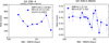 |
Fig. 7 Left panel: eROSITA light curve of GX 339–4 in the soft (0.6–2.3 keV) band. Right panel: MAXI light curve in the (2–4) keV band. The AMP and NEV values obtained from the MAXI light curve are below three σ. The eROSITA AMP and NEV values are 16.77, 12.42 σ (soft 0.6–2.3 keV) and 3.47, 3.81 σ (hard 2.3–5 keV), respectively. The eROSITA soft and hard band DR1 light curves are strongly affected by pile-up (cf. Sect. 5.5.2). |
5.5.5 SMC X–1
One of the first X-ray observations of the HMXB SMC X–1 have been reported by Schreier et al. (1972). The source is part of the Small Magellanic Cloud at a distance of about 60 kpc and has been intensively studied with pointed X-ray observations by, for example, Haberl et al. (2008).
In the first six months of observations, SMC X–1 (1eRASS J125048.1–732630) shows a drop in flux toward the end of the survey due to an eclipse by the B0 supergiant companion. The analysis of the eRASS1,2,3,4 data performed in Sect. 5.8 suggests that the extrapolated eclipse times are slightly too early in phase, compared to previous studies.
5.5.6 G 124–44
The source G 124–44 is classified as an eruptive variable M4 dwarf type (Terrien et al. 2015) at a distance of about 20 pc. During the eRASS1 observations (average flux 7.6 ± 0.2 × 10⁻¹² erg s−1 cm−2), the object is mostly faint with very low count rates, except for a pronounced single flare reaching a count rate of about 40 cts s−1. To measure the flare parameters, we fit the DR1 spectrum, assuming that the flare dominates the source counts. The spectrum is fitted well by the log-Gaussian DEM model (see Sect. 5.5.1) according to a reduced χ2 < 1 after rebinning to 50 counts per bin. We find an abundance of Z = 0.21 ± 0.06Z⊙. The DEM peaks at 3.15 ± 0.95 keV with a standard deviation of 0.67 ± 0.16 dex. Such high energies are typical for flares (Robrade & Schmitt 2005). The flare energy is three times higher than that seen in the LTT1445A flare (Rukdee et al. 2024) with an identical analysis, possibly related to that flare being 15 times less luminous: We find a Galactic absorption-corrected flare 0.5–2 keV flux of 5.57 ± 0.17 × 10⁻¹² erg s−1 cm−2, which corresponds to a luminosity of LX = 3.16 × 1028 erg s−1. The flare is poorly sampled, but if we conservatively assume a flare duration of 40s, we obtain a lower limit of the flare energy of 1030 erg.
5.5.7 El Eridani
The object is located at a distance of 54 pc and is classified as a variable star of RS CVn-type binaries and has been extensively studied at X-rays with XMM-Newton pointed observations by Pandey & Singh (2012). Fig. 6 shows its light curve. The source is already in its pre-flare phase, bright with about 20 cts s−1 that covers the initial 40 ks, which is followed by an increase up to 100 cts s−1 and a subsequent decrease in count rate during the remaining eRASS1 coverage. If interpreted as a continuous event, the factor of 5 flare appears to decay over at least 8 hours in the eRASS1 observations.
5.5.8 UCAC4 190–003482
The star (listed in the UCAC4 catalogue; Zacharias et al. 2012)8 has a distance of 25.8 pc and is classified as a red dwarf. To our knowledge, it was not previously detected in X-rays. The star shows a strong increase up to 30 counts s−1 in the last eroday. Before that, the light curve shows very low activity below 2 counts s−1, indicating a phase of inactivity (see Sect. 5.7). We quantify the flare spectroscopically as described in Sect. 5.5.1. The abundance is Z = 0.59 ± 0.22Z⊙. Similar to G 124–44, the DEM distribution peaks at 3.14±0.98 keV with a width of 0.62±0.20 dex. This gives a flux of 0.50 ± 0.04 × 10⁻¹² erg s−1 cm−2, which corresponds to a luminosity of LX = 2.82 × 1027 erg s−1. The flare is likely not fully sampled by eROSITA. If we conservatively adopt a flare duration of 40 s, we obtain a lower limit for the flare energy of 1029 erg.
5.5.9 GR Mus
GR Mus is an LMXB (Qian et al. 2006). The light curve shows erratic behaviour with highly significant increases and decreases. Towards the end of the light curve, three data points with a two orders of magnitude decrease in flux are seen. No data points are available from the immediate scans before, so this behaviour lasted at least two erodays (8 hours) and recovered to the original flux levels within another 8 hours.
GR Mus (also known as XB 1254–690) has an estimated distance between 8 and 13 kpc (Motch et al. 1987), and it is known to show dipping behaviour in X-rays, which regularly repeats with a period consistent with the orbital period (~3.9 hours) of the binary system. However, the dips vary in duration and depth and can disappear completely (see Díaz Trigo et al. 2009, and references therein). A precessing accretion disc has been discussed as the possible origin of the variability (Cornelisse et al. 2013). The orbital period of the LMXB is close to the eROSITA scanning period of 4.0 hours (resulting in a beat period of ~10 days; for other examples of beat effects with the regular eROSITA sampling see Sect. 5.6). Therefore, the three low-flux measurements were taken at a similar orbital phase and do not necessarily indicate a continuous period of low flux. We suggest that the low fluxes were caused by deep dips that repeated over three consecutive binary orbits. We cannot say how many orbits in total the dips were present, because due to the slow phase drift, the high-flux data would then be taken outside dip phases. We conclude that the eROSITA light curve is consistent with the behaviour seen from this source before, with deep dips seen over consecutive binary orbits. The eRASS1 catalogue lists the average flux over the period shown in Fig. 6 as 8.7 ± 1.3 × 10⁻¹¹ erg s−1 cm−2.
5.5.10 Cir X–1
The HMXB Cir X–1 has been studied with EXOSAT (Tennant et al. 1986) to constrain the X-ray outburst characteristics, and physical mechanisms have been investigated by Blumenthal & Tucker (1972). The source was bright during the eRASS1 observations, with a pronounced drop during the last eroday. Cir X–1 is known to switch between high and low X-ray states (e.g. D’Aì et al. 2012). The eROSITA light curve may indicate an ingress into such a low state within 4 hours, but no further constraints can be derived. The eRASS1 catalogue lists the average flux over the period shown in Fig. 6 as 1.5 ± 0.1 × 10⁻¹⁰ erg s−1 cm−2.
5.5.11 Gaia DR3 3918904293185534080
The Gaia counterpart to this X-ray source has a high proper motion9, at a distance of 59.74 pc. This is the first X-ray detection of the source. The eROSITA discovery light curve shows a strong flare lasting for one eroday, followed by a decline in the X-ray count rate values towards the end of the observations. This is similar to K/M dwarfs found in eFEDS (Boller et al. 2022). However, Gaia does not provide type information on the source. When quantifying the flare spectroscopically, we find an abundance of Z = 0.46 ± 0.12Z⊙. Similar to the other two stars before, the DEM distribution peaks at 3.81 ± 0.74 keV with a width of 0.55 ± 0.08 dex. This gives a flux of 9.33 ± 0.28 × 10⁻¹² erg s−1 cm−2, which corresponds to a luminosity of LX = 5.37 × 1028 erg s−1. If we crudely adopt a flare duration of 4 h, assuming that the peak was sampled and the subsequent light curve data point in Fig. 6 is elevated because it traces the end of the flare, we obtain a flare energy of 7 × 1032 erg.
5.5.12 1ES 1210-64.6
The source 1ES 1210-64.6 is an HMXB, which has also been detected at hard X-rays (17–60 keV) with INTEGRAL (Krivonos et al. 2010). The object, with a distance of about 1 kpc, has been studied with different X-ray satellites (Masetti et al. 2009; Coley et al. 2014). At the start of the eRASS1 observations, count rates are consistent with zero. Then the source shows an impressive X-ray flaring event lasting over about tenerodays, reaching up to about 25 counts s−1. At the end of the eRASS1 observations, the rate decreases to a few counts per second. The eRASS1 catalogue lists the average flux over the period shown in Fig. 6 as 1.63 ± 0.03 × 10⁻¹¹ erg s−1 cm−2.
5.5.13 CD–38 11343
CD–38 11343 is classified as an eruptive variable star and previously detected in the 2RXS catalogue (Boller et al. 2016). It is an M3Ve + M4Ve binary system of flare stars (Tamazian & Malkov 2014). The 2RXS light curve does not show any significant variability, and a spectral fit with an optically thin metal emission model gives a temperature of 0.83 ± 0.10 keV. During the eRASS1 observations one pronounced flare has been detected with a peak count rate of about 30 counts s−1. The eRASS1 catalogue lists the average flux over the period shown in Fig. 6 as 2.13 ± 0.05 × 10⁻¹¹ erg s−1 cm−2.
5.6 Notes on cataclysmic variables in the eRASS1 variability sample
CVs are semi-detached binaries with white dwarfs that accrete matter via Roche-lobe overflow from low-mass, main-sequence stars (Warner 1995). They were found in reasonably large numbers by their optical variability through nova and dwarf nova outbursts, by their blue colour in objective prism surveys, spectroscopically in the SDSS as quasar candidates, and as counterparts to point-like X-ray sources (Gänsicke 2005). Indeed, all CVs have in common that they are X-ray sources. This property allows for the composition of flux-limited samples and will eventually allow for the composition of volume-limited samples to constrain close binary evolution (Schwope et al. 2002, 2024). The accretion process in CVs generates intense X-ray emission, characterised by variability over a wide range of timescales. This variability is key to understanding the dynamics of the accretion flow and the interactions between the white dwarf and its environment. We found 16 sources matched to the CVs catalogue of Ritter & Kolb (2003). The sources can be subclassified as ten-magnetic CVs (5 intermediate polars, 5 polars), 5 dwarf novae (2 SU UMa, 2 U Gem, 1 Z Cam subtype), and one non-magnetic nova-like object of the VY Scl subtype. All but two were formerly detected in 2RXS. The prevalence of the magnetic objects in the small sample is due to their intrinsic short-term variability on the orbital or the spin period of the accreting white dwarfs.
The observed pattern in the light curves reflects the folding of the intrinsic variability with the sampling period of the spacecraft. Intrinsic variability happens during the orbital period and is caused by eclipses, self-eclipses and perhaps other geometrical effects, plus variations in the instantaneous mass accretion rate, which may give flares or at least non-repetitive brightness at a given spin or orbital phase. The sampling pattern may thus lead to irregular and, in some cases, very regular brightness variations in DR1.
A nice example of a regular light curve with a simple on-off pattern is that of 1eRASS J031130.6–315250 an AM Herculis star or polar with a binary orbital period of ![Mathematical equation: $\[0_\cdot^\mathrm{d}05872\]$](/articles/aa/full_html/2025/08/aa49355-24/aa49355-24-eq15.png) . The DR1 light curve is shown in Fig. 8.
. The DR1 light curve is shown in Fig. 8.
The implied DR1 period of about 24 hours is much longer and likely occurs on some beat frequency between the orbital period of the CV and the scan period of the SRG spacecraft (see Maitra et al. 2024, for another striking example of such an apparent long-period variability of an ultra-compact double degenerate binary). While a quantitative variability analysis and period search could be performed, the light curve shows only two humps, making the result highly unreliable. The scanning pattern mentioned is a further complication. Therefore, we defer to follow-up studies to quantify the significance and period.
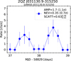 |
Fig. 8 DR1 light curve of 1 eRASS J031130.8-315250 (aka 2 QZ J031130.9-315250) as an example of a typical light curve with a simple on-off pattern of an AM Herculis star or polar with a binary orbital period of |
![Mathematical equation: $\[0_\cdot^\mathrm{d}05872\]$](/articles/aa/full_html/2025/08/aa49355-24/aa49355-24-eq14.png)
5.7 Notes on stellar sources in the eRASS1 variability sample
Stellar sources are the majority of the observed X-ray variable sources (see Fig. 5) and contribute substantially to the number of sources discussed in this work. Especially coronal emitters that generate X-rays by magnetic activity are known to be highly variable and, as detailed in Sect. 5.2, 69% of the sources presented here are identified as coronal stars in the catalogue of Freund et al. (2024). The most extreme luminosity and energy among the three stellar flares analysed here are still within the range of flares found in eFEDS (Boller et al. 2022), although the eROSITA time sampling likely prevents capturing the full flare.
Many flaring stars, young active stars, and active binaries such as RSCVn systems are found to be among the most variable sources. Several add to the list of the most variable eRASS sources reported in Table 1. Exemplary light curves of stellar sources are shown in Fig. 6, and some prominent examples are discussed below. Judging from the ‘object type’ as given in the SIMBAD database and their Gaia colours, nearly half of the significantly variable stars are M dwarfs; in addition 10–20% are classified as very young or pre-main sequence stars and a similar fraction as multiple systems or active binaries. Roughly another 10% belong to other types of variable stars, and some sources are unclassified, apparently ordinary main-sequence stars.
The most variable stellar object is the RSCVn variable V* EI Eri (see Sect. 5.5.7), while the second most variable stellar object is the eruptive variable star G 124-44 (see Sect. 5.5.6). During the eRASS1 observations, the object is mostly faint except for a pronounced single flare.
A similar event is seen on UCAC4 190-003482, which remained inactive throughout the eRASS1 observations except for the last eRASS scan, where it exhibited a sudden brightness increase, reaching a count rate of 30 cts s−1. These burst-like, strong but short flaring events typically occur on timescales of minutes up to an hour and thus mostly produce highly elevated count rates in single eRASS scans (see Fig. 6). Late-type stars, such as the ones shown here, M dwarfs, are frequently identified as their originating sources.
Flaring and active periods may also be present for longer timescales of hours to days. The star 2MASS J12100301+121507 (Gaia DR3 3918904293185534080), a mid-M dwarf at a distance of 60 pc, shows an extreme flare with rates up to 25 cts s−1 that lasts for several hours and is still declining at the end of its survey coverage. Another example among the most variable DR1 objects is the nearby M dwarf binary CD-38 11343 (GJ 2123) at 16 pc distance. It is a bright, variable X-ray emitter as shown by its light curve in Fig. 6.
These findings on stellar variability are similar to those from the eFEDS variability search of Boller et al. (2022) or those described in a detailed analysis of the eROSITA field-scan on the η Chamaeleontis cluster given by Robrade et al. (2022). The variability discussed there is likewise associated with flaring due to magnetic activity in late-type stars, which dominate the X-ray stellar variability. Notably also several early-type stars also exhibit distinct X-ray variability. While in ’normal’ O/B stars, X-ray emission, which is attributed to wind-shocks, is rather constant, massive stars are diverse and more variable sub-categories exist. However, due to their faintness, lower amplitudes and longer timescales, they are basically absent in this work. A systematic eROSITA survey of Be stars by Nazé & Robrade (2023) presents several examples of eRASS variability on scan (4 h) as well as survey (0.5 yr) timescales.
5.8 Example of eRASS1 X-ray variability for X-ray binaries: the case of SMC X–1
The large AMP value obtained for the HMXB SMCX–1 is caused by a drop in flux in the last data point of the eRASS1 light curve (see Fig. 6). In SMC X–1, a neutron star orbits a B0 supergiant, which eclipses the X-ray source regularly every 3.89 days, the binary orbital period of the system (Falanga et al. 2015). Using the ephemeris from Falanga et al. (2015), we obtain an orbital phase of −0.0505 (phase 0 corresponds to mid-eclipse time) for the time of the last eRASS1 scan and −0.0933 for the scan before (which is still at the pre-eclipse flux level).
To investigate this further, we did a detailed analysis of the complete eROSITA data of SMC X–1 from eRASS1-4. To create light curves and spectra, we extracted events from circular regions around the source and a nearby background region. Because of the source brightness, we chose a sufficiently large circle with 2′ radius. The four eRASS spectra were simultaneously fitted by an absorbed two-component model, comprising a power law and diskbb emission. The derived unabsorbed fluxes were used to convert the count rates to X-ray luminosities, assuming a distance of 65 kpc. Figure 9 shows the X-ray luminosity versus time in Modified Julian Date (MJD). Similarly to eRASS1, also the last eROSITA scans of eRASS4 fall near the eclipse ingress of SMC X–1. Falanga et al. (2015) have derived eclipse times and durations for eclipse ingress and egress from hard X-ray observations (17–40 keV), which do not suffer from photo-electric absorption effects. In Fig. 9 we mark the expected times for the start of eclipse ingress (green dashed lines) and the start of the full eclipse (dash-dotted green lines) using again the ephemeris from Falanga et al. (2015). Their uncertainties are less than 2.6×10⁻⁴ days and negligible. During eRASS1, the last two data points of the light curve are fully consistent with the eclipse ingress between them. During eRASS4, the last but one point falls into the expected hard X-ray ingress period, which may indicate a start of the full eclipse slightly earlier than predicted by the ephemeris. However, at lower X-ray energies (eROSITA is most sensitive between 0.5 and 2 keV), the eclipse is less sharp and the low luminosity could also be explained by strong absorption effects often seen at these orbital phases. Unfortunately, no egress was covered, and given the uncertain eclipse duration in the eROSITA energy band, no further constraints can be derived.
 |
Fig. 9 eROSITA light curves of SMC X–1. Count rates were converted into X-ray luminosity using parameters from spectral modelling. The vertical dashed and dash-dotted green lines mark the orbital phases of the expected start of eclipse ingress and start of full eclipse, respectively (see Sect. 5.8). |
5.9 Notes on AGN in the eRASS1 variability sample
As mentioned, about 11% of the DR1 variable sources are classified as AGN. This is in line with the AGN fraction of variable sources found in the eFEDS survey (Boller et al. 2022), which probed similar time-scales of hours at deeper exposures with the same soft X-ray instrument. The variability of AGN shows a bending powerlaw power spectrum, in analogy to that of X-ray binaries (e.g. McHardy et al. 2006; Ponti et al. 2012). Various models for short-term AGN variability have been proposed, e.g. the light bending model (Miniutti & Fabian 2004), the hot spot model (Boller et al. 1997), or the Bardeen-Petterson effect (Bardeen & Petterson 1975). In addition, the coupling of the X-ray corona to the UV radiation from the disc can propagate other sources of variability (e.g., Papadakis et al. 2001; Arévalo & Uttley 2006). These models cannot be tested in detail with the DR1 survey data and require longer pointed observations. Future studies, including all the eROSITA data, are required to test these models (Boller et al. 2016; Buchner et al. 2022). The black hole mass accretion rate is partially converted to radiation with the radiative efficiency η. A variable emission region of mass M is limited to releasing energy ΔLΔt < Mc2. Considering the light travel time and optical depth, gives (Cavallo & Rees 1978; Fabian 1979):
![Mathematical equation: $\[\Delta L / \Delta t<1.6 \times 10^{41}(\eta / 0.1) ~\mathrm{erg} \mathrm{~s}^{-2}.\]$](/articles/aa/full_html/2025/08/aa49355-24/aa49355-24-eq16.png)
As a pilot study, we search for the presence of such strong rapid flux changes in the two most variable AGN, considering their redshift. They do not violate this limit.
The most variable AGN in our sample is PKS 0558–504 with AMP of 3.45σ and NEV of 1.97σ. The source shows a drop in count rate by a factor of about three within about 15 000 seconds. PKS 0447–439 shows variations by a factor of up to 2 during the eRASS1 observations. The AMP and NEV are 2.18σ and 2.21σ, respectively (see Fig. 10).
6 Summary
We selected 128 669 sources with at least tencounts out of DR1, after excluding an area of about 226 square degrees centred on the SEP. We systematically searched for variability in the light curves of the sources using three types of tests: bexvar, AMP and NEV (see Sect. 4). According to bexvar 1342, sources are variable, while 808 are considered varying by AMP and 298 by NEV. The total number of unique sources is 1709, and they form the catalogue of variable sources. The total number of variable sources is less than about 1% of the complete DR1 catalogue.
Using more stringent thresholds for AMP and NEV (B2022), only 90 sources demonstrated significant variability via AMP, while 95 did so through NEV. Both subsamples are classified as variable by bexvar, but only 69 sources are in common to all criteria (see Fig. 2). We have performed cross-matches with existing X-ray catalogues. We have identified 258, 318, 598, and 120 sources within 15″ have a counterpart in 4XMM DR13, 2SXPS, ROSAT/2RXS, and CSC2.1 catalogues. However, a more detailed analysis is required to asses whether these are the same sources or not. Only 27 sources are common to all of these catalogues, and 882 sources (52%) of the eROSITA DR1 variability catalogue are new X-ray detections.
Using the catalogues of multi-wavelength counterparts of Salvato et. al. (in prep) and Freund et al. (2024), we classified the sources using existing catalogues of LMXB, HMXB, QSOs, etc. About 10% of the sources are extragalactic (AGN and QSO) while 89% are Galactic, with 70% classified as coronal stars. We have further classified the stellar component into LMXB, HMXB, and Bright stars and found a match for 18, 11, and 14 sources, respectively.
We have described in more detail the 12 most variable eRASS1 sources by providing light curves and statistical test results, as well as results obtained for these sources with other X-ray observations. We provide additional descriptions for some subclasses in the eRASS1 variability sample. Magnetically active stars are commonly found among the more variable X-ray sources, and often, burst-like flare events are seen from otherwise faint or undetected objects. Examples include the star UCAC4 190-003482 that remained inactive throughout the eRASS1 observations except for the last data point, where it exhibited a sudden increase, reaching a count rate of 30 cts s−1 or the M dwarf G 124–44 where a similar event was detected. As an example of X-ray variability for X-ray binaries, we describe the case of SMC X–1 as detected during the eRASS1 observations. Finally, we also provide notes on two AGNs in the eRASS1 variability sample: PKS 0558–504 and PKS 0447–439.
In this paper, we have analysed the variability of eRASS1 sources on a timescale of a few days only. To study the physics of variable sources, we need more deeply pointed observations with other X-ray missions or at least the final depth of the eRASS:8 observations. The timescale of the eRASS1 observations is not representative of the timescales of the expected upcoming eRASS catalogues. The DR1 variability catalogue is an excellent resource for follow-up observations with telescopes such as XMM-Newton, Chandra, or Swift.
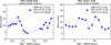 |
Fig. 10 Light curve examples for DR1 sources classified as AGN. The left panel shows the light curve of PKS 0558–504, and the right panel is for PKS 0447–439 (cf. Sect. 5.9). |
Data availability
The full catalogue is available at the CDS via https://cdsarc.cds.unistra.fr/viz-bin/cat/J/A+A/700/A61. The list of columns and their description is presented in the Appendix in the Table A.1.
Acknowledgements
We are grateful for the referee’s detailed report, which greatly enhanced the paper’s quality. This work is based on data from eROSITA, the soft X-ray instrument aboard SRG, a joint Russian-German science mission supported by the Russian Space Agency (Roskosmos), in the interests of the Russian Academy of Sciences represented by its Space Research Institute (IKI), and the Deutsches Zentrum für Luft- und Raumfahrt (DLR). The SRG spacecraft was built by Lavochkin Association (NPOL) and its subcontractors, and is operated by NPOL with support from the Max Planck Institute for Extraterrestrial Physics (MPE). The development and construction of the eROSITA X-ray instrument was led by MPE, with contributions from the Dr. Karl Remeis Observatory Bamberg & ECAP (FAU Erlangen-Nuernberg), the University of Hamburg Observatory, the Leibniz Institute for Astrophysics Potsdam (AIP), and the Institute for Astronomy and Astrophysics of the University of Tübingen, with the support of DLR and the Max Planck Society. The Argelander Institute for Astronomy of the University of Bonn and the Ludwig Maximilians Universität Munich also participated in the science preparation for eROSITA". The eROSITA data shown here were processed using the eSASS/NRTA software system developed by the German eROSITA consortium. MK acknowledges support from DLR FKZ 50OR2307.
Appendix A Catalogue data model
The catalogue includes the key columns of the original eRASS1 catalogue presented in (Merloni et al. 2024), focusing on the 0.2-2.3 keV (medium) band. It also contains columns that describe the variability of the sources as determined in this paper and a list of columns that are the result of the cross-match with existing catalogues. The ID from these catalogues is reported so that for a user, it will be easy to recover additional information. See Table A.1 for the description of the columns.
eROSITA DR1 Variability catalogue column description.
References
- Arévalo, P., & Uttley, P. 2006, MNRAS, 367, 801 [Google Scholar]
- Bahramian, A., & Degenaar, N. 2023, in Handbook of X-ray and Gamma-ray Astrophysics (Berlin: Springer), 120 [Google Scholar]
- Bailer-Jones, C. A. L., Fouesneau, M., & Andrae, R. 2019, MNRAS, 490, 5615 [CrossRef] [Google Scholar]
- Bardeen, J. M., & Petterson, J. A. 1975, ApJ, 195, L65 [Google Scholar]
- Beuermann, K., & Thomas, H. C. 1993, Adv. Space Res., 13, 115 [NASA ADS] [CrossRef] [Google Scholar]
- Blumenthal, G. R., & Tucker, W. H. 1972, Nature, 235, 97 [Google Scholar]
- Bogensberger, D., Nandra, K., Salvato, M., et al. 2024, A&A, 687, A37 [NASA ADS] [CrossRef] [EDP Sciences] [Google Scholar]
- Boller, T., Brandt, W. N., Fabian, A. C., & Fink, H. H. 1997, MNRAS, 289, 393 [Google Scholar]
- Boller, T., Freyberg, M. J., Trümper, J., et al. 2016, A&A, 588, A103 [NASA ADS] [CrossRef] [EDP Sciences] [Google Scholar]
- Boller, T., Schmitt, J. H. M. M., Buchner, J., et al. 2022, A&A, 661, A8 [NASA ADS] [CrossRef] [EDP Sciences] [Google Scholar]
- Brunner, H., Liu, T., Lamer, G., et al. 2022, A&A, 661, A1 [NASA ADS] [CrossRef] [EDP Sciences] [Google Scholar]
- Buchner, J. 2014, Statistics and Computing (Berlin: Springer), 1 [Google Scholar]
- Buchner, J. 2016, Stat. Comput., 26, 383 [Google Scholar]
- Buchner, J. 2023, Stat. Surveys, 17, 169 [NASA ADS] [CrossRef] [Google Scholar]
- Buchner, J., Georgakakis, A., Nandra, K., et al. 2014, A&A, 564, A125 [NASA ADS] [CrossRef] [EDP Sciences] [Google Scholar]
- Buchner, J., Boller, T., Bogensberger, D., et al. 2022, A&A, 661, A18 [NASA ADS] [CrossRef] [EDP Sciences] [Google Scholar]
- Burderi, L., Di Salvo, T., Robba, N. R., La Barbera, A., & Guainazzi, M. 2000, ApJ, 530, 429 [NASA ADS] [CrossRef] [Google Scholar]
- Cavallo, G., & Rees, M. J. 1978, MNRAS, 183, 359 [Google Scholar]
- Coley, J. B., Corbet, R. H. D., Mukai, K., & Pottschmidt, K. 2014, ApJ, 793, 77 [NASA ADS] [CrossRef] [Google Scholar]
- Cornelisse, R., Kotze, M. M., Casares, J., Charles, P. A., & Hakala, P. J. 2013, MNRAS, 436, 910 [NASA ADS] [CrossRef] [Google Scholar]
- Creevey, O. L., Sordo, R., Pailler, F., et al. 2023, A&A, 674, A26 [NASA ADS] [CrossRef] [EDP Sciences] [Google Scholar]
- D’Aì, A., Bozzo, E., Papitto, A., et al. 2012, A&A, 543, A20 [NASA ADS] [CrossRef] [EDP Sciences] [Google Scholar]
- Dauser, T., García, J., & Wilms, J. 2016, Astron. Nachr., 337, 362 [NASA ADS] [CrossRef] [Google Scholar]
- Dauser, T., Falkner, S., Lorenz, M., et al. 2019, A&A, 630, A66 [NASA ADS] [CrossRef] [EDP Sciences] [Google Scholar]
- De Marco, B., Motta, S. E., & Belloni, T. M. 2022, in Handbook of X-ray and Gamma-ray Astrophysics, eds. C. Bambi, & A. Sangangelo (Berlin: Springer), 58 [Google Scholar]
- Delchambre, L., Bailer-Jones, C. A. L., Bellas-Velidis, I., et al. 2023, A&A, 674, A31 [NASA ADS] [CrossRef] [EDP Sciences] [Google Scholar]
- Díaz Trigo, M., Parmar, A. N., Boirin, L., et al. 2009, A&A, 493, 145 [NASA ADS] [CrossRef] [EDP Sciences] [Google Scholar]
- Done, C., Gierliński, M., & Kubota, A. 2007, A&A Rev., 15, 1 [CrossRef] [Google Scholar]
- Doroshenko, V. 2024, A&A, submitted [arXiv:2403.03127] [Google Scholar]
- Droulans, R., Belmont, R., Malzac, J., & Jourdain, E. 2010, ApJ, 717, 1022 [NASA ADS] [CrossRef] [Google Scholar]
- Edelson, R. A., Krolik, J. H., & Pike, G. F. 1990, ApJ, 359, 86 [NASA ADS] [CrossRef] [Google Scholar]
- Edelson, R., Turner, T. J., Pounds, K., et al. 2002, ApJ, 568, 610 [CrossRef] [Google Scholar]
- Edenhofer, G., Zucker, C., Frank, P., et al. 2024, A&A, 685, A82 [NASA ADS] [CrossRef] [EDP Sciences] [Google Scholar]
- Evans, P. A., Page, K. L., Osborne, J. P., et al. 2020, ApJS, 247, 54 [Google Scholar]
- Evans, I. N., Evans, J. D., Martínez-Galarza, J. R., et al. 2024, ApJS, 274, 22 [NASA ADS] [CrossRef] [Google Scholar]
- Fabian, A. C. 1979, Proc. R. Soc. London Ser. A, 366, 449 [Google Scholar]
- Falanga, M., Bozzo, E., Lutovinov, A., et al. 2015, A&A, 577, A130 [NASA ADS] [CrossRef] [EDP Sciences] [Google Scholar]
- Fornasini, F., Antoniou, V., & Dubus, G. 2023, in Handbook of X-ray and Gamma-ray Astrophysics (Berlin: Springer), 143 [Google Scholar]
- Fortin, F., García, F., Simaz Bunzel, A., & Chaty, S. 2023, A&A, 671, A149 [NASA ADS] [CrossRef] [EDP Sciences] [Google Scholar]
- Fouesneau, M., Frémat, Y., Andrae, R., et al. 2023, A&A, 674, A28 [NASA ADS] [CrossRef] [EDP Sciences] [Google Scholar]
- Freund, S., Czesla, S., Predehl, P., et al. 2024, A&A, 684, A121 [NASA ADS] [CrossRef] [EDP Sciences] [Google Scholar]
- Fruscione, A., McDowell, J. C., Allen, G. E., et al. 2006, SPIE Conf. Ser., 6270, 62701V [Google Scholar]
- Fuhrmeister, B., & Schmitt, J. H. M. M. 2003, A&A, 403, 247 [NASA ADS] [CrossRef] [EDP Sciences] [Google Scholar]
- Gänsicke, B. T. 2005, ASP Conf. Ser., 330, 3 [Google Scholar]
- Gehrels, N. 1986, ApJ, 303, 336 [Google Scholar]
- Georgakakis, A., Buchner, J., Ruiz, A., et al. 2024, MNRAS, 531, 4524 [Google Scholar]
- Giacconi, R., Gursky, H., Kellogg, E., Schreier, E., & Tananbaum, H. 1971, ApJ, 167, L67 [NASA ADS] [CrossRef] [Google Scholar]
- Güdel, M. 2004, A&A Rev., 12, 71 [Google Scholar]
- Haberl, F., Eger, P., Pietsch, W., Corbet, R. H. D., & Sasaki, M. 2008, A&A, 485, 177 [NASA ADS] [CrossRef] [EDP Sciences] [Google Scholar]
- Hamburg, R., Meegan, C., & Fermi GBM Team 2020, GRB Coordinates Netw., 27025, 1 [Google Scholar]
- Hessman, F. V., Gänsicke, B. T., & Mattei, J. A. 2000, A&A, 361, 952 [NASA ADS] [Google Scholar]
- Hoffleit, D., & Jaschek, C. 1991, The Bright Star Catalogue (New Haven: Yale University Observatory) [Google Scholar]
- Iping, R. C., & Petterson, J. A. 1990, A&A, 239, 221 [NASA ADS] [Google Scholar]
- Ji, L., Staubert, R., Ducci, L., et al. 2019, MNRAS, 484, 3797 [Google Scholar]
- Klawin, M., Doroshenko, V., Santangelo, A., et al. 2023, A&A, 675, A135 [NASA ADS] [CrossRef] [EDP Sciences] [Google Scholar]
- König, O., Wilms, J., Arcodia, R., et al. 2022, Nature, 605, 248 [CrossRef] [Google Scholar]
- Krivonos, R., Tsygankov, S., Revnivtsev, M., et al. 2010, A&A, 523, A61 [NASA ADS] [CrossRef] [EDP Sciences] [Google Scholar]
- Lex, A., Gehlenborg, N., Strobelt, H., Vuillemot, R., & Pfister, H. 2014, IEEE Trans. Visualiz. Comp. Graph., 20, 1983 [Google Scholar]
- Li, D., Starling, R. L. C., Saxton, R. D., Pan, H.-W., & Yuan, W. 2022, MNRAS, 512, 3858 [NASA ADS] [CrossRef] [Google Scholar]
- Liu, Q. Z., van Paradijs, J., & van den Heuvel, E. P. J. 2001, A&A, 368, 1021 [NASA ADS] [CrossRef] [EDP Sciences] [Google Scholar]
- Liu, T., Merloni, A., Wolf, J., et al. 2022, A&A, 664, A126 [NASA ADS] [CrossRef] [EDP Sciences] [Google Scholar]
- Maitra, C., Haberl, F., Vasilopoulos, G., et al. 2024, A&A, 683, A21 [NASA ADS] [CrossRef] [EDP Sciences] [Google Scholar]
- Marocco, F., Eisenhardt, P. R. M., Fowler, J. W., et al. 2021, ApJS, 253, 8 [Google Scholar]
- Masetti, N., Parisi, P., Palazzi, E., et al. 2009, A&A, 495, 121 [NASA ADS] [CrossRef] [EDP Sciences] [Google Scholar]
- McHardy, I. M., Koerding, E., Knigge, C., Uttley, P., & Fender, R. P. 2006, Nature, 444, 730 [NASA ADS] [CrossRef] [Google Scholar]
- Merloni, A., Predehl, P., Becker, W., et al. 2012, arXiv e-prints [arXiv:1209.3114] [Google Scholar]
- Merloni, A., Lamer, G., Liu, T., et al. 2024, A&A, 682, A34 [NASA ADS] [CrossRef] [EDP Sciences] [Google Scholar]
- Middei, R., Vagnetti, F., Bianchi, S., et al. 2017, A&A, 599, A82 [NASA ADS] [CrossRef] [EDP Sciences] [Google Scholar]
- Miniutti, G., & Fabian, A. C. 2004, MNRAS, 349, 1435 [NASA ADS] [CrossRef] [Google Scholar]
- Motch, C., Pedersen, H., Beuermann, K., Pakull, M. W., & Courvoisier, T. J. L. 1987, ApJ, 313, 792 [Google Scholar]
- Nandra, K., George, I. M., Mushotzky, R. F., Turner, T. J., & Yaqoob, T. 1997, ApJ, 476, 70 [Google Scholar]
- Nazé, Y., & Robrade, J. 2023, MNRAS, 525, 4186 [CrossRef] [Google Scholar]
- Ok, S., Lamer, G., Schwope, A., et al. 2023, A&A, 672, A188 [NASA ADS] [CrossRef] [EDP Sciences] [Google Scholar]
- Pandey, J. C., & Singh, K. P. 2012, MNRAS, 419, 1219 [NASA ADS] [CrossRef] [Google Scholar]
- Papadakis, I. E., Nandra, K., & Kazanas, D. 2001, ApJ, 554, L133 [NASA ADS] [CrossRef] [Google Scholar]
- Parker, M. L., Tomsick, J. A., Kennea, J. A., et al. 2016, ApJ, 821, L6 [Google Scholar]
- Ponti, G., Papadakis, I., Bianchi, S., et al. 2012, A&A, 542, A83 [NASA ADS] [CrossRef] [EDP Sciences] [Google Scholar]
- Predehl, P., Andritschke, R., Arefiev, V., et al. 2021, A&A, 647, A1 [EDP Sciences] [Google Scholar]
- Qian, S., Yang, Y., Zhu, L., He, J., & Yuan, J. 2006, Ap&SS, 304, 25 [NASA ADS] [CrossRef] [Google Scholar]
- Ramsay, G., Rosen, S., Hakala, P., & Barclay, T. 2009, MNRAS, 395, 416 [NASA ADS] [CrossRef] [Google Scholar]
- Ritter, H., & Kolb, U. 2003, A&A, 404, 301 [NASA ADS] [CrossRef] [EDP Sciences] [Google Scholar]
- Robrade, J., & Schmitt, J. H. M. M. 2005, A&A, 435, 1073 [NASA ADS] [CrossRef] [EDP Sciences] [Google Scholar]
- Robrade, J., Czesla, S., Freund, S., Schmitt, J. H. M. M., & Schneider, P. C. 2022, A&A, 661, A34 [NASA ADS] [CrossRef] [EDP Sciences] [Google Scholar]
- Rukdee, S., Buchner, J., Burwitz, V., et al. 2024, A&A, 687, A237 [NASA ADS] [CrossRef] [EDP Sciences] [Google Scholar]
- Salvato, M., Buchner, J., Budavári, T., et al. 2018, MNRAS, 473, 4937 [Google Scholar]
- Schreier, E., Giacconi, R., Gursky, H., Kellogg, E., & Tananbaum, H. 1972, ApJ, 178, L71 [NASA ADS] [CrossRef] [Google Scholar]
- Schwope, A. D., Brunner, H., Buckley, D., et al. 2002, A&A, 396, 895 [NASA ADS] [CrossRef] [EDP Sciences] [Google Scholar]
- Schwope, A., Buckley, D. A. H., Malyali, A., et al. 2022a, A&A, 661, A43 [NASA ADS] [CrossRef] [EDP Sciences] [Google Scholar]
- Schwope, A., Buckley, D. A. H., Kawka, A., et al. 2022b, A&A, 661, A42 [NASA ADS] [CrossRef] [EDP Sciences] [Google Scholar]
- Schwope, A. D., Knauff, K., Kurpas, J., et al. 2024, A&A, 690, A243 [NASA ADS] [CrossRef] [EDP Sciences] [Google Scholar]
- Shui, Q. C., Yin, H. X., Zhang, S., et al. 2021, MNRAS, 508, 287 [NASA ADS] [CrossRef] [Google Scholar]
- Simmonds, C., Buchner, J., Salvato, M., Hsu, L. T., & Bauer, F. E. 2018, A&A, 618, A66 [NASA ADS] [CrossRef] [EDP Sciences] [Google Scholar]
- Skilling, J. 2004, AIP Conf. Ser., 735, 395 [Google Scholar]
- Smith, R. K., Brickhouse, N. S., Liedahl, D. A., & Raymond, J. C. 2001, ApJ, 556, L91 [Google Scholar]
- Stern, D., Assef, R. J., Benford, D. J., et al. 2012, ApJ, 753, 30 [Google Scholar]
- Tamazian, V. S., & Malkov, O. Y. 2014, Acta Astron., 64, 359 [NASA ADS] [Google Scholar]
- Tananbaum, H., Gursky, H., Kellogg, E., Giacconi, R., & Jones, C. 1972, ApJ, 177, L5 [NASA ADS] [CrossRef] [Google Scholar]
- Tennant, A. F., Fabian, A. C., & Shafer, R. A. 1986, MNRAS, 219, 871 [NASA ADS] [CrossRef] [Google Scholar]
- Terrien, R. C., Mahadevan, S., Deshpande, R., & Bender, C. F. 2015, ApJS, 220, 16 [Google Scholar]
- Truemper, J. 1982, Adv. Space Res., 2, 241 [Google Scholar]
- Vaughan, S., Edelson, R., Warwick, R. S., & Uttley, P. 2003, MNRAS, 345, 1271 [Google Scholar]
- Véron-Cetty, M. P., & Véron, P. 2010, A&A, 518, A10 [Google Scholar]
- Vogel, J., Byckling, K., Schwope, A., et al. 2008, A&A, 485, 787 [NASA ADS] [CrossRef] [EDP Sciences] [Google Scholar]
- Warner, B. 1995, Cataclysmic Variable Stars (Cambridge: Cambridge University Press), 28 [Google Scholar]
- Webb, N. A., Coriat, M., Traulsen, I., et al. 2020, A&A, 641, A136 [NASA ADS] [CrossRef] [EDP Sciences] [Google Scholar]
- Weber, P. 2020, GRB Coordinates Netw., 26988, 1 [Google Scholar]
- Wenger, M., Ochsenbein, F., Egret, D., et al. 2000, A&AS, 143, 9 [NASA ADS] [CrossRef] [EDP Sciences] [Google Scholar]
- Wilms, J., Allen, A., & McCray, R. 2000, ApJ, 542, 914 [Google Scholar]
- Zacharias, N., Finch, C. T., Girard, T. M., et al. 2012, VizieR Online Data Catalog: UCAC4 Catalogue (Zacharias+, 2012), VizieR On-line Data Catalog: I/322A [Google Scholar]
Typically, among optical catalogues, the matches are done with a maximum separation of 1″. However, most of the sources in the Veron & Veron catalogue are of nearby extragalactic sources, for which the centre is not extremely precise. For that reason, we opted for a larger radial search.
Analysis code available at https://github.com/SurangkhanaRukdee/BXA-Plasma
All Tables
List of the most variable eRASS1 sources, sorted by the larger value between NEVσ and AMPσ.
All Figures
|
Fig. 1 Histograms of the AMP, NEV, and SCATT_LO distributions in logarithmic scale for the sources released in the catalogue. Negative values are excluded. Vertical lines are thresholds for sources considered significantly variable. More details are given in Sect. 5.1. |
| In the text | |
|
Fig. 2 Breakdown of the catalogue of variable sources according to the three tests of variability applied: NEV, AMP, and bexvar. For NEV and AMP, we applied two thresholds: NEV > 0 σ and AMP > 0 σ indicate sources with some indication of variability; NEV > 1.7 σ and AMP > 2.6 σ indicate sources that are variable with good confidence. For bexvar we used a single threshold, SCATT_LO>0.14, that indicates confident variable sources. Out of the 1709 unique sources that comprise the catalogue, only 24 meet all three stringent thresholds. (For more details, see Sect. 5.1). |
| In the text | |
|
Fig. 3 Distributions of AMPσ (left), NEVσ (middle), and SCATT_LO (right) as a function of count rates. The horizontal solid green lines indicate our significance cuts, and dashed lines indicate preliminary cuts. The black error bars show the mean and standard deviation in four logarithmically spaced bins. See more discussion in Sect. 5.1. |
| In the text | |
|
Fig. 4 Diagram representing how the 1709 eROSITA DR1 candidate variable sources are distributed among the 4XMM DR13, 2RXS, 2SXPS and CSC2.1 catalogues. 882 (52%) of the sources are new detections by eROSITA. The empty intersections are not shown. |
| In the text | |
|
Fig. 5 Gaia colour-colour plot of the optical counterparts associated with the eROSITA sources in the eRASS1 variability catalogue. The classification of the sources as Galactic or extragalactic follows Sect. 5.3. Most of the sources are classified as coronal stars from Freund et al. (2024), while for the remaining sources identified in Salvato et al., in prep., the classification is derived from the Gaia properties listed in the original catalogue with a probability of being galaxies, QSOs, or stars higher than 50%. Few sources are classified as star or AGN based on their WISE colours or as QSO based on the Veron & Veron catalogue. Most of the sources are stellar, and only 10% of the sources are classified as of extragalactic nature. |
| In the text | |
|
Fig. 6 Light curves of the 12 most variable DR1 sources. The bin size is one eroday, and the energy range is (0.6–2.3) keV. For the normalised excess variance and the maximum amplitude variability, the values and significance (NEVσ, AMPσ) in units of σ are indicated along the top of each panel. As in Table 1, the objects are ordered by significance (NEVσ or AMPσ, whichever is larger) from top left to bottom right. The Bayesian excess variance is also indicated (SCATT), with the 10% (bottom, SCATT_LO) and 90% quantiles (top). The IAU name is given at the top of each figure. The x-axis shows the time in MJD units normalised to the launch of eROSITA on 2019-12-11, 21:30 (GMD) in days. The large variability of GX 339–4 is interpreted as due to pile-up (cf. Sect. 5.5.2.). |
| In the text | |
|
Fig. 7 Left panel: eROSITA light curve of GX 339–4 in the soft (0.6–2.3 keV) band. Right panel: MAXI light curve in the (2–4) keV band. The AMP and NEV values obtained from the MAXI light curve are below three σ. The eROSITA AMP and NEV values are 16.77, 12.42 σ (soft 0.6–2.3 keV) and 3.47, 3.81 σ (hard 2.3–5 keV), respectively. The eROSITA soft and hard band DR1 light curves are strongly affected by pile-up (cf. Sect. 5.5.2). |
| In the text | |
|
Fig. 8 DR1 light curve of 1 eRASS J031130.8-315250 (aka 2 QZ J031130.9-315250) as an example of a typical light curve with a simple on-off pattern of an AM Herculis star or polar with a binary orbital period of |
| In the text | |
|
Fig. 9 eROSITA light curves of SMC X–1. Count rates were converted into X-ray luminosity using parameters from spectral modelling. The vertical dashed and dash-dotted green lines mark the orbital phases of the expected start of eclipse ingress and start of full eclipse, respectively (see Sect. 5.8). |
| In the text | |
|
Fig. 10 Light curve examples for DR1 sources classified as AGN. The left panel shows the light curve of PKS 0558–504, and the right panel is for PKS 0447–439 (cf. Sect. 5.9). |
| In the text | |
Current usage metrics show cumulative count of Article Views (full-text article views including HTML views, PDF and ePub downloads, according to the available data) and Abstracts Views on Vision4Press platform.
Data correspond to usage on the plateform after 2015. The current usage metrics is available 48-96 hours after online publication and is updated daily on week days.
Initial download of the metrics may take a while.