Caught in the cosmic web: Environmental effects on subhalo abundance and internal density profiles

Feven Markos Hunde; Oliver Newton; Wojciech A. Hellwing; Maciej Bilicki; Krishna Naidoo

doi:10.1051/0004-6361/202452246

Home

All issues

Volume 700 (August 2025)

A&A, 700 (2025) A65

Full HTML

Open Access

Issue		A&A Volume 700, August 2025


Article Number		A65
Number of page(s)		13
Section		Cosmology (including clusters of galaxies)
DOI		https://doi.org/10.1051/0004-6361/202452246
Published online		06 August 2025

A&A, 700, A65 (2025)

Caught in the cosmic web: Environmental effects on subhalo abundance and internal density profiles

Feven Markos Hunde¹^⋆, Oliver Newton¹^⋆, Wojciech A. Hellwing¹^⋆, Maciej Bilicki¹ and Krishna Naidoo²

¹ Center for Theoretical Physics, Polish Academy of Sciences, Al. Lotników 32/46, 02-668 Warsaw, Poland
² University College London, Gower Street, London WC1E 6BT, United Kingdom

^⋆ Corresponding authors: fevenm@cft.edu.pl, onewton@cft.edu.pl, hellwing@cft.edu.pl

Received: 13 September 2024
Accepted: 19 June 2025

Abstract

Using the high-resolution N-body cosmological simulation COLOR, we explored the cosmic web (CW) environmental effects on subhalo populations and their internal properties. We used CaCTus, which incorporates an implementation of the state-of-the-art segmentation method NEXUS+, to delineate the simulation volume into nodes, filaments, walls, and voids. We grouped host haloes by virial mass, and segmented each mass bin into consecutive CW elements. This reveals that subhalo populations in hosts within specific environments differ on average from the cosmic mean. The subhalo mass function is affected strongly, where hosts in filaments typically contain more subhaloes (5–20%), while hosts in voids are subhalo-poor, with 25% fewer subhaloes. We find that the abundance of the most massive subhaloes, with reduced masses of μ ≡ M_sub/M₂₀₀ is most sensitive to the CW environment. A corresponding picture emerges when looking at subhalo mass fractions, f_sub, where the filament hosts are significantly more granular (having higher f_sub) than the cosmic mean, while the void hosts have much smoother density distributions (with f_sub lower by 2 – 20% than the mean). Finally, when we look at the subhalo internal kinematic V_max–R_max relations, we find that subhaloes located in the void and wall hosts exhibit density profiles with lower concentrations than the mean, while the filament hosts demonstrate much more concentrated mass profiles. Across all our samples, the effect of the CW environment generally strengthens with decreasing host halo virial mass. Our results show that host location in the large-scale CW introduces significant systematic effects on internal subhalo properties and population statistics. Understanding and accounting for them is crucial for the unbiased interpretation of observations related to small scales and to satellite galaxies.

Key words: dark matter / large-scale structure of Universe

© The Authors 2025

Open Access article, published by EDP Sciences, under the terms of the Creative Commons Attribution License (https://creativecommons.org/licenses/by/4.0), which permits unrestricted use, distribution, and reproduction in any medium, provided the original work is properly cited.

This article is published in open access under the Subscribe to Open model. Subscribe to A&A to support open access publication.

1. Introduction

Observational efforts to map the large-scale spatial distribution of galaxies show that they are arranged in an interconnected filamentary network (e.g. de Lapparent et al. 1986; Colless et al. 2003; Tegmark et al. 2004). This vast, complex, and multi-scale structure spans spatial scales from a few to several hundred megaparsecs, and is now known as the cosmic web (Bond et al. 1996). Numerical simulations within the framework of the Λ+cold dark matter (ΛCDM) paradigm show that the cosmic web originates from the gravitational amplification of the small Gaussian density fluctuations present within the primordial plasma (Doroshkevich 1970; Zel’dovich 1970; Shandarin & Zeldovich 1989). Therefore, the cosmic web is one of the most significant outcomes of the anisotropic gravitational collapse governing the evolution of structure throughout the Universe (Peebles 1980; Adler 1981; Bardeen et al. 1986).

Classically, the cosmic web is delineated into four distinct components: high-density nodes inhabited primarily by galaxy clusters, groups, and extremely massive galaxies; elongated filaments of galaxies and intergalactic gas; flattened walls spanning the nearly empty space between the filaments; and very underdense voids (Aragón-Calvo et al. 2007a; van de Weygaert & Platen 2011; Cautun et al. 2013, 2014a). To first order, this structure emerges in a well-ordered sequence as matter is evacuated from voids through walls and onto filaments, through which it is channelled towards the highest-density nodes (Doroshkevich 1970; Cautun et al. 2014a).

The anisotropic gravitational collapse driving the emergence of the cosmic web is also responsible for the hierarchical assembly of dark matter (DM) haloes on smaller scales. These gravitationally bound systems grow via the merger and coalescence of smaller haloes and the smooth accretion of mass (White & Rees 1978; Blumenthal et al. 1984; White & Frenk 1991; Frenk & White 2012). They are an essential ingredient of contemporary galaxy formation models, which posit that baryons accumulate deep within the potential wells of DM haloes and seed the growth of galaxies (e.g. White & Rees 1978; White & Frenk 1991). Thus, the properties of galaxies are sensitive to those of their host, and understanding how they are influenced by their environment is critically important.

The first attempts to connect DM halo properties with the cosmic web were carried out using gravity-only numerical simulations (Gao et al. 2005; Wang et al. 2007). They show that the most massive DM haloes are typically found only in the highest-density cosmic web environments (Alonso et al. 2015; Hellwing et al. 2021), and their abundance (Metuki et al. 2015, 2016), concentrations (Avila-Reese et al. 2005), and assembly histories are similarly correlated with environmental density (Hahn et al. 2007b; Rey et al. 2019). Other works have shown that halo spins and shapes typically align with the principal axes of the filaments they are embedded within (Aragón-Calvo et al. 2007b; Hahn et al. 2007a,b; Libeskind et al. 2012; Forero-Romero et al. 2014; Ganeshaiah Veena et al. 2018, 2019, 2021), or are aligned towards the centres of the nearest void (Patiri et al. 2006). Hydrodynamic simulations show that galaxy properties such as star formation rates (Aragon Calvo et al. 2019; Malavasi et al. 2022), metallicity (Xu et al. 2020), and angular momentum (Danovich et al. 2015) exhibit a similar dependence on the large-scale environment. Observational studies of galaxies have also shown that their mass and luminosity (Wang et al. 2017), formation times (Zhang et al. 2021), morphological properties (Dressler 1980), as well as the activity of the active galactic nucleus (Miraghaei 2020) are influenced by the nature of their environment.

On even smaller scales, the correlation between the internal properties of low-mass haloes and their cosmic web environment appears to be even stronger (Benítez-Llambay et al. 2013). Hellwing et al. (2021), hereafter H21, showed that haloes with masses below M = 6 × 10¹⁰ h⁻¹ M_⊙ residing in higher-density environments, such as filaments, are more concentrated compared to those found in voids, for example. They also showed that low-mass haloes in dense environments form earlier than their counterparts with similar masses in low-density cosmic web environments. Most of the haloes in this mass regime reside within the orbit of a more massive host and were accreted during its hierarchical assembly.

The subset of low-mass haloes that survive the tidal interactions with their hosts persist for long periods as subhaloes, some of which may host satellite galaxies (Klypin et al. 1999; Stoehr et al. 2002; Han et al. 2012). Satellite galaxies form in the highly non-linear regime of structure formation, characterised by short timescales, high densities, and chaotic orbits. They are therefore sensitive probes of the underlying cosmological model and the faint end of galaxy formation (e.g. Enzi et al. 2021; Lovell et al. 2021; Newton et al. 2021; Deason et al. 2022; Dome et al. 2023; Wang et al. 2023; Newton et al. 2024), and efforts to understand how the cosmic environment influences their properties is a subject of growing interest (Libeskind et al. 2015; Tempel et al. 2015). Some of the best-characterised systems of low-mass galaxies currently available are the satellite populations of the Milky Way, M31, and Centaurus A, and they show evidence of the influence of the large-scale cosmic web environment. For example, the flattened, planar configuration of the satellites around their hosts (Pawlowski et al. 2012b; Hammer et al. 2013; Müller et al. 2018) may be connected to their correlated directions of accretion via filaments (Libeskind et al. 2005; Ibata et al. 2013; Cautun et al. 2015; Gillet et al. 2015; Libeskind et al. 2015; González & Padilla 2016; Wang et al. 2020; Dupuy et al. 2022; Gámez-Marín et al. 2024, though see Pawlowski et al. 2012a). The abundance of satellites may also be enhanced, and their specific star formation rates suppressed, compared to other similar systems if they reside in filaments (Guo et al. 2015; Darvish et al. 2017).

Over the last two decades, cosmological simulations have finally been able to reliably resolve the substructure within haloes, inciting interest in the abundance and internal properties of subhaloes in DM haloes. To characterise this information, studies have employed metrics such as the subhalo mass and velocity functions, radial distribution, and internal density profile (Gao et al. 2004b; Van Den Bosch et al. 2005; Springel et al. 2008; Gao et al. 2011, 2012; Cautun et al. 2014c; Han et al. 2016; Hellwing et al. 2016; Moliné et al. 2023). While previous authors have examined how these properties depend on those of their host, here we expand these analyses to consider the influence of the cosmic web environments surrounding their hosts. To date, the effect of the cosmic web on the properties of subhalo populations has not been fully explored. The goal of this paper is to address this gap in understanding and, using gravity-only numerical simulations, to connect the present-day properties of subhalo populations with the cosmic web environments of their hosts. Establishing the influence of the cosmic web environment on these properties will allow the proper incorporation of these environmental effects into the modelling of both DM haloes and galaxy-based observables.

Using a high-resolution N-body simulation (Hellwing et al. 2016) with a new implementation of the state-of-the-art multi-scale cosmic web identifier, NEXUS+ (Cautun et al. 2013), we performed a systematic study of the correlations between the cosmic web environment and the properties of subhalo populations. We investigated how the environment of the host haloes affects the subhalo mass and velocity functions, substructure mass fractions, and concentrations. We find significant and robust evidence for the impact of the cosmic web environment on several subhalo population statistics.

This paper is structured as follows. In Sect. 2 we introduce the details of the COpernicus complexio LOw Resolution (COLOR) simulations and the methods that we used to find and characterise the DM halo and subhalo populations. In Sect. 3 we present the cosmic web segmentation algorithm used for this study. In Sect. 4 we compare different properties of DM subhaloes as a function of their locations within the cosmic web environment. In Sect. 5 we discuss and summarise our findings and their implications, and draw our conclusion.

2. Simulations

For this work we used the COpernicus complexio LOw Resolution (COLOR) simulation, which is the parent box of COpernicus COmplexio (COCO), a DM-only zoom-in N-body simulation carried out at higher resolution (Bose et al. 2016; Hellwing et al. 2016). As our aim was to extend the analysis of H21 into a lower-mass regime, using the COCO CDM simulation was a natural choice given its superb resolution.

However, as COCO is a zoom-in simulation, its high-resolution volume is quite small. This restricts the size of the statistical sample that can be achieved in each cosmic web environment, especially so within void environments, which dominate the volume fraction of the cosmic web. To remedy this we chose an unusual trade-off, namely, we used the simulation with a larger volume to obtain better statistics, rather than the higher-resolution simulation that would provide better accuracy. The volume of the COLOR simulation is 14 times larger than COCO, which significantly improves our ability to study the subhalo populations.

COLOR follows the evolution of ∼4.25 billion particles (1620³), each with mass, m_p = 6.19 × 10⁶ h⁻¹ M_⊙, in a periodic box with a side length of L = 70.4 Mpc, encompassing a total volume of 3.5 × 10⁵ h⁻³ Mpc³. COLOR assumes cosmological parameters obtained from the 7-year Wilkinson Microwave Anisotropy Probe (WMAP-7) data (Komatsu et al. 2011): Ω_m = 0.272, Ω_Λ = 0.728, Ω_b = 0.04455, h = 0.704, σ₈ = 0.81 and n_s = 0.967.

Dark matter haloes were identified using the friends-of-friends (FOF) algorithm with a linking length of b = 0.2 times the mean inter-particle separation (Davis et al. 1985). For the purposes of this paper, only haloes massive enough to host a resolved subhalo population are useful. Therefore, for our initial analysis, we consider only the FOF groups with at least 10³ particles, which imposes an effective mass threshold of M_FOF ≳ 10⁹ h⁻¹ M_⊙.

For each FOF group we also compute its mass, M₂₀₀. This is the mass contained within the radius, R₂₀₀, which encloses an average density of 200 times the critical density of the Universe, ρ_c(z) ≡ 3H(z)²/8πG, at the redshift at which the halo is identified. In this analysis, we use M₂₀₀ as the host halo mass definition unless stated otherwise. We found gravitationally bound substructures in each FOF group using the SUBFIND algorithm (Springel et al. 2001), which identifies candidate subhaloes by searching for overdense regions within the FOF groups and selecting only gravitationally self-bound subhaloes. SUBFIND defines the mass of a subhalo to be the total mass of all particles gravitationally bound to the overdensity. This identification process is sensitive to the resolution of the simulation. Better particle resolution improves the ability to resolve subhaloes and reduces numerical artefacts, thereby enhancing the accuracy of subhalo abundance estimates and internal density profiles (e.g. Springel et al. 2008; Reed et al. 2005). To minimise the effect of numerical artefacts, we require all the subhaloes we study to be composed of at least 100 particles. We focus our analysis on the subhaloes located within the virial radius, R₂₀₀, of their parent host halo.

Beyond resolution effects, the choice of halo and subhalo finder, as well as the method used to segment the cosmic web, can introduce systematic variations in how structures are identified and assigned to cosmic web environments. Although we do not explore alternative methods directly in this work, previous studies (e.g. Forero-Romero et al. 2009; Cautun et al. 2013; Libeskind et al. 2018) show that major cosmic web features are recovered robustly across different cosmic web classifiers, and that commonly used halo-finding algorithms typically produce consistent halo catalogues above the resolution threshold. Nevertheless, discrepancies remain in details such as subhalo boundaries and membership, particularly for low-mass or satellite systems. Based on these studies, we estimate that such methodological differences may induce shifts in the subhalo statistics by 10 − 20% (see more in Knebe et al. 2013; Onions et al. 2012). We acknowledge this limitation and expect that our main conclusions, which are based on relative comparisons between environments and using conservative selection cuts (i.e. requiring at least 100 particles per subhalo), remain robust.

3. Cosmic web segmentation

Choosing a useful physical definition to differentiate between the four cosmic web environments is not straightforward. Unlike the assignment of halo boundaries, where common choices often relate to the physical process of virialization, there is currently no simple physical criterion that allows one to formulate a single, clear definition of the cosmic web components. Due to the intrinsic multi-scale and multi-dimensional nature of the cosmic web, one must use somewhat arbitrary technical descriptions that may be less physically motivated. Popular choices include methods based on the eigenvalues of the Hessian of: the cosmic density field (Aragón-Calvo et al. 2007a; Nurmi et al. 2007; Bond et al. 2010); the velocity shear tensor (Hoffman et al. 2012; Pomarède et al. 2017); a combination of both density field and velocity shear tensor information (Cautun et al. 2013); and the tidal or deformation tensor (Forero-Romero et al. 2009). Other methods use watershed segmentations of the density field (Aragón-Calvo et al. 2010), the cosmic web skeleton construction using Morse theory (Sousbie 2011), and the identification of caustics (Feldbrugge et al. 2018), among others. We refer to Libeskind et al. (2018) for the most recent comprehensive presentation and comparison of the most commonly used methods.

In this work, we follow the methodology adopted by H21 and use the NEXUS+ approach for the cosmic web segmentation (first developed by Cautun et al. 2013). In contrast to H21, we employ a new implementation of an adapted version of the NEXUS+ algorithm, which will be provided in the code package CaCTus and described in detail in Naidoo et al. (in prep.)¹. The main features of NEXUS+ relevant to our study are its ability to segment the cosmic web in a multi-scale fashion, and its parametric approach that is mostly user-free and enables a self-consistent identification of the cosmic web across all scales resolved in the simulation. As the starting point we use high-resolution density fields calculated for the COLOR simulations using a simple Cloud-In-Cell (CIC) technique. The DM density field is computed on a cubic lattice with dimensions of 256³, with a one-dimensional grid spacing of 0.275 Mpc.

The classification of haloes into cosmic web environments can vary depending on the segmentation method, particularly for haloes near environmental boundaries. However, the NEXUS+ method (implemented here via the CaCTus code) offers a significant advantage over traditional Hessian-based classifiers. Unlike single-scale approaches that rely on fixed eigenvalue thresholds, NEXUS+ uses a multi-scale filtering strategy and self-adaptive thresholds to extract the dominant environmental signal at each location. This produces highly stable and physically motivated classifications that are less sensitive to noise or resolution effects (Cautun et al. 2013, 2014a).

Below we summarise the basic set-up and all essential components of the CaCTus implementation of the NEXUS+ algorithm, which consists of five steps.

First, we smooth the DM density field,

$\begin{matrix} f (x) \equiv \frac{ρ (x)}{⟨ ρ ⟩}, \end{matrix}$ $\begin{aligned} f\!(\boldsymbol{x}) \equiv \frac{\rho (\boldsymbol{x})}{\langle \rho \rangle }\,, \end{aligned}$ (1)

with a Gaussian filter and adopt several smoothing scales, R_n, resulting in a smoothed field, f_{R_n}(x). The smoothing scales are chosen in increments of R_n = 2^n/2R₀, where R₀ = 0.5 Mpc represents the smallest scale where structures are expected to be detected. For the COLOR simulation, we use seven filter scales ranging from 0.5 to 4 Mpc. For filament and wall environments, the signatures are computed from smoothed log-density fields, while for the nodes, the signatures are computed with usual density smoothing. This is because logarithmic smoothing helps to enhance the asymmetric web-like features of filaments and walls, but is not necessary for nodes, which are roughly spherical structures (see more in Cautun et al. 2014a, 2015).
Second, for each filtering scale, the Hessian matrix, H_{ij, R_n}(x), is calculated via

$\begin{matrix} H_{i j, R_{n}} (x) = R_{n}^{2} (\partial^{2} f_{R_{n} (x)} / \partial x_{i} \partial x_{j}), \end{matrix}$ $\begin{aligned} \mathrm{H}_{ij,R_{n}}\!(\boldsymbol{x}) = R_{n}^2 \; \left(\partial ^2f_{R_{n}(\boldsymbol{x})}\big {/}{\partial x_{i}\partial x_{j}}\right)\,, \end{aligned}$ (2)

where H_ij is the Hessian of the smoothed density field, and R_n² is a factor to normalise the Hessian across different smoothing scales. Then, the eigenvalues of the smoothed density field corresponding to each smoothing scale are computed, and are given by det(H_ij−λ_aI) = 0, where λ₁ ≤ λ₂ ≤ λ₃ .
Third, the computed eigenvalues and their associated signs are used to determine the environmental signature at each grid element, which is labelled as a node, filament, or wall. This process requires the determination of a threshold value for the environmental signature, S_{R_n}(x). The precise calculations can be found in Equations (6) and (7) of Cautun et al. (2013). Qualitatively, node environments correspond to regions with λ₁ ≈ λ₂ ≈ λ₃ < 0 with a minimum average density greater than 300ρ_c(z), and a minimum mass greater than 5 × 10¹⁴ h⁻¹ M_⊙. Filament environments have λ₁ ≈ λ₂ < 0 and |λ₃|≪|λ₂|⋍|λ₁|, and walls have λ₁ < 0 and |λ₁|≫|λ₂|⋍|λ₃|. The regions that are not classified as nodes, filaments, or walls are defined as voids.
Fourth, steps one to three are repeated for each smoothing scale, and the resulting environmental signatures are combined into one parameter-free, multi-scale signature, S(x) = max[S_{R_n}(x)]. This environmental signature traces the morphology of particular points independently of the smoothing scale, R_n.
Finally, cosmic web environments are then assigned to voxels in sequence, starting with clusters, then filaments, and finally walls, following Cautun et al. (2013). Cluster environments are obtained by finding the cluster signature threshold, $S_{c}^{thresh}$ $S_{\mathrm{c}}^{\mathrm{thresh}}$ , where half of the cluster environments with a mass greater than 5 × 10¹⁴ h⁻¹ M_⊙ have a mean density greater than 300ρ_c(z). The regions satisfying all of the following criteria are classified as clusters:
- The cluster signature, $S_{c} > S_{c}^{thresh}$ $S_{\mathrm{c}} > S_{\mathrm{c}}^{\mathrm{thresh}}$ .
- The mass is greater than 5 × 10¹⁴ h⁻¹ M_⊙.
- The mean density is greater than 300ρ_c(z).
For filaments, we first compute the mass, M(S_f), contained in regions of the simulations which are not classified as clusters with a filament signature value that is greater than or equal to S_f. As S_f decreases, M(S_f) increases. To determine a reasonable filament signature threshold, we fit a polynomial to ∂M(S_f)²/∂S_f. The peak of this curve determines the filament signature threshold, such that

$\begin{matrix} S_{f}^{thresh} \equiv max | \frac{\partial M {(S_{f})}^{2}}{\partial S_{f}} | . \end{matrix}$ $\begin{aligned} S_{\rm f}^\mathrm{thresh} \equiv \max \left|\frac{\partial M\!\left(S_{\rm f}\right)^{2}}{\partial S_{\rm f}}\right|. \end{aligned}$ (3)

All regions that are not already classified as clusters for which $S_{f} > S_{f}^{thresh}$ $S_{\mathrm{f}} > S_{\mathrm{f}}^{\mathrm{thresh}}$ are then classified as filaments. We discard spurious filament classifications by removing filament structures with a volume greater than 10 h⁻³Mpc³. The threshold signature value for wall environments, $S_{w}^{thresh}$ $S_{\mathrm{w}}^{\mathrm{thresh}}$ , is determined in the same way as filaments substituting the wall environment signature, S_w, in place of S_f. Any regions not already classified as clusters or filaments for which $S_{w} > S_{w}^{thresh}$ $S_{\mathrm{w}} > S_{\mathrm{w}}^{\mathrm{thresh}}$ are classified as walls. All remaining unclassified regions are assigned as voids.

We have compared the environmental maps for the COLOR density field at z = 0 obtained using CaCTus with the maps used in H21, which were produced using the original NEXUS+ algorithm, and found very good agreement between the two.

4. The dependence of subhalo population properties on the cosmic web

In this section, we study several properties of the subhalo populations within the context of the cosmic web environment in which the parent halo is located. First, we bin all host haloes in three ranges of virial mass corresponding to the median values of ⟨M₂₀₀⟩ = 10¹⁰, 10¹¹, and 10¹² h⁻¹ M_⊙. Within each bin, we divide the host haloes into filaments, walls, and voids. H21 showed that most haloes found in node environments are either central clusters, group-mass haloes, or have been strongly processed by the tidal forces in the node (e.g. the known as backsplash haloes). For the former, a separate environmental analysis is not warranted because this category of hosts can be treated as clusters and galaxy group hosts. For the latter, the comparison with the rest of our sample is problematic. Most haloes in filaments, walls, and voids are field haloes, which facilitates the creation of samples of unperturbed host haloes in each environment. In contrast, the low-mass host haloes in samples constructed from node environments are often strongly processed and may be tidally disrupted. For example, the concentration–mass relation established for node haloes in H21 deviates by many sigma from expectations. For these reasons, in our analysis, we ignore the node environment and focus only on the host halo samples in filaments, walls, and voids. As a basic illustration of how subhalo systems compare between hosts located in different cosmic web elements, we show Fig. 1.

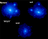Fig. 1.

Renderings of the projected density of DM in three similarly massive haloes selected from different cosmic web environments identified by CaCTus. Moving clockwise from the upper left, the haloes are selected from a filament, wall, and void environment, and have masses of M₂₀₀ = 8.3 × 10¹¹, 7.0 × 10¹¹, and 3.5 × 10¹¹ h⁻¹ M_⊙, respectively. The void halo presented here is one of the most massive found in that environment in the COLOR volume. After adjusting for the factor of two in halo mass, the most striking difference is the relative lack of massive subhaloes in the void host when compared to the other two.

Additionally, we introduce a synthetic sample called the equally weighted sample, constructed by reweighting the full population of host haloes in each cosmic web environment so that the effective contribution from each environment matches that of the environment with the smallest number of host haloes within each mass bin. This approach mitigates the sensitivity of our results to cosmic variance, which depends on the specific simulation volume we use. It also allows us to control for the bias introduced by using the cosmic mean sample, which consists of the combined set of all host haloes from walls, filaments, and voids in each mass bin. This tends to favour the richest environment, which across all mass bins is the filament environment. Throughout this paper, we characterise environmental trends by expressing subhalo properties as ratios relative to two distinct reference samples: (i) the cosmic mean, and (ii) the equally weighted sample. We denote the fractional deviation with respect to the cosmic mean as 𝒟 ≡ X/X_cm − 1, where X denotes a given subhalo statistic or property of interest. The deviation relative to the equally weighted sample is denoted as D ≡ X/X_eq − 1. These two measures, 𝒟 and D, allow us to probe global environmental effects while reducing sensitivity to the specific cosmic web makeup of the simulation box.

For the range of masses of our hosts, the halo mass function is a steep power-law. Thus, constructing host mass bins in decades of fixed width would skew the halo mass distribution towards the lower-mass end of the bin. To alleviate this problem, we group the host haloes into three bins in such a way that the resulting median masses in each bin are: ⟨M₂₀₀⟩=[10¹⁰,10¹¹,10¹²] h⁻¹ M_⊙. Table 1 shows the number density of the host haloes (the number of haloes in a given cosmic web environment divided by the volume occupied by that specific environment) in each mass bin across different environments. We provide the range of host halo masses spanned by each bin in each cosmic web environment in Table 2.

Table 1.

Number density of host haloes in each host mass bin in each cosmic web environment.

Table 2.

Host halo mass ranges of each mass bin, ⟨M₂₀₀⟩, for the halo sample in each cosmic web environment.

4.1. The subhalo mass function

Other works have established that the normalised abundance of haloes, or the halo mass function, may depend on environment (Cautun et al. 2014a; Alonso et al. 2015; Libeskind et al. 2018, H21). Specifically, H21 showed that within NEXUS+ environments, the fraction of haloes distributed among different cosmic web elements strongly depends on the halo virial mass. Cluster and group-mass haloes with M₂₀₀ ≳ 10¹³ h⁻¹ M_⊙ almost exclusively inhabit the densest parts of the cosmic web (i.e. the nodes). However, as the host mass decreases, less massive host haloes gradually dominate the host halo abundance in the other three environments (i.e. filaments, walls, and voids). The NEXUS+ segmentation hints at a trend towards an equipartition into those three environments at the smallest masses probed in H21, i.e. M₂₀₀ ≈ 10¹⁰ h⁻¹ M_⊙. The variation of halo abundance across the different cosmic web environments suggests that the averaged abundance of subhaloes should also be a function of the cosmic web environment. If the trends observed in halo abundance directly translate to subhalo abundance, then the abundance of the most massive subhaloes will be a strong function of the cosmic web environment of the host. If the most massive haloes (i.e. proto-subhaloes) live in filaments, hosts residing in voids and walls will have fewer large subhaloes. To quantify and check this, we first look at the subhalo mass function (SHMF).

In hierarchical structure formation models like CDM, it is convenient to express the subhalo mass in relation to the mass of its host. Thus, for each subhalo, we define the reduced subhalo mass, μ ≡ M_sub/M₂₀₀, and study the cumulative SHMF (cSHMF), N(≥μ), which is less susceptible to random Poissonian fluctuations than a differential SHMF. This will become useful, especially for low-mass hosts from the void and wall environments, where, as we show below, the hosts have few subhaloes.

In Fig. 2 we show the mean cSHMF, $\bar{N} (\geq μ)$ $\overline{N}(\geq\mu)$ , across each environment. Each panel corresponds to hosts binned by ⟨M₂₀₀⟩, and we differentiate the cSHMF into the following samples: hosts from the entire simulation volume (green triangles), those found in filaments (orange diamonds), walls (light blue circles), and voids (dark red squares). In addition, as mentioned earlier, as our unbiased reference point we plot the equally weighted sample (dark blue stars), drawn uniformly from all of those environments. In the middle subpanels, we show the fractional deviation, D(≥μ), of the cSHMFs for each environmental sample with respect to the equally weighted sample. By construction, an environmental sample with D = 0.2 contains 20% more subhaloes than the equally weighted sample, while D = −0.2 indicates a 20% deficit. To provide additional context, the lower subpanels in each figure show the fractional deviation of each environment relative to the cosmic mean, denoted D(≥μ). This serves as a cosmologically representative baseline and illustrates how the cSHMF in each environment differs from that of the entire halo population within the corresponding host mass bin. For the ⟨M₂₀₀⟩ = 10¹² h⁻¹ M_⊙ mass bin, we only find one host in the voids, thus, we ignore the void sample in that bin and focus only on the comparison between hosts in filament and wall environments. The error bars represent the standard error on the mean, estimated from 1000 bootstrap resamples. Finally, the two dashed lines illustrate a simple single power-law model for the cSHMF of the form $\bar{N} (\geq μ) \propto μ^{- s}$ $\overline{N}(\geq\mu)\propto \mu^{-s}$ , with the scale-free case of s = 1 shown by the black dashed line, and the COCO simulation best-fitting cases of s = 0.94, 0.93, and 0.92 for each respective host mass bin (Hellwing et al. 2016) with magenta lines. Comparing our data with the dashed lines, we find that a single power-law provides a good description of the cSHMF only up to a transition point μ ≲ μ_t. Beyond this scale, the cSHMF exhibits a significant exponential suppression relative to the power-law fit. For our three host halo mass bins, we estimate μ_t ∼ 0.03, 0.04, and 0.1, with the transition occurring at larger subhalo-to-host mass ratios for lower-mass hosts. This trend partially reflects the effects of simulation mass resolution: lower-mass host haloes can only reliably resolve relatively massive subhaloes, effectively shifting the onset of the cutoff to higher μ. In all cases, the deviation from the power-law exceeds 10% and lies beyond the 1σ bootstrap uncertainty, indicating a statistically robust departure from scale-free behaviour. This observation primarily applies to the cosmic mean and equally weighted sample. In all cases, the void cSHMFs appear to have a noticeably steeper slope than for the hosts in COCO and the COLOR equally weighted samples. The slope for the wall sample in the most massive bin is similarly steep. Across all environmental samples in all mass bins, the shape of the cSHMF in the regime of the most massive subhaloes, μ ≥ μ_t, significantly deviates from a uniform power-law.

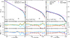Fig. 2.

Upper panels: mean cumulative subhalo mass functions for host haloes in three different mass bins, ⟨M₂₀₀⟩, shown as data points, sampled from different environments: cosmic mean (green triangles), filaments (yellow diamonds), walls (light blue circles), voids (dark red squares), and our synthetic equally weighted sample (dark blue stars). The error bars represent bootstrapped 1σ uncertainties. The solid lines with matching colours indicate the best fits to the exponential power-law model from Eq. (4). The grey shaded regions on the left of each panel indicate the subhalo resolution limit, μ_min. The two dashed lines illustrate the single power-law models for the scale-free case (black) and the best fit from the COCO simulations (magenta) of Hellwing et al. (2016). Middle panels: fractional deviation of each subhalo mass function with respect to the equally weighted sample, D. Lower panels: Fractional deviation with respect to the cosmic mean, 𝒟. The error bars in the ratio panels show uncertainties calculated through standard error propagation. We note the different ranges of the x-axes among the panels.

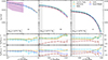Fig. 3.

Upper panels: fraction of the host halo mass in substructures. We show the same environmental samples as in Fig. 2 for the two mass bins where the μ ranges are above the resolution limits. As before, the error bars correspond to the bootstrapped 1σ errors. The grey shaded regions at the left of each panel show the subhalo resolution limit of the simulation. Middle panels: ratios of the substructure mass fraction in each environment with respect to the equally weighted sample, D. Lower panels: Ratios of the substructure mass fraction in each environment relative to the cosmic mean, 𝒟. The error bars in the ratio panel are estimated using standard error propagation. For comparison, we show the median and 60% scatter (dashed line and shaded region) from the MILLENNIUM II simulation (Gao et al. 2011).

The exponential decay of the subhalo abundance at large μ is not surprising. Major mergers, i.e. events that correspond to the accretion of a massive subhalo, are quite rare. This makes the capture of such subhaloes intrinsically stochastic and Poissonian (Fakhouri et al. 2010). Thus, a more realistic model for the cSHMF should take the form of an exponential power-law. To illustrate this, we consider the relationship proposed by Giocoli et al. (2010):

$\begin{matrix} \bar{N} (> μ) = a μ^{- s} exp (- β μ^{3}) . \end{matrix}$ $\begin{aligned} \overline{N}(>\mu ) = a\mu ^{-s}\exp (-\beta \mu ^3)\,. \end{aligned}$ (4)

Here a denotes the normalisation, s is a power-law exponent, and β is an exponential slope that determines the strength of the drop-off at high μ values. To determine the best-fitting values listed in Table 3, we fit the data only down to a specific μ_min value. For each host mass sample, μ_min represents the minimum converged subhalo mass, which we take to be equal to 100 × m_p. For COLOR, this sets our limiting subhalo mass to M_sub = 6.19 × 10⁸ h⁻¹ M_⊙. The grey shaded region represents values below the μ_min value for each mass bin.

Using the model from Eq. (4), we can now analyse our cSHMF in a more systematic way. In each cosmic web environment, the cSHMF is approximately universal within the μ regime where the SHMF closely follows a power-law, with only a weak dependence on the parent halo mass. This is in agreement with previous work (Diemand et al. 2004; Gao et al. 2004b; Van Den Bosch et al. 2005; Giocoli et al. 2008; Angulo et al. 2009; Chua et al. 2017; Gao et al. 2011; Jiang & Bosch 2016, H21). However, for μ ≥ μ_t the abundance of subhaloes decreases significantly and is described by a transition from a power-law to an exponential decay. The reduction of the cSHMF amplitude is especially prominent among subhaloes found in, on average, less massive haloes, which agrees with the previous results (Van Den Bosch et al. 2005; Reed et al. 2005).

Our results from Fig. 2 show that the cSHMF can differ substantially between hosts with the same mass located in different cosmic web environments. We find that haloes located in filaments contain, on average, the highest number of subhaloes, with 0.1 ≤ D(μ≥μ_t) < 0.2 as shown in the middle subpanels. In the most massive host bin, filament subhaloes contribute the largest share of subhaloes across this μ range. For the two lower-mass host bins, subhaloes in walls outnumber those in filaments just above μ_t. Filament subhaloes regain the largest contribution at the high-μ end. In comparison, perhaps unsurprisingly, hosts found in voids typically have the fewest subhaloes, with −0.05 ≤ D(μ≥μ_t) < −0.25. In all cases, the biggest differences between environments materialise for the large μ-values, i.e. in the regime of massive and rare subhaloes. Here, at μ ≳ μ_t, the relative differences between the mean cSHMF of the environmental samples and the equally weighted samples, D can be as large as 0.25. Thus, the abundance of massive subhaloes exhibits a strong dependence on the cosmic web environment of their host. This variation is captured by the best-fit values of the β-parameter, which we provide in Table 3.

Table 3.

Best-fitting β values and power-law slope s for cumulative subhalo mass functions.

In the low subhalo mass regime (μ ≲ μ_t), the differences between environments are more subtle but remain consistent with the trends discussed above. For the two most massive host halo bins, the cSHMF amplitude in filaments is elevated by approximately 5–20% relative to other environments. In the lowest host mass bin, however, walls exhibit the highest subhalo abundance, exceeding other environments by 5–12%. In contrast, voids consistently show a suppressed cSHMF that is lower by 5–25% across all mass bins. The cSHMFs also show that environmental effects typically become stronger with decreasing host mass. The lower subpanels illustrate how the cSHMF in each cosmic web environment deviates from the cosmic mean, as measured by 𝒟(≥μ). In the most massive host bin, filament subhaloes closely follow the cosmic mean, with 𝒟 ≈ 1. As the host mass decreases, the cSHMF in filaments is suppressed more strongly, with 𝒟 declining from −0.02 to −0.05. In contrast, the cSHMF in walls is enhanced as the host mass increases, with 𝒟 rising from 0.03 to 0.08. The abundance of subhaloes in void hosts remains consistently suppressed across all host mass bins, and we find the largest deficit, 𝒟 = −0.15, in massive subhaloes in the lowest-mass hosts.

Our results for the cSHMF show that the variation in subhalo abundance is both a function of the host mass and the cosmic web environment of the host. To reduce this complexity and obtain a more direct measure of the environmental effects, we look at the average expected total number of subhaloes above some mass threshold computed for hosts of different masses and cosmic web environments. We choose to count all subhaloes with μ ≥ 0.04 for a given host and compute the average per host mass bin and environment. We call this the subhalo richness because it corresponds to the mean expected number of subhaloes for a given host sample. We have collected the subhalo richness computed for all our host samples in Table 4. Subhalo richness exhibits a consistent host mass-dependent decline across environments. In the equally weighted sample, richness decreases by ∼14% from the 10¹² to 10¹¹ h⁻¹ M_⊙ bin, followed by a steeper 40% drop to the 10¹⁰ h⁻¹ M_⊙ bin. Filament and wall environments show similar trends, with initial reductions of 12% and 16%, respectively, between the two higher-mass bins, followed by more substantial decreases of 43% and 44% to the lowest-mass bin. In contrast to other environments, the void sample shows a more moderate reduction in subhalo richness, decreasing by 37% from the 10¹¹ to 10¹⁰ h⁻¹ M_⊙ bin.

Table 4.

Subhalo richness: Mean total number of subhaloes with μ ≥ 0.04 for all our host halo mass and environment samples.

The higher subhalo richness of hosts in filaments can be attributed to the dynamic environment that filaments provide for halo interactions and mergers. Haloes within filaments are situated in regions of higher matter density and experience stronger tidal forces, increasing the likelihood of substructure accretion through frequent gravitational encounters and mergers (Hahn et al. 2007b; Ganeshaiah Veena et al. 2018). In contrast, more underdense regions such as voids are characterised by slower structure formation, weaker tidal fields, and reduced merger activity. Consequently, haloes in voids tend to form later and accrete much less external material compared to their counterparts in denser environments (Gao et al. 2004a; Hahn et al. 2007b; Hellwing et al. 2021).

Another interesting quantity to investigate in the context of cosmic web effects is the fraction of the total mass of haloes contained in subhaloes,

$\begin{matrix} f_{sub} (\geq μ_{0}) = \int_{μ_{0}}^{1} μ \frac{d N}{d μ} . \end{matrix}$ $\begin{aligned} f_\mathrm{sub} (\ge \mu _0) = \int _{\mu _0}^{1} \mu \dfrac{\mathrm{d}N}{\mathrm{d}\mu }. \end{aligned}$ (5)

We can understand this as an effective measure of the halo granularity. Haloes with low fractions of mass locked in subhaloes should exhibit smoother density profiles, while in contrast large f_sub might indicate violent virialisation in progress and/or a significant number of recent mergers. Previous studies of high-resolution N-body simulations have established that typically the mass fraction locked in subhaloes (for μ ≳ 10⁻⁴ − 10⁻²) ranges from 5 to 20% of the host mass (Ghigna et al. 1998, 2000; de Lucia et al. 2004; Gao et al. 2004b, 2011; Contini et al. 2012).

In Fig. 3 we show the cumulative mass fraction in subhaloes as a function of the normalised subhalo mass, μ, for our five standard samples. The middle panels display the fractional deviation of the cumulative subhalo mass fraction, D(≥μ), for each environmental sample relative to the equally weighted baseline. The lower subpanels show the corresponding fractional deviation, 𝒟(≥μ), measured with respect to the cosmic mean sample. The variation across different cosmic web environments is not dramatic, with f_sub typically deviating by 2–20% from the equally weighted sample. For the majority of the samples, this observed effect is weak but statistically distinguishable within the 1σ bootstrap errors. There are a couple of interesting points of attention concerning the results shown in Fig. 3. First, we note that for the ⟨M₂₀₀⟩ = 10¹² h⁻¹ M_⊙ sample, our results agree well with what Gao et al. (2011) obtained for comparable host masses in the MILLENNIUM-II Simulation (shown with the dashed line and corresponding purple shaded region). For this host mass bin, the filament sample has higher mass fractions and the wall population exhibits lower values than the equally weighted sample. For the ⟨M₂₀₀⟩ = 10¹¹ h⁻¹ M_⊙ bin, we also see a bimodal effect on f_sub, but now where both filament and wall hosts have, on average, higher subhalo mass fractions, while only the void population displays lower values. The variation of f_sub with cosmic web environment is a sizeable effect which can potentially be important for strong lensing mass modelling studies. We leave a more thorough investigation into this matter for future studies.

4.2. The subhalo velocity function

So far, we have used the total subhalo mass, as identified by SUBFIND, to characterise the subhalo size. It is well known that, once subhaloes start orbiting within their hosts, they are subject to a strong and non-linear tidal mass stripping process. This makes the subhalo mass a less stable and sometimes even poorly defined quantity. Another way to characterise the size of a subhalo is to use the maximum of its circular orbit velocity, V_max. This quantity is less affected by the strong tidal processing of the subhalo because it depends on the total enclosed mass of the subhalo. Several studies have demonstrated that for many applications V_max is a robust halo size description (Ghigna et al. 1998, 2000; Muldrew et al. 2011; Knebe et al. 2011; Onions et al. 2012; Knebe et al. 2013; Cautun et al. 2014c).

Here, we use the subhalo velocity functions as another measure of subhalo size and abundance. The circular velocity, denoted as V_circ, is conventionally expressed as

$\begin{matrix} V_{circ} \equiv \sqrt{\frac{G M (< r)}{r}}, \end{matrix}$ $\begin{aligned} {V}_{\rm circ} \equiv \sqrt{\frac{GM( < r)}{r}}, \end{aligned}$ (6)

where M(< r) is the mass enclosed inside a sphere of radius, r, centred at the (sub)halo centre. Each subhalo has the maximum circular velocity, V_max, which represents the peak value of the circular velocity profile that is attained at a radius R_max. We use V_max as a stable measure of the abundance of the subhalo population.

In Fig. 4, we show the cumulative abundance of subhaloes (SHVF), $\bar{N} (> ν)$ $\overline{N}( > \nu)$ , as a function of ν = V_max/V₂₀₀, where V₂₀₀ is the circular velocity of the host halo at R₂₀₀. The subhaloes in bins of host masses (now with the corresponding ⟨V₂₀₀⟩ values) across different environments are presented in the same manner as described in Fig. 2. The solid red line presents the best-fit to the mean subhalo count in Milky Way-mass haloes within R₂₀₀ of the host from Cautun et al. (2014c). The middle subpanels show the fractional deviation of the SHVF, D(> ν), of each environmental sample with respect to the equally weighted sample. The lower subpanels present the fractional deviation compared to the cosmic mean sample, 𝒟(> ν). The qualitative behaviour with host samples and environments is similar to what we have seen in Fig. 2, albeit with some slight differences. As the host halo mass decreases, the dependence on the cosmic web environment increases. The environmental dependence of the abundance of subhaloes observed in Fig. 2 is confirmed in Fig. 4. However, while the SHMF shows a strong dependence on host halo mass, the SHVF exhibits a weaker but still noticeable dependence on host mass, consistent with findings from previous studies (Hellwing et al. 2016; Moliné et al. 2023). The fact that the environmental trends depicted both in SHMF and SHVF are in large qualitative agreement reassures us that the trends and effects we see here are real and robust down to the simulation resolution limit.

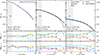Fig. 4.

Upper panels: mean cumulative distribution of subhaloes within R₂₀₀ as a function of ν = V_max/V₂₀₀ in the cosmic mean sample (green triangles), filaments (yellow diamonds), walls (light blue circles), voids (dark red squares), and the equally weighted sample (dark blue stars) for different host masses. The solid lines simply connect the data points, in contrast to Fig. 2 in which they represent fits to the data. In the legend, we provide the median V₂₀₀ for the given host halo mass bin. The solid red line in the figure depicts the best-fit function from Cautun et al. (2014c) for subhaloes within the radius R₂₀₀. The error bars represent the standard error on the mean, estimated from 1000 bootstrap resamples. Middle panels: Fractional deviation of $\bar{N} (> ν)$ $\overline{N}( > \nu)$ for each environment compared to the cumulative velocity function of an equally weighted sample, D. Lower panels: Deviation of $\bar{N} (> ν)$ $\overline{N}( > \nu)$ with respect to cosmic mean sample, 𝒟. The uncertainties shown in the ratio panels were computed through standard error propagation.

4.3. The V_max–R_max relation

In cosmologies that describe hierarchical structure formation, such as the CDM model, halo (and thus also subhalo) density profile concentrations correlate with specific formation times. This relationship arises because, during the hierarchical assembly of (sub)haloes, the innermost regions are the first to form. Material accreted later tends to have higher angular momentum, preventing it from settling in the central parts of the (sub)halo mass distribution. Consequently, the inner regions of (sub)halo density profiles are dynamically old, and the density achieved during assembly determines the (sub)halo concentration. As the Universe’s average background density decreases over time, older (sub)haloes typically exhibit higher central densities and concentrations (Wechsler et al. 2002; Gao et al. 2004b; Springel et al. 2008; Mao et al. 2015; Ludlow et al. 2016). Previous works (Bullock et al. 2001; Macció et al. 2007; Alonso et al. 2015,H21) have shown that halo concentration is dependent on the cosmic web environment. We want to check if this correlation is also exhibited by the host’s subhalo population. This corresponds to a picture where sub(haloes) forming in dense environments are likely to be more concentrated and form earlier (Bullock et al. 2001; Sheth & Tormen 2004; Avila-Reese et al. 2005; Harker et al. 2006; Wechsler et al. 2006; Maulbetsch et al. 2007; Ludlow et al. 2016; Chen et al. 2020).

To study the subhalo density profiles, we exploit the V_max–R_max relation. This can be readily used to study the internal kinematics and the associated density profiles of (sub)haloes (Springel et al. 2008; Hellwing et al. 2016). The relation stems from a strong correlation of (sub)halo internal kinematics with the internal mass distribution, allowing a reliable estimation of the steepness of the (sub)halo mass profile. Extra care should be taken here since the V_max can be affected by the gravitational softening length (ϵ). The general effect can lead to a reduction in the maximum circular velocities of subhaloes, particularly when the value of R_max is not significantly greater than ϵ. To address this, following Hellwing et al. (2016), we have applied the adequate correction proposed by Eq. (10) in Springel et al. (2008). This correction compensates approximately for the gravitational softening effect on V_max.

In Fig. 5, we show the mean V_max–R_max relation for our subhalo populations in various host and environmental samples. The error bars indicate the bootstrapped uncertainty on the means. To better highlight the trends, the middle subpanels show the fractional deviation, D, of the different samples taken with respect to the equally weighted one, while the lower subpanels display the same quantity but computed relative to the cosmic mean sample, 𝒟. The grey shaded region represents the area below the resolution limit of the COLOR box, V_max = 25 km s⁻¹ (see Hellwing et al. 2016 for more detailed analysis).

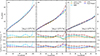Fig. 5.

The mean V_max–R_max relation of the subhaloes within R₂₀₀ for different host masses across different cosmic web environments. The error bars show the bootstrap errors on the mean. The grey shaded regions at the left of each panel show the subhalo resolution limit of the simulation. Upper panels: Solid lines with error bars represent subhaloes in voids (squares), walls (circles), filaments (diamonds), the cosmic mean sample (triangles), and the equally weighted sample (stars). Middle panels: Fractional deviation of the R_max values of each environment from that of the equally weighted sample, D. Lower panels: Relative divergence of R_max values compared to the full-volume sample, 𝒟. In the ratio panels, the error bars represent the uncertainty obtained via standard error propagation.

From Fig. 5 we draw three important findings. First, the mean R_max values for filament samples are lower than for other environments at fixed V_max. The middle subpanels in Fig. 5 show the fractional deviation of subhaloes in filaments with respect to the equally weighted sample, showing 1 − 8% suppression. This implies that, compared to walls and voids, subhaloes found in hosts in filaments have, on average, more concentrated density profiles. Conversely, the subhalo populations residing in haloes within voids have the highest mean R_max values, with showing a 1–8% enhancement. This suggests that subhaloes living in systems found in voids have, on average, less concentrated density profiles than the cosmic mean predicted for the whole CDM population.

Secondly, we find that the V_max–R_max relationship is affected more strongly by the environment as the host mass decreases. When examining the residuals in the 10¹¹ h⁻¹ M_⊙ bin (middle column of Fig. 5, middle subpanel), the largest differences between subhaloes in any given environment and the equally weighted sample ranges from 2 to 8%. However, this increases to approximately 3–9% in the 10¹⁰ h⁻¹ M_⊙ bin (middle subpanel of the right-hand column of Fig. 5).

The lower subpanels of Fig. 5 highlight how the R_max–V_max relation varies with environment relative to the average across all hosts within the same mass bin. In the highest-mass bin, filament subhaloes show mean R_max values that closely follow the cosmic mean. However, towards lower host masses, their R_max values fall increasingly further below the cosmic mean, with 𝒟 increasing in magnitude from about 2% to 5% below the mean. Wall subhaloes, by contrast, start ∼10% above the cosmic mean, then gradually approach the mean as host mass decreases. Subhaloes in voids remain consistently above the cosmic mean across all bins, with their largest deviation (𝒟 ∼ 0.08) appearing at the low-mass end.

One of the small-scale ΛCDM discrepancies, which was underscored by Boylan-Kolchin et al. (2011), is known as the too big to fail (TBTF) problem. It arises from a difference between the distribution of internal properties inferred for the most massive satellites of Milky Way mass hosts in the AQUARIUS simulation suite and the internal properties of the observed dwarf Milky Way satellites (Boylan-Kolchin et al. 2012). A similar assertion was made for the field dwarf galaxies discovered in the Local Group (Garrison-Kimmel et al. 2014). Many possible reasons have been proposed for the discrepancy, with some suggesting that processes connected to baryonic physics can lower the V_max values of subhaloes hosting dwarf galaxies, while others claim that assuming a lower virial mass of the Galactic DM halo (Sawala et al. 2013) could significantly alleviate the problem, given the strong correlation between the abundance of high V_max satellites and the host virial mass (Cautun et al. 2014b). The second feature we observe in Fig. 5 carries significant implications for the TBTF problem. Moving the Milky Way halo from a cosmic filament to a cosmic wall alleviates the TBTF problem by decreasing the number of high V_max satellites while increasing their R_max values. Our results also signify the importance of control over the cosmic environment when constructing theoretical predictions for subhalo kinematic and density distributions.

The third important observation concerns a trend associated with the mass of the parent halo. Specifically, at fixed V_max, subhaloes exhibit systematically lower mean R_max values when they are hosted by lower-mass haloes. To provide further detail, the environmental effects above V_max = 80 km s⁻¹ become noticeable within the 10¹² h⁻¹ M_⊙ mass bin. The difference becomes progressively pronounced, approximately ranging from 3 to 8% across all V_max values for bins within the range 10¹⁰ − 10¹¹ h⁻¹ M_⊙.

5. Summary and discussion

In this paper we analysed the impact of the cosmic web environment on the subhalo populations of host haloes at z = 0. To do this, we employed the CaCTus implementation of the NEXUS+ algorithm to segment the COLOR Gravity-only N-body simulation into four cosmic web environments (see Sections 2 and 3). We disentangled the competing effects of the host halo on the subhalo properties from those of the environment by dividing the subhalo populations into bins according to the masses of their hosts. We focused on host haloes with masses in the range ⟨M₂₀₀⟩ = 10¹⁰ to 10¹² h⁻¹ M_⊙. Our results extend previous studies that had already identified a strong relationship between DM halo properties and their respective locations within the cosmic web to smaller intrahalo scales.

Our main findings can be summarised as follows:

At fixed host mass, the abundance of subhaloes depends on the cosmic web environment of their hosts (Fig. 2). Host haloes with ⟨M₂₀₀⟩ = 10¹⁰ h⁻¹ M_⊙ in walls have subhaloes that are as much as two times more massive than hosts with the same mass in voids. At subhalo masses below μ_t the abundance of subhaloes in wall haloes is only 25% greater than in void haloes. The size of these differences decreases as the host halo mass is increased.
The measure of the halo granularity, the mass fraction in subhaloes, f_sub, shows a sizeable variation with the cosmic web (Fig. 3). Here, typically filament hosts tend to be more granular, with 2–15% more mass in subhaloes than void hosts. Void hosts, on the other hand, have 5–15% less mass in subhaloes and are characterised by a smoother density distribution. Generally, lower-mass hosts show a stronger dependence on the cosmic web.
The absolute difference in velocity functions between different environments is smaller than the difference in mass functions (Fig. 4). Subhaloes in filaments have 5–15% higher subhalo abundance in the velocity function, while subhaloes in voids have 5–25% lower abundance relative to the cosmic mean. This is because subhaloes with similar masses can have very different V_max.
The relative differences between the velocity functions in various environments are generally smaller than what we observe for mass functions. Generally, we start to observe a greater than 10% environmental difference in the velocity function above 0.5 V₂₀₀ for the most massive host bin. For lower-mass hosts, the differences are seen for a larger range of subhalo ν values.
Subhaloes in filaments are most concentrated, and those in voids are least concentrated (Fig. 5). This corresponds to an approximate 5 to 9% suppression in concentration for void subhaloes relative to filament subhaloes across all host mass bins, although in the 10¹² h⁻¹ M_⊙ bin it is largely absent below V_max = 80 km s⁻¹.
The characteristic density profile also displays a dependence on the parent halo mass by showing a reduction of R_max value as the host halo mass decreases.

Our results indicate that the abundance and internal properties of subhalo populations depend on the cosmic web environment of their host. The influence of this environment becomes stronger as the host halo mass decreases below the Milky Way mass scale. Studies that do not account for this intrinsic link between the properties of subhalo populations and the large-scale environment may be affected by systematic uncertainties that bias their results.

In this paper we analysed the SHMF as a function of μ = M_sub/M₂₀₀ in different cosmic web environments. The SHMF exhibits a dependence on the cosmic web environment in which they are located. The environmental effect on the mass function becomes more noticeable with decreasing host halo mass. This is consistent with the same trend observed in the host halo mass function, as previously demonstrated in H21. Our results specifically revealed the relative differences in the SHMFs across different environments exceeding 10% at lower host mass ranges. Subhaloes in voids exhibited consistently lower numbers compared to those in filaments and walls. Interestingly, the normalisation and the power-law slope of the mass functions displayed a similar pattern across all environments and with a slight dependence on host masses. However, the exponential slope, β, influencing the drop-off at the higher-mass end, shows a dependence on the cosmic web environment and the parent halo mass. Furthermore, in agreement with previous studies (Gao et al. 2004a; Giocoli et al. 2008; Ishiyama et al. 2013), our findings demonstrate a dependency of the SHMF on the host halo mass.

The fraction of the host mass contained in subhaloes, f_sub, is highest in filament environments, indicating that filament hosts are more substructure-rich, or more granular, than their counterparts in other cosmic web environments. This supports the idea that filaments promote subhalo accretion and survival through enhanced merger activity (Bond et al. 1996; Colberg et al. 2005; Ma et al. 2025). By contrast, haloes in voids tend to exhibit smoother density profiles, reflecting their more isolated and quiescent environments and assembly histories. These findings are consistent with the results of Hellwing et al. (2021), who showed that halo accretion histories are affected strongly by their cosmic web environment, with filament haloes undergoing more frequent mergers.

In addition, we analysed the subhalo velocity function to investigate an alternative perspective on the abundance of subhaloes within the cosmic web. It shows a similar dependence on the cosmic web environment such as the mass function. The environmental effect on the velocity functions becomes more pronounced with decreasing parent halo mass. In a manner similar to the mass function, subhaloes hosted by haloes within filaments exhibit a higher population count compared to those in walls and voids in massive host haloes. However, a shift occurs in the case of low-mass hosts, where subhaloes hosted by haloes located in walls show a larger population than those in other environments, and the relative difference is 5–10% higher than in the mass function.

Furthermore, we investigated the V_max − R_max relation of subhaloes, which characterises the concentration or characteristic density of subhaloes based on their maximum circular velocity and radius. This comprehensive analysis revealed different density profiles among subhaloes hosted by haloes residing within filaments, walls, and voids. Particularly, subhaloes within filaments and walls exhibited, on average, more concentrated density profiles compared to those inhabiting voids. Moreover, we found that this relation is affected by the mass of their host haloes. Interestingly, a discernible trend emerged: subhalo characteristics displayed lower dependence on cosmic web environments within higher-mass host haloes. However, a moresubstantial environmental impact became apparent with decreasing host halo mass. Notably, subhaloes hosted within filaments exhibited significantly more concentrated density profiles, particularly within lower-mass parent haloes, compared to those within massive hosts. Conversely, subhaloes in voids show on average less concentrated density profiles than in other environments. Another noteworthy feature of our results is that subhaloes tend to display lower R_max values when associated with low-mass hosts, especially in contrast to subhaloes hosted by massive haloes. This finding suggests that the characteristic density of subhaloes is not exclusively determined by their environmental location but is notably influenced by the mass of the parent halo.

It is well established that the overall properties of a subhalo, such as its mass measured at the virial radius, can be determined reliably with as few as 50 − 100 simulation particles (e.g. Springel et al. 2008; Onions et al. 2012; van den Bosch & Jiang 2016; Ludlow et al. 2019). However, such low particle counts are generally insufficient to accurately characterise the internal properties of subhaloes, such as their circular velocity profiles or concentrations. Studies have shown that subhaloes resolved with fewer than 3000 particles can exhibit significant deviations in their internal properties from converged results (Errani & Navarro 2021). Additionally, the choice of softening length and simulation time-step can further elevate the required resolution limit (van den Bosch & Ogiya 2018). The COLOR subhalo populations are not immune to numerical resolution effects, which can introduce both random and systematic biases. However, in our analysis, we mitigate these biases by studying the averaged internal properties of subhaloes within fixed mass and V_max bins. Importantly, we carefully compare subhalo populations using equally weighted samples constructed from hosts within the same bin. This approach largely eliminates systematic uncertainties arising from finite resolution effects when interpreting our results. While numerical instabilities can introduce additional random scatter in the properties of subhaloes, they do not strongly affect the intrinsic differences in the average properties caused by the cosmic web environment. As a result, our findings remain robust down to the resolution limits of the simulations in the mass ranges we consider.

An important consideration in our analysis is the relatively small volume of the COLOR simulation (∼100³ Mpc³), which may introduce some level of cosmic variance in the distribution of cosmic web environments. However, comparisons of volume and mass-filling fractions between COLOR and the larger Millennium simulation (Springel et al. 2005; Boylan-Kolchin et al. 2009), as reported by Hellwing et al. (2021), indicate that such effects are unlikely to significantly impact our results. Although some variation is expected due to the finite box size, our focus on relative differences across environments-rather than absolute values-helps preserve the robustness of our conclusions. Moreover, the use of an equally weighted sampling scheme, which enforces uniform representation across environments, further mitigates biases that could arise from the overabundance of structures like filaments in the full-volume distribution. A more detailed assessment of cosmic variance, particularly in underdense environments such as voids, is deferred to future work.

Addressing the ‘small-scale challenges to the ΛCDM paradigm’ requires a comprehensive approach that accounts for the influence of the cosmic environment. This research is the next step towards understanding the detailed influence of large-scale structures on the distribution and formation mechanisms of satellite galaxies. We will explore the dependence of the properties of subhaloes on the cosmic web environment in alternative DM scenarios and at higher redshifts in future work.

¹

CaCTus is being prepared for public release. At the time of writing it is not yet publicly available.

Acknowledgments

We thank the anonymous referee for insightful comments and questions that have helped improve the paper. We would like to thank Marius Cautun for constructive communication and comments on the implementation of NEXUS+ algorithm. Mariana Jaber, Rob Crain, Adi Nusser, Rien van de Weygaert, and Mike Hudson are acknowledged for enlightening discussions we had at various stages of this project. This work is supported via the research projects ‘COLAB’ and ‘LUSTRE’ funded by the National Science Center, Poland, under agreement number UMO-2020/39/B/ST9/03494 and UMO-2018/31/G/ST9/03388. MB is also supported by the Polish National Science Center through grants no. 2020/38/E/ST9/00395 and 2018/30/E/ST9/00698.

References

Adler, R. J. 1981, The Geometry of Random Fields (New York: Wiley) [Google Scholar]
Alonso, D., Eardley, E., & Peacock, J. A. 2015, MNRAS, 447, 2683 [Google Scholar]
Angulo, R. E., Lacey, C. G., Baugh, C. M., & Frenk, C. S. 2009, MNRAS, 399, 983 [CrossRef] [Google Scholar]
Aragón-Calvo, M. A., Jones, B. J. T., van de Weygaert, R., & van der Hulst, J. M. 2007a, A&A, 474, 315 [NASA ADS] [CrossRef] [EDP Sciences] [Google Scholar]
Aragón-Calvo, M. A., van de Weygaert, R., Jones, B. J. T., & van der Hulst, J. M. 2007b, ApJ, 655, L5 [Google Scholar]
Aragón-Calvo, M. A., Platen, E., van de Weygaert, R., & Szalay, A. S. 2010, ApJ, 723, 364 [Google Scholar]
Aragon Calvo, M. A., Neyrinck, M. C., & Silk, J. 2019, Open J. Astrophys., 2, 7 [CrossRef] [Google Scholar]
Avila-Reese, V., Colín, P., Gottlöber, S., Firmani, C., & Maulbetsch, C. 2005, ApJ, 634, 51 [Google Scholar]
Bardeen, J. M., Bond, J. R., Kaiser, N., & Szalay, A. S. 1986, ApJ, 304, 15 [Google Scholar]
Benítez-Llambay, A., Navarro, J. F., Abadi, M. G., et al. 2013, ApJ, 763, L41 [Google Scholar]
Blumenthal, G. R., Faber, S. M., Primack, J. R., & Rees, M. J. 1984, Nature, 311, 517 [Google Scholar]
Bond, J. R., Kofman, L., & Pogosyan, D. 1996, Nature, 380, 603 [NASA ADS] [CrossRef] [Google Scholar]
Bond, N. A., Strauss, M. A., & Cen, R. 2010, MNRAS, 409, 156 [NASA ADS] [CrossRef] [Google Scholar]
Bose, S., Hellwing, W. A., Frenk, C. S., et al. 2016, MNRAS, 455, 318 [NASA ADS] [CrossRef] [Google Scholar]
Boylan-Kolchin, M., Springel, V., White, S. D. M., Jenkins, A., & Lemson, G. 2009, MNRAS, 398, 1150 [Google Scholar]
Boylan-Kolchin, M., Bullock, J. S., & Kaplinghat, M. 2011, MNRAS, 415, L40 [NASA ADS] [CrossRef] [Google Scholar]
Boylan-Kolchin, M., Bullock, J. S., & Kaplinghat, M. 2012, MNRAS, 422, 1203 [NASA ADS] [CrossRef] [Google Scholar]
Bullock, J. S., Kolatt, T. S., Sigad, Y., et al. 2001, MNRAS, 321, 559 [Google Scholar]
Cautun, M., van de Weygaert, R., & Jones, B. J. T. 2013, MNRAS, 429, 1286 [NASA ADS] [CrossRef] [Google Scholar]
Cautun, M., van de Weygaert, R., Jones, B. J. T., & Frenk, C. S. 2014a, MNRAS, 441, 2923 [Google Scholar]
Cautun, M., Frenk, C. S., van de Weygaert, R., Hellwing, W. A., & Jones, B. J. T. 2014b, MNRAS, 445, 2049 [NASA ADS] [CrossRef] [Google Scholar]
Cautun, M., Hellwing, W. A., van de Weygaert, R., et al. 2014c, MNRAS, 445, 1820 [Google Scholar]
Cautun, M., Bose, S., Frenk, C. S., et al. 2015, MNRAS, 452, 3838 [NASA ADS] [CrossRef] [Google Scholar]
Chen, Y., Mo, H. J., Li, C., et al. 2020, ApJ, 899, 81 [NASA ADS] [CrossRef] [Google Scholar]
Chua, K. T. E., Pillepich, A., Rodriguez-Gomez, V., et al. 2017, MNRAS, 472, 4343 [NASA ADS] [CrossRef] [Google Scholar]
Colberg, J. M., Krughoff, K. S., & Connolly, A. J. 2005, MNRAS, 359, 272 [NASA ADS] [CrossRef] [Google Scholar]
Colless, M., Peterson, B. A., Jackson, C., et al. 2003, ArXiv e-prints [arXiv:astro-ph/0306581] [Google Scholar]
Contini, E., De Lucia, G., & Borgani, S. 2012, MNRAS, 420, 2978 [NASA ADS] [CrossRef] [Google Scholar]
Danovich, M., Dekel, A., Hahn, O., Ceverino, D., & Primack, J. 2015, MNRAS, 449, 2087 [Google Scholar]
Darvish, B., Mobasher, B., Martin, D. C., et al. 2017, ApJ, 837, 16 [Google Scholar]
Davis, M., Efstathiou, G., Frenk, C. S., & White, S. D. M. 1985, ApJ, 292, 371 [Google Scholar]
de Lapparent, V., Geller, M. J., & Huchra, J. P. 1986, ApJ, 302, L1 [Google Scholar]
de Lucia, G., Kauffmann, G., Springel, V., et al. 2004, MNRAS, 348, 333 [NASA ADS] [CrossRef] [Google Scholar]
Deason, A. J., Bose, S., Fattahi, A., et al. 2022, MNRAS, 511, 4044 [NASA ADS] [CrossRef] [Google Scholar]
Diemand, J., Moore, B., & Stadel, J. 2004, MNRAS, 353, 624 [NASA ADS] [CrossRef] [Google Scholar]
Dome, T., Fialkov, A., Sartorio, N., & Mocz, P. 2023, MNRAS, 525, 348 [NASA ADS] [CrossRef] [Google Scholar]
Doroshkevich, A. G. 1970, Astrophysics, 6, 320 [Google Scholar]
Dressler, A. 1980, ApJ, 236, 351 [Google Scholar]
Dupuy, A., Libeskind, N. I., Hoffman, Y., et al. 2022, MNRAS, 516, 4576 [NASA ADS] [CrossRef] [Google Scholar]
Enzi, W., Murgia, R., Newton, O., et al. 2021, MNRAS, 506, 5848 [NASA ADS] [CrossRef] [Google Scholar]
Errani, R., & Navarro, J. F. 2021, MNRAS, 505, 18 [NASA ADS] [CrossRef] [Google Scholar]
Fakhouri, O., Ma, C.-P., & Boylan-Kolchin, M. 2010, MNRAS, 406, 2267 [Google Scholar]
Feldbrugge, J., van de Weygaert, R., Hidding, J., & Feldbrugge, J. 2018, JCAP, 2018, 027 [Google Scholar]
Forero-Romero, J. E., Hoffman, Y., Gottlöber, S., Klypin, A., & Yepes, G. 2009, MNRAS, 396, 1815 [Google Scholar]
Forero-Romero, J. E., Contreras, S., & Padilla, N. 2014, MNRAS, 443, 1090 [NASA ADS] [CrossRef] [Google Scholar]
Frenk, C. S., & White, S. D. M. 2012, Annalen der Physik, 524, 507 [NASA ADS] [CrossRef] [Google Scholar]
Gámez-Marín, M., Santos-Santos, I., Domínguez-Tenreiro, R., et al. 2024, ApJ, 965, 154 [CrossRef] [Google Scholar]
Ganeshaiah Veena, P., Cautun, M., van de Weygaert, R., et al. 2018, MNRAS, 481, 414 [NASA ADS] [CrossRef] [Google Scholar]
Ganeshaiah Veena, P., Cautun, M., Tempel, E., van de Weygaert, R., & Frenk, C. S. 2019, MNRAS, 487, 1607 [NASA ADS] [CrossRef] [Google Scholar]
Ganeshaiah Veena, P., Cautun, M., van de Weygaert, R., Tempel, E., & Frenk, C. S. 2021, MNRAS, 503, 2280 [NASA ADS] [CrossRef] [Google Scholar]
Gao, L., Lucia, G. D., White, S. D., & Jenkins, A. 2004a, MNRAS, 352, L1 [NASA ADS] [CrossRef] [Google Scholar]
Gao, L., White, S. D. M., Jenkins, A., Stoehr, F., & Springel, V. 2004b, MNRAS, 355, 819 [Google Scholar]
Gao, L., Springel, V., & White, S. D. M. 2005, MNRAS, 363, L66 [NASA ADS] [CrossRef] [Google Scholar]
Gao, L., Frenk, C. S., Boylan-Kolchin, M., et al. 2011, MNRAS, 410, 2309 [Google Scholar]
Gao, L., Navarro, J. F., Frenk, C. S., et al. 2012, MNRAS, 425, 2169 [NASA ADS] [CrossRef] [Google Scholar]
Garrison-Kimmel, S., Boylan-Kolchin, M., Bullock, J. S., & Kirby, E. N. 2014, MNRAS, 444, 222 [NASA ADS] [CrossRef] [Google Scholar]
Ghigna, S., Moore, B., Governato, F., et al. 1998, MNRAS, 300, 146 [NASA ADS] [CrossRef] [Google Scholar]
Ghigna, S., Moore, B., Governato, F., et al. 2000, ApJ, 544, 616 [NASA ADS] [CrossRef] [Google Scholar]
Gillet, N., Ocvirk, P., Aubert, D., et al. 2015, ApJ, 800, 34 [NASA ADS] [CrossRef] [Google Scholar]
Giocoli, C., Tormen, G., & Van Den Bosch, F. C. 2008, MNRAS, 386, 2135 [NASA ADS] [CrossRef] [Google Scholar]
Giocoli, C., Tormen, G., Sheth, R. K., & van den Bosch, F. C. 2010, MNRAS, 404, 502 [NASA ADS] [Google Scholar]
González, R. E., & Padilla, N. D. 2016, ApJ, 829, 58 [Google Scholar]
Guo, Q., Tempel, E., & Libeskind, N. I. 2015, ApJ, 800, 112 [Google Scholar]
Hahn, O., Carollo, C. M., Porciani, C., & Dekel, A. 2007a, MNRAS, 381, 41 [NASA ADS] [CrossRef] [Google Scholar]
Hahn, O., Porciani, C., Carollo, C. M., & Dekel, A. 2007b, MNRAS, 375, 489 [NASA ADS] [CrossRef] [Google Scholar]
Hammer, F., Yang, Y., Fouquet, S., et al. 2013, MNRAS, 431, 3543 [NASA ADS] [CrossRef] [Google Scholar]
Han, J., Jing, Y. P., Wang, H., & Wang, W. 2012, MNRAS, 427, 2437 [NASA ADS] [CrossRef] [Google Scholar]
Han, J., Cole, S., Frenk, C. S., & Jing, Y. 2016, MNRAS, 457, 1208 [NASA ADS] [CrossRef] [Google Scholar]
Harker, G., Cole, S., Helly, J., Frenk, C., & Jenkins, A. 2006, MNRAS, 367, 1039 [NASA ADS] [CrossRef] [Google Scholar]
Hellwing, W. A., Frenk, C. S., Cautun, M., et al. 2016, MNRAS, 457, 3492 [NASA ADS] [CrossRef] [Google Scholar]
Hellwing, W. A., Cautun, M., van de Weygaert, R., & Jones, B. T. 2021, Phys. Rev. D, 103, 063517 [NASA ADS] [CrossRef] [Google Scholar]
Hoffman, Y., Metuki, O., Yepes, G., et al. 2012, MNRAS, 425, 2049 [Google Scholar]
Ibata, R. A., Lewis, G. F., Conn, A. R., et al. 2013, Nature, 493, 62 [NASA ADS] [CrossRef] [Google Scholar]
Ishiyama, T., Rieder, S., Makino, J., et al. 2013, ApJ, 767, 146 [NASA ADS] [CrossRef] [Google Scholar]
Jiang, F., & Bosch, F. C. V. D. 2016, MNRAS, 458, 2848 [NASA ADS] [CrossRef] [Google Scholar]
Klypin, A., Kravtsov, A. V., Valenzuela, O., & Prada, F. 1999, ApJ, 522, 82 [Google Scholar]
Knebe, A., Knollmann, S. R., Muldrew, S. I., et al. 2011, MNRAS, 415, 2293 [Google Scholar]
Knebe, A., Pearce, F. R., Lux, H., et al. 2013, MNRAS, 435, 1618 [NASA ADS] [CrossRef] [Google Scholar]
Komatsu, E., Smith, K. M., Dunkley, J., et al. 2011, ApJS, 192, 18 [Google Scholar]
Libeskind, N. I., Frenk, C. S., Cole, S., et al. 2005, MNRAS, 363, 146 [NASA ADS] [CrossRef] [Google Scholar]
Libeskind, N. I., Hoffman, Y., Knebe, A., et al. 2012, MNRAS, 421, L137 [NASA ADS] [CrossRef] [Google Scholar]
Libeskind, N. I., Hoffman, Y., Tully, R. B., et al. 2015, MNRAS, 452, 1052 [NASA ADS] [CrossRef] [Google Scholar]
Libeskind, N. I., van de Weygaert, R., Cautun, M., et al. 2018, MNRAS, 473, 1195 [NASA ADS] [CrossRef] [Google Scholar]
Lovell, M. R., Cautun, M., Frenk, C. S., Hellwing, W. A., & Newton, O. 2021, MNRAS, 507, 4826 [NASA ADS] [CrossRef] [Google Scholar]
Ludlow, A. D., Bose, S., Angulo, R. E., et al. 2016, MNRAS, 460, 1214 [Google Scholar]
Ludlow, A. D., Schaye, J., & Bower, R. 2019, MNRAS, 488, 3663 [Google Scholar]
Ma, W., Guo, H., & Jones, M. G. 2025, A&A, 695, A5 [NASA ADS] [CrossRef] [EDP Sciences] [Google Scholar]
Macció, A. V., Dutton, A. A., Van Den Bosch, F. C., et al. 2007, MNRAS, 378, 55 [NASA ADS] [CrossRef] [Google Scholar]
Malavasi, N., Langer, M., Aghanim, N., Galárraga-Espinosa, D., & Gouin, C. 2022, A&A, 658, A113 [NASA ADS] [CrossRef] [EDP Sciences] [Google Scholar]
Mao, Y.-Y., Williamson, M., & Wechsler, R. H. 2015, ApJ, 810, 21 [NASA ADS] [CrossRef] [Google Scholar]
Maulbetsch, C., Avila-Reese, V., Colín, P., et al. 2007, ApJ, 654, 53 [NASA ADS] [CrossRef] [Google Scholar]
Metuki, O., Libeskind, N. I., Hoffman, Y., Crain, R. A., & Theuns, T. 2015, MNRAS, 446, 1458 [NASA ADS] [CrossRef] [Google Scholar]
Metuki, O., Libeskind, N. I., & Hoffman, Y. 2016, MNRAS, 460 [Google Scholar]
Miraghaei, H. 2020, AJ, 160, 227 [Google Scholar]
Moliné, Á., Sánchez-Conde, M. A., Aguirre-Santaella, A., et al. 2023, MNRAS, 518, 157 [Google Scholar]
Muldrew, S. I., Pearce, F. R., & Power, C. 2011, MNRAS, 410, 2617 [Google Scholar]
Müller, O., Pawlowski, M. S., Jerjen, H., & Lelli, F. 2018, Science, 359, 534 [CrossRef] [Google Scholar]
Newton, O., Leo, M., Cautun, M., et al. 2021, JCAP, 2021, 062 [CrossRef] [Google Scholar]
Newton, O., Lovell, M. R., Frenk, C. S., et al. 2024, ArXiv e-prints [arXiv:2408.16042] [Google Scholar]
Nurmi, P., Heinämäki, P., Holopainen, J., et al. 2007, in Galaxy Evolution across the Hubble Time, eds. F. Combes, & J. Palouš, 235, 127 [Google Scholar]
Onions, J., Knebe, A., Pearce, F. R., et al. 2012, MNRAS, 423, 1200 [Google Scholar]
Patiri, S. G., Cuesta, A. J., Prada, F., Betancort-Rijo, J., & Klypin, A. 2006, ApJ, 652, L75 [NASA ADS] [CrossRef] [Google Scholar]
Pawlowski, M. S., Kroupa, P., Angus, G., et al. 2012a, MNRAS, 424, 80 [NASA ADS] [CrossRef] [Google Scholar]
Pawlowski, M. S., Pflamm-Altenburg, J., & Kroupa, P. 2012b, MNRAS, 423, 1109 [NASA ADS] [CrossRef] [Google Scholar]
Peebles, P. J. E. 1980, The Large-scale Structure of the Universe (Princeton: Princeton University Press) [Google Scholar]
Pomarède, D., Hoffman, Y., Courtois, H. M., & Tully, R. B. 2017, ApJ, 845, 55 [Google Scholar]
Reed, D., Governato, F., Quinn, T., et al. 2005, MNRAS, 359, 237 [Google Scholar]
Rey, M. P., Pontzen, A., & Saintonge, A. 2019, MNRAS, 485, 1906 [Google Scholar]
Sawala, T., Frenk, C. S., Crain, R. A., et al. 2013, MNRAS, 431, 1366 [NASA ADS] [CrossRef] [Google Scholar]
Shandarin, S. F., & Zeldovich, Y. B. 1989, Rev. Mod. Phys., 61, 185 [NASA ADS] [CrossRef] [Google Scholar]
Sheth, R. K., & Tormen, G. 2004, MNRAS, 350, 1385 [NASA ADS] [CrossRef] [Google Scholar]
Sousbie, T. 2011, MNRAS, 414, 350 [NASA ADS] [CrossRef] [Google Scholar]
Springel, V., White, S. D. M., Tormen, G., & Kauffmann, G. 2001, MNRAS, 328, 726 [Google Scholar]
Springel, V., White, S. D. M., Jenkins, A., et al. 2005, Nature, 435, 629 [Google Scholar]
Springel, V., Wang, J., Vogelsberger, M., et al. 2008, MNRAS, 391, 1685 [Google Scholar]
Stoehr, F., White, S. D. M., Tormen, G., & Springel, V. 2002, MNRAS, 335, L84 [Google Scholar]
Tegmark, M., Blanton, M. R., Strauss, M. A., et al. 2004, ApJ, 606, 702 [Google Scholar]
Tempel, E., Guo, Q., Kipper, R., & Libeskind, N. I. 2015, MNRAS, 450, 2727 [NASA ADS] [CrossRef] [Google Scholar]
van de Weygaert, R., & Platen, E. 2011, Int. J. Mod. Phys. Conf. Ser., 1, 41 [NASA ADS] [CrossRef] [Google Scholar]
van den Bosch, F. C., & Jiang, F. 2016, MNRAS, 458, 2870 [Google Scholar]
van den Bosch, F. C., & Ogiya, G. 2018, MNRAS, 475, 4066 [NASA ADS] [CrossRef] [Google Scholar]
Van Den Bosch, F. C., Tormen, G., & Giocoli, C. 2005, MNRAS, 359, 1029 [NASA ADS] [CrossRef] [Google Scholar]
Wang, C.-W., Cooper, A. P., Bose, S., Frenk, C. S., & Hellwing, W. A. 2023, ApJ, 958, 166 [Google Scholar]
Wang, H. Y., Mo, H. J., & Jing, Y. P. 2007, MNRAS, 375, 633 [NASA ADS] [CrossRef] [Google Scholar]
Wang, L., Gonzalez-Perez, V., Xie, L., et al. 2017, MNRAS, 468, 4579 [Google Scholar]
Wang, P., Libeskind, N. I., Tempel, E., et al. 2020, ApJ, 900, 129 [NASA ADS] [CrossRef] [Google Scholar]
Wechsler, R. H., Bullock, J. S., Primack, J. R., Kravtsov, A. V., & Dekel, A. 2002, ApJ, 568, 52 [NASA ADS] [CrossRef] [Google Scholar]
Wechsler, R. H., Zentner, A. R., Bullock, J. S., Kravtsov, A. V., & Allgood, B. 2006, ApJ, 652, 71 [NASA ADS] [CrossRef] [Google Scholar]
White, S. D. M., & Frenk, C. S. 1991, ApJ, 379, 52 [Google Scholar]
White, S. D. M., & Rees, M. J. 1978, MNRAS, 183, 341 [Google Scholar]
Xu, W., Guo, Q., Zheng, H., et al. 2020, MNRAS, 498, 1839 [Google Scholar]
Zel’dovich, Y. B. 1970, A&A, 5, 84 [NASA ADS] [Google Scholar]
Zhang, Y., Yang, X., & Guo, H. 2021, MNRAS, 507, 5320 [Google Scholar]

All Tables

Table 1.

Number density of host haloes in each host mass bin in each cosmic web environment.

In the text

Table 2.

Host halo mass ranges of each mass bin, ⟨M₂₀₀⟩, for the halo sample in each cosmic web environment.

In the text

Table 3.

Best-fitting β values and power-law slope s for cumulative subhalo mass functions.

In the text

Table 4.

Subhalo richness: Mean total number of subhaloes with μ ≥ 0.04 for all our host halo mass and environment samples.

In the text

All Figures

Fig. 1.

Renderings of the projected density of DM in three similarly massive haloes selected from different cosmic web environments identified by CaCTus. Moving clockwise from the upper left, the haloes are selected from a filament, wall, and void environment, and have masses of M₂₀₀ = 8.3 × 10¹¹, 7.0 × 10¹¹, and 3.5 × 10¹¹ h⁻¹ M_⊙, respectively. The void halo presented here is one of the most massive found in that environment in the COLOR volume. After adjusting for the factor of two in halo mass, the most striking difference is the relative lack of massive subhaloes in the void host when compared to the other two.

In the text

Fig. 2.

Upper panels: mean cumulative subhalo mass functions for host haloes in three different mass bins, ⟨M₂₀₀⟩, shown as data points, sampled from different environments: cosmic mean (green triangles), filaments (yellow diamonds), walls (light blue circles), voids (dark red squares), and our synthetic equally weighted sample (dark blue stars). The error bars represent bootstrapped 1σ uncertainties. The solid lines with matching colours indicate the best fits to the exponential power-law model from Eq. (4). The grey shaded regions on the left of each panel indicate the subhalo resolution limit, μ_min. The two dashed lines illustrate the single power-law models for the scale-free case (black) and the best fit from the COCO simulations (magenta) of Hellwing et al. (2016). Middle panels: fractional deviation of each subhalo mass function with respect to the equally weighted sample, D. Lower panels: Fractional deviation with respect to the cosmic mean, 𝒟. The error bars in the ratio panels show uncertainties calculated through standard error propagation. We note the different ranges of the x-axes among the panels.

In the text

Fig. 3.

Upper panels: fraction of the host halo mass in substructures. We show the same environmental samples as in Fig. 2 for the two mass bins where the μ ranges are above the resolution limits. As before, the error bars correspond to the bootstrapped 1σ errors. The grey shaded regions at the left of each panel show the subhalo resolution limit of the simulation. Middle panels: ratios of the substructure mass fraction in each environment with respect to the equally weighted sample, D. Lower panels: Ratios of the substructure mass fraction in each environment relative to the cosmic mean, 𝒟. The error bars in the ratio panel are estimated using standard error propagation. For comparison, we show the median and 60% scatter (dashed line and shaded region) from the MILLENNIUM II simulation (Gao et al. 2011).

In the text

Fig. 4.

Upper panels: mean cumulative distribution of subhaloes within R₂₀₀ as a function of ν = V_max/V₂₀₀ in the cosmic mean sample (green triangles), filaments (yellow diamonds), walls (light blue circles), voids (dark red squares), and the equally weighted sample (dark blue stars) for different host masses. The solid lines simply connect the data points, in contrast to Fig. 2 in which they represent fits to the data. In the legend, we provide the median V₂₀₀ for the given host halo mass bin. The solid red line in the figure depicts the best-fit function from Cautun et al. (2014c) for subhaloes within the radius R₂₀₀. The error bars represent the standard error on the mean, estimated from 1000 bootstrap resamples. Middle panels: Fractional deviation of $\bar{N} (> ν)$ $\overline{N}( > \nu)$ for each environment compared to the cumulative velocity function of an equally weighted sample, D. Lower panels: Deviation of $\bar{N} (> ν)$ $\overline{N}( > \nu)$ with respect to cosmic mean sample, 𝒟. The uncertainties shown in the ratio panels were computed through standard error propagation.

In the text

Fig. 5.

The mean V_max–R_max relation of the subhaloes within R₂₀₀ for different host masses across different cosmic web environments. The error bars show the bootstrap errors on the mean. The grey shaded regions at the left of each panel show the subhalo resolution limit of the simulation. Upper panels: Solid lines with error bars represent subhaloes in voids (squares), walls (circles), filaments (diamonds), the cosmic mean sample (triangles), and the equally weighted sample (stars). Middle panels: Fractional deviation of the R_max values of each environment from that of the equally weighted sample, D. Lower panels: Relative divergence of R_max values compared to the full-volume sample, 𝒟. In the ratio panels, the error bars represent the uncertainty obtained via standard error propagation.

In the text

Current usage metrics show cumulative count of Article Views (full-text article views including HTML views, PDF and ePub downloads, according to the available data) and Abstracts Views on Vision4Press platform.

Data correspond to usage on the plateform after 2015. The current usage metrics is available 48-96 hours after online publication and is updated daily on week days.

Initial download of the metrics may take a while.

[1] Adler, R. J. 1981, The Geometry of Random Fields (New York: Wiley) [Google Scholar]

[2] Alonso, D., Eardley, E., & Peacock, J. A. 2015, MNRAS, 447, 2683 [Google Scholar]

[3] Angulo, R. E., Lacey, C. G., Baugh, C. M., & Frenk, C. S. 2009, MNRAS, 399, 983 [CrossRef] [Google Scholar]

[4] Aragón-Calvo, M. A., Jones, B. J. T., van de Weygaert, R., & van der Hulst, J. M. 2007a, A&A, 474, 315 [NASA ADS] [CrossRef] [EDP Sciences] [Google Scholar]

[5] Aragón-Calvo, M. A., van de Weygaert, R., Jones, B. J. T., & van der Hulst, J. M. 2007b, ApJ, 655, L5 [Google Scholar]

[6] Aragón-Calvo, M. A., Platen, E., van de Weygaert, R., & Szalay, A. S. 2010, ApJ, 723, 364 [Google Scholar]

[7] Aragon Calvo, M. A., Neyrinck, M. C., & Silk, J. 2019, Open J. Astrophys., 2, 7 [CrossRef] [Google Scholar]

[8] Avila-Reese, V., Colín, P., Gottlöber, S., Firmani, C., & Maulbetsch, C. 2005, ApJ, 634, 51 [Google Scholar]

[9] Bardeen, J. M., Bond, J. R., Kaiser, N., & Szalay, A. S. 1986, ApJ, 304, 15 [Google Scholar]

[10] Benítez-Llambay, A., Navarro, J. F., Abadi, M. G., et al. 2013, ApJ, 763, L41 [Google Scholar]

[11] Blumenthal, G. R., Faber, S. M., Primack, J. R., & Rees, M. J. 1984, Nature, 311, 517 [Google Scholar]

[12] Bond, J. R., Kofman, L., & Pogosyan, D. 1996, Nature, 380, 603 [NASA ADS] [CrossRef] [Google Scholar]

[13] Bond, N. A., Strauss, M. A., & Cen, R. 2010, MNRAS, 409, 156 [NASA ADS] [CrossRef] [Google Scholar]

[14] Bose, S., Hellwing, W. A., Frenk, C. S., et al. 2016, MNRAS, 455, 318 [NASA ADS] [CrossRef] [Google Scholar]

[15] Boylan-Kolchin, M., Springel, V., White, S. D. M., Jenkins, A., & Lemson, G. 2009, MNRAS, 398, 1150 [Google Scholar]

[16] Boylan-Kolchin, M., Bullock, J. S., & Kaplinghat, M. 2011, MNRAS, 415, L40 [NASA ADS] [CrossRef] [Google Scholar]

[17] Boylan-Kolchin, M., Bullock, J. S., & Kaplinghat, M. 2012, MNRAS, 422, 1203 [NASA ADS] [CrossRef] [Google Scholar]

[18] Bullock, J. S., Kolatt, T. S., Sigad, Y., et al. 2001, MNRAS, 321, 559 [Google Scholar]

[19] Cautun, M., van de Weygaert, R., & Jones, B. J. T. 2013, MNRAS, 429, 1286 [NASA ADS] [CrossRef] [Google Scholar]

[20] Cautun, M., van de Weygaert, R., Jones, B. J. T., & Frenk, C. S. 2014a, MNRAS, 441, 2923 [Google Scholar]

[21] Cautun, M., Frenk, C. S., van de Weygaert, R., Hellwing, W. A., & Jones, B. J. T. 2014b, MNRAS, 445, 2049 [NASA ADS] [CrossRef] [Google Scholar]

[22] Cautun, M., Hellwing, W. A., van de Weygaert, R., et al. 2014c, MNRAS, 445, 1820 [Google Scholar]

[23] Cautun, M., Bose, S., Frenk, C. S., et al. 2015, MNRAS, 452, 3838 [NASA ADS] [CrossRef] [Google Scholar]

[24] Chen, Y., Mo, H. J., Li, C., et al. 2020, ApJ, 899, 81 [NASA ADS] [CrossRef] [Google Scholar]

[25] Chua, K. T. E., Pillepich, A., Rodriguez-Gomez, V., et al. 2017, MNRAS, 472, 4343 [NASA ADS] [CrossRef] [Google Scholar]

[26] Colberg, J. M., Krughoff, K. S., & Connolly, A. J. 2005, MNRAS, 359, 272 [NASA ADS] [CrossRef] [Google Scholar]

[27] Colless, M., Peterson, B. A., Jackson, C., et al. 2003, ArXiv e-prints [arXiv:astro-ph/0306581] [Google Scholar]

[28] Contini, E., De Lucia, G., & Borgani, S. 2012, MNRAS, 420, 2978 [NASA ADS] [CrossRef] [Google Scholar]

[29] Danovich, M., Dekel, A., Hahn, O., Ceverino, D., & Primack, J. 2015, MNRAS, 449, 2087 [Google Scholar]

[30] Darvish, B., Mobasher, B., Martin, D. C., et al. 2017, ApJ, 837, 16 [Google Scholar]

[31] Davis, M., Efstathiou, G., Frenk, C. S., & White, S. D. M. 1985, ApJ, 292, 371 [Google Scholar]

[32] de Lapparent, V., Geller, M. J., & Huchra, J. P. 1986, ApJ, 302, L1 [Google Scholar]

[33] de Lucia, G., Kauffmann, G., Springel, V., et al. 2004, MNRAS, 348, 333 [NASA ADS] [CrossRef] [Google Scholar]

[34] Deason, A. J., Bose, S., Fattahi, A., et al. 2022, MNRAS, 511, 4044 [NASA ADS] [CrossRef] [Google Scholar]

[35] Diemand, J., Moore, B., & Stadel, J. 2004, MNRAS, 353, 624 [NASA ADS] [CrossRef] [Google Scholar]

[36] Dome, T., Fialkov, A., Sartorio, N., & Mocz, P. 2023, MNRAS, 525, 348 [NASA ADS] [CrossRef] [Google Scholar]

[37] Doroshkevich, A. G. 1970, Astrophysics, 6, 320 [Google Scholar]

[38] Dressler, A. 1980, ApJ, 236, 351 [Google Scholar]

[39] Dupuy, A., Libeskind, N. I., Hoffman, Y., et al. 2022, MNRAS, 516, 4576 [NASA ADS] [CrossRef] [Google Scholar]

[40] Enzi, W., Murgia, R., Newton, O., et al. 2021, MNRAS, 506, 5848 [NASA ADS] [CrossRef] [Google Scholar]

[41] Errani, R., & Navarro, J. F. 2021, MNRAS, 505, 18 [NASA ADS] [CrossRef] [Google Scholar]

[42] Fakhouri, O., Ma, C.-P., & Boylan-Kolchin, M. 2010, MNRAS, 406, 2267 [Google Scholar]

[43] Feldbrugge, J., van de Weygaert, R., Hidding, J., & Feldbrugge, J. 2018, JCAP, 2018, 027 [Google Scholar]

[44] Forero-Romero, J. E., Hoffman, Y., Gottlöber, S., Klypin, A., & Yepes, G. 2009, MNRAS, 396, 1815 [Google Scholar]

[45] Forero-Romero, J. E., Contreras, S., & Padilla, N. 2014, MNRAS, 443, 1090 [NASA ADS] [CrossRef] [Google Scholar]

[46] Frenk, C. S., & White, S. D. M. 2012, Annalen der Physik, 524, 507 [NASA ADS] [CrossRef] [Google Scholar]

[47] Gámez-Marín, M., Santos-Santos, I., Domínguez-Tenreiro, R., et al. 2024, ApJ, 965, 154 [CrossRef] [Google Scholar]

[48] Ganeshaiah Veena, P., Cautun, M., van de Weygaert, R., et al. 2018, MNRAS, 481, 414 [NASA ADS] [CrossRef] [Google Scholar]

[49] Ganeshaiah Veena, P., Cautun, M., Tempel, E., van de Weygaert, R., & Frenk, C. S. 2019, MNRAS, 487, 1607 [NASA ADS] [CrossRef] [Google Scholar]

[50] Ganeshaiah Veena, P., Cautun, M., van de Weygaert, R., Tempel, E., & Frenk, C. S. 2021, MNRAS, 503, 2280 [NASA ADS] [CrossRef] [Google Scholar]

[51] Gao, L., Lucia, G. D., White, S. D., & Jenkins, A. 2004a, MNRAS, 352, L1 [NASA ADS] [CrossRef] [Google Scholar]

[52] Gao, L., White, S. D. M., Jenkins, A., Stoehr, F., & Springel, V. 2004b, MNRAS, 355, 819 [Google Scholar]

[53] Gao, L., Springel, V., & White, S. D. M. 2005, MNRAS, 363, L66 [NASA ADS] [CrossRef] [Google Scholar]

[54] Gao, L., Frenk, C. S., Boylan-Kolchin, M., et al. 2011, MNRAS, 410, 2309 [Google Scholar]

[55] Gao, L., Navarro, J. F., Frenk, C. S., et al. 2012, MNRAS, 425, 2169 [NASA ADS] [CrossRef] [Google Scholar]

[56] Garrison-Kimmel, S., Boylan-Kolchin, M., Bullock, J. S., & Kirby, E. N. 2014, MNRAS, 444, 222 [NASA ADS] [CrossRef] [Google Scholar]

[57] Ghigna, S., Moore, B., Governato, F., et al. 1998, MNRAS, 300, 146 [NASA ADS] [CrossRef] [Google Scholar]

[58] Ghigna, S., Moore, B., Governato, F., et al. 2000, ApJ, 544, 616 [NASA ADS] [CrossRef] [Google Scholar]

[59] Gillet, N., Ocvirk, P., Aubert, D., et al. 2015, ApJ, 800, 34 [NASA ADS] [CrossRef] [Google Scholar]

[60] Giocoli, C., Tormen, G., & Van Den Bosch, F. C. 2008, MNRAS, 386, 2135 [NASA ADS] [CrossRef] [Google Scholar]

[61] Giocoli, C., Tormen, G., Sheth, R. K., & van den Bosch, F. C. 2010, MNRAS, 404, 502 [NASA ADS] [Google Scholar]

[62] González, R. E., & Padilla, N. D. 2016, ApJ, 829, 58 [Google Scholar]

[63] Guo, Q., Tempel, E., & Libeskind, N. I. 2015, ApJ, 800, 112 [Google Scholar]

[64] Hahn, O., Carollo, C. M., Porciani, C., & Dekel, A. 2007a, MNRAS, 381, 41 [NASA ADS] [CrossRef] [Google Scholar]

[65] Hahn, O., Porciani, C., Carollo, C. M., & Dekel, A. 2007b, MNRAS, 375, 489 [NASA ADS] [CrossRef] [Google Scholar]

[66] Hammer, F., Yang, Y., Fouquet, S., et al. 2013, MNRAS, 431, 3543 [NASA ADS] [CrossRef] [Google Scholar]

[67] Han, J., Jing, Y. P., Wang, H., & Wang, W. 2012, MNRAS, 427, 2437 [NASA ADS] [CrossRef] [Google Scholar]

[68] Han, J., Cole, S., Frenk, C. S., & Jing, Y. 2016, MNRAS, 457, 1208 [NASA ADS] [CrossRef] [Google Scholar]

[69] Harker, G., Cole, S., Helly, J., Frenk, C., & Jenkins, A. 2006, MNRAS, 367, 1039 [NASA ADS] [CrossRef] [Google Scholar]

[70] Hellwing, W. A., Frenk, C. S., Cautun, M., et al. 2016, MNRAS, 457, 3492 [NASA ADS] [CrossRef] [Google Scholar]

[71] Hellwing, W. A., Cautun, M., van de Weygaert, R., & Jones, B. T. 2021, Phys. Rev. D, 103, 063517 [NASA ADS] [CrossRef] [Google Scholar]

[72] Hoffman, Y., Metuki, O., Yepes, G., et al. 2012, MNRAS, 425, 2049 [Google Scholar]

[73] Ibata, R. A., Lewis, G. F., Conn, A. R., et al. 2013, Nature, 493, 62 [NASA ADS] [CrossRef] [Google Scholar]

[74] Ishiyama, T., Rieder, S., Makino, J., et al. 2013, ApJ, 767, 146 [NASA ADS] [CrossRef] [Google Scholar]

[75] Jiang, F., & Bosch, F. C. V. D. 2016, MNRAS, 458, 2848 [NASA ADS] [CrossRef] [Google Scholar]

[76] Klypin, A., Kravtsov, A. V., Valenzuela, O., & Prada, F. 1999, ApJ, 522, 82 [Google Scholar]

[77] Knebe, A., Knollmann, S. R., Muldrew, S. I., et al. 2011, MNRAS, 415, 2293 [Google Scholar]

[78] Knebe, A., Pearce, F. R., Lux, H., et al. 2013, MNRAS, 435, 1618 [NASA ADS] [CrossRef] [Google Scholar]

[79] Komatsu, E., Smith, K. M., Dunkley, J., et al. 2011, ApJS, 192, 18 [Google Scholar]

[80] Libeskind, N. I., Frenk, C. S., Cole, S., et al. 2005, MNRAS, 363, 146 [NASA ADS] [CrossRef] [Google Scholar]

[81] Libeskind, N. I., Hoffman, Y., Knebe, A., et al. 2012, MNRAS, 421, L137 [NASA ADS] [CrossRef] [Google Scholar]

[82] Libeskind, N. I., Hoffman, Y., Tully, R. B., et al. 2015, MNRAS, 452, 1052 [NASA ADS] [CrossRef] [Google Scholar]

[83] Libeskind, N. I., van de Weygaert, R., Cautun, M., et al. 2018, MNRAS, 473, 1195 [NASA ADS] [CrossRef] [Google Scholar]

[84] Lovell, M. R., Cautun, M., Frenk, C. S., Hellwing, W. A., & Newton, O. 2021, MNRAS, 507, 4826 [NASA ADS] [CrossRef] [Google Scholar]

[85] Ludlow, A. D., Bose, S., Angulo, R. E., et al. 2016, MNRAS, 460, 1214 [Google Scholar]

[86] Ludlow, A. D., Schaye, J., & Bower, R. 2019, MNRAS, 488, 3663 [Google Scholar]

[87] Ma, W., Guo, H., & Jones, M. G. 2025, A&A, 695, A5 [NASA ADS] [CrossRef] [EDP Sciences] [Google Scholar]

[88] Macció, A. V., Dutton, A. A., Van Den Bosch, F. C., et al. 2007, MNRAS, 378, 55 [NASA ADS] [CrossRef] [Google Scholar]

[89] Malavasi, N., Langer, M., Aghanim, N., Galárraga-Espinosa, D., & Gouin, C. 2022, A&A, 658, A113 [NASA ADS] [CrossRef] [EDP Sciences] [Google Scholar]

[90] Mao, Y.-Y., Williamson, M., & Wechsler, R. H. 2015, ApJ, 810, 21 [NASA ADS] [CrossRef] [Google Scholar]

[91] Maulbetsch, C., Avila-Reese, V., Colín, P., et al. 2007, ApJ, 654, 53 [NASA ADS] [CrossRef] [Google Scholar]

[92] Metuki, O., Libeskind, N. I., Hoffman, Y., Crain, R. A., & Theuns, T. 2015, MNRAS, 446, 1458 [NASA ADS] [CrossRef] [Google Scholar]

[93] Metuki, O., Libeskind, N. I., & Hoffman, Y. 2016, MNRAS, 460 [Google Scholar]

[94] Miraghaei, H. 2020, AJ, 160, 227 [Google Scholar]

[95] Moliné, Á., Sánchez-Conde, M. A., Aguirre-Santaella, A., et al. 2023, MNRAS, 518, 157 [Google Scholar]

[96] Muldrew, S. I., Pearce, F. R., & Power, C. 2011, MNRAS, 410, 2617 [Google Scholar]

[97] Müller, O., Pawlowski, M. S., Jerjen, H., & Lelli, F. 2018, Science, 359, 534 [CrossRef] [Google Scholar]

[98] Newton, O., Leo, M., Cautun, M., et al. 2021, JCAP, 2021, 062 [CrossRef] [Google Scholar]

[99] Newton, O., Lovell, M. R., Frenk, C. S., et al. 2024, ArXiv e-prints [arXiv:2408.16042] [Google Scholar]

[100] Nurmi, P., Heinämäki, P., Holopainen, J., et al. 2007, in Galaxy Evolution across the Hubble Time, eds. F. Combes, & J. Palouš, 235, 127 [Google Scholar]

[101] Onions, J., Knebe, A., Pearce, F. R., et al. 2012, MNRAS, 423, 1200 [Google Scholar]

[102] Patiri, S. G., Cuesta, A. J., Prada, F., Betancort-Rijo, J., & Klypin, A. 2006, ApJ, 652, L75 [NASA ADS] [CrossRef] [Google Scholar]

[103] Pawlowski, M. S., Kroupa, P., Angus, G., et al. 2012a, MNRAS, 424, 80 [NASA ADS] [CrossRef] [Google Scholar]

[104] Pawlowski, M. S., Pflamm-Altenburg, J., & Kroupa, P. 2012b, MNRAS, 423, 1109 [NASA ADS] [CrossRef] [Google Scholar]

[105] Peebles, P. J. E. 1980, The Large-scale Structure of the Universe (Princeton: Princeton University Press) [Google Scholar]

[106] Pomarède, D., Hoffman, Y., Courtois, H. M., & Tully, R. B. 2017, ApJ, 845, 55 [Google Scholar]

[107] Reed, D., Governato, F., Quinn, T., et al. 2005, MNRAS, 359, 237 [Google Scholar]

[108] Rey, M. P., Pontzen, A., & Saintonge, A. 2019, MNRAS, 485, 1906 [Google Scholar]

[109] Sawala, T., Frenk, C. S., Crain, R. A., et al. 2013, MNRAS, 431, 1366 [NASA ADS] [CrossRef] [Google Scholar]

[110] Shandarin, S. F., & Zeldovich, Y. B. 1989, Rev. Mod. Phys., 61, 185 [NASA ADS] [CrossRef] [Google Scholar]

[111] Sheth, R. K., & Tormen, G. 2004, MNRAS, 350, 1385 [NASA ADS] [CrossRef] [Google Scholar]

[112] Sousbie, T. 2011, MNRAS, 414, 350 [NASA ADS] [CrossRef] [Google Scholar]

[113] Springel, V., White, S. D. M., Tormen, G., & Kauffmann, G. 2001, MNRAS, 328, 726 [Google Scholar]

[114] Springel, V., White, S. D. M., Jenkins, A., et al. 2005, Nature, 435, 629 [Google Scholar]

[115] Springel, V., Wang, J., Vogelsberger, M., et al. 2008, MNRAS, 391, 1685 [Google Scholar]

[116] Stoehr, F., White, S. D. M., Tormen, G., & Springel, V. 2002, MNRAS, 335, L84 [Google Scholar]

[117] Tegmark, M., Blanton, M. R., Strauss, M. A., et al. 2004, ApJ, 606, 702 [Google Scholar]

[118] Tempel, E., Guo, Q., Kipper, R., & Libeskind, N. I. 2015, MNRAS, 450, 2727 [NASA ADS] [CrossRef] [Google Scholar]

[119] van de Weygaert, R., & Platen, E. 2011, Int. J. Mod. Phys. Conf. Ser., 1, 41 [NASA ADS] [CrossRef] [Google Scholar]

[120] van den Bosch, F. C., & Jiang, F. 2016, MNRAS, 458, 2870 [Google Scholar]

[121] van den Bosch, F. C., & Ogiya, G. 2018, MNRAS, 475, 4066 [NASA ADS] [CrossRef] [Google Scholar]

[122] Van Den Bosch, F. C., Tormen, G., & Giocoli, C. 2005, MNRAS, 359, 1029 [NASA ADS] [CrossRef] [Google Scholar]

[123] Wang, C.-W., Cooper, A. P., Bose, S., Frenk, C. S., & Hellwing, W. A. 2023, ApJ, 958, 166 [Google Scholar]

[124] Wang, H. Y., Mo, H. J., & Jing, Y. P. 2007, MNRAS, 375, 633 [NASA ADS] [CrossRef] [Google Scholar]

[125] Wang, L., Gonzalez-Perez, V., Xie, L., et al. 2017, MNRAS, 468, 4579 [Google Scholar]

[126] Wang, P., Libeskind, N. I., Tempel, E., et al. 2020, ApJ, 900, 129 [NASA ADS] [CrossRef] [Google Scholar]

[127] Wechsler, R. H., Bullock, J. S., Primack, J. R., Kravtsov, A. V., & Dekel, A. 2002, ApJ, 568, 52 [NASA ADS] [CrossRef] [Google Scholar]

[128] Wechsler, R. H., Zentner, A. R., Bullock, J. S., Kravtsov, A. V., & Allgood, B. 2006, ApJ, 652, 71 [NASA ADS] [CrossRef] [Google Scholar]

[129] White, S. D. M., & Frenk, C. S. 1991, ApJ, 379, 52 [Google Scholar]

[130] White, S. D. M., & Rees, M. J. 1978, MNRAS, 183, 341 [Google Scholar]

[131] Xu, W., Guo, Q., Zheng, H., et al. 2020, MNRAS, 498, 1839 [Google Scholar]

[132] Zel’dovich, Y. B. 1970, A&A, 5, 84 [NASA ADS] [Google Scholar]

[133] Zhang, Y., Yang, X., & Guo, H. 2021, MNRAS, 507, 5320 [Google Scholar]

Caught in the cosmic web: Environmental effects on subhalo abundance and internal density profiles

1. Introduction

2. Simulations

3. Cosmic web segmentation

4. The dependence of subhalo population properties on the cosmic web

4.1. The subhalo mass function

4.2. The subhalo velocity function

4.3. The Vmax–Rmax relation

5. Summary and discussion

Acknowledgments

References

All Tables

All Figures

4.3. The V_max–R_max relation