| Issue |
A&A
Volume 700, August 2025
|
|
|---|---|---|
| Article Number | A71 | |
| Number of page(s) | 17 | |
| Section | Catalogs and data | |
| DOI | https://doi.org/10.1051/0004-6361/202452606 | |
| Published online | 05 August 2025 | |
A comprehensive search for hot subdwarf stars using Gaia and TESS
II. Uncovering new pulsators and close binary systems
1
Astronomical Observatory, Jagiellonian University,
ul. Orla 171,
30-244
Krakow,
Poland
2
Institute of Astronomy, KU Leuven,
Celestijnenlaan 200D,
3001
Leuven,
Belgium
3
Astroserver.org,
Fő tér 1,
8533
Malomsok,
Hungary
4
Department of Physics, University of Warwick,
Gibbet Hill Road,
Coventry CV4 7AL,
UK
5
INAF-Osservatorio Astrofisico di Torino,
strada dell’Osservatorio 20,
10025
Pino Torinese,
Italy
6
Instituto de Física y Astronomía, Universidad de Valparaíso,
Gran Bretaña 1111,
Playa Ancha, Valparaíso
2360102,
Chile
7
Institute for Physics and Astronomy, University of Potsdam,
Karl-Liebknecht-Str. 24/25,
14476
Potsdam,
Germany
8
Jagiellonian University, Doctoral School of Exact and Natural Sciences,
ul. S. Lojasiewicza 11,
30-348
Krakow,
Poland
9
Mt. Suhora Astronomical Observatory, University of the National Education Commission,
ul. Podchorążych 2,
30-084
Kraków,
Poland
10
Konkoly Observatory, Research Centre for Astronomy and Earth Sciences,
Konkoly-Thege Miklós ut 15–17,
1121
Budapest,
Hungary
★ Corresponding authors: This email address is being protected from spambots. You need JavaScript enabled to view it.
; This email address is being protected from spambots. You need JavaScript enabled to view it.
Received:
14
October
2024
Accepted:
16
June
2025
Abstract
Context. Hot subdwarfs are compact, evolved stars that serve as critical testbeds for understanding binary evolution, stellar remnants, and pulsation physics. Their formation is often attributed to binary interactions, but a significant fraction are apparently single, suggesting multiple formation pathways. Pulsating hot subdwarfs, whether in binaries or single, offer valuable opportunities for asteroseismic investigations to probe their internal structure and evolution.
Aims. We aim to expand the known population of pulsating hot subdwarfs and explore their formation channels by investigating both binary and single systems.
Methods. Using TESS light curves, we conducted a systematic variability search for hot subdwarf candidates identified from Gaia EDR3 and the TESS Input Catalogue. Variability was assessed using periodograms and applying a S/N > 5 threshold. Stars with multiple frequencies were classified as pulsators, while single-frequency sources were checked for binarity signatures such as harmonics or eclipses. Variability detections were verified with the TESS-Localize tool. Additionally, we performed follow-up spectroscopy for 11 targets, and carried out spectral energy distribution (SED) fitting to constrain the binary nature and fundamental stellar parameters.
Results. We present 42 new variable hot subdwarfs, including 22 pulsators, 3 candidates for pulsating hot subdwarfs in binary systems (including one sdO star), and 13 additional binary candidates. The variability of 4 stars remains to be confirmed. Our spectroscopic and SED analyses of 11 stars provide improved constraints on stellar parameters and reveal new details about their binary nature.
Conclusions. This work significantly expands the sample of known pulsating hot subdwarfs and binary candidates and demonstrates the importance of combined space-based photometry and ground-based follow-up in understanding the formation and evolution of hot subdwarf stars.
Key words: catalogs / binaries: general / stars: horizontal-branch / stars: oscillations / subdwarfs
© The Authors 2025
 Open Access article, published by EDP Sciences, under the terms of the Creative Commons Attribution License (https://creativecommons.org/licenses/by/4.0), which permits unrestricted use, distribution, and reproduction in any medium, provided the original work is properly cited.
This article is published in open access under the Subscribe to Open model. This email address is being protected from spambots. You need JavaScript enabled to view it. to support open access publication.
1 Introduction
Hot subdwarf stars, i.e. subdwarf B-type (sdB) and subdwarf O-type (sdO) stars, represent a unique class of evolved stars. The sdBs are located on the extreme horizontal branch (EHB) of the Hertzsprung-Russell diagram, while the more evolved sdOs are positioned bluewards of the EHB and are transitioning towards the white dwarf sequence.
The cooler sdBs typically have effective temperatures ranging from 20 000 to 40 000 K and surface gravities (log g) of 5.2–6.2 dex, while the hotter sdOs have a slightly broader range of log g and exhibit temperatures from 40 000 K to ∼ 75 000–80 000 K (Saffer et al. 1994; Green et al. 2008; Van Grootel et al. 2021, 2013). Most sdB stars are considered core-helium-burning objects and have masses of around 0.5 M☉. The progenitors of sdBs could be 0.7−2.2 M☉ stars (Han et al. 2002, 2003; Baran et al. 2023), although the current population of sdBs, considering the Galaxy’s age (∼ 13.6 Gyr), likely evolved from stars with masses between ∼ 1.0 and 2.2 M☉ (see e.g. Ekström et al. 2012, for evolutionary tracks and timescales from the zero-age main sequence to the helium flash). These stars are thought to undergo substantial mass loss on the red giant branch before the helium flash (Heber 1986, 2016), leaving them with less than ∼ 0.02 M☉ of their hydrogen envelopes (Ge et al. 2022). Therefore, they bypass the asymptotic giant branch and settle on the EHB before transitioning into white dwarfs. Hotter sdOs generally have helium-enriched atmospheres and seem to evolve directly from the red giant branch (Miller Bertolami et al. 2008); however, some can also be the result of a merger of two low-mass stars (see for example Iben 1990; Saio & Jeffery 2000). Hydrogen-rich sdOs, on the other hand, might be the progeny of sdBs (Heber 2009, 2016). Recent observational studies, including Pelisoli et al. (2020) and Geier et al. (2022), emphasise the significance of binarity in the evolution and formation of hot subdwarf stars, as has also been suspected from binary population synthesis (Han et al. 2002, 2003). Many close companions in such binaries can be identified by variations in their light curves and are distinguishable as white dwarfs, brown dwarfs, or lowmass main sequence (MS) stars (Schaffenroth et al. 2022, 2023). This is underlined by the fact that 30−40% of hot subdwarfs are identified as single field stars (Ratzloff et al. 2020; Van Grootel et al. 2021); however, most are part of binary systems (Maxted et al. 2001; Napiwotzki et al. 2004; Copperwheat et al. 2011).
Binaries with sdB components provide a unique opportunity to model both the physical and dynamical parameters of the systems, using light curves and/or spectroscopy. The presence of a pulsating sdB in such systems adds further value, as asteroseismic studies enable detailed investigations of stellar interiors. A notable example is the eclipsing binary PG 1336-018 (sdBV + dM), studied by Charpinet et al. (2008) and Van Grootel et al. (2013). Through seismic modelling of the pulsating component and spectroscopic data, they derived precise structural parameters for the sdBV star. These results were consistent with the parameters obtained from binary light curve modelling done by Vučković et al. (2007), confirming the reliability of both approaches and the highly accurate mass determination of the sdBV star from seismic analysis.
This work is dedicated to the search for pulsating hot subdwarfs and pulsating hot subdwarfs in binaries that were not detected during our previous search (Uzundag et al. 2024, hereafter Paper I) due to restrictions applied to the candidate sample. This includes objects located both within and outside the region in the Gaia colour-magnitude diagram (CMD), i.e. 2.26 ≤ MG ≤ 6.11 and GBP−GRP ≤ 0.1, as delineated by the blue-shaded rectangle in Fig. 1 of Paper I.
To identify variable objects, we utilised data from the Transiting Exoplanet Survey Satellite (TESS; Ricker et al. 2015). The list of objects was generated by cross-matching the catalogue of hot subdwarf candidates (61 585 objects) compiled by Culpan et al. (2022) and based on Gaia Early Data Release 3 (EDR3: Gaia Collaboration 2021) with objects from the TESS Input Catalogue (Stassun et al. 2019). By applying a magnitude cutoff of Gmag<17 mag, which is considered a usable limit for 2-minute TESS observations, we obtained a sample of 3310 objects.
In the next step, variable hot subdwarfs identified in previous searches were excluded from the sample. This includes both known and newly identified objects from Paper I, as well as newly discovered pulsating hot subdwarfs in the northern ecliptic hemisphere reported by Baran et al. (2024), whose findings were published shortly after Paper I. The light curve analysis was then performed on the remaining stars.
We provide details on the data sources and software used for data processing in Sect. 2 and the analysis of light curves and periodograms in Sect. 3. Section 4 provides details of our spectroscopic follow-up, including the atmospheric parameters determined from observations. Section 5 presents a summary of the results. Periodograms and additional information on stars analysed in the paper are provided in Appendix A. The list of stars identified as false-positive detections is presented in Appendix B, along with a discussion of the sample contaminants.
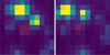 |
Fig. 1 CCD post-stamp images from TESS TPF data, shown for TIC 33770579. The images are from two observing runs: sector 28 (left) and sector 29 (right). Red-hatched squares indicate the TESS pipeline aperture used for extracting the light curve. |
2 Time-series data
The TESS data used in this study were retrieved from the Barbara A. Mikulski Archive for Space Telescopes (MAST)1. We primarily used the Pre-search Data Conditioning flux light curves (PDC-SAP; PDCSAP_FLUX in the FITS files), prepared by the TESS pipeline using optimised apertures (i.e. masks). While the majority of the time-series data we used were collected in the short cadence (SC; 2-minute) mode, we also employed 20 second ultra-short cadence (USC) data, when available, to detect higher frequency signals. For downloading the data, calculating Lomb-Scargle periodograms (VanderPlas 2018), and phase-folding of the light curves, we used the Lightkurve 2.4.2 package (VanderPlas 2018). Since Lightkurve periodograms yielded spurious signals in one instance (see Appendix B), we also used the fnpeaks2 software to calculate the Fourier transform (FT) of the light curves and cross-check the results.
Most light curves required further analysis to determine whether the target star was the source of the observed frequencies. This was necessary because TESS data are obtained using cameras with large 21′′ × 21′′ pixels, which often results in contamination of the target star’s light curve by background stars. The degree of contamination is estimated by the CROWDSAP parameter, which is defined as the fraction of the target star’s flux within the photometric aperture. CROWDSAP values range from 0 to 1 and are provided with the TESS light curves. However, even stars with CROWDSAP values approaching 1 may not be the true origin of the variability. Taking this into account, we utilised target pixel files (TPFs), which encompass the original CCD time-series data for each TESS object, presented in the form of ‘post-stamp’ image cutouts around the objects (Fig. 1). To determine the location of signals (if present in TESS light curves) within the TESS aperture, we used the TESS-Localize software (Higgins & Bell 2023) on TPF data. This software takes the observed frequencies as input parameters and calculates the best-fit locations for the signal sources within the provided TPF. The results are presented as heat maps of the amplitude fits (for the frequency source with the highest signal-to-noise ratio), with the location of the frequency source marked by a black cross (Fig. 2). To estimate the fit quality, the software also provides two main metrics: the relative-likelihood (expressed as a percentage), which estimates the relative probabilities of each star’s location corresponding to the fit location; and the p-values, which assess the hypothesis that the position of each star is consistent with the fit location. Users can also utilise other parameters to evaluate the fit properties in problematic situations (see Pedersen & Bell 2023).
In this work, we considered positive detections to occur when the relative-likelihood was above 60%. Additionally, warnings were raised when the p-values were below 0.1, prompting further checks. These checks typically involved running TESS-Localize on other available seasons, or verifying against other signals found in periodograms. In some cases, to support the TESSLocalize results, we also used TPFs to perform custom aperture photometry on both raw and simple aperture photometry (SAP) fluxes (i.e. fluxes after background removal) using masks different from those used by TESS. This approach can produce improved light curves in conditions such as crowded fields or CCD images affected by light contamination. When a contaminating star was identified, we calculated periodograms for light curves extracted from individual pixels of the TPF frames and compared them with those of the target star to further validate the origin of the detected signal. However, we found that TESS-Localize generally provided more reliable results than our custom TPF light curve analysis. Nevertheless, it is important to note, as highlighted by Pedersen & Bell (2023), that TESSLocalize can sometimes provide inconclusive or inconsistent results across different runs, and therefore cannot be entirely trusted.
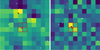 |
Fig. 2 Example heat maps for TIC 33770579 created using TESS-Localize for low-frequency signals (left) and high-frequency signals (right). The target is marked with a red star, and the signal source is indicated with a black cross. The TESS aperture is outlined with red borders around the pixels. The positions of other stars within the frames are marked with white circles. |
3 Light curve analysis and results
Periodograms were computed for both SC and USC data. To identify signals in the amplitude spectra, a detection threshold was applied, defined as five times the signal-to-noise ratio (S / N; see also Baran & Koen 2021, for a discussion on the detection threshold for TESS data). This detection threshold was calculated separately in two frequency regions: a low-frequency range from 0 to 5 d−1, a high-frequency range from 5 to 360 d−1 for SC data and 5–1000 d−1 for USC data. The boundary frequency at 5 d−1 was chosen because sdBV pulsations are not expected below frequencies of approximately 4−5 d−1. It should be noted that USC data typically exhibit lower detection thresholds than SC data when their observational durations are comparable (Huber et al. 2022). However, SC datasets usually contain more observing runs, which improves frequency resolution and typically results in lower overall detection thresholds. Additionally, in the low-frequency range, SC data commonly yield lower periodogram detection thresholds compared to USC data of similar lengths. Thus, SC data were primarily utilised for detecting variability in the 0−360 d−1 frequency range, while USC data were employed to search for signals above ∼ 360 d−1, corresponding to the Nyquist frequency of SC data.
Approximately half of the light curves from the initial sample of 3310 objects exhibited periodogram signals exceeding the assumed detection threshold, in the low and/or high-frequency regions. These were divided into two categories: a group of ‘binary candidates’ that exhibit only low-frequency signals, and a group of ‘pulsating candidates’ that display signals in the high-frequency region or in both the low- and high-frequency regions. Both the light curves and corresponding periodograms were visually inspected to assess photometric variability. Over 300 stars classified as cataclysmic variables in the literature were excluded from the sample, along with the known variable hot subdwarfs identified to date. This refinement reduced the final set of variable hot subdwarfs to 66 objects. Most of these 66 objects fell within the previously defined CMD region (2.26 ≤ MG ≤ 6.11 and GBP−GRP ≤ 0.1), where the majority of known sdBVs are located (Fig. 1 in Uzundag et al. 2024). During the preparation of Paper I, these candidates were either categorised as binaries hosting pulsating hot subdwarfs (reserved for future analysis) or had signals below the detection threshold. A few were inadvertently missed due to human error. However, by using TESS-Localize on TPF data, we were able to attribute variability to only 42 of the 66 analysed objects (Table A.1). The remaining objects appeared to either be non-variable or to be other types of contaminants within our sample of variable objects (see Appendix B).
Among the variable objects, 22 were identified as pulsating sdBs (‘22 pulsating sdBs’ in Table A.1), most of which exhibited multiple signals in the high-frequency region (Fig. A.1). However, three stars – TIC 178626010, TIC 194807290, and TIC 258021652 – were classified as pulsating sdBVs despite their periodograms having only a single frequency whose amplitude exceeded the assumed detection threshold. This classification was based on the absence of subharmonics or harmonics accompanying these signals, along with the presence of additional peaks in the periodograms with signal-to-noise S/N ratios between 4 and 5. For these stars, future TESS observations may help determine whether they exhibit pulsations or are instead members of binary systems. In Table A.1, these stars are marked with the ‘4 S/N’ label in the ‘Signal found’ column.
Pulsating modes of sdBV stars are classified the same way as in Paper I. Therefore, in Table A.1 g-mode pulsators are labelled ‘G’ in the ‘Type’ column when their observed frequencies fall between 5 and 55 d−1 (1571 and 17280 s), p-mode pulsators ‘P’ if the periodogram frequency is above 340 d−1(254 s), and intermediate mode pulsators ‘I’ if their observed frequencies ranged between 55 and 340 d−1 (254 and 1571 s). Binary stars are labelled ‘B’. A hybrid-mode pulsator (‘H’) would need to meet both the G and P classification criteria; however, none were found. Periodograms of pulsating sdB stars are presented in Fig. A.1. For most stars, the frequency range shown spans 0−50 d−1. Three stars exhibiting signals at higher frequencies have their periodograms centred around the visible pulsation modes.
It should be noted that nearly all of the initial ‘pulsating candidates’ exhibited signals in the low-frequency region, indicating that they could be candidates for binaries hosting pulsating hot subdwarf stars. However, low-frequency variability visible in TESS data may be caused by signals associated with the reaction wheel momentum dumps of the TESS telescope. These signals typically occur near 0.3 d−1 and/or at their sub-harmonics and can mimic genuine light curve variations. In fact, in most cases, the low-frequency signals were attributed to background variations (likely caused by reaction wheel momentum dumps), while others were linked to neighbouring stars within the CCD frame. Consequently, the final set of pulsating stars in binary systems has been reduced to only three candidates (one sdOV and two sdBVs). They are listed in Table A.1 as ‘1 pulsating sdO in a binary candidate’ and ‘2 binary + pulsating sdB candidates’. Periodograms for these stars are shown in Fig. A.2, while their phase-folded light curves are presented in Fig. A.6. Pulsation mode frequencies were pre-whitened from the light curves prior to phase-folding.
Table A.1 also lists 13 objects exhibiting single frequencies in the high-frequency region of their periodograms (Fig. A.3). Since sdBVs are typically multi-mode pulsators, we classified these stars as ‘binary candidates’. Of these, two stars show sub-harmonics or harmonic frequencies associated with the highest-amplitude signals. The phase-folded light curves of all 13 objects are shown in Fig. A.6. As shown in this figure, the light curves of five stars (TIC 5816844, TIC 433351247, TIC 466750264, TIC 1228441515, and TIC 239930769) likely exhibit reflection or ellipsoidal light variation, while the variability type of the remaining objects remains uncertain due to noise in the light curves and/or low-amplitude variations. The variability periods corresponding to the observed frequency peaks in the periodograms of the binary candidates are listed in the ‘P[d]’ column of Table A.1.
At the end of Table A.1, we list four objects that may be pulsating hot subdwarfs and/or binaries, referred to in the table as ‘4 low relative-likelihood pulsators/binary candidates’. Given that their TESS-Localize relative-likelihood is below the assumed 60% threshold and their p-values are below 0.1, the classification of these objects should be treated with caution.
Figure 3 illustrates the positions of newly discovered variable hot subdwarfs in the Gaia CMD, shown relative to known pulsating sdBVs from Uzundag et al. (2024) and Baran et al. (2024). The hotter portion of the region below GBP−GRP = 0.1, and between 2.26 ≤ MG ≤ 6.11, defines the adopted search area for pulsating sdBVs, as described in Uzundag et al. (2024).
As shown in the figure, most of the new sdBVs are located within this search region. These objects were excluded from the search in Paper I, mainly due to binary signatures identified in their periodograms. In the current analysis, however, the sources of the low-frequency signals were attributed to variable backgrounds in the CCD data or to background stars. As a result, these stars were reclassified as pulsators. Three sdBVs TIC 178626010, TIC 270712778, and TIC 402894814 are located outside the search region, and may indicate the presence of potential companions.
The position of the binary candidate with a pulsating sdO (TIC 5816844) in the CMD suggests the presence of a cooler companion, as sdOs are expected to be hotter than sdBs and should therefore appear on the hotter side of the sdBV search region. Also, one of the stars (TIC 170888817) from the ‘binary + pulsating sdB candidates’ group lies on the cooler side of the vertical line, where binary companions to sdB stars are often expected.
About half of the stars classified as binary candidates are located within the pulsating sdBV region. All four stars from the ‘low-likelihood pulsator/binary candidates’ group also fall within this region, underscoring the need for further investigation into their true nature.
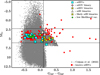 |
Fig. 3 Newly discovered sdB variables in the Gaia CMD. Hot subdwarf candidates from Culpan et al. (2022) are shown as grey dots, and known pulsating sdBVs as red dots. The adopted search region for pulsating hot subdwarfs lies on the hotter side of the vertical line and between the two horizontal lines. |
4 Spectroscopic observations
In addition to the light curve analysis, follow-up spectroscopic observations were conducted for nine stars from the ‘pulsating sdBs’ group, one star from the ‘binary+pulsating sdB’ group and one from the ‘low relative-likelihood pulsator/binary candidates’ group (marked with asterisks in Table A.1) to determine their atmospheric parameters. The observations were carried out using three different instruments, with details provided in Table 1.
TIC 28522887, TIC 326559609, and TIC 207111243 were observed with the European Southern Observatory (ESO) Faint Object Spectrograph and Camera v.2 (EFOSC2; Buzzoni et al. 1984) mounted at the Nasmyth B focus of the New Technology Telescope (NTT) at La Silla Observatory. The data from the EFOSC2 spectrograph were processed and analysed using standard PyRAF procedures. Bias and flat-field corrections were applied initially. Then, pixel-to-pixel sensitivity variations were eliminated by dividing each pixel by the response function. Subsequently, wavelength calibrations were applied using spectra from the internal He-Ar lamp. Finally, flux calibration was carried out using standard stars. The S/N of the final spectra ranged between 40 and 80.
TIC 27782233 was observed with the Isaac Newton Telescope (INT), a 2.54 m (100 in) optical telescope operated by the Isaac Newton Group of Telescopes at the Roque de los Muchachos Observatory on La Palma, 14 September 2022, with each observation having an exposure time of 1800 seconds. We utilised the Intermediate Dispersion Spectrograph (IDS) longslit spectrograph with the R 400 V grating (R = 1452) and a 1.5 arcsecond slit. This configuration provides a resolution of about 3.5 Å. Bias and flat field corrections were applied to the data, and wavelength calibration was performed using Cu-Ar+ Cu-Ne calibration lamp spectra. The S/N of the final spectra is approximately 100.
We later obtained data for TIC 154432267, TIC 258021652, TIC 348825375, TIC 310930161, TIC 387884969, TIC 48085434, and TIC 341157482 with the INT on 15 and 16 June 2024 with the R1200B grating and a 1.04 arcsecond slit, providing a resolution of 0.96 Å. Arc calibration exposures were obtained during the target observations, with S/N values of approximately 30 in the continuum of each spectrum. Bias and flat fields were taken before the night and the spectra were flux calibrated with spectrophotometric flux standards. The data were reduced with the MOLLY package (Marsh 2019) and spectra were extracted using the method outlined in Marsh (1989).
To derive atmospheric parameters from spectra, we employed the data-driven steepest-descent fitting procedure implemented in XTGRID (Németh et al. 2012), specifically designed to automate the spectral analysis of early-type stars using TLUSTY and SYNSPEC (Hubeny & Lanz 2017) non-local thermodynamic equilibrium stellar atmosphere models. The method employs an iterative chi-square minimisation approach to fit the observed data. Starting from an initial model, the algorithm converges on the best-fit solution through successive approximations along the chi-square gradient. To reduce systematic effects resulting from imperfect blaze function correction, spectrograph flexure or flux inconsistencies due to vignetting or slit loss, the models were compared with observations using a piecewise normalisation. Accurate parameter determination for hot stars depends critically on both the completeness of included opacity sources and on the treatment of non-local thermodynamic equilibrium effects. We found that TLUSTY models, characterised by H and He composition, yield reliable results within the constraints of spectral resolution, coverage, and signal-tonoise ratio of the survey data. XTGRID dynamically computes the required TLUSTY atmosphere models and synthetic spectra, incorporating a recovery mechanism to tolerate convergence failures and accelerate convergence convergence on a solution whit a minimal number of model evaluations. Figure 4 shows the best fits for the spectra of the 11 newly discovered variable sdB stars. Only the blue portion of the spectra is shown for the EFOSC2 and low-resolution IDS data. The surface parameters are listed at the top of Table 2. Parameter uncertainties were evaluated by mapping the chi-square statistics around the solution. Each parameter was varied independently until the 60% confidence limit was reached. Correlations near the best-fit values were incorporated into the final results for the surface temperature and gravity. Geometric distances and their uncertainties, listed in Table 2 were collected from Bailer-Jones et al. (2021) catalogue.
XTGRID also collects photometric measurements from the VizieR Photometry Viewer Tool3 to sample the spectral energy distribution (SED) of the target and compare it with its spectral model. Since the SED is sensitive to the infrared excess caused by FGK-type companions, it was used to assess the binarity of the 11 spectroscopically observed objects. However, for compact or low-mass companions on wide orbits, the flux contribution is too low to reliably assess binarity from the SED alone, making radial velocity measurements essential. Figure 5 shows SEDs for the 11 objects analysed in this study. The negligible infrared excess observed rules out the presence of F-, G-, or K-type companions for all these stars. With a proper absolute calibration of the surface parameters, interstellar extinction, and distances, the SEDs can be used to determine the mass, radius, and luminosity of stars. In our case, the low spectral resolution, limited coverage, and relatively low S/N of the spectra introduce significant systematic uncertainties in the surface gravity; therefore, we report only the mean mass of the 11 stars, 〈M〉=0.39 ± 0.15 M☉.
Atmospheric parameters, both determined in this work and those collected from SIMBAD, were used to verify the pulsational variability of the stars. To achieve this, we plotted the stars listed in Table 2 on a log g versus Teff diagram (Fig. 6) and compared their positions with those of known pulsating sdBVs.
Interestingly, the figure reveals two stars (TIC 77477081 and TIC 161358962) located in the region where p-mode pulsators are typically found (Teff>∼ 35 000 K). Of these, only TIC 77477081 exhibits an intermediate pulsating mode, while TIC 161358962 displays a single g-mode in its periodogram (see Appendix A for additional comments on this star). The remaining pulsating and other variable sdBs have effective temperatures below 30 000 K, covering the region where most g-mode pulsators are found. In this context, stars identified as ‘binary candidates’ and ‘low relative-likelihood pulsator/binary candidates’ might actually be pulsators and require further observations to confirm the nature of their variability. Four stars with the lowest Teff (TIC 27782233, TIC 28522887, TIC 154432267, and TIC 341157482) appear to better define the observed pulsational instability region for sdBV stars at lower temperatures (solid red squares on the right side of Fig. 6).
Using the Teff values determined from both the literature and our own observations, we created Fig.7, which shows the dependence of pulsation frequency on temperature for 16 sdBVs listed in Table 2. As the pulsational frequency, we used the frequency representing the weighted mean of the frequencies detected in the periodograms of the stars, with the amplitudes serving as weights. The frequency uncertainties are defined as half the range between the lowest and highest frequencies detected. For three stars (TIC 258021652, TIC 194807290, and TIC 184607974), the frequency range was determined based on the lowest and highest frequencies detected above the 4 S/N detection threshold (otherwise only single frequencies would have been detected; see Table A.1). The point in the top right corner of the Fig. 7 corresponds to TIC 161358962, which exhibits a single frequency at 38.3439 d−1. This star was classified as a g-mode pulsator based on the assumption that the observed frequency is too high to be associated with an orbital frequency (see Appendix A).
As shown in Fig.7, most points follow a well-known trend in which pulsation frequencies increase with higher temperatures (see also Uzundag et al. 2021, Fig. 1). The only exceptions are the points marked with circular symbols, corresponding to TIC 326559609 and TIC 258021652. These two stars deviate from the fit line by more than three times their frequency errors (see also notes on these cases in Appendix A). In summary, the newly identified pulsating sdBs appear to be correctly classified based on their spectral parameters, the analysis and the plots presented.
Spectroscopic data obtained for the 11 variable sdBs studied in this work.
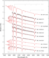 |
Fig. 4 Best-fit TLUSTY models (red) for the collection of observed spectra (grey) of the newly discovered variable sdB stars, arranged by increasing Teff from the bottom. The observed fluxes were scaled to match the final models. Surface parameters were determined from our spectroscopic observations (Table 2). |
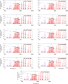 |
Fig. 5 SED plots for 11 stars (Tables 1 and 2) whose spectral data were collected in this work. The blue curves represent the model fits to the spectra, while the SED points are marked with black circles. The filter transmissions of the photometric systems are shown as pink to reddish shaded regions in the background. The photometric system bands are labelled (from left to right in each SED plot) as FUV and NUV for GALEX; u, g, r, i, and z for SDSS; BP and RP for Gaia; J, H, and Ks for 2MASS; and W1 and W2 for WISE. The vertical grey lines mark the wavelengths where the model was normalised to the photometric measurements. |
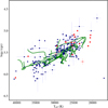 |
Fig. 6 Location of the spectroscopically identified pulsating sdB stars in the Teff−log g plane. Known pulsating sdBs, collected from Uzundag et al. (2024) and Baran et al. (2024), are shown as blue dots. Newly discovered pulsating sdBs, for which atmospheric parameters are known (Table 2), are represented by solid red squares. Open symbols indicate variables from the ‘binary candidates’ and ‘low relativelikelihood pulsators/binary candidates’ groups. Evolutionary models from Uzundag et al. (2021) for MZAHB = 0.467, 0.4675, 0.468, 0.4685, and 0.47 M☉ are shown in green. |
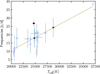 |
Fig. 7 Frequency vs Teff for the 16 sdBV identified as g-mode pulsators in this study for which Teff is known. Pulsating sdBs identified based on frequency peaks exceeding the 4 S/N detection threshold are shown as solid symbols. The circles represent two outliers, and the line is the least-squares fit to all points. |
5 Conclusions
Paper I (Uzundag et al. 2024) focused on the search for pulsating sdBVs within the region defined by the distribution of 256 known pulsating sdBVs in the Gaia CMD. At that time, pulsating hot subdwarfs in binary systems and those outside the search region were excluded and left for future investigation. Here, in Paper II, we present the results of our search for the remaining pulsating hot subdwarfs, regardless of their location in the CMD or binarity. To achieve this, we prepared a sample of approximately 3300 TESS PDC-SAP light curves of hot sub-luminous stars. These were selected from the TESS Input Catalog (Stassun et al. 2019) and cross-matched with the Culpan et al. (2022) catalogue, which is based on Gaia EDR3 (Gaia Collaboration 2021).
After analysing the light curves and periodograms, and reviewing the literature, we narrowed the sample to 66 new variable candidates that exhibit high-frequency signals or signals in both the low- and high-frequency regions of their periodograms. Despite our initial expectation of finding new pulsating hot subdwarf candidates in binary systems, further analysis of the TPF light curves (using TESS-Localize software) showed this was not the case. We determined that variability can be attributed to the target stars in 42 cases. Of these, 22 appear to be pulsating sdBs and 3 are candidates for binaries containing a pulsating hot subdwarf component. Four hot subdwarfs have low relative-likelihood values (below 60%) for the fit of the signal source location (see the TESS-Localize parameters description in Sect. 2). All but three of the newly found sdBVs fall within the Gaia CMD region for pulsating sdBVs (Fig. 3), as defined in Paper I (Uzundag et al. 2024). This supports the validity of the Uzundag et al. (2024) selection method in future searches for pulsating sdBVs.
For 11 objects from Table A.1 (10 sdBVs and 1 low-likelihood pulsator/binary candidate, marked with asterisks in the table) we obtained spectral observations (Table 1) and determined their log g, Teff, and log (nHe/nH). Additionally, we collected log g and Teff values from the literature for 10 stars (Table 2). Collectively, these 21 objects lie within or near the Teff versus log g region occupied by known pulsating sdBs, as illustrated in Fig. 6.
Stars worth mentioning in addition include a candidate for a pulsating sdO star in a binary system (TIC 5816844) and four sdBVs (TIC 27782233, TIC 310930161, TIC 341157482, and TIC 387884969). These four sdBVs exhibit a richer pulsation spectrum than the other sdBVs listed in Table A.1, making them potentially important objects for asteroseismic analysis. The spectra of all objects for which we determined surface parameters (Table 2) do not show any infrared excess. This may be due to the wavelength range covered with spectrographic observations. Notably, the spectra obtained in this work do not cover wavelengths beyond 5400 Å (Fig. 4).
Additionally, we collected SEDs from SIMBAD VizieR (Wenger et al. 2000) and compared them with our spectral models; they show no significant infrared excess (Fig. 5). In fact, the SEDs for all 11 stars observed in this work are consistent with single stars, although this does not rule out binaries with compact, late-type (M), or substellar companions. Since no significant flux contribution from a companion is observed, FGK-type companions can be excluded, as they would be evident in the spectrum. The small discrepancies in the SEDs for TIC 207111243, TIC 258021652, and TIC 387884969 may be due to interstellar reddening. All stars listed in Table A.1 were also cross-matched with the Gaia Collaboration (2023) non-single star catalogue to identify binaries. However, none were found.
Finally, it is worth noting that over the years of TESS operations, the discovery rate of pulsating hot subdwarfs identified using TESS photometric data has decreased. This study, for example, identified only 22 pulsating sdBVs, compared to the 61 reported in Paper I. Many of the past discoveries still require confirmation of their variability due to the large pixel size of the TESS CCD cameras, necessitating verification of the signal source (for example, see the notes on TIC 210196125 in Appendix B). Previously, this was accomplished using TESS TPF data and pixel-by-pixel light curve analysis. Currently, TESS-Localize is considered the most reliable software for assessing target variability within TESS apertures. While TESS-Localize can produce inconsistent outcomes for the same object across different runs, it remains an improvement over earlier methods. In cases where variability is uncertain, additional photometric data from higher-resolution CCD cameras are required for confirmation. Furthermore, many of the variables identified in this and previous studies still require spectroscopic confirmation, as this remains the only definitive method for verifying both the spectral type and variability of the objects. Future follow-up observations should prioritise these efforts.
In summary, our results significantly expand the sample of known pulsating hot subdwarfs and binary candidates, underscoring the crucial role of combining space-based photometry with ground-based follow-up observations to deepen our understanding of the formation and evolution of these compact stars.
Acknowledgements
M.U. gratefully acknowledges funding from the Research Foundation Flanders (FWO) by means of a junior postdoctoral fellowship (grant agreement No. 1247624N). P.N. acknowledges support from the Grant Agency of the Czech Republic (GAČR 22-34467S). H.D. is supported by the Deutsche Forschungsgemeinschaft (DFG) through grant GE2506/17-1. I.P. acknowledges support from a Royal Society University Research Fellowship (URF\R1\231496). This research has used the services of www.Astroserver.org under reference M323OZ. Software used: Astropy (Astropy Collaboration 2013, 2018), Astroquery (Ginsburg et al. 2019), lightkurve (Lightkurve Collaboration 2018), Matplotlib (Hunter 2007), NumPy (Harris et al. 2020), and SciPy (Virtanen et al. 2020), TLUSTY and SYNSPEC (Hubeny & Lanz 2017), XTGRID (Németh et al. 2012), TESS-LOCALIZE (Higgins & Bell 2023).
Appendix A Notes, tables, periodograms, and phase-folded light curves
This appendix includes remarks on the new variable hot subdwarfs (marked with the letter A in the notes column of Table A.1), along with periodograms for all stars listed in that table (Figs. A.1, A.2, A.3, and A.4), and phase-folded diagrams for binary candidates (Fig. A.6). A supplementary table (Table A.2) provides the sectors and number of runs used for the light curve analysis of the stars from Table A.1.
Notes to Table A.1
TIC 5816844: The sdO type of the star was determined by Kilkenny et al. (1977). Its periodogram (Fig. A.2) calculated from USC data reveals a doublet of frequencies at 623.336323 d−1 and 623.424059 d−1, along with a strong signal near 0.362743 d−1, which is close to the frequency of TESS reaction wheel momentum dumps. The low-frequency range signal exhibits variable amplitude; in the SC data from sector 37 (observed in 2021), the amplitude is twice as high as in sector 63 (observed in 2023). The peak remains above the adopted detection threshold after detrending the light curve with a 3-day period. Since detrending did not eliminate the signal, we associate the 0.362743 d−1 frequency with the target flux. The relative-likelihood and p-value are close to 100% and ∼ 0.5, respectively, when TESS-Localize is run using the low-frequency signal and sector 37 SC data. This could confirm that the source of the low frequency variation is located in the target star; however, TESS-Localize fails to run on the sector 63 data. The star’s phase-folded light curve (Fig. A.6) suggests the presence of a reflection effect or ellipsoidal variation. We also verified that in the Gaia CMD, the star lies below the MS, and the observed period cannot be associated with any MS pulsators such as Slowly Pulsating B-type or Beta Cephei stars.
TIC 27782233: The star is a confirmed sdB with LAMOST spectra and an estimated Teff of 21 420 K Luo et al. (2021). From our own spectral observations (Table 2) the Teff is slightly lower (20670 K), while log g value (5.26) agrees with the LAMOST analysis. A low-frequency signal at 1.19808 d−1 in the light curve periodogram was attributed to a neighbouring star (Gaia DR3 1879544866315726336, relative-likelihood 100%). High-frequency signals (11.364310, 11.676852, 12.025258, 12.788679 d−1) are associated with the target star’s pulsations and likely form a g-mode quintuplet with one missing component (m = +1). If this interpretation is correct, the frequency spacing within the quintuplet suggests a rotational period of approximately 2.4 d. Additionally, the highest amplitude frequency at 12.025258 d−1 has a sub-harmonic, indicating a possible binary nature of the target star.
TIC 161358962: The source of a single frequency at 38.3439 d−1 (Fig. A.1) was attributed to the star by TESS-Localize. If this frequency is interpreted as the orbital frequency, the star would belong to the class of shortest-period binaries, with a period of 0.0261 d (the current record holder is ZTF J213056.71+442046.5 or TIC 240326669 (Kupfer et al. 2020), with an orbital frequency of approximately 37 d−1). In the case that the observed frequency is due to ellipsoidal light variation, the orbital frequency would be half of the observed value. However, we do not observe any sub-harmonics or harmonics of the 38.3439 d−1 frequency. The phase-folded light curve at the period corresponding to the sub-harmonic (0.052159 d ; Fig. A.5) shows low-amplitude variations, providing no clear evidence for ellipsoidal modulation. Therefore, we classified the star as pulsating, although this classification should be treated with caution.
TIC 192733455: The periodogram of the star’s light curve reveals a single frequency at 7.3655 d−1. No sub- or harmonics are detected. While the phase-folded light curve appears noisy, its binned profile reveals no reflection or ellipsoidal-like profile. This suggests variability potentially caused by g-mode pulsations or the rotation of a secondary component. On the other hand, the location of the star outside the CMD region associated with pulsating sdBVs (Fig. 3, yellow cross at ∼ 0.4) supports a binary nature of the star.
TIC 258021652: The position of this object in Fig. 7 (represented by a solid circle) shows that its detected frequency is consistent with that of higher-temperature sdBVs (near 30 000 K), while Teff derived from our observations (Table 2) is 25 370 K. However, as the trend in Fig. 7 cannot be reliably used to estimate Teff, the observed departure of the star’s parameters from the trend should be addressed in future studies.
TIC 310930161: The star shows a low-frequency signal at 2.6851 d−1. For this signal, TESS-Localize provides inconsistent results. The relative likelihood is only 6.3% and the p-value is 0.5, observed in just one of four seasons. In the remaining seasons, the source of the variation is not localised within the star’s aperture.
TIC 326559609: Based on the position of the star in Fig. 7 (represented by an open circle), its pulsation frequency fits better with low-temperature sdBVs (around 20000 K). The star’s periodogram (Fig. A.4) reveals a weak frequency signal near 5 d−1 and a stronger signal near 10 d−1. The low-amplitude signal cannot be analysed using TESS-Localize due to its faintness. TESS-Localize reports a relative-likelihood of approximately 54% for the strong signal in the first TESS run for the star, but 0% in the second, leaving the signal’s source undetermined. Consequently, we classified this star as a ‘low relative-likelihood pulsator/binary candidate’ (Table A.1). However, if the star is indeed the source of the strong signal, its deviation from the general frequency trend in Fig. 7 may instead suggest it is a binary system.
TIC 433351247: SIMBAD classifies this star as a δ Sct. However, the star is located away from the MS in the CMD, and the light curve periodogram shows a single frequency at 19.1652 d−1 along with its harmonic (Fig. A.3). The phase-folded light curve of the star exhibits a reflection effect. Additionally, the relative-likelihood for this star is 77% (p-value is 0.16), which is the lowest among all the relative-likelihoods calculated for the stars listed in Table A.1 (excluding the ‘low relative-likelihood pulsator/binary candidates’). Therefore, one cannot exclude the possibility that the actual variable is the neighbouring star Gaia DR3 141419258581441536.
TIC 456643055: The source of the highest peak in the periodogram, located at 6.6449 d−1 (Fig. A.1), lies outside the star’s aperture. The remaining frequencies between 12−16 d−1 are attributed to the pulsations originating from the target.
Newly discovered variable hot subdwarfs.
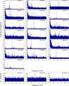 |
Fig. A.1 Normalised Lomb-Scargle periodograms for the 22 newly discovered pulsating sdBVs listed in Table A.1. The normalisation is based on the highest peak in the high-frequency range. Horizontal red and orange lines indicate the assumed detection thresholds for the low- and high-frequency ranges, respectively. Note that the three periodograms at the bottom are shown in different frequency ranges. None of the low-frequency range signals are attributed to the presented objects; these signals are caused by background stars or background variations. |
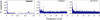 |
Fig. A.2 Normalised Lomb-Scargle periodograms for one pulsating sdO star candidate and two sdBV candidates in binary systems. Horizontal red and orange lines indicate the detection thresholds for the low- and high-frequency ranges, respectively. Periodogram normalisation is based on the highest peak. Note the sdO star’s periodogram division into two frequency ranges: 0−10 d−1 and 622−624 d−1. |
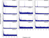 |
Fig. A.3 Normalised Lomb-Scargle periodograms for 13 ‘binary candidates’. Horizontal red and orange lines indicate the assumed detection thresholds for the low- and high-frequency ranges, respectively. The normalisation of the periodograms is based on the highest peak in the high-frequency range. |
Appendix B False positives, contaminants, and notable cases
In Table B.1 we list 21 variable hot subdwarf candidates for which variability was attributed to background stars or background variations (false-positive detections). In addition, we include below remarks on three other hot subdwarf candidates: TIC 280678642, TIC 210196125, and TIC 131040362.
A periodogram of TIC 280678642 reveals a broad excess of power and several frequency peaks between 50−100 d−1 that are above the detection threshold in one season. This applies when the threshold is calculated over the full 5−360 d−1 range. However, when the detection threshold is recalculated specifically for the 50−100 d−1 range, no significant signals are detected. In the second of the two available seasons, neither a power excess nor any peaks above the detection threshold are present. In the periodogram calculated from the combined two-season data, a narrow power excess is visible but remains well below the detection threshold. Therefore, the star was not classified as a variable until additional data confirm otherwise.
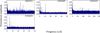 |
Fig. A.4 Normalised Lomb-Scargle periodograms for ‘low relative-likelihood pulsator/binary candidates’. Note that for TIC 35500220 the frequency range is 0−250 d−1. Horizontal red and orange lines indicate the assumed detection thresholds for the low- and high-frequency ranges, respectively. Periodogram normalisation is based on the highest-amplitude frequency peaks. |
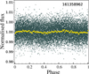 |
Fig. A.5 Phase-folded light curve on a 0.052159 d period for TIC 161358962. Phase zero is arbitrarily set to the first data point. The yellow curve represents the binned phase-folded light curve. |
The variability of TIC 210196125 (classified as sdO by Downes 1986) was traced to a ∼ 12.4 magnitude neighbouring star (TIC 210196124) that, according to SIMBAD, is a binary or multiple system. However, the low-frequency signal at 1.257 d−1 (0.7953 d) observed in PDC-SAP flux is not detected in any season when periodograms are calculated from the light curve extracted directly from TPFs. Therefore, the star binarity remains to be verified. Also, using the light curve extracted from the aperture around the neighbouring star and its colour from SIMBAD (B−V=0.35 mag), we conclude that high-frequency peaks between 25 and 50 d−1 (Fig. B.1) are consistent with the δ Scuti star pulsation pattern, which can mimic g-mode pulsations in sdBV stars.
We also identified a contaminant object TIC 131040362 listed in the Culpan et al. (2022) catalogue of hot subdwarf candidates. This isolated star exhibits two frequencies at 0.82 and 5.8749 d−1 in its light curve periodogram. Both frequencies were attributed to the target with a relative-likelihood of approximately 100% and a p-value greater than 0.1. While SIMBAD classifies the star as a B2III type, its position in the Gaia CMD places it above and to the left of the tip of the MS (Fig. B.2). Considering its spectral type, location relative to other B-type stars in the CMD, and its variability, the target is most likely a B-type variable (Pedersen et al. 2019; Burssens et al. 2020).
In one instance, we encountered an issue with the spectral type classification of the star TIC 207085743 and the Lightkurve software. Although the star is classified as a variable RR Lyrae type in SIMBAD, Van Grootel et al. (2021) identified it as an sdO star. This classification was later confirmed (or reiterated) by Schaffenroth et al. (2022) in their Table 4 (‘All confirmed systems with light variations’). The periodogram of TIC 207085743 (calculated using the 120-second integration time data from sectors 03, 02, 29, and 69), shows a strong signal at 2.359 d−1 (with an amplitude of 150.8082 ppt compared to the detection threshold near 15 ppt). This appears to confirm the RR Lyrae-type variability noted in earlier studies.
In addition to the signal at 2.359 d−1, the light curve periodogram shows two peaks in the high-frequency range at 345.687776 and 350.405975 d−1. Further investigation revealed that these high-frequency signals were false and were introduced by the Lightkurve package used to calculate Lomb-Scargle periodograms, likely due to the astropy package on which Lightkurve relies. This discovery was made accidentally when we calculated a FT for this star using different software (fnpeaks; see Sect. 2) and the same data (i.e. BJD[d], Flux[ppt]). The fnpeaks FT does not show any peaks in the high-frequency region. Therefore, the object is not a pulsating sdO star, and we can only confirm the previously observed variability associated with the star. A similar analysis was performed for all other stars in our hot subdwarf sample to verify the results obtained with the lightkurve software. No issues were identified in the data for the other objects.
The false signals in periodograms can occur when the oversample_factor parameter is set to 10 or 20 in the lightkurve.to_periodogram function call. Since the Lightkurve package utilises astropy for Lomb-Scargle periodogram calculations, the issue may lie within astropy rather than Lightkurve itself. It seems that the false signals do not manifest when the oversample_factor is set to values other than 10 or 20. However, our periodogram calculations were checked only for oversample_factor values ranging from 5 to 30. Whether the issue arises for other oversample_factor values has not been verified. While false signals were not detected in periodograms generated with other than 10 or 20 oversample_factor values, we are presenting this problem to alert users.
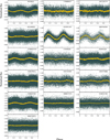 |
Fig. A.6 Phase-folded light curves of binary candidates. Top row (three panels): Pulsating hot subdwarfs in binary systems. Remaining panels: Other binary candidates. The light curves are phase-folded on twice the period (as listed in the P[d] column of Table A.1). Phase zero is arbitrarily set to the first data point. Yellow curves represent binned phase-folded light curves. |
Available SC and USC observing runs used in this study.
TIC numbers of hot subdwarf candidates with falsepositive detections of variability.
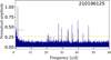 |
Fig. B.1 Normalised periodogram calculated for the sdO star TIC 210196125, displayed over the frequency range 1−60 d−1. Horizontal dashed lines indicate detection thresholds for the low (red) and high (orange) frequency ranges. The pulsation modes visible in the plot originate from a neighbouring δ Scuti star. |
Below is a snippet of our Python code (executed in a Jupyter notebook) used for downloading a light curve and performing periodogram calculations. The code downloads four seasons of SC (120 sec integration time) data for sectors 03 (year 2018), 02 (year 2018), 29 (year 2020), and 69 (year 2023). After stitching the light curves from all seasons and outlier removal, it calculates the periodogram between 0.0001−360 d−1 and plots the results. One should not see any signals above the horizontal dashed line (orange), which is the detection threshold for the periodogram. However, after replacing 7 with 10 (or 20) in the oversample_factor value (see the ‘perg=…’ line in the code), two signals at 345.687776 and 350.405975 d−1 should appear above the ∼ 0.9 ppt detection threshold.
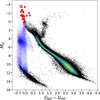 |
Fig. B.2 Position of TIC 131040362 (yellow star) in the CMD. Culpan et al. (2022) catalogue hot subdwarf candidates are marked with blue dots. Red filled circles represent stars of spectral types B1V to B8II, most of which are variable. |
# Python code:
import lightkurve as lk
import matplotlib.pyplot as plt
lk_searchresult=lk.search_lightcurve(“TIC 207085743”, exptime=120)
lk_lc=lk_searchresult.download_all()
print(lk_lc) #prints information on the collected data.
lk_a=(lk_lc[0:len(lk_lc)].stitch(lambda x: x.remove_nans().remove_outliers(sigma=5).normalize())-1.)*1000.
perg = lk_a.to_periodogram(minimum_frequency=0.00001,
maximum_frequency=360, oversample_factor=7)
ax=perg.plot(color=“blue”,linewidth=1,label=tic,ylabel=
“Power”, xlabel=“Frequency [c/d]”)
plt.axhline (y=0.9,linewidth=1,color=“orange”,
linestyle=“dashed”)
ax.set_xlim(150,360)
ax.set_ylim(−0.15,5)
plt.show()
References
- Astropy Collaboration (Robitaille, T. P., et al.,) 2013, A&A, 558, A33 [NASA ADS] [CrossRef] [EDP Sciences] [Google Scholar]
- Astropy Collaboration (Price-Whelan, A. M., et al.,) 2018, AJ, 156, 123 [Google Scholar]
- Bailer-Jones, C. A. L., Rybizki, J., Fouesneau, M., Demleitner, M., & Andrae, R., 2021, AJ, 161, 147 [Google Scholar]
- Baran, A. S., & Koen, C., 2021, Acta Astron., 71, 113 [Google Scholar]
- Baran, A. S., Van Grootel, V., Østensen, R. H., et al. 2023, A&A, 669, A48 [NASA ADS] [CrossRef] [EDP Sciences] [Google Scholar]
- Baran, A. S., Charpinet, S., Østensen, R. H., et al. 2024, A&A, 686, A65 [NASA ADS] [CrossRef] [EDP Sciences] [Google Scholar]
- Burssens, S., Simón-Díaz, S., Bowman, D. M., et al. 2020, A&A, 639, A81 [NASA ADS] [CrossRef] [EDP Sciences] [Google Scholar]
- Buzzoni, B., Delabre, B., Dekker, H., et al. 1984, The Messenger, 38, 9 [NASA ADS] [Google Scholar]
- Charpinet, S., Van Grootel, V., Reese, D., et al. 2008, A&A, 489, 377 [NASA ADS] [CrossRef] [EDP Sciences] [Google Scholar]
- Copperwheat, C. M., Morales-Rueda, L., Marsh, T. R., Maxted, P. F. L., & Heber, U., 2011, MNRAS, 415, 1381 [Google Scholar]
- Culpan, R., Geier, S., Reindl, N., et al. 2022, A&A, 662, A40 [NASA ADS] [CrossRef] [EDP Sciences] [Google Scholar]
- Downes, R. A., 1986, ApJS, 61, 569 [NASA ADS] [CrossRef] [Google Scholar]
- Ekström, S., Georgy, C., Eggenberger, P., et al. 2012, A&A, 537, A146 [Google Scholar]
- Gaia Collaboration (Brown, A. G. A., et al.,) 2021, A&A, 649, A1 [NASA ADS] [CrossRef] [EDP Sciences] [Google Scholar]
- Gaia Collaboration (Vallenari, A., et al.,) 2023, A&A, 674, A1 [NASA ADS] [CrossRef] [EDP Sciences] [Google Scholar]
- Ge, H., Tout, C. A., Chen, X., et al. 2022, ApJ, 933, 137 [NASA ADS] [CrossRef] [Google Scholar]
- Geier, S., Dorsch, M., Pelisoli, I., et al. 2022, A&A, 661, A113 [NASA ADS] [CrossRef] [EDP Sciences] [Google Scholar]
- Ginsburg, A., Sipőcz, B. M., Brasseur, C. E., et al. 2019, AJ, 157, 98 [Google Scholar]
- Green, E. M., Fontaine, G., Hyde, E. A., For, B. Q., & Chayer, P., 2008, in Astronomical Society of the Pacific Conference Series, 392, Hot Subdwarf Stars and Related Objects, eds. U. Heber, C. S. Jeffery, & R. Napiwotzki, 75 [Google Scholar]
- Han, Z., Podsiadlowski, P., Maxted, P. F. L., Marsh, T. R., & Ivanova, N., 2002, MNRAS, 336, 449 [Google Scholar]
- Han, Z., Podsiadlowski, P., Maxted, P. F. L., & Marsh, T. R., 2003, MNRAS, 341, 669 [NASA ADS] [CrossRef] [Google Scholar]
- Harris, C., Millman, K., van der Walt, S., et al. 2020, Nature, 585, 357 [NASA ADS] [CrossRef] [Google Scholar]
- Heber, U., 1986, A&A, 155, 33 [NASA ADS] [Google Scholar]
- Heber, U., 2009, ARA&A, 47, 211 [Google Scholar]
- Heber, U., 2016, PASP, 128, 082001 [Google Scholar]
- Higgins, M. E., & Bell, K. J., 2023, AJ, 165, 141 [NASA ADS] [CrossRef] [Google Scholar]
- Hubeny, I., & Lanz, T., 2017, arXiv e-prints, [arXiv:1706.01859] [Google Scholar]
- Huber, D., White, T. R., Metcalfe, T. S., et al. 2022, AJ, 163, 79 [NASA ADS] [CrossRef] [Google Scholar]
- Hunter, J. D., 2007, Comput. Sci. Eng., 9, 90 [NASA ADS] [CrossRef] [Google Scholar]
- Iben, Icko, J. 1990, ApJ, 353, 215 [NASA ADS] [CrossRef] [Google Scholar]
- Jeffery, C. S., Miszalski, B., & Snowdon, E., 2021, MNRAS, 501, 623 [Google Scholar]
- Kilkenny, D., Hill, P. W., & Brown, A., 1977, MNRAS, 178, 123 [Google Scholar]
- Kilkenny, D., Heber, U., & Drilling, J. S., 1988, South Afr. Astron. Observ. Circ., 12, 1 [Google Scholar]
- Kupfer, T., Bauer, E. B., Marsh, T. R., et al. 2020, ApJ, 891, 45 [Google Scholar]
- Lei, Z., Zhao, J., Németh, P., & Zhao, G., 2019, ApJ, 881, 135 [NASA ADS] [CrossRef] [Google Scholar]
- Lightkurve Collaboration (Cardoso, J. V. d. M., et al.) 2018, Lightkurve: Kepler and TESS time series analysis in Python, Astrophysics Source Code Library [record ascl:1812.013] [Google Scholar]
- Luo, Y., Németh, P., Wang, K., Wang, X., & Han, Z., 2021, ApJS, 256, 28 [NASA ADS] [CrossRef] [Google Scholar]
- Marsh, T. R., 1989, PASP, 101, 1032 [Google Scholar]
- Marsh, T., 2019, molly: 1D astronomical spectra analyzer, Astrophysics Source Code Library [record ascl:1907.012] [Google Scholar]
- Maxted, P. F. L., Heber, U., Marsh, T. R., & North, R. C., 2001, MNRAS, 326, 1391 [CrossRef] [Google Scholar]
- Miller Bertolami, M. M., Althaus, L. G., Unglaub, K., & Weiss, A., 2008, A&A, 491, 253 [NASA ADS] [CrossRef] [EDP Sciences] [Google Scholar]
- Moni Bidin, C., Casetti-Dinescu, D., Girard, T., et al. 2017, MNRAS, 466, 3077 [NASA ADS] [CrossRef] [Google Scholar]
- Napiwotzki, R., Karl, C. A., Lisker, T., et al. 2004, Ap&SS, 291, 321 [NASA ADS] [CrossRef] [Google Scholar]
- Németh, P., Kawka, A., & Vennes, S., 2012, MNRAS, 427, 2180 [Google Scholar]
- Pedersen, M. G., & Bell, K. J., 2023, AJ, 165, 239 [NASA ADS] [CrossRef] [Google Scholar]
- Pedersen, M. G., Chowdhury, S., Johnston, C., et al. 2019, ApJ, 872, L9 [Google Scholar]
- Pelisoli, I., Vos, J., Geier, S., Schaffenroth, V., & Baran, A. S., 2020, A&A, 642, A180 [NASA ADS] [CrossRef] [EDP Sciences] [Google Scholar]
- Ratzloff, J. K., Barlow, B. N., Németh, P., et al. 2020, ApJ, 890, 126 [NASA ADS] [CrossRef] [Google Scholar]
- Ricker, G. R., Winn, J. N., Vanderspek, R., et al. 2015, J. Astron. Telesc. Instrum. Syst., 1, 014003 [Google Scholar]
- Saffer, R. A., Bergeron, P., Koester, D., & Liebert, J., 1994, ApJ, 432, 351 [NASA ADS] [CrossRef] [Google Scholar]
- Saio, H., & Jeffery, C. S., 2000, MNRAS, 313, 671 [NASA ADS] [CrossRef] [Google Scholar]
- Schaffenroth, V., Pelisoli, I., Barlow, B. N., Geier, S., & Kupfer, T., 2022, A&A, 666, A182 [NASA ADS] [CrossRef] [EDP Sciences] [Google Scholar]
- Schaffenroth, V., Barlow, B. N., Pelisoli, I., Geier, S., & Kupfer, T., 2023, A&A, 673, A90 [NASA ADS] [CrossRef] [EDP Sciences] [Google Scholar]
- Stassun, K. G., Oelkers, R. J., Paegert, M., et al. 2019, AJ, 158, 138 [Google Scholar]
- Uzundag, M., Vučković, M., Németh, P., et al. 2021, A&A, 651, A121 [NASA ADS] [CrossRef] [EDP Sciences] [Google Scholar]
- Uzundag, M., Krzesinski, J., Pelisoli, I., et al. 2024, A&A, 684, A118 [NASA ADS] [CrossRef] [EDP Sciences] [Google Scholar]
- Van Grootel, V., Charpinet, S., Brassard, P., Fontaine, G., & Green, E. M., 2013, A&A, 553, A97 [NASA ADS] [CrossRef] [EDP Sciences] [Google Scholar]
- Van Grootel, V., Pozuelos, F. J., Thuillier, A., et al. 2021, A&A, 650, A205 [NASA ADS] [CrossRef] [EDP Sciences] [Google Scholar]
- VanderPlas, J. T., 2018, ApJS, 236, 16 [Google Scholar]
- Virtanen, P., Gommers, R., Oliphant, T., et al. 2020, Nat. Methods, 17, 261 [Google Scholar]
- Vučković, M., Aerts, C., Östensen, R., et al. 2007, A&A, 471, 605 [NASA ADS] [CrossRef] [EDP Sciences] [Google Scholar]
- Wenger, M., Ochsenbein, F., Egret, D., et al. 2000, A&AS, 143, 9 [NASA ADS] [CrossRef] [EDP Sciences] [Google Scholar]
All Tables
TIC numbers of hot subdwarf candidates with falsepositive detections of variability.
All Figures
|
Fig. 1 CCD post-stamp images from TESS TPF data, shown for TIC 33770579. The images are from two observing runs: sector 28 (left) and sector 29 (right). Red-hatched squares indicate the TESS pipeline aperture used for extracting the light curve. |
| In the text | |
|
Fig. 2 Example heat maps for TIC 33770579 created using TESS-Localize for low-frequency signals (left) and high-frequency signals (right). The target is marked with a red star, and the signal source is indicated with a black cross. The TESS aperture is outlined with red borders around the pixels. The positions of other stars within the frames are marked with white circles. |
| In the text | |
|
Fig. 3 Newly discovered sdB variables in the Gaia CMD. Hot subdwarf candidates from Culpan et al. (2022) are shown as grey dots, and known pulsating sdBVs as red dots. The adopted search region for pulsating hot subdwarfs lies on the hotter side of the vertical line and between the two horizontal lines. |
| In the text | |
|
Fig. 4 Best-fit TLUSTY models (red) for the collection of observed spectra (grey) of the newly discovered variable sdB stars, arranged by increasing Teff from the bottom. The observed fluxes were scaled to match the final models. Surface parameters were determined from our spectroscopic observations (Table 2). |
| In the text | |
|
Fig. 5 SED plots for 11 stars (Tables 1 and 2) whose spectral data were collected in this work. The blue curves represent the model fits to the spectra, while the SED points are marked with black circles. The filter transmissions of the photometric systems are shown as pink to reddish shaded regions in the background. The photometric system bands are labelled (from left to right in each SED plot) as FUV and NUV for GALEX; u, g, r, i, and z for SDSS; BP and RP for Gaia; J, H, and Ks for 2MASS; and W1 and W2 for WISE. The vertical grey lines mark the wavelengths where the model was normalised to the photometric measurements. |
| In the text | |
|
Fig. 6 Location of the spectroscopically identified pulsating sdB stars in the Teff−log g plane. Known pulsating sdBs, collected from Uzundag et al. (2024) and Baran et al. (2024), are shown as blue dots. Newly discovered pulsating sdBs, for which atmospheric parameters are known (Table 2), are represented by solid red squares. Open symbols indicate variables from the ‘binary candidates’ and ‘low relativelikelihood pulsators/binary candidates’ groups. Evolutionary models from Uzundag et al. (2021) for MZAHB = 0.467, 0.4675, 0.468, 0.4685, and 0.47 M☉ are shown in green. |
| In the text | |
|
Fig. 7 Frequency vs Teff for the 16 sdBV identified as g-mode pulsators in this study for which Teff is known. Pulsating sdBs identified based on frequency peaks exceeding the 4 S/N detection threshold are shown as solid symbols. The circles represent two outliers, and the line is the least-squares fit to all points. |
| In the text | |
|
Fig. A.1 Normalised Lomb-Scargle periodograms for the 22 newly discovered pulsating sdBVs listed in Table A.1. The normalisation is based on the highest peak in the high-frequency range. Horizontal red and orange lines indicate the assumed detection thresholds for the low- and high-frequency ranges, respectively. Note that the three periodograms at the bottom are shown in different frequency ranges. None of the low-frequency range signals are attributed to the presented objects; these signals are caused by background stars or background variations. |
| In the text | |
|
Fig. A.2 Normalised Lomb-Scargle periodograms for one pulsating sdO star candidate and two sdBV candidates in binary systems. Horizontal red and orange lines indicate the detection thresholds for the low- and high-frequency ranges, respectively. Periodogram normalisation is based on the highest peak. Note the sdO star’s periodogram division into two frequency ranges: 0−10 d−1 and 622−624 d−1. |
| In the text | |
|
Fig. A.3 Normalised Lomb-Scargle periodograms for 13 ‘binary candidates’. Horizontal red and orange lines indicate the assumed detection thresholds for the low- and high-frequency ranges, respectively. The normalisation of the periodograms is based on the highest peak in the high-frequency range. |
| In the text | |
|
Fig. A.4 Normalised Lomb-Scargle periodograms for ‘low relative-likelihood pulsator/binary candidates’. Note that for TIC 35500220 the frequency range is 0−250 d−1. Horizontal red and orange lines indicate the assumed detection thresholds for the low- and high-frequency ranges, respectively. Periodogram normalisation is based on the highest-amplitude frequency peaks. |
| In the text | |
|
Fig. A.5 Phase-folded light curve on a 0.052159 d period for TIC 161358962. Phase zero is arbitrarily set to the first data point. The yellow curve represents the binned phase-folded light curve. |
| In the text | |
|
Fig. A.6 Phase-folded light curves of binary candidates. Top row (three panels): Pulsating hot subdwarfs in binary systems. Remaining panels: Other binary candidates. The light curves are phase-folded on twice the period (as listed in the P[d] column of Table A.1). Phase zero is arbitrarily set to the first data point. Yellow curves represent binned phase-folded light curves. |
| In the text | |
|
Fig. B.1 Normalised periodogram calculated for the sdO star TIC 210196125, displayed over the frequency range 1−60 d−1. Horizontal dashed lines indicate detection thresholds for the low (red) and high (orange) frequency ranges. The pulsation modes visible in the plot originate from a neighbouring δ Scuti star. |
| In the text | |
|
Fig. B.2 Position of TIC 131040362 (yellow star) in the CMD. Culpan et al. (2022) catalogue hot subdwarf candidates are marked with blue dots. Red filled circles represent stars of spectral types B1V to B8II, most of which are variable. |
| In the text | |
Current usage metrics show cumulative count of Article Views (full-text article views including HTML views, PDF and ePub downloads, according to the available data) and Abstracts Views on Vision4Press platform.
Data correspond to usage on the plateform after 2015. The current usage metrics is available 48-96 hours after online publication and is updated daily on week days.
Initial download of the metrics may take a while.