| Issue |
A&A
Volume 700, August 2025
|
|
|---|---|---|
| Article Number | A203 | |
| Number of page(s) | 31 | |
| Section | Extragalactic astronomy | |
| DOI | https://doi.org/10.1051/0004-6361/202452795 | |
| Published online | 25 August 2025 | |
The missing Fe II bump in faint JWST active galactic nuclei: Possible evidence of metal-poor broad-line regions at early cosmic times
1
Dipartimento di Fisica e Astronomia, Università di Firenze, Via G. Sansone 1, 50019 Sesto Fiorentino, Firenze, Italy
2
INAF – Osservatorio Astrofisico di Arcetri, Largo Enrico Fermi 5, I-50125 Firenze, Italy
3
Kavli Institute for Cosmology, University of Cambridge, Madingley Road, Cambridge CB3 OHA, UK
4
Cavendish Laboratory – Astrophysics Group, University of Cambridge, 19 JJ Thomson Avenue, Cambridge CB3 OHE, UK
5
Department of Physics and Astronomy, University College London, Gower Street, London WC1E 6BT UK,
6
Max-Planck-Institut für Extraterrestrische Physik (MPE), Gießenbachstraße 1, 85748 Garching, Germany
7
INAF – Osservatorio di Astrofisica e Scienza dello Spazio di Bologna, Via Gobetti 93/3, I-40129 Bologna, Italy
⋆ Corresponding author: This email address is being protected from spambots. You need JavaScript enabled to view it.
Received:
29
October
2024
Accepted:
26
May
2025
Abstract
Recent JWST observations have revealed a large population of intermediate/low-luminosity active galactic nuclei (AGNs) at early times with peculiar properties, different from local AGNs or luminous quasars. To better understand the physical conditions in the broad-line regions (BLRs) of these early AGNs, we used the optical Fe II (4434–4684 Å) and the broad Hβemission, and the ratio between their equivalent widths RFe, as a probe on a purposefully assembled sample. Specifically, we gathered a sample of 31 high redshift (⟨z⟩ = 6.5) AGNs, observed by JWST, with broad Hβdetection both in the high and low luminosity regimes (respectively 14 faint AGNs and 17 quasars), to investigate their optical Fe II emission properties. In addition, we carefully selected control samples at lower z. We found that the population of faint AGNs (log(LHβ,br/(erg s−1)) ≲ 44) exhibits a significantly lower Fe II emission than their local counterparts having a mean (median) RFe < 0.24 (0.12) versus RFe ≃ 0.90 (0.79) in the control sample. At the same time, the quasars at the epoch of reionisation observed by JWST present a Fe II emission profile that closely resembles that observed at z < 3. We argue that the weakness of the Fe II bump in the faint JWST AGNs might be due to the reduced metallicity of their broad line region (≲0.5 Z⊙), while luminous quasars have already reached chemical maturity (∼Z⊙ or higher). Lastly, we highlight an intriguing similarity between the spectral properties of the high redshift population of faint AGNs with those harboured in local metal poor dwarf galaxies.
Key words: galaxies: active / galaxies: high-redshift / quasars: emission lines / quasars: general / quasars: supermassive black holes / galaxies: Seyfert
© The Authors 2025
 Open Access article, published by EDP Sciences, under the terms of the Creative Commons Attribution License (https://creativecommons.org/licenses/by/4.0), which permits unrestricted use, distribution, and reproduction in any medium, provided the original work is properly cited.
This article is published in open access under the Subscribe to Open model. This email address is being protected from spambots. You need JavaScript enabled to view it. to support open access publication.
1. Introduction
Active galactic nuclei (AGNs) are unanimously considered to be key agents in the process of shaping galaxies. The energy released from gas accretion onto super-massive black holes (SMBHs) powering AGNs has been shown capable of significantly affecting the star formation processes within their host galaxies by heating and/or depleting the interstellar medium (ISM; e.g. King 2005; Fabian 2012; Costa et al. 2015; King & Pounds 2015). As a consequence, by repeatedly injecting energy into the surrounding ISM, AGNs can ultimately lead to the quenching of the galactic star formation. Tracking their ubiquity and investigating their properties through the cosmic ages enables us to follow the assembly history of the Universe.
Recently, our knowledge of the high-redshift (z ∼ 5 − 11) Universe has been dramatically expanded through the observations obtained with the James Webb Space Telescope (JWST; Gardner et al. 2006). Several deep surveys (down to magFW444W = 30.65) carried out within the first JWST cycles have indeed revealed a large population of intermediate and low bolometric luminosity (Lbol ∼ 1042 − 1045 erg s−1) AGNs with black hole masses (MBH) already grown to 106 − 108 M⊙ within z ∼ 6 − 8 (Onoue et al. 2020, 2023; Kocevski et al. 2023; Harikane et al. 2023; Maiolino et al. 2024a; Larson et al. 2023; Übler et al. 2023, 2024; Greene et al. 2024). Although the Lbol and MBH estimates are highly uncertain, due to the questionable applicability of local calibrations, these sources have gone undetected by the previous optical and X-ray surveys of high-z quasars (see e.g. Yang et al. 2023a and references therein).
Most of these new AGNs at high-z have been identified via the detection of a broad component of Hα or Hβ without a counterpart in [O III], thereby excluding an outflow scenario. This leaves a broad-line region (BLR) around an accreting black hole as the main plausible explanation (Kocevski et al. 2023, 2024; Übler et al. 2023, 2024; Maiolino et al. 2024a; Matthee et al. 2024; Kokorev et al. 2023; Greene et al. 2024; Taylor et al. 2024; Juodžbalis et al. 2025), although some more exotic scenarios have also been proposed, such as ionised galactic outflows (e.g. Yue et al. 2024a; Kokubo & Harikane 2024), small (very compact) galaxies (e.g. Baggen et al. 2024), or even supernovae (e.g. Maiolino et al. 2024b). Type 2, narrow-line (NL) AGNs have also been searched, although with the caveat that standarddiagnostic diagrams (e.g. BPT; Baldwin et al. 1981) seem to lose their capability of discriminating between star forming galaxies and AGNs at such early epochs (likely because of the low metallicity, Übler et al. 2023; Maiolino et al. 2024a), prompting the exploration of other Narrow Line diagnostics (Chisholm et al. 2024; Mazzolari et al. 2024; Scholtz et al. 2025). Interestingly, a number of these newly discovered AGNs exhibit peculiar colours, with red optical slopes and blue ultraviolet (UV) slopes (Labbé et al. 2023; Barro et al. 2023; Greene et al. 2024; Kocevski et al. 2024). They have been dubbed ‘little red dots’, although they only comprise 10–30% of the population of newly discovered AGNs (Maiolino et al. 2024a; Kocevski et al. 2024; Hainline et al. 2025)
Interestingly, the photometric colours are not the only peculiarities observed in these sources. For instance, their black holes appear to be over-massive with respect to the stellar mass contained within the host galaxy, when compared to the expectations from scaling relations in the local Universe (Übler et al. 2023; Harikane et al. 2023; Kokorev et al. 2023; Maiolino et al. 2024a; Furtak et al. 2024; Juodžbalis et al. 2024a; Parlanti et al. 2024; Marshall et al. 2024). Such high-redshift over-massive BHs are predicted by several theoretical models as a direct consequence of super-Eddington accretion and/or direct-collapse black holes (Trinca et al. 2022; Koudmani et al. 2022; Schneider et al. 2023).
Another noticeable feature of faint JWST AGNs is their X-ray weakness. These sources are systematically undetected even in the X-ray stacks of the deepest Chandra fields, such as GOODS-N and GOODS-S (Yue et al. 2024a; Kocevski et al. 2024; Wang et al. 2024; Maiolino et al. 2025). Yet, it is still a matter of debate whether the observed X-ray weakness is actually intrinsic (i.e. due to an inefficient or beamed coronal emission, expected in some models, Pacucci & Narayan 2024; Madau & Haardt 2024; Maiolino et al. 2025; King 2024) or caused by Compton-thick absorption along the line of sight (LoS) instead (for a more detailed discussion see Maiolino et al. 2025).
In addition, low-luminosity JWST AGNs appear to lack the necessary signature to indicate prominent large-scale ionised winds, which have instead been observed even in the low-luminosity tail of the local AGNs population (Shen & Ho 2014; Bisogni et al. 2017). This could be explained, at least qualitatively, by considering that the low gas metallicity observed in the narrow-line region (NLR) of these sources implies lower dust content and consequently lower radiation pressure powering the outflow (Maiolino et al. 2025).
However, a physical picture embracing all the peculiarities featured by this new, elusive population is still far from being fully formulated. In this framework, valuable pieces of information can be gathered by a careful comparison with typical local AGNs, matched in terms of accretion parameters (i.e. luminosity and black hole mass).
In the Local Universe (z < 1), AGNs are generally observed to share an ensemble of correlations between spectral properties which define the so-called Eigenvector 1, first discovered on a sample of 80 Palomar-Green AGNs by Boroson & Green (1992). Several subsequent studies were then aimed at consolidating the observational trends on more sound statistical basis, and arranging the spectral diversity of local AGNs into a four-dimensional (4D) correlation space, the so-called 4DE1 (e.g. Sulentic et al. 2000a; Zamfir et al. 2010; Marziani & Sulentic 2014; see also Marziani et al. 2018 for a more comprehensive review). These properties include, among other features, the anti-correlation between the strength of the narrow [O III] and of the Fe II (e.g. Grandi & Osterbrock 1978; Boroson & Green 1992; Shen & Ho 2014), the anti-correlation between the full width at half maximum (FWHM) of the Hβemission line and the ratio between the equivalent width (EW) of the Hβand that of the Fe II (RFe; see e.g. Deconto-Machado et al. 2023 and references therein), as well as the anti-correlation between the modulus of the C IV emission line offset and its EW (e.g. Richards et al. 2011; Rivera et al. 2022; Stepney et al. 2023). Additionally, other noticeable correlations have been observed across different wavebands, with the strength of the Fe II anti-correlating with both the radio intensity (Miley & Miller 1979) and compactness (Osterbrock 1977). In a similar fashion, generally steeper X-ray spectra (i.e. larger photon indices Γ) have been found in objects with stronger RFe (Wang et al. 1996; Laor et al. 1997; Sulentic et al. 2000b; Shen & Ho 2014).
Although the ultimate physical driver(s) of the 4DE1 has not been fully understood, it is generally believed that the Eddington ratio and the inclination of the accretion disc along the line of sight play a crucial role in producing the observed diversity in terms of spectral shapes (Shen & Ho 2014; Sun & Shen 2015; Sun & Shen 2015; Panda et al. 2018, 2019a, 2019b). Also, a more thorough understanding of the mechanism underlying the optical 4DE1 trends is hampered by an incomplete comprehension of the physical details of the Fe II emission in quasar BLR. Many efforts have been made in this direction, both from an observational and a theoretical standpoint (e.g. Śniegowska et al. 2021; Panda 2021; Park et al. 2022; Dias dos Santos et al. 2024; Floris et al. 2024), however several details are not yet fully understood. This is mostly due to the complexity of a detailed treatment of the Fe II ion and the fact that an accurate set of radiative and collisional atomic data is necessary to deal with the selective excitation, the continuum pumping and the fluorescence, which are relevant for the Fe II (see e.g. Sarkar et al. 2021 and references therein). Additionally, the physical mechanism responsible for the micro-turbulence (i.e. the effective turbulent motions within the line-forming region of the cloud), which is required to reproduce the strength of Fe II emission in observations (Netzer & Wills 1983; Baldwin et al. 2004; Bruhweiler & Verner 2008; Kollatschny & Zetzl 2013), is still far from being understood.
Although a theoretical framework explaining all the 4DE1 details has not been developed yet, this observational parameter space offers the possibility to track systematic differences and similarities between low- and high-redshift objects in a common (and model independent) parameter space.
In this work we aim to characterise the strength of the optical Fe II bump between 4434–4684 Å, whose intensity is commonly included among the 4DE1 parameters. In particular we show that, despite their faint appearence, JWST AGNs share the locus occupied by some of their low-redshift counterparts in terms of Hβparameters, their Fe II emission is extremely low. Here, we also aim at pinning down the possible causes of this Fe II weakness.
We describe the sample assembled for this work in Sect. 2. In Sects. 3 and 4, we describe the analyses performed on the sample and their outcomes, respectively. Lastly, the physical scenarios consistent with these observations are explored in Sect. 5. Our results are discussed in a broader context in 6, while conclusions are drawn in 7.
Throughout this work, we adopt a flat Λ cold dark matter cosmology with H0 = 70 km s−1 Mpc−1, ΩΛ = 0.7, and Ωm = 0.3.
2. Sample
The main goal of this work is to investigate the emission line properties in the rest-frame optical region including both the Fe II1 and the Hβemission for high-z AGNs. Therefore, our sample of AGNs was tailored by adopting the following criteria:
-
Previous identification as a BL AGN;
-
Presence of a broad component in the Hβprofile;
-
JWST observations2 covering of the Fe II 4434–4684 Å range.
For most of the sample, we aimed at including high-z sources (z > 5), yet in three cases (i.e. JADES-028074, J-209777 and XID2028) we relaxed this criterion, as these sources offer the possibility to track the properties of low-luminosity AGNs at intermediate redshifts. We list the relevant information about the objects in the sample in Table 1. In addition to the already known AGNs with broad Hβ, we included three sources from the RUBIESsurvey (GO-4233; PI: A. de Graaff, de Graaff et al. 2025) identified as BL AGNs. Lastly, with the aim of enriching the high-luminosity tail of this sample, we added the six quasars from the EIGER survey (ID: 1243; PI: Lilly, Kashino et al. 2023) described in Yue et al. (2024b) and the eight quasars from the ASPIRE survey (ID 2078, PI: F. Wang; Wang et al. 2023), whose rest-frame optical properties were recently analysed in Yang et al. (2023b).
Relevant information for the objects in our sample.
To sum up, our sample is made of 31 high-redshift sources (∼90% of the sample is at z > 5) out of which 14 have a Hβluminosity of log(LHβ, br/(erg s−1)) < 43.8. For the sake of simplicity, we will refer to these sources as the low-luminosity (or faint) AGNs. The remaining 17 exhibit log(LHβ, br/(erg s−1)) > 43.8 and we refer to them as the high-luminosity subsample (or quasars). Although the log(LHβ,br/(erg s−1)) = 43.8 threshold is quite arbitrary, the two samples are fairly well separated in terms of Hβluminosity, as shown in Fig. 1. The only object that appears to be somewhat in between the high- and the low-luminosity samples is XID2028, having log(LHβ,br/(erg s−1)) = 43.5. Yet, its inclusion in either of the two samples does not significantly alter the average properties later discussed in the paper.
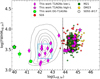 |
Fig. 1. log(FWHMHβ, br)−log(LHβ, br) parameter space for our BL AGNs (T1AGNs) and the reference samples (SDSS dr17, Shen 2016 S16, Matthews et al. 2021 M21, and Deconto-Machado et al. 2023 DM23), where the SDSS dr17 AGNs are shown with contours. We also include the three BL AGNs in metal-poor dwarf galaxies (DG-T1AGNs). The dashed line marks the threshold luminosity dividing the high- and the low-luminosity sub-samples. The actual log(LHβ, br) of SBS_0335-052E (black thick edge) is 38.3, but it was shifted to 40.0 for the sake of a tighter image layout. The azure and black rectangles mark the regions adopted to define the control samples (Sect. 4). |
As a complement to our sample, we also introduced some reference samples at lower z that were purposefully chosen in order to compare the properties of our objects. In particular, for what concerns the low-luminosity sub-sample, we chose the sources from the latest Sloan Digital Sky Survey (SDSS; York et al. 2000) quasar catalogue, whose properties are described in Wu & Shen (2022). We selected sources below z = 0.8 with reliable Hβmeasurements, by applying the quality cuts suggested in Wu & Shen (2022) (see their Sect. 4 for details).
With respect to the high-luminosity regime, a complication for finding suitable reference samples is given by the prevalence of quasars at redshift z ∼ 2 − 3, the so-called quasar epoch. At these redshifts, the Hβregion falls in the H band which is not covered by large optical surveys. For this reason, we opted for objects targeted by near-infrared (NIR) surveys. In particular, we adopted the samples described respectively in Shen (2016), Matthews et al. (2023) and Deconto-Machado et al. (2023)3. The Shen (2016) sample comprises 74 luminous quasars (Lbol = 1046.2 − 48.2erg s−1) between 1.5 < z < 3.5, observed with NIR (JHK) slit spectroscopy covering the rest-frame Hβ, Fe II and [O III] region. The catalogue described in Matthews et al. (2021) constitutes the Gemini Near Infrared Spectrograph-Distant Quasar Survey (GNIRS), containing a sample of 226 quasars between 1.5 < z < 3.5 with IR data covering the rest-frame optical/UV range. Lastly, the Deconto-Machado et al. (2023) sources are a similar sample of luminous (log(Lbol/(erg s−1)) ∼ 47.0 − 48.5) objects at 2.3 < z < 3.8, with spectral coverage in the rest-frame optical band, purposefully observed with the goal of describing the Fe II and Hβproperties at intermediate z. We also included among the luminous sources the SDSS sources falling above the luminosity threshold, although most of them cluster along the threshold line.
Lastly, alongside the main sample of low-luminosity JWST objects, we considered three extremely metal-poor dwarf galaxies hosting a type 1 AGNs, identified by the presence of broad Hα emission lines. These are SBS_0335-052E (Izotov et al. 1990), J102530.29+140207.3 and J104755.92+073951.2 (Izotov & Thuan 2008) whose properties are described below. We included these sources as tentative very local analogues of the faint JWST AGNs since, as we will show in brief below, they share a substantial set of similarities, in terms of optical lines and X-ray properties, with the high redshift sources.
To put our sources in the broader context of the emission line and accretion properties of local AGNs, in Fig. 1, we show our sample, together with the control samples on the log(FWHMHβ,br)–log(LHβ, br)4 plane. The choice of this parameters space presents several advantages. First, since the parameters describing the accretion process, such as the black hole mass and the bolometric luminosity, can be derived from these quantities (see e.g. Vestergaard & Peterson 2006; Dalla Bontà et al. 2020), we expect objects residing in the same region of this parameter space to also share comparable accretion parameters. Therefore, it is straightforward to consistently define the control samples. Secondly, since the parameter space is defined on the basis of observed quantities, the position of our sources therein is not subject to systematic uncertainties affecting thecalibrations.
For comparison with galaxies in the local Universe, we included three metal-poor dwarf galaxies that host low-luminosity type 1 AGNs (DG-T1AGNs). The identification of the AGNs in these sources has been first confirmed by the presence of a broad (FHWM > 1000 km s−1) H[[INLINE83]] emission line in Izotov & Thuan (2008). In addition, more recent observations, 15 yr after the first ones (Burke et al. 2021), confirmed the presence of the broad components in J102530.29+140207.3 and J104755.92+073951.2, thus excluding the supernovae shock scenario (Baldassare et al. 2016). Here we also added a secure detection of a broad component in the Hβprofile.
From an observational perspective, there are several similarities between the known properties of the faint JWST AGNs and DG-T1AGNs. Both these classes of objects have remarkably low NLR heavy element abundance with the highest measured oxygen abundance values in DG-T1AGNs spanning 12 + log(O/H) 7.3 and 8.0 (Izotov et al. 1999; Burke et al. 2021), and similar values have been detected in low-luminosity JWST AGNs (e.g. Harikane et al. 2023; Übler et al. 2023; Kocevski et al. 2023; Maiolino et al. 2024a). Another noticeable feature of these objects is the X-ray (by ∼1 − 2 dex) weakness with respect to the expectations of the AGNs harboured therein (Thuan et al. 2004; Simmonds et al. 2016). Additionally, there is also tentative evidence that the fraction of DG-T1AGNs exhibiting absorption features in Balmer lines is higher than what is generally found in typical SDSS local AGNs, just as reported in faint JWST AGNs (Matthee et al. 2024; Kocevski et al. 2024; Juodžbalis et al. 2024b). However, the current sample size is limited for solid conclusions. As we will show in the following Sections, and discuss more thoroughly in Sect. 6, these properties, often observed also in the faint JWST AGNs, make AGNs in metal poor dwarf galaxies an intriguing class of local analogues to compare the properties observed at remote cosmic distances.
3. Methods
In this section we describe the techniques adopted to quantify the spectral properties of the sources in our sample.
3.1. Spectral fits
To access the spectral information embedded in the JWST spectra, we performed a detailed spectroscopic analysis, focusing on a reliable determination of the Fe II and Hβproperties. To this end, we adopted a custom-made Python code, based on the IDL MPFIT package (Markwardt 2009), which takes advantage of the Levenberg-Marquardt technique (Moré 1978) to solve the least-squares problem. The main emission lines were modelled by adopting different line profiles (Gaussian, Lorentzian). In the case of the broad Hβline in quasars, we also use a broken power-law profile convolved with a Gaussian (e.g. Nagao et al. 2006), as it proves more effective in describing the asymmetry often observed in the red side of the Hβ(see e.g. Deconto-Machado et al. 2023). The kinematics of [O III] has been tied to that of the narrow Hβcomponent, and the flux ratio between the 5007 Å and the 4959 Å components was fixed to three to one (Osterbrock & Ferland 2006). With the aim of reproducing the diversity of the Fe II emission, we included several spectral templates produced within the CLOUDY environment (Ferland et al. 2013). Specifically, we ran models on a grid spanning a wide range of physical parameters in order to broadly cover the parameter space of the Fe II emission. In particular, the models span the cloud Hydrogen density (nH) range between 108 ≤ ne ≤ 1014 cm−3, photon ionising flux (ϕ) between 1017 ≤ ϕ ≤ 1023 cm−2 s−1, microturbulence velocity values vturb fixed to 0 and 100 km s−1 and solar metal abundances (e.g. Baldwin et al. 2004; Bruhweiler & Verner 2008; Panda et al. 2018). The continuum adopted is the default AGNs continuum from Mathews & Ferland (1987). These models are then convolved with a Gaussian profile (the same for all the models as they are thought to represent co-spatial emission), shifted, and weighted during the fitting process. The parameters ultimately fitted for the Fe II templates are then the velocity dispersion and the shift of the Gaussian kernel as well as the weights of each template.
Since we adopted a non-negative least square approach to perform the fit, the weights of the Fe II templates are constrained to be positive. This implies that, in the case of low signal and/or low Fe II emission, positive spikes of noise could be interpreted as iron emission, leading to an overestimate of the actual Fe II flux. In order to mitigate this issue, we also adopted a non-parametric approach to estimate the Fe II contribution in the 4434–4684 Å bump. In brief, we performed the spectral fit without the Fe II templates and focused on faithful modelling of the emission lines included in or close to this wavelength range (chiefly He Iλ4471 and He IIλ4686). We then subtracted the best-fit models of these lines from the observed spectrum and ascribed the remaining emission to Fe II. If the integrated flux estimated by this second method was < 0, or the parametric value was consistent with zero within 1σ, we marked the measurement obtained via the Fe II templates (the parametric approach) as an upper limit.
We estimated the uncertainty on the best-fit parameters by adopting a Monte Carlo approach. Specifically, we performed the fit for 100 mock spectra for each source: the flux in every spectral channel was simulated by randomising the measured flux adopting an uncorrelated Gaussian noise whose amplitude was set by the uncertainty value in that spectral channel. After fitting every mock sample, we computed the distribution of the best-fit parameters and set the uncertainty as the standard deviation of the distribution, after applying a 3σ clipping.
Examples of the spectral fits of both a low- and a high-luminosity object are shown in Fig. 2. A complete gallery of all the fits is presented in Appendix E.
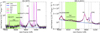 |
Fig. 2. Examples of the spectral fits of a low-luminosity (left) and a high-luminosity (right) AGN of the sample. The different components are colour-coded as stated in the legend. The uncertainty on the data is shown as a shaded area. The Fe II pseudo-continuum is highlighted in green. The vertical grey dashed lines mark the most prominent emission lines. All the spectral fits are shown in E.1. |
We report the spectral quantities of interest for the broad components, namely FWHMHβ, br, RFe and logLHβ, br5 for each object in our sample in Table A.1.
3.2. Spectral stacks
To provide an immediate term of comparison at lower redshifts for the JWST samples, we built spectral templates from the comparison samples described in Sect. 2.
Since the SDSS low-redshift sample covers a region of the adopted parameter space much wider than that spanned by our low-luminosity sample, we tailored a sample analogue to the JWST one in the FWHMHβ,br-log(LHβ, br) space. To this end, we selected a sample of SDSS AGNs in the region of the parameter space defined as [⟨log(LHβ, br)⟩ ± σLHβ, br, ⟨log(FWHMHβ, br)⟩ ± σFWHMHβ, br], with the quantities in brackets being the mean values and the respective standard deviations for the low-luminosity sub-sample. A similar approach was adopted in the high redshift regime, where we however combined the individual sub-samples individually to highlight possible differences.
We then proceeded to produce the composite spectra for the four samples by performing the following steps:
-
Each spectrum was corrected for Galactic absorption assuming the value for the colour excess E(B − V) available in the Wu & Shen (2022) catalogue according to the Schlafly & Finkbeiner 2011 extinction maps and a Fitzpatrick (1999) extinction curve. Then, the de-reddened spectra were shifted to the rest frame.
-
All the spectra in the same sample were resampled, by means of linear interpolation, onto a fixed wavelength grid. Successively all the spectra were scaled by their 5100 Å monochromatic flux, in order not to bias the stack towards the most luminous objects in each subsample.
-
The final composite spectrum was obtained by taking the median value of the flux distribution in each spectral channel. The uncertainty on the median value was evaluated as the standard deviation in each spectral channel divided by the square root of the number of sources contributing to that channel.
The same recipe was also adopted to produce the composite spectrum of the three DG-T1AGNs. The composite spectra produced as a result of this procedure, scaled by their broad Hβfluxes and continuum-subtracted are shown in Fig. 3. There are several features clearly arising from this comparison. For what concerns the Fe II emission, the low-luminosity sample at high redshift exhibits a faint Fe II emission which translates into a RFe significantly lower than the local AGNs counterparts. At the same time, the high-z quasars present a slightly fainter Fe II than the other samples, yet their RFe is on average consistent with the other reference samples. The differences in terms of the RFe ratio are more quantitatively assessed in Section 4. The lack of prominent Fe II in the low-luminosity objects can also be assessed by inspecting the fits of the composite spectra (Fig. D.1), as well as the spectral fit of each source in Fig. E.
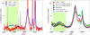 |
Fig. 3. Continuum-subtracted spectral composites of the low-luminosity (left) and high-luminosity (right) subsamples. The Hβand [O III] narrow components have been cut for visualisation purposes. In the right panel we also show the composite quasar spectra for the high-luminosity subsamples. In the case of the Deconto-Machado et al. (2023) sample we built different composite spectra for the Pop A and Pop B sub-samples, which occupy different regions of the EV1 plane. The iron bump between 4434–4684 Å (green shaded area) is evidently weaker in the JWST low-luminosity sample than in the local AGNs. Although the strength of the Fe II bump seemingly varies among the sub-samples, the RFe of the quasars at the epoch of reionisation analysed here is not significantly different from those estimated at lower z as also shown in Table 2. |
For what regards the faint-AGNs stack, we point out that the spectral fit reveals the presence of a significant6 broad (∼1000 km s−1, ΔBIC = − 116) component in the [O III] profile. This component is particularly interesting as it shows remarkable differences with respect to that observed in the SDSS control sample stacked spectrum. Firstly, this component is much fainter compared to the narrow core component than that detected in the SDSS stack. The broad-to-narrow ratio in the SDSS composite is ∼0.90, while it is about 0.11 in the low-luminosity case. Additionally, while the broad [O III] component is significantly blueshifted with respect to the core component in the SDSS stack, by ∼200 km s−1, the narrow and broad components in the faint JWST AGNs are separated by only ∼40 km s−1. Lastly, we also mention that the FWHM of the broad [O III] component is much smaller than the broad Hβ(3731 ± 133 km s−1). Notably, this finding can be viewed as a clue against the interpretation of broad lines observed in these AGNs as produced by star formation driven outflows (see e.g. Yue et al. 2024a; Kokubo & Harikane 2024). As a matter of fact, we selected this sample of AGNs only on the basis of the presence of broad lines, without any other kind of emission line diagnostic. If the mechanism producing the observed broad Hβwere star formation driven outflows, we would expect the Hβand [O III] broad components to share similar kinematics. Although the high density might lead to suppression of [O III], causing the weakness of the broad component, the broad Hβand the broad [O III] have significantly different kinematics (at 18σ). Therefore, this evidently points in the direction of a different origin for these two components.
Results of the statistical tests.
4. Results
With the aim of understanding the Fe II properties observed in our sample, in Fig. 4, we once again show the FWHMHβ, br versus LHβ, br parameter space, adding this time the RFe in colour code. For a clearer visualisation of the surface, we binned the control samples in cells containing at least 30 objects. When the JWST subsamples are compared to their control samples we observe a clear dichotomy, already foreseen in Fig. 3. The low-luminosity sample displays a RFe which results much weaker than that observed for the same regions in the parameter space for the local control sample; the only notable exceptions are JADES-209777 and XID2028, whose peculiarities will be discussed in Sect. 5. At the same time, the luminous quasars subsample is consistent, albeit with some scatter, with the expectations from the control sample at high luminosity.
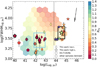 |
Fig. 4. RFe-log(FWHMHβ, br)−log(LHβ, br) plane. Specifically, he have log(FWHMHβ, br) versus log(LHβ, br) colour-coded by RFe. Objects marked with a circle represent RFe upper limits as defined in the text. The background 2D histogram is obtained by binning the control sample (with a minimum of 30 objects per bin); individual objects from JWST are colour-coded with the same scale in RFe. Due to the large number of upper limits in the low-luminosity region, we also include the values derived from the composite spectra as symbols with thicker black edges. The coloured rectangles mark the regions where the control samples were drawn. The black solid arrow marks the direction of the PCA, as described in Sect. 5.2. SBS_0335-052E (black thick edge pentagon) has been shifted for a tighter image layout. |
Quantitatively, we estimated the significance of the difference in the RFe ratios using different statistical tests to assess what is the probability that the RFe distributions of the JWST and control samples actually come from the same parent distribution as a null-hypothesis. In particular, we took advantage of the Kolmogorov-Smirnov test (KS) (Hodges 1958), the Welch’s t-test (W; Welch 1947) suited for cases of small samples with unequal variances, and the Mann-Whitney U (MW) test (Mann & Whitney 1947). Due to the reduced size of the SDSS high-luminosity sample, here we did not perform a detailed luminosity matching, but we rather choose all the sources above log(LHβ, br = 43.8, while still abiding by the FWHM cut. The results of these tests are reported in Table 2.
When the JWST samples are matched to their respective control samples in the parameter space, all the tests confirm the different behaviour already seen in Fig. 3. The difference in the RFe ratios for the low-luminosity sample is extremely significant, with p-values ≲10−6. On the other hand, the RFe measured in the JWST quasars is fully consistent with those measured at lower redshifts. In order to further strengthen these results against the possible effect of dust reddening within the BLR, we performed the same tests on a control sample chosen in order to match the average values of the de-reddened LHβ,br. Again, the difference proved extremely significant (p-value < 10−6). Lastly, we performed a further test: it has been recently pointed out that the JWST-selected AGNs show generally larger EW of Balmer lines (Maiolino et al. 2025). The smaller RFe in faint JWST AGNs could therefore be due to the larger EW Hβ, rather than to a fainter Fe II. Therefore, we performed the same tests against a sample within 0.2 dex from the mean log(EWHβ) of our faint AGNs, while still being located in the same region of the parameter space. All the tests confirmed the difference of the RFe distributions with p-values of < 2 × 10⁻⁴.
To conclude, we highlight that in the low-luminosity regime, we conservatively also included the X-ray detected AGNs JADES-209777 and XID2028. We considered the upper limits as the actual measurements estimated via the parametric fits. The exclusion of these values would make the difference even stronger.
As a more straightforward way to notice the region occupied by the JWST sources with respect to the bulk of the lower z samples, we also present two side views on the FWHMHβ, br-LHβ,br-RFe parameter space in Fig. 5. Specifically, the left panel shows RFe versus LHβ, br in (colour-coded) bins of FWHM, while the right panel shows RFe versus FWHMHβ,br in (colour-coded) bins of LHβ, br. It is clear that the low-luminosity sample exhibits systematically lower RFe than that expected for the corresponding region in the parameter space based on lower-z data.
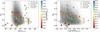 |
Fig. 5. Orthogonal sections of the log(FWHMHβ,br)−log(LHβ,br)−RFe parameter space. Specifically we have (left) RFe versus log(LHβ, br) in (colour-coded) bins of FWHMHβ,br, and (right) RFe versus FWHMHβ,br in (colour-coded) bins of log(LHβ, br). The thick-edged diamond and star represent the values derived from the composite spectra. The colour-coded lines represent the third quantity evaluated on the binned sources of the control samples. SBS_0335-052E (black thick edge pentagon) has been shifted for a tighter image layout. It is clear that, while the high-luminosity objects of the sample reside – albeit with some scatter – in the expected locus of the parameter space according to the control sample, the low-luminosity objects exhibit far lower RFe. Interestingly, two low-luminosity objects (JADES-029777 and XID2028) detach from the bulk of the faint sample, being close to the RFe expected. As we discuss further in Sect. 5.5, these are the two only faint AGNs that are X-ray detected. |
5. Possible causes of the observed differences
There is no consensus about the main drivers of the correlations involving the strength of the RFe ratio falling in the ensemble of the 4DE1.
It is generally thought that the RFe-FWHMHβ,br anti-correlation results from the combined effect of the accretion rate and inclination of the line of sight with respect to the axis of the accretion disc powering the AGNs. Yet, it is unlikely that the λEdd is per se the main driver of the 4DE1 correlation. The λEdd increases perpendicularly to the main sequence, and objects with low Eddington ratios produce very different RFe ratios. The same spread in terms of RFe is observed in samples allegedly made of sources accreting at high-Eddington ratios such as the SEAMBH sample (see e.g. Du et al. 2018). Also, from a theoretical perspective, the inclusion of a physically motivated warm X-ray corona has been observed to loosen the dependence of the RFe on the λEdd (Panda et al. 2019a).
Lastly, we must bear in mind that both the FWHMHβ,br and the Eddington ratio are easy to estimate parameters, useful when it comes to roughly describing the accretion properties of our sample, but they are not the physical quantities ultimately governing the micro-physics of Fe II and Hβemissivity. Their effect on the RFe ratio comes more subtly in the form, for instance, of a dependence of the RFe on the spectral energy distribution (SED), which, in turn depends on the accretion properties of the AGNs (Panda et al. 2019a, 2019b; Sarkar et al. 2021).
In this section, we present a series of tests aiming at exploring the possible drivers of the observed properties, in both our sample and the reference samples.
5.1. Examining whether we are probing an extreme tail of the 4DE1
Within the 4DE1 set of correlations, it is well known that objects with stronger RFe exhibit weaker [O III] emission lines and vice-versa (Boroson & Green 1992). Since our faint AGNs show on average strong [O III] emission (the median value is ∼255 Å), it is therefore legitimate to question whether the RFe weakness detected in these sources might be interpreted as the high-EW[O III] and low-RFe end of the eigenvector 1. We explored this possibility and presented several arguments against thisinterpretation.
Firstly, we note that the faint JWST AGNs are not consistent with the expectations for local (i.e. SDSS) sources in the same region of the log(EW[O III])–log(RFe) plane. This can be seen in Fig. 6. There we highlight in pink the local sources -this time not selected from the log(FWHMHβ,br)−log(LHβ,br) control sample- within 0.2 dex from the mean value of the JWST low-luminosity sources. We tested whether the RFe estimated from the JWST and the SDSS EW[O III]-matched sources could be compatible with coming from the same parent distribution, adopting the same statistical tests described in Sect. 4. The RFe distribution for the JWST sources resulted significantly different (at ≳95% confidence level, depending on the test; see Table 2) from the SDSS one. Here we also note that we made the very conservative assumption of considering the upper limits as actual measurements7. In Fig. 6 we also show that the average RFe values for the faint JWST sources are far below (∼2.4σ) the best-fit relation for the SDSS full sample. There we estimated the average RFe in multiple ways: including the upper limits as actual measurements (maroon), extracting the non-detected values from a uniform distribution between the SDSS lowest 1st percentile and the upper limits (red), and using the value derived from the spectral fit of the stack (magenta).
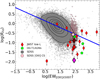 |
Fig. 6. log(EW[O III])–log(RFe) section of the 4DE1. The pink dots mark the SDSS objects selected as a control sample. The blue line highlights the best linear fit to the SDSS data. The thick-edged diamonds represent the average values for the faint JWST AGNs as described in the text. |
Furthermore, other arguments can be brought against the faint JWST sources fitting within the 4DE1 framework, which are the average Eddington ratio and the inclination. The Eddington ratio, albeit the already mentioned caveats, is generally observed to correlate, with RFe (e.g. Shen & Ho 2014). These sources exhibit, on average, the same Eddington ratio as their low-z counterparts, having ⟨λEdd⟩∼0.14 (⟨λEdd⟩SDSS ∼ 0.11) if we adopt the Vestergaard & Peterson (2006) calibration for the black hole mass and the Richards et al. (2006) for the bolometric luminosity. Although the validity of the local calibrations in these so different environments is questionable, the resulting RFe is far lower than the expectations. The other mechanism classically invoked to explain the 4DE1 trends is the inclination of the line of sight. Objects with large [O III] are thought to be observed under large viewing angles (e.g. Risaliti et al. 2011Risaliti et al. 2011; Bisogni et al. 2017), while a more face-on inclination decreases the [O III] EW while increasing RFe. However, the large fraction of JWST low-luminosity objects with large (EW[O III] ≳100 Å) does not seem reconcilable with the local one (∼4% in Fig. 6). At the same time, the inclination hypothesis to explain the large [O III] would leave room for the other, perhaps even more striking question that considers where we should find all the low-inclination, low EW[O III] sources at these redshifts.
Lastly, we mention that all the considerations made so far subsumed the AGNs nature of the [O III] emission. This could be not the case, as for these sources a significant fraction of the [O III] emission could be ascribable to star formation. Indeed, star-forming galaxies and the AGNs discovered at these redshifts overlap in the classical BPT diagrams (see e.g. Maiolino et al. 2024a; Kocevski et al. 2023; Harikane et al. 2023). Therefore, the EWs computed here would only be an upper limit to those actually coming from the AGNs. Disentangling the AGNs contribution from the star-formation would result in a shift leftwards of the average [O III] values in Fig. 6. This would lead to an even stronger inconsistency with the SDSS 4DE1.
5.2. Accretion parameters
The accretion parameters (i.e. the black hole mass and the accretion rate, or its closely related observable, the luminosity) are thought to ultimately rule, with a few other parameters, the shape and the emissivity of the accretion disc in AGNs. These quantities are expected to be, therefore, the strongest drivers in the changes of the AGNs SED, mainly responsible for the photoionisation in these sources. Hence, an obvious point is to assess whether the observed difference in RFe could be ascribed to changes in one or both of these parameters (see e.g. Panda & Marziani 2023).
Nonetheless, there are some complications: the first is the fact that the evaluation of the MBH comes with a significant systematic uncertainty due to single-epoch calibrations (between 0.4–0.5 dex, see e.g. Shen 2013; Dalla Bontà et al. 2020). In this work, we adhered to the Vestergaard & Peterson (2006) prescription, for the black hole mass estimation and the Richards et al. (2006) for the bolometric luminosity, for consistency with the control sample. All the values derived for the sample are listed in Table B.1. In addition to the large systematic uncertainty, the applicability of such calibrations to the class of low-luminosity JWST AGNs where, for instance the BLR covering factor could be systematically different (e.g. Maiolino et al. 2025), is far from obvious.
Moreover, there is not a univocal well-defined relation between the RFe and any of the accretion parameters, but the λEdd which, however, suffers by a large systematic uncertainty deriving from the combination of that on the black hole mass and on the bolometric luminosity. In the effort to understand the evolution of the RFe within our parameter space, we took advantage of a partial correlation analysis (PCA). This technique allows us to estimate the correlation between two quantities (in our case the RFe and the main axes of the parameter space) while holding fixed any other components.
In particular, given the three quantities (A, B, and C), the partial correlation coefficient between A and B at fixed C can be expressed as:
 (1)
(1)
where ρAB ∣ C denotes the Spearman rank correlation index between A and B, while keeping C constant. We also note that a monotonic trend is a requirement for the PCA to provide meaningful results, and this is mostly true as the RFe tends to increase with decreasing FWHMHβ,br and increasing LHβ,br.
We used the PCA values to define a gradient arrow in Fig. 4, whose inclination is defined as:
 (2)
(2)
The more the arrow is aligned with an axis, the stronger is the correlation with that quantity. The correlation with the FWHMHβ,br is significantly stronger than with the LHβ,br, yet both of them yield low, yet significant, partial correlation coefficients ( with p-value < 10−6 and
  with p-value < 10−6). At fixed LHβ,br, the increase in FWHMHβ can be readily interpreted as an increase in MBH, as a consequence of the H[[INLINE212]] virial relation (see e.g. Dalla Bontà et al. 2020 and references therein), a finding similar to that in Wildy et al. (2019). At the same time, LHβ,br is tightly related to the 5100 Å luminosity (see e.g. Yee 1980; Kaspi et al. 2005; Dalla Bontà et al. 2020) which in turn is a good proxy to the bolometric luminosity (Richards et al. 2006). Yet, none of these two parameters seems to be a strong driver of the observed changes in RFe. Additionally, we recall that the difference evaluated in Section 4 has been computed between the JWST low-luminosity objects and their local counterparts in the parameter space, which is tightly related to the accretion parameters. Therefore, we do not expect either the black hole mass nor the luminosity to be driving the observed difference, under the non-trivial assumption that the local calibrations apply also for this class of AGNs. The same consideration applies to the Eddington ratio as well.
5.3. Effects of metallicity
A trivial factor which could be responsible for the weakness of the Fe II bump is the metallicity. Here, we explore what we can infer about the gas-phase metallicity for the low-luminosity sources by employing line diagnostic ratios.
Extensive work based on CLOUDY simulations showed that it is possible to reproduce the diversity in the optical RFe of the low-z SDSS sample, while allowing for a super-solar metallicity [1 Z⊙–10 Z⊙] and keeping the other BLR parameters, such as the density and the column density, within the typical range (Panda et al. 2018). However, there is evidence for the faint objects in this early stages of the Universe not to have reached the chemical maturity observed in more local sources, at least in the NLR (Curti et al. 2023; Isobe et al. 2023; Maiolino et al. 2024a; Übler et al. 2023, 2024; Kocevski et al. 2024). This points in the direction of low metallicity as a possible driver of the low RFe ratios observed in our sample.
5.3.1. Preliminary considerations
The most straightforward way to estimate the metallicity of the BLR gas in these sources would be to employ high ionisation line ratios such as N V/C IV or (Si IV + O IV)/C IV (see e.g. Lai et al. 2022 and references therein). Unfortunately, this wavelength range is not accessible within our spectra. Alternatively, we could infer the metallicity from the readily available rest-optical lines in the NLR, but translating this measurement into a BLR metallicity would require a model of the chemical enrichment and of the interplay between these two spatially different regions at these early cosmic epochs.
From an observational point of view, it is well known that the BLR and NLR metallicities are linked, with the former reaching generally higher metallicity (Z ≳ Z⊙; e.g. Wang et al. 2022) at early cosmic epochs. However, this link between the NLR and BLR metallicities implies that even if we managed to get reliable estimates of the NLR metallicity for the low-luminosity objects, these would only set a lower limit to the corresponding BLR metallicity.
In addition, estimating the metallicity of the NLR in AGNs is not a well-established procedure (see e.g. Dors et al. 2020a for a compilation of the few attempts made in this direction) and efforts in this field have been mainly directed towards type 2 AGNs (Thomas et al. 2019; Dors et al. 2020b; Li et al. 2024). An example of complications in estimating the AGNs metallicity is the higher fraction of O3+ (whose corresponding transitions are undetectable in the optical range). This is associated with the harder AGNs continuum and the effect of temperature inhomogeneities in the NLRs (Riffel et al. 2021).
For our sample, the most direct way to estimate the NLR metallicity is via the electron temperature method (Smith 1975), which is based on the use of the [O III] λ4363 auroral line. Unfortunately, this line is robustly detected in only 6 out of 14 low-luminosity AGNs. In comparison, strong-line methods would usually require detection of low ionisation lines such as [N II] λλ6548,6584, which are outside of the wavelength coverage for most of the sample, or barely detectable as outshone by the broad H[[INLINE222]]. We also recall that it is quite challenging to detect the [O III] λ4363 line in local type 1 AGNs to make comparisons with the JWST results, as it is generally faint and not easy to deblend from the narrow and broad H[[INLINE224]] and the Fe II pseudo-continuum (Baskin & Laor 2005). This leads to the additional complication of having a comparison sample (the SDSS local AGNs catalogue) where metallicity measurements would be questionable and biased towards high [O III] λ4363 emitters. In addition, it is well known that the metallicity of H II regions and star-forming galaxies, directly estimated via this method, are systematically lower than those produced adopting calibrations from photoionisation modelling by 0.1–0.4 dex (see e.g. Kennicutt et al. 2003; Dors & Copetti 2005; López-Sánchez et al. 2007; Kewley & Ellison 2008; Marconi et al. 2024). This difference is even exacerbated in the case of AGNs with the oxygen abundance being underestimated on average by 0.6–0.8 dex (Dors et al. 2015, 2020a).
Lastly, we note that the oxygen abundance estimated via the Te method or other calibrations (e.g. Storchi-Bergmann et al. 1998; Castro et al. 2017) does not necessarily trace the actual iron abundance, unless a chemical enrichment model is assumed. Indeed, high-redshift objects have been observed to display gas-phase oxygen abundances consistent with those observed locally (e.g. Arellano-Córdova et al. 2022; Jones et al. 2023). This follows as a consequence of the enrichment by core-collapse supernovae, while the total Fe abundance is expected to be significantly lower, having this element a delayed enrichment contribution from type Ia supernovae. An additional complication is the fact that Fe is heavily depleted onto dust grains (see e.g. Jenkins 2009; Shields et al. 2010). Although, within the standard evolutionary picture, the effect of depletion onto dust grains in the redshift range spanned by our sources is not expected to be a crucial channel to suppress the Fe II emission, as it might happen at lower redshift (Shields et al. 2010), more detailed studies are definitely needed to assess this possibility.
5.3.2. Oxygen abundance
Notwithstanding all these considerations, for 6 out of 14 objects we detected [O III] λ4363 with a signal-to-noise ratio of S/N ≥ 3. Assuming Gaussian uncorrelated noise, and the redshift of each source being well determined, the 1-tailed probability of a false 3-sigma detection of [O III] λ4363 is ∼10−4. Supposing, in the worst case scenario, that the [O III] λ4363 line were actually absent in all sources, the joint probability of having 6 or more detections only due to positive statistical fluctuations would be ≃3 × 10⁻¹⁴. In the following, we assume all detections to be real and we proceed with an estimation of the gas-phase oxygen abundance.
We derived the electron temperature (Te) using the PYNEBgetTemDen routine (Luridiana et al. 2015). In all these objects, we could access the typical optical density indicator [O II] λλ3726,3729, but could not disentangle the doublet. To compensate for this, we computed the electron temperature using an equispaced grid of densities from 101 cm−3 to 105 cm−3. For each density value we evaluated the corresponding temperature of the high ionisation region (t3) using the ratio between the [O III] λ5007 and the [O III] λ4363 emission lines (the O33 ratio) using the getTemDen routine8. Finally, we computed the oxygen abundances employing the PYNEBgetIonAbundance routine. The uncertainty associated with the abundance measurements was derived as the 16th − 84th semi-interpercentile range of the abundance distribution obtained by varying the density.
We estimated the electron temperature for the low ionisation zone (t2), adopting the relation t2−1 = 0.693 t3−1 + 0.2819 (see e.g. Dors et al. 2020a). Additionally, we corrected the total oxygen abundance for the unobserved ions adopting an average ionic correction factor (ICF) equal to the mean value of those measured in the Seyfert 2 sample described in Dors et al. (2020b), that is ICF(O2+) = 1.21. For all the objects, this procedure yielded reasonable results with sub-solar oxygen abundances ranging between Z = 12 + log (O/H) = 7.7 − 8.0 and electron temperatures between 15 000 K and 25 000 K. The values obtained via this procedure are reported alongside other narrow emission line ratios for the low-luminosity sample in Table A.1, where we also present the values derived for the DG-T1AGNs.
With the aim of comparing the NL properties between all the JWST low-luminosity sources and their local counterparts, in Fig. 7 we show RFe against the [O III]/H[[INLINE249]] ratio, while in colour-code we highlight the O32 ratio for the comparison sample. It is well known that there are several parametersinfluencing the [O III]/H[[INLINE250]], namely the ionisation parameter, the metallicity, the shape of the ionising continuum, and the density (e.g. Veilleux & Osterbrock 1987). The dependence on all these parameters makes this ratio a suitable tool for interpreting observations of the nebular emission from active and inactive galaxies. In our case, the selection of a homogeneous control sample in terms of black hole mass and luminosity helps in narrowing down the parameter space. Indeed, assuming that the optical/UV region of the SED is dominated by an accretion disc, we do not expect the ionising continua to be dramatically different as the average accretion parameters are, by sample construction, close. In more quantitative terms, the difference in average log(MBH) and log(Lbol) between the local sample and the JWST low-luminosity one amounts respectively to 0.15 and 0.19 dex, which is fairly close or even lower than the typical systematic uncertainty 0.4 dex and 0.3 dex. We therefore expect the shape of the continuum to be comparable between these two samples as well as within the local sample itself. Similar considerations concerning how the shape of the SED should be limited by construction, apply to the diversity along the RFe axis in Fig. 7.
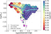 |
Fig. 7. Distributions of the SDSS analogues and our JWST faint AGNs sample in the log([O III]/H[[INLINE259]]])-log(RFe) plane with the O32 ratio colour-coded (except for the faint AGNs where the [O II] was not measured). White contours show the distribution of SDSS AGNs. The diamond with thicker black edges represents the value derived from the low-luminosity composite spectrum. Alongside the main anti-correlation, a secondary branch of SDSS objects detaches (the dashed lines guide the eye along the two branches), which still shares O32 values similar to those of the main trend. Notably, the JWST low-luminosity sources follow this steeper anti-correlation trail, likely driven by low metallicity as explained in the text. |
Additional information can be gained by employing the O32 ratio, colour-coded in Fig. 7 for the SDSS control sample, which serves as a useful proxy for the ionisation parameter. In our low-luminosity sample the [O II] λλ3726,3728 doublet was reliably detected, albeit unresolved, in only a handful of JWST objects, while it was clearly measured in all the DG-T1AGNs. For this reason, we only colour-code accordingly these few sources in Fig. 7.
It is thus interesting to observe that, from the main anti-correlation trend between RFe and [O III]/H[[INLINE254]], which is basically a shallower version of the well-known RFe-[O III]anti-correlation, an even steeper anti-correlation branch detaches (see the dashed lines in Fig. 7). Notably, the JWST low-luminosity objects sit nicely on this secondary branch. The nature of this secondary branch is not clear, but a speculative hypothesis is that this sample might represent a low metallicity trail. This interpretation seems favoured by the fact that the trail detaching at low values of RFe displays similar O32 values to those following the main trend. The same roughly holds for the faint AGNs for which this ratio was estimated. Indeed, once the shape of the ionising SED and the ionisation parameter (O32) are roughly fixed, [O III]/H[[INLINE255]] would increase with increasing metallicity at low metallicities and decrease with increasing metallicities at high metallicities (Groves et al. 2006; Curti et al. 2016; Dors et al. 2015)10. Thus, we can interpret the lower left branch occupied by the low-luminosity sample as having lower metallicities compared to the SDSS sources at similar ionisation parameters, even though we do not have access to O32 for all of the low-luminosity sources.
If this scenario proved consistent, the weakness of the RFe in these sources could well be an effect of the reduced metal content, as this seems also the case for the three DG-T1AGNs, whose metallicities are notoriously low. Still, we caution that the metallicities and ionisation parameters we infer from narrow lines only reflect the properties of NLRs. Indeed, BLRs can have chemical abundances enriched earlier than NLRs and their ionisation parameters are not necessarily connected to each other. Regardless, confirmations of metal-poor NLRs in low-luminosity sources would have room for the existence of metal-poor BLRs. In contrast, the more metal-rich NLRs in SDSS sources would likely indicate even more metal-rich BLRs. To understand more quantitatively what might be driving the difference in RFe, we took advantage of theoretical photoionisation models to predict RFe under different physical conditions in the next section.
5.4. Photoionisation models
5.4.1. Model set-up
To better understand the difference in RFe between the low-z SDSS sample and the high-z JWST sample, we used theoretical photoionisation models computed with CLOUDY (v17.03, Ferland et al. 2017). In the computation of the models, we turned on all levels available for Fe+ with atomic data sets implemented by Sarkar et al. (2021), from Bautista et al. (2015), Tayal & Zatsarinny (2018), and Smyth et al. (2019). The theoretical computation of the strength of Fe II has been investigated by many previous works, which showed that RFe broadly depends on parameters such as the Fe abundance, the gas volume density, the gas column density, the ionising photon flux, the shape of the ionising SED, and the microturbulent velocity (e.g. Baldwin et al. 2004; Ferland et al. 2009; Panda et al. 2018, 2020; Panda 2021; Temple et al. 2020; Sarkar et al. 2021). For the purposes of this work, we make and justify the following assumptions and simplifications during photoionisation modelling, with the model parameters summarised in Table 3.
Input parameters for CLOUDY photoionisation models.
First, we restrict the comparison between the low-z and high-z samples to a region within the observed parameter space with similar broad Hβluminosities and FWHM (see Fig. 1). Based on this selection criterion, we assume both samples of AGNs share comparable accretion properties and thus do not differ significantly in their ionising SED produced by the accretion discs. Specifically, we start our calculation by assuming the shape of the SED to follow the functional form
 (3)
(3)
where, by default, we set the temperature of the cutoff of the “big blue bump” component to TBB = 106 K, the UV-to-X-ray slope to αox = −1.4 (by adjusting a in the equation above), the UV slope to αuv = −0.5, and the X-ray slope to αx = −1.0. It is worth noting that this assumption might not hold over the full energy range of the SED, as the majority of the JWST identified AGNs in our sample is clearly X-ray weak. Recently, Maiolino et al. (2025) suggested two potential reasons for the lack of hard X-ray detections in early AGNs, one being the intrinsic lack of the hard X-ray component due to the missing hot corona, the other being the presence of Compton-thick and dust-free clouds within the BLRs. The former scenario is also proposed by Lambrides et al. (2024), who suggest αox < −1.8 for many JWST-selected BL AGNs and ascribe the steepening of the UV-X-ray spectrum to super-Eddington accretion. To take into account these effects, we perform two additional tests by computing models with suppressed non-thermal X-ray components and models with Compton-thick clouds to X-ray emission, which we describe later in this section. We also note that Equation (3) is an analytical approximation to realistic AGNs SEDs. To check whether realistic AGNs SEDs produce any significantly different results, we use AGNs SEDs computed from multiwavelength observations by Jin et al. (2012, 2017) covering sub-Eddington to super-Eddington regimes and describe the results in Appendix F. Overall, our conclusions remain largely unchanged with the realistic SEDs.
Second, we assume a fixed gas density and a fixed microturbulence velocity. Specifically, we adopted a hydrogen density of nH = 1011 cm−3, a value encompassed by those explored in many previous Fe II modelling works and is typical for BLR regions (e.g., Joly 1987; Netzer 1990; Collin & Joly 2000; Sigut & Pradhan 2003; Baldwin et al. 2004; Ferland et al. 2009; Panda et al. 2018; Sarkar et al. 2021). While there is evidence that the ISM density in galaxies is gradually increasing with redshift, there is neither observational evidence nor theoretical expectation that a similar evolution should exist in the BLR surrounding supermassive black holes. Systematic studies about the evolution of the BL strength with redshift point in the direction of a lack of evolution with cosmic time (Croom et al. 2002; Stepney et al. 2023). The same consideration applies to the ionisation parameter, which is observed to increase with redshift in the ISM, but its redshift evolution within BLRs is not clear and its value strongly depends on the geometry. We further discuss the effect of the ionisation parameter together with that of the metallicity later in this section. Regardless, we check the effect of the density variation by computing models with nH = 1010 cm−3 and nH = 1012 cm−3, respectively. In general, at the lower density, RFe is enhanced at low ionisation parameters but suppressed at high ionisation parameters. At the high density, the opposite effect of the ionisation parameter on RFe is seen. This can be understood as the fact that Fe II is optimally emitted by clouds with certain combinations of densities and ionising fluxes (e.g. Baldwin et al. 2004), and the latter is simply the product of the ionisation parameter and the density. In Appendix G, we further discuss the effect of density variations.
The microturbulence is usually included in the photoionisation modelling of BLRs as a source for producing large Doppler broadening of line profiles within the photoionisation mean free path for line productions. The microturbulence strengthens the continuum pumping and line fluorescence that produce Fe II emission, and reduces the optical depths of Fe II lines (e.g. Netzer & Wills 1983; Baldwin et al. 2004). Although the origin of the microturbulence in BLRs remains debated (see Sect. 8.1 in Baldwin et al. 2004 for a review of possible mechanisms), it is generally agreed among the previous modelling works that a microturbulent velocity of at least vturb = 100 km s−1 is needed to correctly predict Fe II emission (Panda et al. 2019a), which is also what we adopted in our models. Lower values for the microturbulence (e.g. 20 km s−1) have been show to provide similar RFe values, but requiring lower cloud metallicity (Panda 2021). One potential way to connect the microturbulence to the other peculiar features of this sample, in particular the X-ray weakness, is to consider the magneto-hydrodynamic (MHD) wave explanation, where the microturbulence comes from non-dissipative waves generated bymagnetic fields (Bottorff & Ferland 2000). If the hot corona producing the hard X-ray emission (E ≳ 2 keV) is missing in these low-luminosity AGNs due to the absence of the magnetic field lifting the corona from the accretion disk, it might be reasonable that the microturbulence is also suppressed and even vanishing in these early AGNs, leading to reduced emergent Fe II emission. The issue with this explanation is that the reason for the vanishing magnetic fields is not clear and it is also not clear whether the microturbulence should rise from the MHD waves.
We note that it is still possible that the density and microturbulence play a role in producing the difference in RFe we observed. Our choice of not varying these parameters is mainly motivated by the fact that their redshift evolution is neither expected nor observed. The main parameters we inspect are the metallicity (or, more precisely, the iron abundance), the power-law X-ray component of the SED, and the hydrogen column density. Although previous works on BLR metallicities of bright quasars suggest fast chemical evolution within BLRs (e.g. Dietrich et al. 2003a; Maiolino et al. 2003; Wang et al. 2022), our sample mainly consists of lower luminosity type 1 AGNs and it is not unreasonable to speculate they are more metal-poor compared to the local AGNs. Checking the effect of the X-ray component and the hydrogen column density, as we have explained, is motivated by the fact that the JWST identified type 1 AGNs are mostly X-ray weak. One potential explanation is the lack of hot coronae in these AGNs, meaning the absence of the power-law X-ray component in their SEDs, an occurrence verified for instance in Ricci et al. (2020) to explain the drastic transformation of the X-ray properties following a changing-look event. The other potential explanation is the presence of Compton-thick (NH ≳ 1.5 × 1024 cm−2) and dust-free clouds within their BLRs. While such properties might not be uncommon for line-emitting clouds within BLRs (Netzer 2009), to significantly obscureX-ray emission, they need to have a large covering fraction near unity. This might also explain the high EWs of broad Hα in early AGNs (Maiolino et al. 2024a; Wang et al. 2024) and could be caused by the metal-poor environments and the consequent ineffective removal of dense gas through radiation pressure.
To check the effect of including clouds that are Compton-thick to the X-ray, we computed additional models with NH = 1025 cm−2 (compared to NH = 1024 cm−2 by default). We note that the typical column density adopted by previous works to investigate low-ionisation lines such as Fe II and Ca II from the BLR is NH = 1024 cm−2, although NH ≳ 1024.5 cm−2 helps to reproduce Fe II and Ca II emission of some AGNs (e.g. Ferland et al. 2009; Panda et al. 2020; Panda 2021). At NH = 1025 cm−2, the cloud becomes optically thick to X-ray photons via Compton scattering and thus radiative transfer effects, which are not treated precisely in CLOUDY, become important. Still, optical photons are only effectively scattered by free electrons, and the scattering optical depths for this process remain τe < 1 in our models. We also check models with an intermediate column density of NH = 1024.5 cm−2 (not shown) as did by Panda et al. (2020), and our conclusions remain largely unaltered.
Finally, the intrinsic sizes of individual BLR clouds (given by NH/nH) could set an upper limit on the plausible choice of NH (Ferland & Persson 1989; Panda 2021). There are only a few observational constraints on the sizes of BLR clouds in local AGNs. For example, Maiolino et al. (2010) used occultation of X-ray emission to estimate a lower limit of 3 × 1011 cm for the obscuring BLR cloud in NGC 1365. Peterson (2006), on the other hand, used the BLR covering factor and line luminosities derived from the observations of NGC 5548 to indirectly infer a cloud size of roughly 1013 cm. The latter would be incompatible with NH = 1025 cm−2 and nH = 1011 cm−3 we set in this alternative simulation framework (although one could further increase nH to match the cloud size). However, we note that there are loose observational constraints on the BLR cloud size of X-ray weak AGNs similar to JWST sources, and our goal here is to test if the Compton-thick scenario leads to any noticeable difference in our model results.
5.4.2. Comparison between models and observations
In Fig. 8, we compare our CLOUDY model predictions with RFe measured in our sample. Specifically, from our sample, we plot the mean RFe of the whole JWST sample, the X-ray weak JWST sample, and the SDSS analogues matched in Hβluminosities and FWHM, together with the corresponding 1σ uncertainties. The mean RFe of the SDSS sample is roughly 3.5 times that of the whole JWST sample, which is roughly 1.6 times that of the X-ray weak JWST sample. We plot the model predicted RFe as a function of the metallicity and the ionisation parameter. At fixed ionisation parameters, RFe generally increases with increasing metallicities. Although Fe II transitions are important cooling channels in the partially ionised zones within the BLR clouds, meaning their strengths are largely determined by the heating and cooling equilibrium rather than the Fe abundance, this effect is stronger for the UV Fe II transitions, while the optical Fe II transitions have a stronger metallicity dependence (Shields et al. 2010). At fixed metallicity, on the other hand, RFe does not exhibit a strong dependence on the ionisation parameter for log U > −2.5 and only starts to significantly increase with decreasing ionisation parameters for log U < −2.5. At low ionisation parameters, the intensity of Hβdrops significantly due to the drop in the ionisation rate. In contrast, due to the low ionisation potential of Fe, the intensity of Fe II from the partially ionised zone decreases more gradually than the Hβ. If we only focus on the high ionisation parameter branch, the mean RFe of the SDSS sample is consistent with Z/Z⊙ ≳ 2, and the mean RFe of the JWST sample can be explained by 0.1 ≲ Z/Z⊙ ≲ 0.5. In comparison, we mark the potential range of the NLR metallicities for the JWST sample with the shaded region. We note that the BLR metallicities could be well above the NLR metallicities, and the abundance ratio of Fe/O could also be different. Regardless, from these models, the metallicity difference appears as a plausible explanation for the much lower RFe in the JWST sample.
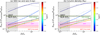 |
Fig. 8. Comparisons between RFe predicted by photoionisation models with different input parameters and RFe measured in our sample. In each panel, the green line indicates the mean RFe found in the SDSS sample that matches the JWST sample in terms of Hβluminosities and FWHM; the magenta shaded region corresponds to the value found in the JWST sample; the red shaded region corresponds to the value found in the JWST sample excluding sources with X-ray detections, which also happen to be the strongest Fe II emitters among the faint AGNs. The grey shaded region indicates the plausible range of metallicities in the NLRs of the JWST sources based on the Te method for a subset of the JWST sample. Photoionsation model predictions are plotted as a function of the metallicity, Z/Z⊙, and are colour-coded by the ionisation parameter. Left: solid lines and dashed lines correspond to models with and without a hard X-ray component representing the hot corona contribution to the SED, respectively, Right: solid lines and dashed lines correspond to models having NH = 1024 cm−2 and NH = 1025 cm−2, respectively. |
On the left panel of Fig. 8, we simulate the effect of an intrinsic X-ray weakness by virtually removing the corona. We achieved this by computing a set of models with αox = −5, which effectively makes the power-law X-ray component contributed by the hot corona negligible compared to the emission from the accretion disc (see Appendix F). The resulting models are plotted as dashed lines, which do not predict very different RFe compared to our fiducial models with αox = −1.4 at given metallicities and ionisation parameters. This is expected as the hard X-ray component should generally contribute little to the ionisation as well as heating of the gas, and consequently RFe. In addition, compared to the accretion disc emission, the hot corona contributes little to the total soft X-ray emission that is responsible for creating the partially ionised zone where Fe II originates from. We emphasise again that we assume no significant difference in the shape of the accretion disc emission between the SDSS analogues and low-luminosity sources, given their accretion parameters are empirically constrained to be similar by their broad Hβluminosities and FWHM. On the right panel of Fig. 8, we check the effect of thicker BLR clouds with larger column densities reaching NH = 1025 cm−2. As expected, increasing the column density increases RFe. This is because Hβis mainly produced by the ionised layer of the clouds, whereas Fe II becomes the major coolant at large cloud depths, and thus increasing the cloud depths tends to boost RFe. However, this trend is opposite to what is observed, that is, a decrease in RFe at early times. Again, we caution that the radiative transfer of X-ray photons are not rigorously treated for these Compton-thick models, although the clouds remain optically thin in terms of electron scattering for optical photons including optical Fe II photons.
To summarise, neither the hot corona emission nor the column density seems to cause the observed difference in RFe. The metallicity is likely the most important factor governing the RFe in our sample, consistent with our interpretations based on RFe versus NL ratios in Fig. 7. These analyses point towards the picture where, unlike luminous quasars at early times, the low-luminosity AGNs in our sample have less chemically evolved BLRs or, at least, less Fe-enriched BLRs. We further discuss the implications for the chemical evolution of these systems in Section 6.
5.5. An X-ray perspective
The low-luminosity AGNs population discovered by JWST is prevalently undetected in the X-ray surveys (Yue et al. 2024a; Maiolino et al. 2025) with the detection efficiency being below the percent level (see e.g. Kocevski et al. 2024). Our sample makes no exception, with all (but two) of the low luminosity sources being undetected in the X-rays in their respective fields. This also applies for the three newly discovered RUBIES objects where no X-ray counterpart was found in the 800 ks of the Chandra Aegis-X Deep survey catalogue (Nandra et al. 2015). The only two non-quasar sources which escape this picture are XID2028 and JADES-209777, both of them reliably X-ray detected as reported in Brusa et al. (2010) and Juodžbalis et al. (2025). Intriguingly, these sources are the objects with the highest RFe below the quasar luminosity regime (respectively RFe = 1.10 and RFe = 0.44), and in line or even above the RFe expectations for the local sources in the corresponding region of the parameter space (see the colour-code in Fig. 4). Although it is certainly risky to draw conclusions based on such a small number statistics, it is interesting to notice that the only two X-ray detected sources of the sample are also those on the high end of the RFe distribution for the JWST low-luminosity objects.
From a theoretical perspective, it is not straightforward to link the X-ray properties with the RFe strength. As we showed in Sect. 5.4, the intensity of the optical iron does not strongly correlate with the hard X-rays component. This is due to the fact that the Fe II is mostly produced at optical depths where the heating and the ionisation are due to lower energy soft X-ray photons rather than hard X-ray photons. This prediction is confirmed by observations, whereby RFe does seem to positively correlate with the so-called soft excess, i.e. the low-energy (≲0.5 keV) extrapolation of the hard X-ray power law (Wilkes et al. 1987; Wang et al. 1996; Shastri et al. 1993). This broadly agrees with the findings on NL Seyfert 1 galaxies, whose X-ray spectra on average steep, being generally stronger optical iron emitters. Here we mention two possible scenarios to link X-ray and RFe weaknesses. In the first case, the accretion parameters characterising the local and the high-z sources are systematically disparate because of different MBH and Lbol calibrations between these two populations. Therefore, these classes of sources have intrinsically distinct soft X-ray SEDs that lead to the observed RFe difference (see for instance Panda et al. 2019a). Alternatively, it is possible that the low metallicity of the BLR clouds causes both the X-ray and the RFe weakness. We already showed in Sect. 5.4 that the RFe observed in the faint JWST AGNs are consistent with metal-poor BLR. Qualitatively, we can speculate that this effect might also lead to the BLR clouds lingering close to the innermost AGNs engine because of the low effective radiation pressure. Therefore, the reduced metal content removes the metal-line transitions, which help reaching the dynamical equilibrium, from BLR clouds and causing them to linger closer to the nucleus.
We also highlight that both these X-ray detected sources have substantially lower redshifts than the bulk of the low luminosity sample (⟨z⟩ = 6.34), in particular z = 1.59 for XID2028 and z = 3.71 for JADES-209777. The only other object at a somewhat lower redshift from the bulk of the redshift distribution of the low luminosity sample is JADES-028074 (Juodžbalis et al. 2024b) at z = 2.26. This object is of utmost interest as it encapsulates some of the typical properties of the faint JWST AGNs, such as the X-ray (and radio) weakness, the lack of ionised outflows, and hereby we also add the RFe weakness, at the same time showing correlated absorptions in the Hβ, H[[INLINE328]] and He I. Within an evolutionary framework, sources akin to JADES-028074, might be experiencing the transitioning phase between an AGN with the characteristics of the faint JWST AGNs and those of Seyfert 1 AGNs observed at lower z exemplified by JADES-209777 and XID2028. In a wider perspective, the significant fraction of JWST-detected AGNs with absorption features in the broad lines (Matthee et al. 2024; Kocevski et al. 2024; Wang et al. 2024; Juodžbalis et al. 2024b; Taylor et al. 2024; Maiolino et al. 2025) could be experiencing the ‘blow-out’ phase bridging between the obscured and unobscured stages of the AGNs cycle (Hickox & Alexander 2018). Yet, the outflow velocities reported in this case are significantly lower than those seen in the nuclear region of quasars measured from broad absorption lines or in X-ray spectra (a few hundred versus tens of thousands km s−1).
6. Discussion
The first years of JWST observations have revolutionised our understanding of the high-redshift Universe, in particular, by shedding a new light on an enigmatic population of faint AGNs. These sources have been discovered to generally share a set of observational characteristics that distinguish them from local counterparts of a similar luminosity which host black holes of a comparable mass. Examples of these observational features include the weakness of the ionised outflows, routinely observed in low-z sources as blue wings in the [O III] profile, the incidence of absorption features in Balmer lines, and their remarkable X-ray and radio weakness. Here, we also demonstrated the weakness of their RFe ratios when compared to a sample of local type 1 AGNs with similar H[[INLINE332]] properties.
The strength of the RFe ratio is influenced by multiple factors (see e.g. Netzer & Wills 1983; Joly 1987; Verner et al. 1999; Baldwin et al. 2004), such as the shape and the intensity of the incident continuum, the cloud density, the column density, the metallicity, and the microturbulence, which concur to produce the optical spectral diversity of type 1 AGNs (e.g. Panda et al. 2019a). Although we have no means to directly infer the density and the turbulent velocity, we could narrow down the parameter space in terms of the incident SED, by selecting a local type 1 control sample with comparable MBH and LHβ,br values (and likely Lbol). This approach relies on the hypothesis that the shape of the accretion disc SED only depends on MBH and Lbol with the exception of the hard X-rays that (as we have shown), are not crucial for the Fe II production. Our main finding is that, on average, the JWST low-luminosity sources exhibit significantly (p-value ≲10−6) lower RFe than their local counterparts.
However, the same does not apply to the more luminous objects of the sample, which closely resemble their lower redshift counterparts. The similarity in terms of continuum shape and emission lines – albeit some known trends with the luminosity, e.g. the Baldwin effect (Baldwin 1977) – is not surprising, since high-redshift quasars have often been observed to match the spectral properties of typical sources at z ≲ 1 (e.g. Kuhn et al. 2001; Mortlock et al. 2011; Hao et al. 2013; Banados et al. 2018; Fan et al. 2023; Trefoloni et al. 2024). This implies that, at least for the bright end of the AGNs distribution, no signs of clear evolution in the spectral properties can be observed up to z ∼ 7.
Similar considerations have been drawn from the chemical enrichment of the BLR of luminous quasars. If we use, for instance, the UV Fe II/Mg II ratio as a proxy to the BLR metallicity, this BLR parameter does not even show any evolutionary trends up to a redshift ∼7.5 (see e.g. Dietrich et al. 2003a; Mazzucchelli et al. 2017; Onoue et al. 2020; Sameshima et al. 2020; Wang et al. 2022; Trefoloni et al. 2023; Jiang et al. 2024), although the dependence on the Fe and Mg abundances of this ratio is quite weak (Sarkar et al. 2021). In this context, it is interesting to note that also a detailed photoionisation modelling of the shallow UV Fe II bump in the faint high-redshift AGNs GN-z11 (Maiolino et al. 2024b) led to infer a sub-solar BLR metallicity (Ji et al. 2024).
The most straightforward explanation for this lack of evolution resides in the fact that quasars are expected (e.g. Costa et al. 2014) and observed (e.g. Cantalupo et al. 2014; Mignoli et al. 2020; Overzier 2022) to reside in overdense regions of the cosmic web; therefore, they likely represent the most advanced stage of the chemical evolution at all the cosmic times. This effect has often been epitomised in the so-called luminosity-metallicity relation (L − Z relation; Hamann & Ferland 1993, 1999; Dietrich et al. 2003b). In these spots, the first generation of low- and intermediate-mass evolved stars might have been able to promptly produce heavy elements even at z ≳ 6, following the rapid enrichment of α-elements owing to type II supernovae and leading to BLR metallicities ranging from Z ∼ Z⊙ up to extreme values.
All the luminous sources in our sample are X-ray detected (or observations targeting them are undergoing), while the low-luminosity AGNs are mostly not (12/14). Notwithstanding the nature of the X-ray weakness (intrinsic or rather due to absorption) in these sources has not been understood, the overwhelming fraction of X-ray weak objects in this redshift and luminosity regime calls for an explanation. Although several mechanisms involving, for instance, a systematic increase in the ISM density have been proposed to explain the increasing X-ray obscured fraction (e.g. Gilli et al. 2022; Alonso-Tetilla et al. 2024), such a large amount seems hardly reconcilable with those observed at lower redshift. As a term of comparison, the X-ray weak fraction ranges between 2% in optically selected samples (e.g. Gibson et al. 2009) to ∼20% in samples of broad absorption line objects such as that in Liu et al. 2018, reaching as high as ∼25% for the most luminous blue quasars at z ∼ 3 (Nardini et al. 2019). Yet, even the highest of these X-ray weak fractions is far below the non-detection rate of the faint JWST AGNs.
An obvious question is how these sources relate to the local population of AGNs and how the transition between these apparently different classes of sources might take place. Some clues about a tentative evolutionary path bridging between the population of faint high redshift and local AGNs, could be embedded in the fraction of sources displaying blueshifted Balmer absorption features. Notably, the latest compilations report it to be at least 10% (see Section 7 in Juodžbalis et al. 2024b for a more complete discussion). Here, we detected significant absorption features in 2/14 low-luminosity AGNs. Additionally, Balmer absorption has also been recently detected in Abell2744-QSO1 in both Hβ(Ji et al. 2025) and H[[INLINE350]] (D’Eugenio et al. 2025), thus bringing the total fraction of faint AGNs exhibiting Balmer absorption to ∼21%. This fraction is significantly larger than the 0.1% found in the SDSS type 1 compilation at lower redshift (Juodžbalis et al. 2024b). Yet, this latter value could be somewhat underestimated, given that the typical SDSS resolution is lower than the high-resolution JWST grating and the SDSS spectra generally exhibit a lower S/N; in addition, a systematic search for Balmer absorptions in a large sample of SDSS type 1 AGNs has not yet been undertaken.
Balmer lines absorption requires peculiar conditions of the gas along the LoS, in particular a substantial amount of mostly neutral gas with a significant fraction of hydrogen pumped to the n = 2 level. Due to the short lifetime of H(n = 2), it is quite challenging to have prominent absorption in hydrogen lines without the presence of high-density gas with column densities of the order of NH ∼ 1021 − 23 cm−2 (see Sect. 5.2 in Juodžbalis et al. 2024b for a more complete discussion of the gas properties required for Balmer absorption). The large column densities required to produce Balmer absorption, combined with the recent findings of larger H[[INLINE356]] equivalent widths in JWST low-luminosity objects (Wang et al. 2024; Maiolino et al. 2025), could fit in the scenario where the BLR has both a high column density and a high covering factor. These factors, by means of dust-free absorption, could also be key in producing the extremely high fraction of X-raynon-detections.
In Sect. 5.4 we explored which physical parameters could be the most conducive in driving the observed RFe weakness, by means of a detailed photoionisation modelling. In doing so, we adopted observationally educated guesses, while, narrowing down the parameter space of the control sample at the same time. We employed the strong observational constraints about the X-ray emission in the JWST low-luminosity AGNs to test whether an intrinsic lack of the hard X-ray coronal emission could play any role in producing the low RFe observed within our sample, but we found none. This is in line with several other works reporting the irrelevance or even the anti-correlation between the strength of the hard X-ray component (parametrised via the spectral index) and the RFe ratio (see e.g. Shastri et al. 1993; Wang et al. 1996; Laor et al. 1997; Wilkes et al. 1999; Shen & Ho 2014). As a consequence, we argue that the X-ray weakness cannot account for the observed RFe weakness.
It is generally difficult to infer the ionising SED in normal luminous type 1 AGNs, due to the non-observability of the far and extreme UV SED. In the case of the faint JWST AGNs, this difficulty is even exacerbated by the possible reddening within the BLR, the emission from the host galaxy, and the high absorption by the inter-galactic medium bluewards of the Lyα. We aimed at mitigating these effects in two different ways: from an observational perspective, we compared both the luminous quasars and the faint AGNs with control samples matched in terms of Hβproperties. This under the assumption that objects with similar FWHMHβ,br and LHβ,br might also share similar black hole masses and bolometric luminosities, and therefore comparable ionising SEDs. Additionally, in order to compensate for the scarce knowledge about the applicability of local calibrations for both MBH and Lbol, we adopted different SEDs corresponding to a plurality of accretion states in our photoionisation modelling, while also varying the BLR parameters within reasonable ranges.
Although there is evidence for an increase of both the ISM ionising parameter (see e.g. Reddy et al. 2023 and references therein) and electron density (see e.g. Isobe et al. 2023), little is known about the redshift evolution of these properties in the BLR. Even less is known about the causes for the microturbulence invoked to give the higher Fe II multiplets access to a greater range of exciting continuum photons, thus increasing the Fe II equivalent width (Netzer & Wills 1983; Baldwin et al. 2004; Bruhweiler & Verner 2008). Under the hypothesis that these quantities are not systematically different between the low-luminosity JWST and the local AGNs, we have shown that the most likely property responsible for the low RFe measured is the BLR metallicity, as already pointed out for local sources in Floris et al. (2024). However, we cannot directly probe it in our sample, by means, for instance, of broad UV lines ratios.
The low metallicity could be the keystone to explain the exotic properties in both the NLR and BLR of JWST low-luminosity objects. If the low metal (or at least Fe) content appears to be the most viable explanation for the weakness of the RFe, the reduced metal abundance in the BLR gas could (at least qualitatively) imply that there are significantly fewer line transitions to provide radiation pressure support. This in turn, would translate into a closer (and hence more covering) BLR. A low-metallicity framework would also go in the direction of explaining the scarcity of prominent [O III] outflows, which struggle to develop on galactic scales due to the reduced radiation pressure, as already pointed out in Maiolino et al. 2024a. If this were the case, the scarcity of metals would also naturally explain the several similarities between the faint JWST AGNs and those observed in local metal poor dwarf galaxies.
Valuable insights into the physical properties of these high-redshift sources could be gathered, if the analogy between the faint JWST AGNs and those in metal-poor dwarf galaxies actually holds. Recently, Doan et al. (2024) proposed that SDSS J1201+0211, a compact metal-poor dwarf galaxy, possibly hosting an AGNs, could represent a local analogue to the primordial galaxies. Here the authors focus on the locus occupied by this object in the BPT diagram, which is also populated by low-metallicity star forming (dwarf) galaxies, as well as high-z AGNs recently discovered by JWST (e.g. Maiolino et al. 2024a; Harikane et al. 2023; Übler et al. 2023). Although a more quantitative and systematic assessment of the similarities between the faint high-redshift AGNs population and that in metal poor dwarf galaxies has not yet been undertaken, some commonalities are apparent. For instance, weak ionised outflows (if any), mostly detectable in the [O III], the X-ray weakness and the scarcity of heavy elements characterise both these classes of objects (although we report a faint outflow component in J1025+1402). Here, we also highlight the RFe weakness revealed by the analysis on the three DG-T1AGNs with broad Hβdetection, which our analysis proved consistent with a reduced iron content. Additionally, we also remark another similarity, namely, the high incidence of Balmer absorption features encountered in the dwarf galaxies hosting BL AGNs. Indeed, one out of the four DG-T1AGNs described in Burke et al. (2021) (J1025+1402), also included in our sample, shows a clear absorption in the H[[INLINE363]] profile. Moreover, we also report a significant absorption in the H[[INLINE364]] profile of SBS_0335-052E (ΔBIC = − 44), thus yielding a 40% detection rate, although on a fairly small sample.
To summarise, evidence is growing in favour of metallicity as being the ultimate responsible for the observed differences between the local and the high-redshift AGNs populations. However, additional observations and modelling will prove key in constraining the physical properties of this newly discovered, intriguing class of AGNs.
7. Conclusions
We assembled a sample of high-redshift AGNs observed by JWST spanning a wide range in terms of luminosity with the aim of characterising the strength of the RFe. To this end, we performed a detailed spectroscopic analysis and selected control subsamples at lower redshift to compare their properties and assess possible differences. We remark that our control samples have been selected to match the JWST AGNs in both HβFWHM and luminosity, which are the direct emission line observables that best capture the black hole properties and accretion parameters. Additionally, we also included as a separate comparison sample three metal-poor dwarf galaxies hosting low-luminosity AGNs as tentative super-local counterparts. Here, we summarise our findings:
-
The strength in the ratio between optical Fe II and the Hβequivalent widths (RFe) in our JWST low-luminosity AGNs is significantly lower (p-value < 10−6) than in their local SDSS counterparts with similar Hβparameters. This RFe weakness is not compatible with the expectations from known sets of correlations such as the 4DE1.
-
The strength in the RFe of the high-luminosity (quasar) subsample is instead consistent with the expectations derived from the quasar comparison samples at lower redshifts.
-
Our photoionisation modelling suggests that the weakness of the RFe in faint AGNs is consistent with low metal content in their BLRs. In contrast, high luminosity sources likely reached the chemical maturity observed at early cosmic times. This results hold assuming different ionising SEDs and BLR cloud properties.
-
The faint AGNs hosted in local metal poor dwarf galaxies (DG-T1AGNs) also exhibit strikingly low RFe. Also in this case, the driver for the observed weakness is expected to be the lack of metals. These sources occupy the same locus as the low-luminosity JWST AGNs in all the explored parameter spaces. Additionally, they also seem to share other similar properties such as X-ray weakness, faint or absent ionised outflows and a tentative high incidence of absorption features in Balmer lines. These findings suggest that DG-T1AGNs are close local analogues of the faint high-redshift AGNs population, barring a potential difference in their host galaxy properties to be verified by follow-up studies.
The launch of the JWST space telescope three years ago opened a new era for astronomy, astrophysics and cosmology. This advent made it possible, for the first time, not only to observe the brightest objects shining only a few hundred megayears after the Big Bang, but even to start collecting a census of the elusive populations of faint sources already in place at that time.
The results elaborated here point in the direction of a bimodality in the AGNs realm. If luminous quasars at redshift ≳6 seem to exhibit features broadly consistent with those observed at lower redshifts, the same does not apply to faint sources, which instead display quite peculiar features. A comprehensive model capable of explaining such exotic behaviours (such as the X-ray and RFe weakness, the faint ionised outflows, the incidence of Balmer absorption) is still far from being designed. Yet, pieces of evidence in favour of the metallicity playing a key role are being collected.
Obtaining new (possibly large) panchromatic datasets will be key to consolidate our knowledge on a more solid base, as well as to infer many new details still overlooked. To this end, a crucial role will be played by the new generation of optical and IR ground-based telescopes such as Extremely Large Telescope (ELT; Gilmozzi & Spyromilio 2007), Giant Magellan Telescope (GMT; Sanders et al. 2007), and Thirty Meter Telescope (TMT; Skidmore 2015). This new class of observing facilities will allow us to investigate the Universe up to the dark ages with unprecedented sensitivity. Another viable way to strengthen our knowledge about the faint JWST AGNs population is to carry out a more thorough assessment of their similarity with AGNs in local dwarf metal poor galaxies. If these sources are confirmed to be reliable very local counterparts of the high-redshift population, it would enable us to get a deeper understanding of the high-redshift Universe with unparalleled sensitivity and spatialresolution.
Data availability
All data used in this study are publicly available and will be provided upon reasonable request to the author. Part of the JWST data presented in this paper were obtained from the DAWN JWST Archive (DJA) repository at https://dawn-cph.github.io/dja/. Tables A1 and B1 are available at the CDS via https://cdsarc.cds.unistra.fr/viz-bin/cat/J/A+A/700/A203
Throughout this work when referring to Fe II we mean the Fe II blend in the range 4434–4684 Å.
As the Hβline moves out of the K band at z ≳ 4 it becomes effectively inaccessible from the ground, thus our analysis in the high-redshift regime is mostly limited to objects observed with JWST.
Since it was not reported in their work, we derived LHβ, br for the sources in Deconto-Machado et al. (2023) using the H[[INLINE46]] equivalent width and the 5100 Å luminosity, assuming a standard ratio between the luminosity of the continuum at the H[[INLINE47]] location and at 5100 Å of 1.05 (e.g. Vanden Berk 2001).
When dealing with these parameters, for the sake of a lighter notation, we will simply report log(FWHMHβ, br) and log(LHβ,br), rather than the more correct -yet lengthy- notation  and log(LHβ,br/(erg s−1)).
We note that the log(LHβ, br) are not corrected for intrinsic reddening within the BLR, yet this also applies to the control samples.
The significance of the inclusion of a broad component is assessed via the variation in the Bayesian information criterion (BIC). We consider as significant a decrease in the BIC by at least ∣ΔBIC ∣ > 10.
Also the choice of the 0.2 dex interval in EW[O III] is conservative. The combination of lower RFe values with increasing EW[O III] and high EW[O III] sources becoming increasingly rarer, would produce an higher mean value of log(RFe) for the control sample and therefore a stronger discrepancy if we considered sources between ![Mathematical equation: $ [\rm \langle \log (EW[{\mathrm{O}{\small { {\text{ III}}}}}])\rangle \pm \sigma_{EW[{\mathrm{O}{\small { {\text{ III}}}}}]}] $](/articles/aa/full_html/2025/08/aa52795-24/aa52795-24-eq7.gif) .
.
Line fluxes were corrected for the reddening (if present), evaluated from the Balmer ratio, assuming the SMC extinction curve from Gordon et al. (2016).
Here we adopted a t2 − t3 relation calibrated for an AGNs continuum. We repeated the same procedure adopting a different relation suited for a star-forming continuum (Pilyugin et al. 2009), but found that the average difference in the metallicity was negligible.
The threshold metallicity is roughly ∼Z/Z⊙ ∼ 0.15 for SF regions but can be as high as Z/Z⊙ ∼ 1 for NLRs of AGNs due to the harder ionising SED.
Acknowledgments
We thank the anonymous referee for the careful revision of the manuscript and the thoughtful suggestions which significantly improved this paper. The authors acknowledge Gary Ferland for the fruitful discussion and A. de Graaf and the RUBIES team for the invaluable work dedicated to the RUBIES survey. The authors gratefully acknowledge J. Yang for providing the line measurements for quasars of the ASPIRE sample. BT gratefully thanks L. Furtak for providing the reduced spectrum of Abell2744-QSO1, F. Loiacono for that of J0100+2802, V. Kokorev for that of UNCOVER-20466, M. Marshall for those of DELS J0411-0907 and VDES J0020-3653, A. Eilers for that of PJ308-21, G. Cresci for that of XID2028 and Y.I. Izotov for that of SBS_0335-052E. XJ, RM, FDE, GM and JW acknowledge support by the Science and Technology Facilities Council (STFC), by the ERC through Advanced Grant 695671 “QUENCH”, and by the UKRI Frontier Research grant RISEandFALL. RM also acknowledges funding from a research professorship from the Royal Society. HÜ gratefully acknowledges support by the Isaac Newton Trust and by the Kavli Foundation through a Newton-Kavli Junior Fellowship. This work made use of the Python packages: Astropy (Astropy Collaboration 2013) and dust_extinction, numpy (Harris et al. 2020), Matplotlib (Hunter 2007), pandas (The pandas development team 2020), SciPy (Virtanen et al. 2020). This work is based on observations made with the NASA/ESA/CSA James Webb Space Telescope. This work made use of spectra from the SDSS survey, funding for the Sloan Digital Sky Survey IV has been provided by the Alfred P. Sloan Foundation, the U.S. Department of Energy Office of Science, and the Participating Institutions.
References
- Alonso-Tetilla, A. V., Shankar, F., Fontanot, F., et al. 2024, MNRAS, 527, 10878 [Google Scholar]
- Arellano-Córdova, K. Z., Berg, D. A., Chisholm, J., et al. 2022, ApJ, 940, L23 [CrossRef] [Google Scholar]
- Astropy Collaboration (Robitaille, T. P., et al.) 2013, A&A, 558, A33 [NASA ADS] [CrossRef] [EDP Sciences] [Google Scholar]
- Baggen, J. F., van Dokkum, P., Brammer, G., et al. 2024, ApJ, 977, L13 [NASA ADS] [CrossRef] [Google Scholar]
- Baldassare, V. F., Reines, A. E., Gallo, E., et al. 2016, ApJ, 829, 57 [NASA ADS] [CrossRef] [Google Scholar]
- Baldwin, J. A. 1977, ApJ, 214, 679 [NASA ADS] [CrossRef] [Google Scholar]
- Baldwin, J. A., Phillips, M. M., & Terlevich, R. 1981, PASP, 93, 5 [Google Scholar]
- Baldwin, J., Ferland, G. J., Korista, K., Hamann, F., & LaCluyzé, A. 2004, ApJ, 615, 610 [NASA ADS] [CrossRef] [Google Scholar]
- Banados, E., Venemans, B. P., Mazzucchelli, C., et al. 2018, Nature, 553, 473 [NASA ADS] [CrossRef] [Google Scholar]
- Barro, G., Perez-Gonzalez, P. G., Kocevski, D. D., et al. 2023, ApJ, submitted [arXiv:2305.14418] [Google Scholar]
- Baskin, A., & Laor, A. 2005, MNRAS, 358, 1043 [Google Scholar]
- Bautista, M. A., Fivet, V., Ballance, C., et al. 2015, ApJ, 808, 174 [NASA ADS] [CrossRef] [Google Scholar]
- Bisogni, S., Marconi, A., & Risaliti, G. 2017, MNRAS, 464, 385 [NASA ADS] [CrossRef] [Google Scholar]
- Boroson, T. A., & Green, R. F. 1992, ApJS, 80, 109 [Google Scholar]
- Bottorff, M. C., & Ferland, G. J. 2000, MNRAS, 316, 103 [Google Scholar]
- Bruhweiler, F., & Verner, E. 2008, ApJ, 675, 83 [NASA ADS] [CrossRef] [Google Scholar]
- Brusa, M., Civano, F., Comastri, A., et al. 2010, ApJ, 716, 348 [NASA ADS] [CrossRef] [Google Scholar]
- Burke, C. J., Liu, X., Chen, Y.-C., Shen, Y., & Guo, H. 2021, MNRAS, 504, 543 [NASA ADS] [CrossRef] [Google Scholar]
- Cantalupo, S., Arrigoni-Battaia, F., Prochaska, J. X., Hennawi, J. F., & Madau, P. 2014, Nature, 506, 63 [Google Scholar]
- Castro, C. S., Dors, O. L., Cardaci, M. V., & Hägele, G. F. 2017, MNRAS, 467, 1507 [NASA ADS] [Google Scholar]
- Chisholm, J., Berg, D., Endsley, R., et al. 2024, MNRAS, 534, 2633 [NASA ADS] [CrossRef] [Google Scholar]
- Collin, S., & Joly, M. 2000, New Astron. Rev., 44, 531 [CrossRef] [Google Scholar]
- Costa, T., Sijacki, D., Trenti, M., & Haehnelt, M. G. 2014, MNRAS, 439, 2146 [NASA ADS] [CrossRef] [Google Scholar]
- Costa, T., Sijacki, D., & Haehnelt, M. G. 2015, MNRAS, 448, L30 [NASA ADS] [CrossRef] [Google Scholar]
- Cresci, G., Tozzi, G., Perna, M., et al. 2023, A&A, 672, A128 [NASA ADS] [CrossRef] [EDP Sciences] [Google Scholar]
- Croom, S., Rhook, K., Corbett, E., et al. 2002, MNRAS, 337, 275 [NASA ADS] [CrossRef] [Google Scholar]
- Curti, M., Cresci, G., Mannucci, F., et al. 2016, MNRAS, 465, 1384 [Google Scholar]
- Curti, M., d’Eugenio, F., Carniani, S., et al. 2023, MNRAS, 518, 425 [Google Scholar]
- Dalla Bontà, E., Peterson, B. M., Bentz, M. C., et al. 2020, ApJ, 903, 112 [CrossRef] [Google Scholar]
- de Graaff, A., Brammer, G., Weibel, A., et al. 2025, A&A, 697, A189 [NASA ADS] [CrossRef] [EDP Sciences] [Google Scholar]
- Deconto-Machado, A., del Olmo Orozco, A., Marziani, P., Perea, J., & Stirpe, G. 2023, A&A, 669, A83 [NASA ADS] [CrossRef] [EDP Sciences] [Google Scholar]
- D’Eugenio, F., Maiolino, R., Perna, M., et al. 2025, MNRAS, submitted [arXiv:2503.11752] [Google Scholar]
- Dias dos Santos, D., Panda, S., Rodríguez-Ardila, A., & Marinello, M. 2024, Physics, 6, 177 [Google Scholar]
- Dietrich, M., Hamann, F., Appenzeller, I., & Vestergaard, M. 2003a, ApJ, 596, 817 [CrossRef] [Google Scholar]
- Dietrich, M., Hamann, F., Shields, J., et al. 2003b, ApJ, 589, 722 [NASA ADS] [CrossRef] [Google Scholar]
- Doan, S., Satyapal, S., Matzko, W., et al. 2024, ApJ, 987, 99 [Google Scholar]
- Dors, O., & Copetti, M. 2005, A&A, 437, 837 [NASA ADS] [CrossRef] [EDP Sciences] [Google Scholar]
- Dors, O., Jr., Cardaci, M. V., Hägele, G. F., et al. 2015, MNRAS, 453, 4102 [Google Scholar]
- Dors, O. L., Freitas-Lemes, P., Amôres, E., et al. 2020a, MNRAS, 492, 468 [NASA ADS] [CrossRef] [Google Scholar]
- Dors, O. L., Maiolino, R., Cardaci, M. V., et al. 2020b, MNRAS, 496, 3209 [NASA ADS] [CrossRef] [Google Scholar]
- Du, P., Zhang, Z.-X., Wang, K., et al. 2018, ApJ, 856, 6 [NASA ADS] [CrossRef] [Google Scholar]
- Fabian, A. C. 2012, A&ARv, 50, 455 [Google Scholar]
- Fan, X., Bañados, E., & Simcoe, R. A. 2023, A&ARv, 61, 373 [Google Scholar]
- Ferland, G. J., & Persson, S. E. 1989, ApJ, 347, 656 [NASA ADS] [CrossRef] [Google Scholar]
- Ferland, G. J., Hu, C., Wang, J.-M., et al. 2009, ApJ, 707, L82 [Google Scholar]
- Ferland, G. J., Porter, R., Van Hoof, P., et al. 2013, Rev. Mex. Astron. Astrofis., 49, 137 [Google Scholar]
- Ferland, G. J., Chatzikos, M., Guzmán, F., et al. 2017, Rev. Mex. Astron. Astrofis., 53, 385 [NASA ADS] [Google Scholar]
- Ferland, G. J., Done, C., Jin, C., Landt, H., & Ward, M. J. 2020, MNRAS, 494, 5917 [Google Scholar]
- Fitzpatrick, E. L. 1999, PASP, 111, 63 [Google Scholar]
- Floris, A., Marziani, P., Panda, S., et al. 2024, A&A, 689, A321 [NASA ADS] [CrossRef] [EDP Sciences] [Google Scholar]
- Furtak, L. J., Labbé, I., Zitrin, A., et al. 2024, Nature, 628, 57 [NASA ADS] [CrossRef] [Google Scholar]
- Gardner, J. P., Mather, J. C., Clampin, M., et al. 2006, Space Sci. Rev., 123, 485 [Google Scholar]
- Gibson, R. R., Jiang, L., Brandt, W. N., et al. 2009, ApJ, 692, 758 [Google Scholar]
- Gilli, R., Norman, C., Calura, F., et al. 2022, A&A, 666, A17 [NASA ADS] [CrossRef] [EDP Sciences] [Google Scholar]
- Gilmozzi, R., & Spyromilio, J. 2007, Messenger, 127, 3 [Google Scholar]
- Gordon, K. D., Fouesneau, M., Arab, H., et al. 2016, ApJ, 826, 104 [NASA ADS] [CrossRef] [Google Scholar]
- Grandi, S., & Osterbrock, D. 1978, ApJ, 220, 783 [Google Scholar]
- Greene, J. E., Labbe, I., Goulding, A. D., et al. 2024, ApJ, 964, 39 [CrossRef] [Google Scholar]
- Grevesse, N., Asplund, M., Sauval, A. J., & Scott, P. 2010, Ap&SS, 328, 179 [Google Scholar]
- Groves, B. A., Heckman, T. M., & Kauffmann, G. 2006, MNRAS, 371, 1559 [NASA ADS] [CrossRef] [Google Scholar]
- Guo, H., Shen, Y., & Wang, S. 2018, Astrophysics Source Code Library [record ascl:1809.008] [Google Scholar]
- Hainline, K. N., Maiolino, R., Juodžbalis, I., et al. 2025, ApJ, 979, 138 [Google Scholar]
- Hamann, F., & Ferland, G. 1993, ApJ, 418, 11 [Google Scholar]
- Hamann, F., & Ferland, G. 1999, A&ARv, 37, 487 [Google Scholar]
- Hao, H., Elvis, M., Civano, F., et al. 2013, MNRAS, 438, 1288 [Google Scholar]
- Harikane, Y., Zhang, Y., Nakajima, K., et al. 2023, ApJ, 959, 39 [NASA ADS] [CrossRef] [Google Scholar]
- Harris, C. R., Millman, K. J., van der Walt, S. J., et al. 2020, Nature, 585, 357 [NASA ADS] [CrossRef] [Google Scholar]
- Hickox, R. C., & Alexander, D. M. 2018, A&ARv, 56, 625 [Google Scholar]
- Hodges, J., Jr. 1958, Ark. Mat., 3, 469 [CrossRef] [Google Scholar]
- Hunter, J. D. 2007, Comput. Sci. Eng., 9, 90 [NASA ADS] [CrossRef] [Google Scholar]
- Isobe, Y., Ouchi, M., Nakajima, K., et al. 2023, ApJ, 956, 139 [NASA ADS] [CrossRef] [Google Scholar]
- Izotov, Y. I., & Thuan, T. X. 2008, ApJ, 687, 133 [Google Scholar]
- Izotov, Y. I., Lipovetskii, V., Guseva, N., Kniazev, A. Y., & Stepanian, J. 1990, Nature, 343, 238 [NASA ADS] [CrossRef] [Google Scholar]
- Izotov, Y. I., Chaffee, F. H., Foltz, C. B., et al. 1999, ApJ, 527, 757 [NASA ADS] [CrossRef] [Google Scholar]
- Izotov, Y., Guseva, N., Fricke, K., & Papaderos, P. 2009, A&A, 503, 61 [NASA ADS] [CrossRef] [EDP Sciences] [Google Scholar]
- Jenkins, E. B. 2009, ApJ, 700, 1299 [Google Scholar]
- Ji, X., Maiolino, R., Ferland, G., et al. 2024, MNRAS, accepted [arXiv:2405.05772] [Google Scholar]
- Ji, X., Maiolino, R., Übler, H., et al. 2025, MNRAS, submitted [arXiv:2501.13082] [Google Scholar]
- Jiang, D., Onoue, M., Jiang, L., et al. 2024, ApJ, 975, 214 [Google Scholar]
- Jin, C., Ward, M., & Done, C. 2012, MNRAS, 425, 907 [NASA ADS] [CrossRef] [Google Scholar]
- Jin, C., Done, C., Ward, M., & Gardner, E. 2017, MNRAS, 471, 706 [NASA ADS] [CrossRef] [Google Scholar]
- Joly, M. 1987, A&A, 184, 33 [NASA ADS] [Google Scholar]
- Jones, T., Sanders, R., Chen, Y., et al. 2023, ApJ, 951, L17 [CrossRef] [Google Scholar]
- Juodžbalis, I., Maiolino, R., Baker, W. M., et al. 2024a, Nature, 636, 594 [CrossRef] [Google Scholar]
- Juodžbalis, I., Ji, X., Maiolino, R., et al. 2024b, MNRAS, 535, 853 [CrossRef] [Google Scholar]
- Juodžbalis, I., Maiolino, R., Baker, W. M., et al. 2025, MNRAS, submitted [arXiv:2504.03551] [Google Scholar]
- Kashino, D., Lilly, S. J., Matthee, J., et al. 2023, ApJ, 950, 66 [CrossRef] [Google Scholar]
- Kaspi, S., Maoz, D., Netzer, H., et al. 2005, ApJ, 629, 61 [Google Scholar]
- Kennicutt, R. C., Jr., Bresolin, F., & Garnett, D. R. 2003, ApJ, 591, 801 [NASA ADS] [CrossRef] [Google Scholar]
- Kewley, L. J., & Ellison, S. L. 2008, ApJ, 681, 1183 [Google Scholar]
- King, A. 2005, ApJ, 635, L121 [Google Scholar]
- King, A. 2024, MNRAS, 531, 550 [NASA ADS] [CrossRef] [Google Scholar]
- King, A., & Pounds, K. 2015, A&ARv, 53, 115 [CrossRef] [Google Scholar]
- Kocevski, D. D., Onoue, M., Inayoshi, K., et al. 2023, ApJ, 954, L4 [NASA ADS] [CrossRef] [Google Scholar]
- Kocevski, D. D., Finkelstein, S. L., Barro, G., et al. 2024, ApJ, accepted [arXiv:2404.03576] [Google Scholar]
- Kokorev, V., Fujimoto, S., Labbe, I., et al. 2023, ApJ, 957, L7 [NASA ADS] [CrossRef] [Google Scholar]
- Kokubo, M., & Harikane, Y. 2024, ApJ, submitted [arXiv:2407.04777] [Google Scholar]
- Kollatschny, W., & Zetzl, M. 2013, A&A, 549, A100 [NASA ADS] [CrossRef] [EDP Sciences] [Google Scholar]
- Koudmani, S., Sijacki, D., & Smith, M. C. 2022, MNRAS, 516, 2112 [NASA ADS] [CrossRef] [Google Scholar]
- Kuhn, O., Elvis, M., Bechtold, J., & Elston, R. 2001, ApJS, 136, 225 [Google Scholar]
- Labbé, I., van Dokkum, P., Nelson, E., et al. 2023, Nature, 616, 266 [CrossRef] [Google Scholar]
- Lai, S., Bian, F., Onken, C. A., et al. 2022, MNRAS, 513, 1801 [NASA ADS] [CrossRef] [Google Scholar]
- Lambrides, E., Garofali, K., Larson, R., et al. 2024, ArXiv e-prints [arXiv:2409.13047] [Google Scholar]
- Laor, A., Fiore, F., Elvis, M., Wilkes, B. J., & McDowell, J. C. 1997, ApJ, 477, 93 [Google Scholar]
- Larson, R. L., Finkelstein, S. L., Kocevski, D. D., et al. 2023, ApJ, 953, L29 [NASA ADS] [CrossRef] [Google Scholar]
- Li, S.-L., Grasha, K., Krumholz, M. R., et al. 2024, MNRAS, 529, 4993 [NASA ADS] [CrossRef] [Google Scholar]
- Liu, H., Luo, B., Brandt, W., Gallagher, S., & Garmire, G. 2018, ApJ, 859, 113 [Google Scholar]
- Loiacono, F., Decarli, R., Mignoli, M., et al. 2024, A&A, 685, A121 [NASA ADS] [CrossRef] [EDP Sciences] [Google Scholar]
- López-Sánchez, A. R., Esteban, C., García-Rojas, J., Peimbert, M., & Rodríguez, M. 2007, ApJ, 656, 168 [CrossRef] [Google Scholar]
- Luridiana, V., Morisset, C., & Shaw, R. A. 2015, A&A, 573, A42 [NASA ADS] [CrossRef] [EDP Sciences] [Google Scholar]
- Madau, P., & Haardt, F. 2024, ApJ, 976, L24 [Google Scholar]
- Maiolino, R., Juarez, Y., Mujica, R., Nagar, N., & Oliva, E. 2003, ApJ, 596, L155 [NASA ADS] [CrossRef] [Google Scholar]
- Maiolino, R., Risaliti, G., Salvati, M., et al. 2010, A&A, 517, A47 [NASA ADS] [CrossRef] [EDP Sciences] [Google Scholar]
- Maiolino, R., Scholtz, J., Curtis-Lake, E., et al. 2024a, A&A, 691, A145 [NASA ADS] [CrossRef] [EDP Sciences] [Google Scholar]
- Maiolino, R., Scholtz, J., Witstok, J., et al. 2024b, Nature, 627, 59 [NASA ADS] [CrossRef] [Google Scholar]
- Maiolino, R., Risaliti, G., Signorini, M., et al. 2025, MNRAS, 538, 1921 [Google Scholar]
- Mann, H. B., & Whitney, D. R. 1947, Ann. Math. Stat., 18, 50 [Google Scholar]
- Marconi, A., Amiri, A., Feltre, A., et al. 2024, A&A, 689, A78 [NASA ADS] [CrossRef] [EDP Sciences] [Google Scholar]
- Markwardt, C. B. 2009, in Astronomical Data Analysis Software and Systems XVIII, eds. D. A. Bohlender, D. Durand, & P. Dowler, ASP Conf. Ser., 411, 251 [Google Scholar]
- Marshall, M. A., Perna, M., Willott, C. J., et al. 2023, A&A, 678, A191 [NASA ADS] [CrossRef] [EDP Sciences] [Google Scholar]
- Marshall, M. A., Yue, M., Eilers, A.-C., et al. 2024, A&A, submitted [arXiv:2410.11035] [Google Scholar]
- Marziani, P., & Sulentic, J. W. 2014, Adv. Space Res., 54, 1331 [NASA ADS] [CrossRef] [Google Scholar]
- Marziani, P., Dultzin, D., Sulentic, J. W., et al. 2018, Front. Astron. Space Sci., 5, 6 [CrossRef] [Google Scholar]
- Mathews, W. G., & Ferland, G. J. 1987, ApJ, 323, 456 [NASA ADS] [CrossRef] [Google Scholar]
- Matthee, J., Naidu, R. P., Brammer, G., et al. 2024, ApJ, 963, 129 [NASA ADS] [CrossRef] [Google Scholar]
- Matthews, B. M., Shemmer, O., Dix, C., et al. 2021, ApJS, 252, 15 [NASA ADS] [CrossRef] [Google Scholar]
- Matthews, B. M., Dix, C., Shemmer, O., et al. 2023, ApJ, 950, 95 [NASA ADS] [CrossRef] [Google Scholar]
- Mazzolari, G., Übler, H., Maiolino, R., et al. 2024, A&A, 691, A345 [NASA ADS] [CrossRef] [EDP Sciences] [Google Scholar]
- Mazzucchelli, C., Bañados, E., Venemans, B., et al. 2017, ApJ, 849, 91 [NASA ADS] [CrossRef] [Google Scholar]
- Mignoli, M., Gilli, R., Decarli, R., et al. 2020, A&A, 642, L1 [EDP Sciences] [Google Scholar]
- Miley, G. K., & Miller, J. S. 1979, ApJ, 228, L55 [NASA ADS] [CrossRef] [Google Scholar]
- Moré, J. J. 1978, Numerical Analysis (Springer), 105 [Google Scholar]
- Mortlock, D. J., Warren, S. J., Venemans, B. P., et al. 2011, Nature, 474, 616 [Google Scholar]
- Nagao, T., Marconi, A., & Maiolino, R. 2006, A&A, 447, 157 [NASA ADS] [CrossRef] [EDP Sciences] [Google Scholar]
- Nandra, K., Laird, E., Aird, J., et al. 2015, ApJS, 220, 10 [NASA ADS] [CrossRef] [Google Scholar]
- Nardini, E., Lusso, E., Risaliti, G., et al. 2019, A&A, 632, A109 [NASA ADS] [CrossRef] [EDP Sciences] [Google Scholar]
- Netzer, H. 1990, in Active Galactic Nuclei, eds. R. D. Blandford, H. Netzer, L. Woltjer, T. J. L. Courvoisier, & M. Mayor, 57 [Google Scholar]
- Netzer, H. 2009, ApJ, 695, 793 [Google Scholar]
- Netzer, H., & Wills, B. J. 1983, ApJ, 275, 445 [Google Scholar]
- Onoue, M., Banados, E., Mazzucchelli, C., et al. 2020, ApJ, 898, 105 [CrossRef] [Google Scholar]
- Onoue, M., Inayoshi, K., Ding, X., et al. 2023, ApJ, 942, L17 [NASA ADS] [CrossRef] [Google Scholar]
- Osterbrock, D. E. 1977, ApJ, 215, 733 [Google Scholar]
- Osterbrock, D. E., & Ferland, G. J. 2006, Astrophysics Of Gas Nebulae and Active Galactic Nuclei (University science books) [Google Scholar]
- Overzier, R. A. 2022, ApJ, 926, 114 [Google Scholar]
- Pacucci, F., & Narayan, R. 2024, ApJ, 976, 96 [NASA ADS] [CrossRef] [Google Scholar]
- Panda, S. 2021, A&A, 650, A154 [NASA ADS] [CrossRef] [EDP Sciences] [Google Scholar]
- Panda, S. 2022, Front. Astron. Space Sci., 9, 850409 [NASA ADS] [CrossRef] [Google Scholar]
- Panda, S., & Marziani, P. 2023, Front. Astron. Space Sci., 10, 1130103 [NASA ADS] [CrossRef] [Google Scholar]
- Panda, S., Czerny, B., Adhikari, T. P., et al. 2018, ApJ, 866, 115 [CrossRef] [Google Scholar]
- Panda, S., Czerny, B., Done, C., & Kubota, A. 2019a, ApJ, 875, 133 [CrossRef] [Google Scholar]
- Panda, S., Marziani, P., & Czerny, B. 2019b, ApJ, 882, 79 [NASA ADS] [CrossRef] [Google Scholar]
- Panda, S., Martínez-Aldama, M. L., Marinello, M., et al. 2020, ApJ, 902, 76 [NASA ADS] [CrossRef] [Google Scholar]
- Park, D., Barth, A. J., Ho, L. C., & Laor, A. 2022, ApJS, 258, 38 [NASA ADS] [CrossRef] [Google Scholar]
- Parlanti, E., Carniani, S., Übler, H., et al. 2024, A&A, 684, A24 [NASA ADS] [CrossRef] [EDP Sciences] [Google Scholar]
- Peterson, B. M. 2006, in Physics of Active Galactic Nuclei at all Scales, ed. D. Alloin, 693, 77 [NASA ADS] [CrossRef] [Google Scholar]
- Pilyugin, L., Mattsson, L., Vílchez, J., & Cedrés, B. 2009, MNRAS, 398, 485 [NASA ADS] [CrossRef] [Google Scholar]
- Reddy, N. A., Sanders, R. L., Shapley, A. E., et al. 2023, ApJ, 951, 56 [NASA ADS] [CrossRef] [Google Scholar]
- Ricci, C., Kara, E., Loewenstein, M., et al. 2020, ApJ, 898, L1 [Google Scholar]
- Richards, G. T., Lacy, M., Storrie-Lombardi, L. J., et al. 2006, ApJS, 166, 470 [Google Scholar]
- Richards, G. T., Kruczek, N. E., Gallagher, S. C., et al. 2011, AJ, 141, 167 [Google Scholar]
- Riffel, R. A., Dors, O. L., Krabbe, A. C., & Esteban, C. 2021, MNRAS, 506, L11 [Google Scholar]
- Risaliti, G., Salvati, M., & Marconi, A. 2011, MNRAS, 411, 2223 [NASA ADS] [CrossRef] [Google Scholar]
- Rivera, A. B., Richards, G. T., Gallagher, S. C., et al. 2022, ApJ, 931, 154 [Google Scholar]
- Sameshima, H., Yoshii, Y., Matsunaga, N., et al. 2020, ApJ, 904, 162 [NASA ADS] [CrossRef] [Google Scholar]
- Sanders, D. B., Salvato, M., Aussel, H., et al. 2007, ApJS, 172, 86 [Google Scholar]
- Sarkar, A., Ferland, G., Chatzikos, M., et al. 2021, ApJ, 907, 12 [NASA ADS] [CrossRef] [Google Scholar]
- Schlafly, E. F., & Finkbeiner, D. P. 2011, ApJ, 737, 103 [Google Scholar]
- Schneider, R., Valiante, R., Trinca, A., et al. 2023, MNRAS, 526, 3250 [NASA ADS] [CrossRef] [Google Scholar]
- Scholtz, J., Maiolino, R., D’Eugenio, F., et al. 2025, A&A, 697, A175 [NASA ADS] [CrossRef] [EDP Sciences] [Google Scholar]
- Shastri, P., Wilkes, B. J., Elvis, M., & McDowell, J. 1993, ApJ, 410, 29 [Google Scholar]
- Shen, Y. 2013, Bull. Astron. Soc. India, 41, 61 [NASA ADS] [Google Scholar]
- Shen, Y. 2016, ApJ, 817, 55 [NASA ADS] [CrossRef] [Google Scholar]
- Shen, Y., & Ho, L. C. 2014, Nature, 513, 210 [NASA ADS] [CrossRef] [Google Scholar]
- Shields, G. A., Ludwig, R. R., & Salviander, S. 2010, ApJ, 721, 1835 [NASA ADS] [CrossRef] [Google Scholar]
- Sigut, T., & Pradhan, A. K. 2003, ApJS, 145, 15 [NASA ADS] [CrossRef] [Google Scholar]
- Simmonds, C., Bauer, F. E., Thuan, T. X., et al. 2016, A&A, 596, A64 [NASA ADS] [CrossRef] [EDP Sciences] [Google Scholar]
- Skidmore, W., et al. 2015, Res. Astron. Astrophys., 15, 1945 [CrossRef] [Google Scholar]
- Smith, H. E. 1975, ApJ, 199, 591 [NASA ADS] [CrossRef] [Google Scholar]
- Smyth, R. T., Ramsbottom, C. A., Keenan, F. P., Ferland, G. J., & Ballance, C. P. 2019, MNRAS, 483, 654 [NASA ADS] [CrossRef] [Google Scholar]
- Śniegowska, M., Marziani, P., Czerny, B., et al. 2021, ApJ, 910, 115 [CrossRef] [Google Scholar]
- Stepney, M., Banerji, M., Hewett, P. C., et al. 2023, MNRAS, 524, 5497 [Google Scholar]
- Storchi-Bergmann, T., Schmitt, H. R., Calzetti, D., & Kinney, A. L. 1998, AJ, 115, 909 [NASA ADS] [CrossRef] [Google Scholar]
- Sulentic, J., Marziani, P., & Dultzin-Hacyan, D. 2000a, A&ARv, 38, 521 [Google Scholar]
- Sulentic, J. W., Zwitter, T., Marziani, P., & Dultzin-Hacyan, D. 2000b, ApJ, 536, L5 [Google Scholar]
- Sun, J., & Shen, Y. 2015, ApJ, 804, L15 [Google Scholar]
- Tayal, S. S., & Zatsarinny, O. 2018, Phys. Rev. A, 98, 012706 [NASA ADS] [CrossRef] [Google Scholar]
- Taylor, A. J., Finkelstein, S. L., Kocevski, D. D., et al. 2024, ApJ, accepted [arXiv:2409.06772] [Google Scholar]
- Temple, M. J., Ferland, G. J., Rankine, A. L., et al. 2020, MNRAS, 496, 2565 [NASA ADS] [CrossRef] [Google Scholar]
- Temple, M. J., Ferland, G. J., Rankine, A. L., Chatzikos, M., & Hewett, P. C. 2021, MNRAS, 505, 3247 [NASA ADS] [CrossRef] [Google Scholar]
- The pandas development team 2020, https://doi.org/10.5281/zenodo.3509134 [Google Scholar]
- Thomas, A. D., Kewley, L. J., Dopita, M. A., et al. 2019, ApJ, 874, 100 [NASA ADS] [CrossRef] [Google Scholar]
- Thuan, T. X., Bauer, F. E., Papaderos, P., & Izotov, Y. I. 2004, ApJ, 606, 213 [NASA ADS] [CrossRef] [Google Scholar]
- Trefoloni, B., Lusso, E., Nardini, E., et al. 2023, A&A, 677, A111 [NASA ADS] [CrossRef] [EDP Sciences] [Google Scholar]
- Trefoloni, B., Lusso, E., Nardini, E., et al. 2024, A&A, 689, A109 [NASA ADS] [CrossRef] [EDP Sciences] [Google Scholar]
- Trinca, A., Schneider, R., Valiante, R., et al. 2022, MNRAS, 511, 616 [NASA ADS] [CrossRef] [Google Scholar]
- Übler, H., Maiolino, R., Curtis-Lake, E., et al. 2023, A&A, 677, A145 [NASA ADS] [CrossRef] [EDP Sciences] [Google Scholar]
- Übler, H., Maiolino, R., Pérez-González, P. G., et al. 2024, MNRAS, 531, 355 [CrossRef] [Google Scholar]
- Vanden Berk, D. E., et al. 2001, AJ, 122, 549 [NASA ADS] [CrossRef] [Google Scholar]
- Veilleux, S., & Osterbrock, D. E. 1987, ApJS, 63, 295 [Google Scholar]
- Verner, E. M., Verner, D. A., Korista, K. T., et al. 1999, ApJS, 120, 101 [NASA ADS] [CrossRef] [Google Scholar]
- Vestergaard, M., & Peterson, B. M. 2006, ApJ, 641, 689 [Google Scholar]
- Virtanen, P., Gommers, R., Oliphant, T. E., et al. 2020, Nat. Methods, 17, 261 [Google Scholar]
- Wang, T., Brinkmann, W., & Bergeron, J. 1996, A&A, 309, 81 [NASA ADS] [Google Scholar]
- Wang, S., Jiang, L., Shen, Y., et al. 2022, ApJ, 925, 121 [Google Scholar]
- Wang, F., Yang, J., Hennawi, J. F., et al. 2023, ApJ, 951, L4 [NASA ADS] [CrossRef] [Google Scholar]
- Wang, B., Leja, J., De Graaff, A., et al. 2024, ApJ, 969, L13 [NASA ADS] [CrossRef] [Google Scholar]
- Welch, B. L. 1947, Biometrika, 34, 28 [Google Scholar]
- Wildy, C., Czerny, B., & Panda, S. 2019, A&A, 632, A41 [NASA ADS] [CrossRef] [EDP Sciences] [Google Scholar]
- Wilkes, B. J., Elvis, M., & McHardy, I. 1987, ApJ, 321, L23 [NASA ADS] [CrossRef] [Google Scholar]
- Wilkes, B. J., Kuraszkiewicz, J., Green, P. J., Mathur, S., & McDowell, J. C. 1999, ApJ, 513, 76 [Google Scholar]
- Wu, Q., & Shen, Y. 2022, ApJS, 263, 42 [NASA ADS] [CrossRef] [Google Scholar]
- Yang, J., Fan, X., Gupta, A., et al. 2023a, ApJS, 269, 27 [NASA ADS] [CrossRef] [Google Scholar]
- Yang, J., Wang, F., Fan, X., et al. 2023b, ApJ, 951, L5 [NASA ADS] [CrossRef] [Google Scholar]
- Yee, H. 1980, ApJ, 241, 894 [NASA ADS] [CrossRef] [Google Scholar]
- York, D. G., Adelman, J., Anderson, J. E., Jr., et al. 2000, AJ, 120, 1579 [NASA ADS] [CrossRef] [Google Scholar]
- Yue, M., Eilers, A.-C., Ananna, T. T., et al. 2024a, ApJ, 974, L26 [CrossRef] [Google Scholar]
- Yue, M., Eilers, A.-C., Simcoe, R. A., et al. 2024b, ApJ, 966, 176 [NASA ADS] [CrossRef] [Google Scholar]
- Zamfir, S., Sulentic, J., Marziani, P., & Dultzin, D. 2010, MNRAS, 403, 1759 [NASA ADS] [CrossRef] [Google Scholar]
Appendix A: Emission line properties
Here we report the emission line parameters measured from the spectral fits for the sample.
Emission line properties
Appendix B: Accretion parameters
Here, we report the estimated accretion parameters (Lbol, MBH, λEdd) as well as the measured 5100 Åmonochromatic luminosity (L5100 Å) for the sample.
Continuum luminosity at rest-frame 5100 Åand accretion parameters
Appendix C: Systematic RFe differences due to the fitting technique
Here, we explore the possible differences in the RFe measurements between our low-luminosity AGNs and the SDSS ones due to the spectral fitting technique. To this aim, we compared the RFe values reported in the catalogue estimated through the PYQSOFIT code (Guo et al. 2018) to those measured via our spectral fitting code, adopting the same Gaussian line deconvolution for the Hβcomplex adopted in the catalogue. The most noticeable difference here is that the PYQSOFIT code employs the Boroson & Green (1992) Fe II template, while we rely on CLOUDY models of Fe II emission. To ensure a meaningful test sample with data of decent quality, we performed the following selection process. We started from the control sample (∼24,000 sources), and selected all the objects with low RFe (≤0.15) and RFe /σRFe≥3. We sorted these sources by their average continuum S/N and picked the top 50. We then performed a spectral fit on these sources using our fitting code. In Fig.C.1 we show the distribution of the residuals defined as ΔRFe =(RFeSDSS-RFeours)/RFeSDSS. Although there is quite a significant spread (the standard deviation approaches 100%), we note that the mean is close to zero (⟨ΔRFe ⟩=-13%). This highlights that our fitting technique is not biasing, on average, the RFe measurements with respect to the control sample towards lower RFe values. Additionally, the tail of negative values, implies that in the cases of highest inconsistency our measurements tend to overestimate RFe with respect to the SDSS fitting pipeline. Therefore, in these cases, the adoption of their alternative recipe for evaluating RFe, would result in even lower RFe values, thus going in the direction of even strengthening the observed difference.
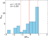 |
Fig. C.1. ΔRFe distribution. Although the fairly large spread, the mean relative difference is close to zero, thus our estimates are not systematically offset with respect to the SDSS control sample. |
Appendix D: Spectral fits of the faint AGNs composite spectra
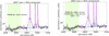 |
Fig. D.1. Spectral modelling of the Hβregion of the low-luminosity composite spectrum assuming only one NLR component (left) and two NLR components (right), one of them accounting for an outflow component. The colour-coding is the same as in Fig.2. The improvement in the best fit BIC is significant (ΔBIC=-116). The FWHM of the broad [O III] (azure) is significantly smaller than that of the broad Hβsupposedly tracing the BLR (red). |
In this section we show the spectral fits of the low-luminosity composite spectra shown in Fig. 3. The colour-coding is the same as in Fig. 2. In the left panel we show the fit without the broad component for the [O III] doublet (light blue), while in the right figure it is included. There, we also report the values of the broad Hβ(red) and [O III] FWHM values, which are significantly different. This difference discourages the outflow interpretation of the broad Hβcomponent.
Appendix E: Fits atlas
Here, we present the complete atlas of the spectral fits described in 3.1, together with the rest-frame spectra. Lines produced in the BLR are highlighted in red, those arising from the NLR in light blue, the Fe II is marked in green, while the power-law continuum is shown in blue. The various component are labelled as described in the top left plot. We also highlight in green the region where we evaluated the Fe II EW. Regions where the data are affected by extremely low S/N or artifacts are covered by a dark grey band. The last figure of the fourth panel includes the spectral fit of the SDSS composite spectrum shown in Fig.3 to highlight the differences with respect to the JWST one.
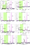 |
Fig. E.1. Fits atlas. |
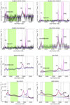 |
Fig. E.1. Continued. |
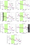 |
Fig. E.1. Continued. |
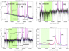 |
Fig. E.1. Continued. |
Appendix F: Photoionisation models with realistic SEDs
In this appendix we investigate the effect of using different SEDs on the predicted RFe. Differently from the default parametric AGNs SEDs from CLOUDY used in the main text, here we take advantage of SEDs constructed from multiwavelength observations of AGNs by Jin et al. (2012, 2017). Figure F1 shows a comparison between the CLOUDY SEDs and SEDs of Jin et al. (2012, 2017) with different Eddington ratios, which are also used by Ferland et al. (2020) to investigate BLR emission. The AGNs SEDs with sub-Eddington ratios all show significant non-thermal X-ray emission comparable or higher than the default CLOUDY SED with αox = −1.4 we adopt. The peak of the big blue bump is shifted to higher energies with increasing Eddington ratios, corresponding to hotter accretion discs. At the highest Eddington ratio of λEdd = 4.6, the SED from Jin et al. (2017) shows a very steep X-ray slope with little non-thermal X-ray component at 1 - 10 keV. In this regime the geometry of the accretion disc might have changed, which leads to trapping of high-energy photons. The thermal disc emission becomes the dominant component in the UV-X-ray regime, similar to the single-disc model we adopt by setting αox = −5 in CLOUDY.
In Figure F2 we show RFe predicted by CLOUDY photoionisation models generated using SEDs of Jin et al. (2012, 2017). We have set NH = 1024 cm−2, nH = 1011 cm−3, and kept all other parameters fixed to the same values as those in Table 3. A similar behavior in these models as those generated using CLOUDY SEDs in Figure 8 can be observed. To explain the low RFe of JWST-selected AGNs, metallicities lower than Z/Z⊙ < 0.2 are needed, consistent with our conclusions drawn from models based on CLOUDY SEDs. Of course, this comparison does not exclude the effects of other model parameters that are fixed, such as nH. Variations of other model parameters are discussed in Section 5.4 and Appendix G.
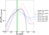 |
Fig. F.1. Comparison between different input SEDs for CLOUDY photoionisation models. All models are normalised to their fluxes at 1 Ryd. The solid and dashed curves correspond to SEDs constructed from the parametric function in CLOUDY. The dash-dotted and dotted curves are SEDs constructed from observations of AGNs by Jin et al. (2012, 2017). The left edge and the right edge of the shaded region correspond to the ionisation potential of Fe0 and Fe+, respectively. |
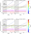 |
Fig. F.2. Comparison between CLOUDY-predicted RFe generated with SEDs from Jin et al. (2012, 2017) and RFe measured from observations. Models are colour-coded according to their ionisation parameters. The range of metallicities derived from narrow lines observed in JWST-selected type 1 AGNs is indicated by the vertical grey shaded region. With these SEDs constrained by observations, low metallicities are still needed to explain the low RFe in our sample of JWST-selected AGNs. |
Appendix G: Photoionisation models with varying densities
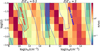 |
Fig. G.1. Photoionisation models predicted RFe as a function of the ionisation parameter and hydrogen density. Left: Models with a subsolar metallicity of Z/Z⊙ = 0.2 plausible for BLRs of low-luminosity AGNs observed by JWST. Right: Models with a super solar metallicity of Z/Z⊙ = 2 plausible for BLRs of local AGNs as well as high-luminosity quasars observed in SDSS. In both panels, the mean RFe of JWST identified AGNs is indicated by the solid red contour, and the mean RFe of SDSS AGNs is indicated by the dashed blue contour. |
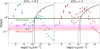 |
Fig. G.2. RFe as a function of the product of U ⋅ nH predicted by our photoionisation models as well as the relation from Panda (2022). The cyan and red circles are the same models shown in Figure G1. The solid black curve and the dotted black curve are relations from Panda (2022) assuming solar metallicity, Gaussian broad Hβ profile, and black hole masses of 107 M⊙ and 108 M⊙ typical for JWST-selected BL AGNs. |
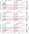 |
Fig. G.3. Comparison between CLOUDY-predicted RFe generated with different densities and RFe measured from observations. Models are colour-coded according to their ionisation parameters. The range of metallicities derived from narrow lines observed in JWST-selected type 1 AGNs is indicated by the vertical grey shaded region. Both low-density (nH < 1010 cm−3) and high-density (nH > 1012 cm−3) models struggle to reproduce RFe of JWST-selected AGNs, especially the X-ray weak ones, which constitute the majority of the sample. |
In this appendix we present additional photoionisation models with a range of hydrogen densities from 108 cm−3 to 1016 cm−3. In Figure G1 we show two sets of AGNs BLR models with subsolar and super-solar metallcities. Apart from the hydrogen density and the metallicity, all other parameters are set to be the same as described in Table 3. It is clear that for both sets of models, local maxima of RFe are found for certain combinations of U and nH, a phenomenon already noted by previous modelling works (e.g. Baldwin et al. 2004; Ferland et al. 2009).
As a comparison, we also show the contours corresponding to the means of JWST identified and SDSS type 1 AGNs with similar FWHMHβ,br and LHβ,br, respectively. Compared to the subsolar metallicity models (Z = 0.2 Z⊙), the JWST AGNs mean is found for 1010 cm−3 < nH < 1012 cm−3. In contrast, the super-solar metallicity models (Z = 2 Z⊙) only match the JWST AGNs mean when nH ≳ 1016 cm−3. The SDSS mean can be found at 1010 cm−3 < nH < 1012 cm−3, nH ≲ 109 cm−3, or nH ≳ 1015 cm−3 compared to the super-solar metallicity models depending on the value of U, or a broader density range compared to the subsolar metallicity models.
More recently, Panda (2022) discussed the relation between RFe and the ionising flux in the BLR (i.e. U ⋅ nH) using observations of reverberation-mapped AGNs as well as theoretical photoionisation models. Figure G2 shows a comparison between our models and the relation of Panda (2022) (their Equation 20) in the RFe versus U ⋅ nH space. The relation of Panda (2022) describes the higher end of U ⋅ nH, where the lower peak at U ⋅ nH < 108 is excluded, as Panda (2022) argues that this is the regime where dust is not destroyed. Our models capture the increasing RFe with U ⋅ nH, although there is a drop at high U ⋅ nH, which is also visible in Panda (2022)’s model in, for example, their Figure 6. As metallicity increases, model points are shifted to higher RFe as expected (Panda 2022’s relation assumes a solar metallicity). As a result, the SDSS RFe is either described by a more intense ionising radiation at low metallicities compared to the JWST RFe, or it is caused by a higher metallicity of SDSS AGNs, or it is caused by an extreme ionising radiation of JWST AGNs. Still, describing SDSS analogs at low metallicity or JWST AGNs at high metallicities, while excluding low ionising flux regimes as Panda (2022), one would need very high U ⋅ nH, potentially reaching 1012 or higher, not seen in, for example, any reverberation-mapped AGNs studied by Panda (2022).
Finally, in Figure G3, we show a more detailed comparison between individual models with fixed densities up to nH = 1013 cm−3, where the highest density is the same as considered by Panda et al. (2020) and Panda (2022). As can be seen in this figure, models with nH < 1010 cm−3 have difficulties reproducing the observed RFe of JWST-selected type 1 AGNs. For 1010 cm−3 ≤ nH ≤ 1012 cm−3, RFe of JWST-selected type 1 AGNs, especially those of the X-ray weak ones, can be reproduced by low-metallicity models given the range of U we consider and the NH we set. At nH = 1013 cm−3, RFe becomes too large compared to the observed RFe of JWST sources over the whole parameter space of Z/Z⊙ and U we consider. Again, this shows that in addition to the metallicity difference, the higher RFe in SDSS analogs compared to JWST sources can be produced by a systematic change in nH between the two samples, as already shown in Figure G1.
While Figures G1, G2, and G3 illustrate the complex degeneracies between model parameters, as we have discussed in Sect. 5.4, based on the current observational evidence it might be more natural to assume redshift evolution in the metallicity rather than other model parameters for BLRs. A scenario invoking the redshift evolution in the gas density, for example, would require ultra-dense environments for JWST-identified AGNs assuming they are similarly metal enriched as SDSS AGNs. At extremely high densities, the strength of permitted UV lines from the BLR would change significantly (Temple et al. 2021), which could be tested observationally using medium-to-high resolution UV follow-ups of less obscured early AGNs with JWST. However, this is beyond the scope of the current work and we leave it for future investigations.
All Tables
All Figures
|
Fig. 1. log(FWHMHβ, br)−log(LHβ, br) parameter space for our BL AGNs (T1AGNs) and the reference samples (SDSS dr17, Shen 2016 S16, Matthews et al. 2021 M21, and Deconto-Machado et al. 2023 DM23), where the SDSS dr17 AGNs are shown with contours. We also include the three BL AGNs in metal-poor dwarf galaxies (DG-T1AGNs). The dashed line marks the threshold luminosity dividing the high- and the low-luminosity sub-samples. The actual log(LHβ, br) of SBS_0335-052E (black thick edge) is 38.3, but it was shifted to 40.0 for the sake of a tighter image layout. The azure and black rectangles mark the regions adopted to define the control samples (Sect. 4). |
| In the text | |
|
Fig. 2. Examples of the spectral fits of a low-luminosity (left) and a high-luminosity (right) AGN of the sample. The different components are colour-coded as stated in the legend. The uncertainty on the data is shown as a shaded area. The Fe II pseudo-continuum is highlighted in green. The vertical grey dashed lines mark the most prominent emission lines. All the spectral fits are shown in E.1. |
| In the text | |
|
Fig. 3. Continuum-subtracted spectral composites of the low-luminosity (left) and high-luminosity (right) subsamples. The Hβand [O III] narrow components have been cut for visualisation purposes. In the right panel we also show the composite quasar spectra for the high-luminosity subsamples. In the case of the Deconto-Machado et al. (2023) sample we built different composite spectra for the Pop A and Pop B sub-samples, which occupy different regions of the EV1 plane. The iron bump between 4434–4684 Å (green shaded area) is evidently weaker in the JWST low-luminosity sample than in the local AGNs. Although the strength of the Fe II bump seemingly varies among the sub-samples, the RFe of the quasars at the epoch of reionisation analysed here is not significantly different from those estimated at lower z as also shown in Table 2. |
| In the text | |
|
Fig. 4. RFe-log(FWHMHβ, br)−log(LHβ, br) plane. Specifically, he have log(FWHMHβ, br) versus log(LHβ, br) colour-coded by RFe. Objects marked with a circle represent RFe upper limits as defined in the text. The background 2D histogram is obtained by binning the control sample (with a minimum of 30 objects per bin); individual objects from JWST are colour-coded with the same scale in RFe. Due to the large number of upper limits in the low-luminosity region, we also include the values derived from the composite spectra as symbols with thicker black edges. The coloured rectangles mark the regions where the control samples were drawn. The black solid arrow marks the direction of the PCA, as described in Sect. 5.2. SBS_0335-052E (black thick edge pentagon) has been shifted for a tighter image layout. |
| In the text | |
|
Fig. 5. Orthogonal sections of the log(FWHMHβ,br)−log(LHβ,br)−RFe parameter space. Specifically we have (left) RFe versus log(LHβ, br) in (colour-coded) bins of FWHMHβ,br, and (right) RFe versus FWHMHβ,br in (colour-coded) bins of log(LHβ, br). The thick-edged diamond and star represent the values derived from the composite spectra. The colour-coded lines represent the third quantity evaluated on the binned sources of the control samples. SBS_0335-052E (black thick edge pentagon) has been shifted for a tighter image layout. It is clear that, while the high-luminosity objects of the sample reside – albeit with some scatter – in the expected locus of the parameter space according to the control sample, the low-luminosity objects exhibit far lower RFe. Interestingly, two low-luminosity objects (JADES-029777 and XID2028) detach from the bulk of the faint sample, being close to the RFe expected. As we discuss further in Sect. 5.5, these are the two only faint AGNs that are X-ray detected. |
| In the text | |
|
Fig. 6. log(EW[O III])–log(RFe) section of the 4DE1. The pink dots mark the SDSS objects selected as a control sample. The blue line highlights the best linear fit to the SDSS data. The thick-edged diamonds represent the average values for the faint JWST AGNs as described in the text. |
| In the text | |
|
Fig. 7. Distributions of the SDSS analogues and our JWST faint AGNs sample in the log([O III]/H[[INLINE259]]])-log(RFe) plane with the O32 ratio colour-coded (except for the faint AGNs where the [O II] was not measured). White contours show the distribution of SDSS AGNs. The diamond with thicker black edges represents the value derived from the low-luminosity composite spectrum. Alongside the main anti-correlation, a secondary branch of SDSS objects detaches (the dashed lines guide the eye along the two branches), which still shares O32 values similar to those of the main trend. Notably, the JWST low-luminosity sources follow this steeper anti-correlation trail, likely driven by low metallicity as explained in the text. |
| In the text | |
|
Fig. 8. Comparisons between RFe predicted by photoionisation models with different input parameters and RFe measured in our sample. In each panel, the green line indicates the mean RFe found in the SDSS sample that matches the JWST sample in terms of Hβluminosities and FWHM; the magenta shaded region corresponds to the value found in the JWST sample; the red shaded region corresponds to the value found in the JWST sample excluding sources with X-ray detections, which also happen to be the strongest Fe II emitters among the faint AGNs. The grey shaded region indicates the plausible range of metallicities in the NLRs of the JWST sources based on the Te method for a subset of the JWST sample. Photoionsation model predictions are plotted as a function of the metallicity, Z/Z⊙, and are colour-coded by the ionisation parameter. Left: solid lines and dashed lines correspond to models with and without a hard X-ray component representing the hot corona contribution to the SED, respectively, Right: solid lines and dashed lines correspond to models having NH = 1024 cm−2 and NH = 1025 cm−2, respectively. |
| In the text | |
|
Fig. C.1. ΔRFe distribution. Although the fairly large spread, the mean relative difference is close to zero, thus our estimates are not systematically offset with respect to the SDSS control sample. |
| In the text | |
|
Fig. D.1. Spectral modelling of the Hβregion of the low-luminosity composite spectrum assuming only one NLR component (left) and two NLR components (right), one of them accounting for an outflow component. The colour-coding is the same as in Fig.2. The improvement in the best fit BIC is significant (ΔBIC=-116). The FWHM of the broad [O III] (azure) is significantly smaller than that of the broad Hβsupposedly tracing the BLR (red). |
| In the text | |
|
Fig. E.1. Fits atlas. |
| In the text | |
|
Fig. E.1. Continued. |
| In the text | |
|
Fig. E.1. Continued. |
| In the text | |
|
Fig. E.1. Continued. |
| In the text | |
|
Fig. F.1. Comparison between different input SEDs for CLOUDY photoionisation models. All models are normalised to their fluxes at 1 Ryd. The solid and dashed curves correspond to SEDs constructed from the parametric function in CLOUDY. The dash-dotted and dotted curves are SEDs constructed from observations of AGNs by Jin et al. (2012, 2017). The left edge and the right edge of the shaded region correspond to the ionisation potential of Fe0 and Fe+, respectively. |
| In the text | |
|
Fig. F.2. Comparison between CLOUDY-predicted RFe generated with SEDs from Jin et al. (2012, 2017) and RFe measured from observations. Models are colour-coded according to their ionisation parameters. The range of metallicities derived from narrow lines observed in JWST-selected type 1 AGNs is indicated by the vertical grey shaded region. With these SEDs constrained by observations, low metallicities are still needed to explain the low RFe in our sample of JWST-selected AGNs. |
| In the text | |
|
Fig. G.1. Photoionisation models predicted RFe as a function of the ionisation parameter and hydrogen density. Left: Models with a subsolar metallicity of Z/Z⊙ = 0.2 plausible for BLRs of low-luminosity AGNs observed by JWST. Right: Models with a super solar metallicity of Z/Z⊙ = 2 plausible for BLRs of local AGNs as well as high-luminosity quasars observed in SDSS. In both panels, the mean RFe of JWST identified AGNs is indicated by the solid red contour, and the mean RFe of SDSS AGNs is indicated by the dashed blue contour. |
| In the text | |
|
Fig. G.2. RFe as a function of the product of U ⋅ nH predicted by our photoionisation models as well as the relation from Panda (2022). The cyan and red circles are the same models shown in Figure G1. The solid black curve and the dotted black curve are relations from Panda (2022) assuming solar metallicity, Gaussian broad Hβ profile, and black hole masses of 107 M⊙ and 108 M⊙ typical for JWST-selected BL AGNs. |
| In the text | |
|
Fig. G.3. Comparison between CLOUDY-predicted RFe generated with different densities and RFe measured from observations. Models are colour-coded according to their ionisation parameters. The range of metallicities derived from narrow lines observed in JWST-selected type 1 AGNs is indicated by the vertical grey shaded region. Both low-density (nH < 1010 cm−3) and high-density (nH > 1012 cm−3) models struggle to reproduce RFe of JWST-selected AGNs, especially the X-ray weak ones, which constitute the majority of the sample. |
| In the text | |
Current usage metrics show cumulative count of Article Views (full-text article views including HTML views, PDF and ePub downloads, according to the available data) and Abstracts Views on Vision4Press platform.
Data correspond to usage on the plateform after 2015. The current usage metrics is available 48-96 hours after online publication and is updated daily on week days.
Initial download of the metrics may take a while.