© The Authors 2025

1. Introduction

Weak gravitational lensing is a powerful probe for studying the distribution of mass in the Universe and constraining cosmological models. Light emitted by distant galaxies is warped by the gravitational field because of over- and under-densities along the line of sight. This effect is typically of the order of a few percent, but it can be observed as coherent shape distortions of source galaxies called ‘cosmic shear’ (for reviews see, e.g. Bartelmann & Schneider 2001; Kilbinger 2015; Mandelbaum 2018). In the past decade, Stage-III photometric surveys such as the Dark Energy Survey (DES; DES Collaboration 2022), the Kilo-Degree Survey (KiDS; Asgari et al. 2021), the Hyper Suprime-Cam survey (HSC; Dalal et al. 2023; Li et al. 2023a) have provided constraints on cosmological parameters from cosmic shear. The Ultraviolet Near-Infrared Optical Northern Survey (UNIONS; Guinot et al. 2022) cosmological analysis is currently in progress and will perform comparable analyses. Forthcoming Stage-IV surveys, such as Euclid (Laureijs et al. 2011; Mellier et al. 2025), the Vera Rubin Observatory Legacy Survey of Space and Time (LSST; Ivezić et al. 2019), and the Nancy Grace Roman Space Telescope (Akeson et al. 2019), will measure cosmic shear with reduced statistical uncertainties thanks to large area coverage and great depth, resulting in a high number density of observed galaxies. Obtaining reliable cosmological results from cosmic shear therefore imposes stringent requirements on controlling and modelling systematic biases and uncertainties that affect cosmic shear measurements.

In practice, to obtain the correct cosmological signal with cosmic shear, one must precisely measure the shapes of galaxies observed in the field of view. However, optical systems can distort the true images of galaxies according to its point spread function (PSF; Mandelbaum 2018). The PSF describes the image response to the light of a point source after passing through atmospheric turbulence and the telescope optics. The observed images correspond to the convolution of the PSF with the images of all observed objects. The PSF can thus modify the shape of galaxies in a systematic way and induce biases and uncertainties in the measurement of galaxy shapes. This effect can be modelled via multiplicative and additive biases that depend on the size and anisotropies of the PSF (Kaiser et al. 1995; Heymans et al. 2006). An error in the size of the PSF results in a multiplicative bias due to an incorrect estimation of how the PSF has rounded the object. Likewise, an error in the PSF shape can give rise to both multiplicative and additive biases. The former can be induced by a coherent alignment or misalignment of the PSF with galaxy shapes (even with a perfect PSF model), and the latter occurs due to modelling errors. The effect of the shape and size mismodelling can be tested statistically using the so-called ρ statistics (Paulin-Henriksson et al. 2008; Jarvis et al. 2016) and the τ statistics (Gatti et al. 2021).

The ρ statistics are the correlations between the PSF ellipticity and its shape and size residuals, whereas the τ statistics cross-correlate those PSF fields with galaxy shapes. The τ statistics provide a null test to identify additive or multiplicative biases but can also be used to estimate the level of systematic uncertainty that propagate to the two-point correlation function, allowing one to forward model the systematic error on the two-point correlation function for cosmological inference.

This estimation of the systematic level requires solving a linear problem that expresses the τ statistics as functions of the ρ statistics and parameters of interest. Estimating those parameters therefore requires a reliable estimate of the covariance matrix of the τ statistics. Previous work used either simulations (Zhang et al. 2023) or jackknife resampling (Gatti et al. 2021) to perform this estimation. The use of simulations, on the one hand, does not easily allow one to capture the whole covariance, as only galaxies (and not stars) are simulated to estimate the covariance. On the other hand, jackknife resampling is based on the hypothesis that the measurement of the τ statistics is sampled from the correct distribution. It also requires build patches of the sky which can be cumbersome in the presence of masks. Finally, the covariance obtained with jackknife resampling tends to be noisier than the one obtained from simulations. It will be useful for future surveys to be able to perform fast PSF diagnostics, i.e. a quick estimation of the τ covariance matrix, to compare galaxy catalogues obtained under different modelling choices.

In this paper, we introduce a semi-analytical method to compute the covariance matrix of the τ statistics and therefore estimate the level of systematic error on the two-point correlation function. We also show how least-square minimisation provides a fast estimation of systematics parameters and their uncertainties. In addition, we discuss how one can break degeneracies in the parameters defining the PSF error model. This paper is organised as follows. In Sect. 2 we review the ρ and τ statistics and introduce our semi-analytical estimate of the covariance matrix for the τ statistics. We also present our sampling methods of the parameters. In Sect. 3, we introduce the catalogues on which we tested this method and the simulations we used to estimate the covariance matrix. We demonstrate in Sect. 4 that our semi-analytical covariance is in agreement with state-of-the-art jackknife resampling and simulation-based estimates. We discuss the performance and features of our PSF diagnostics estimation in Sect. 5. In addition, we present a reformulation of PSF systematics that reduces degeneracies in the parameters of the model. The paper concludes in Sect. 6.

2. Method

In this section, we first introduce our general notation for spin-2 fields, their correlation functions, and estimators (see Sect. 2.1). We then introduce shear and PSF (residual) fields and their relation to observable quantities before reviewing the ρ and τ statistics (see Sects. 2.1–2.3). We discuss the inference problem of the PSF contamination parameters and introduce our least-squares approach to solve it (see Sect. 2.4). Lastly, we describe how we developed the semi-analytical covariance for the τ statistics (see Sect. 2.5).

2.1. Second-order correlations and estimators for spin-2 fields

For two statistically isotropic and homogeneous random fields, a and b, their joint two-point correlation ⟨a(θ)b(θ+ϑ)⟩ between two angular positions, θ and θ + ϑ, only depends on the modulus of the vector between the two positions, ϑ. Under the ergodic principle, the ensemble average can be replaced with a spatial average, and we write

$$\begin{array}{c}\hfill \langle ab\rangle (\vartheta )={\langle a(\mathit{\theta })b(\mathit{\theta }+\mathit{\vartheta })\rangle }_{\mathit{\theta }}.\end{array}$$(1)

Shear and ellipticity are spin-2 fields, and they can be written in complex notation as a = a₁ + ia₂ = |a|exp(2iφ). Here, the real (resp. imaginary) part of the field, a₁ (resp. a₂), quantifies the amplitude of the ellipticity of the object oriented at a 0 (resp. 45) degree angle with respect to the x-axis in a local Cartesian coordinate system. The phase, φ, denotes the orientation of the ellipse.

For a pair of galaxies with connecting vector ϑ and polar angle ϕ, the shear of both galaxies is conveniently rotated into the coordinate system, where ϑ is the first coordinate direction. This defines the tangential and cross components of the shear, a_t and a_×, respectively, as

$$\begin{array}{c}\hfill a_{\mathrm{t}}=\mathfrak{R}\left(a{\mathrm{e}}^{-2\mathrm{i}\varphi }\right);a_{\times }=\mathfrak{I}\left(a{\mathrm{e}}^{-2\mathrm{i}\varphi }\right).\end{array}$$(2)

The two standard parity-invariant correlation functions (Schneider et al. 2002) for the spin-2 fields, a and b, are defined as

$$\begin{array}{cc}\hfill {\xi }_{+}^{\mathit{ab}}(\vartheta )& =\langle a_{\mathrm{t}}{b}_{\mathrm{t}}\rangle (\vartheta )+\langle a_{\times }{b}_{\times }\rangle (\vartheta )\hfill \\ \hfill & =\langle a_1{b}_1\rangle (\vartheta )+\langle a_2{b}_2\rangle (\vartheta )\hfill \\ \hfill & =\mathfrak{R}\left[⟨a{b}^{\ast }⟩(\vartheta )\right];\hfill \\ \hfill {\xi }_{-}^{\mathit{ab}}(\vartheta )& =\langle a_{\mathrm{t}}{b}_{\mathrm{t}}\rangle (\vartheta )-\langle a_{\times }{b}_{\times }\rangle (\vartheta )\hfill \\ \hfill & =\langle [\left(a_1{b}_1\right)(\vartheta )-\left(a_2{b}_2\right)(\vartheta )]cos4\varphi \rangle \hfill \\ \hfill & +\langle [\left(a_1{b}_2\right)(\vartheta )+\left(a_2{b}_1\right)(\vartheta )]sin4\varphi \rangle \hfill \\ \hfill & =\mathfrak{R}\langle \left(ab\right)(\vartheta )e^{-4\mathrm{i}\varphi }\rangle .\hfill \end{array}$$(3)

Parity-violating correlation functions are reproduced in Appendix A. Following Schneider et al. (2002), estimators of the correlation functions (3) are

$$\begin{array}{cc}\hfill {\widehat{\xi }}_{+}^{\mathit{ab}}(\vartheta )=& \frac{1}{N_{\mathrm{p}}^{\mathit{ab}}(\vartheta )}{\displaystyle \sum _{\mathit{ij}}}{w}_i^a{w}_j^b{\mathrm{\Delta }}_{\vartheta }({\vartheta }_{\mathit{ij}})(a_{i1}{b}_{j1}+a_{i2}{b}_{j2})\hfill \\ \hfill =& \frac{1}{N_{\mathrm{p}}^{\mathit{ab}}(\vartheta )}{\displaystyle \sum _{\mathit{ij}}}{w}_i^a{w}_j^b{\mathrm{\Delta }}_{\vartheta }({\vartheta }_{\mathit{ij}}){\displaystyle \sum _{\alpha =1}^2}{a}_{i\alpha }{b}_{j\alpha };\hfill \\ \hfill {\widehat{\xi }}_{-}^{\mathit{ab}}(\vartheta )=& \frac{1}{N_{\mathrm{p}}^{\mathit{ab}}(\vartheta )}{\displaystyle \sum _{\mathit{ij}}}{w}_i^a{w}_j^b{\mathrm{\Delta }}_{\vartheta }({\vartheta }_{\mathit{ij}})\hfill \\ \hfill & \times [(a_{i1}{b}_{j1}-a_{i2}{b}_{j2})cos4{\varphi }_{\mathit{ij}}+(a_{i1}{b}_{j2}+a_{i2}{b}_{j1})sin4{\varphi }_{\mathit{ij}}].\hfill \end{array}$$(4)

Here, $N_{\mathrm{p}}^{\mathit{ab}}(\vartheta )$ is the number of pairs of objects sampling the fields a and b in the angular bin around ϑ given as

$$\begin{array}{c}\hfill N_{\mathrm{p}}^{\mathit{ab}}={\displaystyle \sum _{\mathit{ij}}}{w}_i^a{w}_j^b{\mathrm{\Delta }}_{\vartheta }({\vartheta }_{\mathit{ij}}).\end{array}$$(5)

The sums are carried out over all objects, i, sampling field a, and all objects, j, sampling field b, whose pair-wise distance, ϑ_ij, is within the angular bin around ϑ. The bin is given by Δ_ϑ(ϑ_ij) = 1_{[ϑ − Δϑ/2; ϑ + Δϑ/2]}(ϑ_ij), where the indicator function 1_S(x) is 1 if x ∈ S and 0 otherwise.

The ellipticity or shear of each object, a_i (resp. b_j), has an associated weight, w_i^a (resp. w_j^b). Those weights account for variable signal-to-noise ratios for the different objects that introduce uncertainty in the shape measurement (see, e.g. Gatti et al. 2021).

In the following, we reproduce useful relations adapted from Schneider et al. (2002) for the correlation of two spin-2 fields, a and b. Their derivation with the inclusion of parity-violating correlations is detailed in Appendix A.

$$\begin{array}{cc}\hfill ⟨a_{i1}{b}_{j1}⟩& =\frac{1}{2}[{\xi }_{+}^{\mathit{ab}}({\vartheta }_{\mathit{ij}})+{\xi }_{-}^{\mathit{ab}}({\vartheta }_{\mathit{ij}})cos4{\varphi }_{\mathit{ij}}-{\xi }_{\times }^{\mathit{ab}}({\vartheta }_{\mathit{ij}})sin4{\varphi }_{\mathit{ij}}];\hfill \\ \hfill ⟨a_{i2}{b}_{j2}⟩& =\frac{1}{2}[{\xi }_{+}^{\mathit{ab}}({\vartheta }_{\mathit{ij}})-{\xi }_{-}^{\mathit{ab}}({\vartheta }_{\mathit{ij}})cos4{\varphi }_{\mathit{ij}}+{\xi }_{\times }^{\mathit{ab}}({\vartheta }_{\mathit{ij}})sin4{\varphi }_{\mathit{ij}}];\hfill \\ \hfill ⟨a_{i1}{b}_{j2}⟩& =\frac{1}{2}[{\xi }_{-}^{\mathit{ab}}({\vartheta }_{\mathit{ij}})sin4{\varphi }_{\mathit{ij}}+{\xi }_{\times }^{\mathit{ab}}({\vartheta }_{\mathit{ij}})cos4{\varphi }_{\mathit{ij}}-{\xi }_{\ast }^{\mathit{ab}}({\vartheta }_{\mathit{ij}})];\hfill \\ \hfill ⟨a_{i2}{b}_{j1}⟩& =\frac{1}{2}[{\xi }_{-}^{\mathit{ab}}({\vartheta }_{\mathit{ij}})sin4{\varphi }_{\mathit{ij}}+{\xi }_{\times }^{\mathit{ab}}({\vartheta }_{\mathit{ij}})cos4{\varphi }_{\mathit{ij}}+{\xi }_{\ast }^{\mathit{ab}}({\vartheta }_{\mathit{ij}})].\hfill \end{array}$$(6)

Under the assumption that ξ_× (see Eq. (A.1)) vanishes and with a = b, the first two equations reduce to Eq. (22) in Schneider et al. (2002). Additionally, with ξ_* = 0, the sum of our third and fourth equations equals twice the mixed expression from their Eq. (22). In what follows, we set ξ_× = 0 and ξ_* = 0, corresponding to parity conservation of the fields a and b.

2.2. Shear and PSF (residual) ellipticity

In general, shear (γ) is estimated by the observed shape of background galaxies, quantified by an ellipticity measurement, e^obs. This is a noisy estimate, with the intrinsic (source) galaxy ellipticity, e^s, serving as a stochastic element. We assumed an additive systematic contribution, e^sys, stemming from the PSF, and thus

$$\begin{array}{c}\hfill e\equiv e^{\mathrm{obs}}=e^{\mathrm{s}}+e^{\mathrm{PSF},\mathrm{sys}}+\gamma .\end{array}$$(7)

We assumed that the observed ellipticity has been calibrated for multiplicative biases. While we expect ⟨e^s⟩ = 0 in the absence of intrinsic alignment, a non-zero ⟨e^PSF, sys⟩ would be a smoking gun for a systematic PSF contribution to the measured shapes of galaxies. A commonly used linear model for the PSF contribution is

$$\begin{array}{c}\hfill e^{\mathrm{PSF},\mathrm{sys}}=\alpha e^{\mathrm{p}}+\beta \delta e^{\mathrm{p}}+\eta \delta T^{\mathrm{p}},\end{array}$$(8)

where e^p is the ellipticity of the PSF, δe^p = e^* − e^p denotes the ellipticity residual (measured at star positions), and δT^p = e^*(T^* − T^p)/T^* is the size residual, also defined at star positions. The size term is multiplied by the star ellipticity, e^*, to define a spin-2 field, consistent with Paulin-Henriksson et al. (2008). Other models can and have been used as well (e.g. Giblin et al. 2021; Zhang et al. 2023, 2024). The first term in Eq. (8) corresponds to a spurious dependence of the measured shape on the PSF, the so-called PSF leakage. Such a leakage might be introduced by an imperfect deconvolution of the observed galaxy image by the PSF. The second and third terms in the above equation quantify PSF modelling and interpolation errors.

The PSF and its residuals were estimated from measurements of the ellipticity of stars and the PSF model. The PSF ellipticity and size are exact and deterministic once the PSF model is fixed. The ellipticity and size of stars were measured with a small amount of stochasticity since stars are point sources and are typically selected at a high signal-to-noise ratio. In addition, there is pixel noise, unresolved binaries, cosmic rays, and saturation effects, among other elements. Those effects introduce a stochastic element in measuring star ellipticity. Likewise, the atmosphere for ground-based observations is stochastic, but this stochasticity is part of the PSF at a given observation epoch, sky, and focal plane position – the atmosphere is part of the ‘signal’ and not the noise.

The estimate for the shot noise for galaxies, ∑_i|e_i|²/N, is a very good approximation of ⟨|e^s|²⟩ since ⟨|γ|²⟩ is much smaller and can fairly safely be neglected. In contrast, for the reasons stated above, the star and PSF parameters are dominated by the signal over the noise. The estimation of shot noise is therefore not straightforward. In addition, the size residual is a combination of star ellipticity and size, which might be correlated.

As we describe in detail in Sect. 2.5.1, the inclusion of the estimated shot noise for the star and PSF parameters leads to an incorrect semi-analytical covariance matrix of the galaxy-PSF cross-correlation functions. For this reason, unlike in Eq. (7), where the intrinsic shape of galaxies, e^s, is taken into account, we do not include a stochastic ellipticity, b^s, in the relation between observed and true PSF quantities. Instead, the shot noise of the galaxy-PSF cross-correlation functions were measured from the data and added independently to the semi-analytical covariance matrix. Here, we write the relation between observed and true star and PSF parameters as

$$\begin{array}{c}\hfill b^{\mathrm{obs}}=b\text{for}b\in \{e^{\mathrm{p}},\delta e^{\mathrm{p}},\delta T^{\mathrm{p}}\}.\end{array}$$(9)

2.3. ρ statistics

The ρ statistics are cross-correlation functions of the PSF-related fields appearing in the systematic error contribution to Eq. (8). They are defined as follows (see Rowe 2010; Jarvis et al. 2016; Gatti et al. 2021):

$$\begin{array}{cccc}\hfill {\rho }_0(\vartheta )& =⟨e^{\mathrm{p}}{e}^{\mathrm{p}}⟩(\vartheta );\hfill & \hfill {\rho }_1(\vartheta )& =⟨\delta e^{\mathrm{p}}\delta e^{\mathrm{p}}⟩(\vartheta );\hfill \\ \hfill {\rho }_2(\vartheta )& =⟨e^{\mathrm{p}}\delta e^{\mathrm{p}}⟩(\vartheta );\hfill & \hfill {\rho }_3(\vartheta )& =⟨\delta T^{\mathrm{p}}\delta T^{\mathrm{p}}⟩(\vartheta );\hfill \\ \hfill {\rho }_4(\vartheta )& =⟨\delta e^{\mathrm{p}}\delta T^{\mathrm{p}}⟩(\vartheta );\hfill & \hfill {\rho }_5(\vartheta )& =⟨e^{\mathrm{p}}\delta T^{\mathrm{p}}⟩(\vartheta ).\hfill \end{array}$$(10)

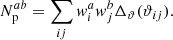
We abused the notation ⟨.⟩ for simplicity. In practice, each ρ statistic has a +, −, , and × component obtained using Eqs. (3) and (A.1) with the corresponding field a and b (e.g. ρ_0, ± = ξ_±^epep). Those statistics quantify the contributions to additive bias of the shear two-point correlation function.

Under the linear model (8), we cannot quantify the systematic error with the ρ statistics alone, as it depends on the value of the parameters α, β, and η. Hence, we needed to compute cross-correlations between galaxies and the PSF fields to estimate those parameters.

2.4. τ statistics

The τ statistics (Hamana et al. 2020; Giblin et al. 2021; Gatti et al. 2021; Zhang et al. 2023) were obtained by cross-correlating the galaxy ellipticities with the different PSF terms appearing in Eq. (8):

$$\begin{array}{c}\hfill {\tau }_0(\vartheta )=⟨e{e}^{\mathrm{p}}⟩(\vartheta );{\tau }_2(\vartheta )=⟨e\delta e^{\mathrm{p}}⟩(\vartheta );{\tau }_5(\vartheta )=⟨e\delta T^{\mathrm{p}}⟩(\vartheta ),\end{array}$$(11)

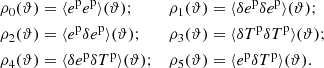
where we use the same abuse of notation as in the above section. The galaxy ellipticities, e, appearing in the definition of the τ statistics have been calibrated (see Sect. 3 for details on the calibration) and mean subtracted to remove a non-zero ⟨γ⟩ due to cosmic variance. Interestingly, those correlators allowed us to fit a model to estimate the value of α, β, and η using the following linear equations for a given scale, ϑ:

$$\begin{array}{cc}\hfill {\tau }_0(\vartheta )& =\alpha {\rho }_0(\vartheta )+\beta {\rho }_2(\vartheta )+\eta {\rho }_5(\vartheta );\hfill \\ \hfill {\tau }_2(\vartheta )& =\alpha {\rho }_2(\vartheta )+\beta {\rho }_1(\vartheta )+\eta {\rho }_4(\vartheta );\hfill \\ \hfill {\tau }_5(\vartheta )& =\alpha {\rho }_5(\vartheta )+\beta {\rho }_4(\vartheta )+\eta {\rho }_3(\vartheta ).\hfill \end{array}$$(12)

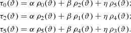
One can choose to invert the system of equations at each scale or to consider scale-independent parameters α, β, and η. For simplicity and because the ρ and τ statistics are noisy, we assume in this work that these parameters are scale independent. The linear equations per scale (12) can be concatenated into a single matrix equation:

$$\begin{array}{c}\hfill \left(\begin{array}{c}{\tau }_{0,1}\hfill \\ {\tau }_{2,1}\hfill \\ {\tau }_{5,1}\hfill \\ ⋮\hfill \\ {\tau }_{0,n}\hfill \\ {\tau }_{2,n}\hfill \\ {\tau }_{5,n}\hfill \end{array}\right)=\left(\begin{array}{ccc}{\rho }_{0,1}\hfill & {\rho }_{2,1}\hfill & {\rho }_{5,1}\hfill \\ {\rho }_{2,1}\hfill & {\rho }_{1,1}\hfill & {\rho }_{4,1}\hfill \\ {\rho }_{5,1}\hfill & {\rho }_{4,1}\hfill & {\rho }_{3,1}\hfill \\ \hfill & \ddots \hfill & \\ {\rho }_{0,n}\hfill & {\rho }_{2,n}\hfill & {\rho }_{5,n}\hfill \\ {\rho }_{2,n}\hfill & {\rho }_{1,n}\hfill & {\rho }_{4,n}\hfill \\ {\rho }_{5,n}\hfill & {\rho }_{4,n}\hfill & {\rho }_{3,n}\hfill \end{array}\right)\left(\begin{array}{c}\alpha \hfill \\ \beta \hfill \\ \eta \hfill \end{array}\right),\end{array}$$(13)

where ρ_i, j denotes the value of the i-th ρ statistics at the j-th angular bin, and similarly τ_i, j is the value of the i-th τ statistics at the j-th angular bin. Equation (13) in short is written as

$$\begin{array}{c}\hfill \mathit{\tau }=\mathbf{R}\mathbf{\Omega }+\mathrm{\Sigma }.\end{array}$$(14)

Here, Ω = (α, β, η)^T and Σ is a noise contribution that can be formally written as a combination of the covariances of ρ and τ statistics: Σ_ρ and Σ_τ.

Solving this linear system allowed us to estimate the level of systematic, which is written as

$$\begin{array}{cc}\hfill {\xi }_{\mathrm{PSF},\mathrm{sys}}(\vartheta )& ={\alpha }^2{\rho }_0(\vartheta )+{\beta }^2{\rho }_1(\vartheta )+{\eta }^2{\rho }_3(\vartheta )\hfill \\ \hfill & +2\alpha \beta {\rho }_2(\vartheta )+2\alpha \eta {\rho }_5(\vartheta )+2\beta \eta {\rho }_4(\vartheta ).\hfill \end{array}$$(15)

This expression represents an additive systematic component to the shear-shear correlation function ξ^γγ. The ρ and τ statistics thus provide a powerful test of the level of systematics as long as the covariance of the τ statistics, Σ_τ, is accurately estimated. The method to estimate that covariance has to date relied on either simulations or jackknife resampling of the data (Zhang et al. 2023; Gatti et al. 2021). The former requires creating many simulations that usually only include galaxy shapes (with the shear following a theoretical power spectrum) and thus does not take into account the contribution from stars and the PSF to the covariance. On the other hand, jackknife resampling is noisy and requires building a sufficiently large number of patches on the sky. In addition, jackknife resampling tends to underestimate the true covariance on large scales (Friedrich et al. 2016). To overcome these limitations and to offer an alternative, we developed a semi-analytical way to compute Σ_τ. The analytical expression of Σ_τ is presented in Sect. 2.5.

To solve the linear system (14), we used two different methods that both require Σ_τ. The first one is a standard Markov chain Monte Carlo (MCMC) sampling a Gaussian likelihood with covariance Σ_τ. The second method solves the following least-square problem:

$$\begin{array}{c}\hfill {\mathbf{\Omega }}^{\ast }={\displaystyle \underset{\mathbf{\Omega }}{\arg \min }}{\Vert \mathit{\tau }-\mathbf{R}\mathbf{\Omega }\Vert }_{{\mathrm{\Sigma }}_{\tau }}^2.\end{array}$$(16)

This problem has an exact solution:

$$\begin{array}{c}\hfill {\mathbf{\Omega }}^{\ast }={({\mathbf{R}}^{\mathrm{T}}{\mathrm{\Sigma }}_{\tau }^{-1}\mathbf{R})}^{-1}{\mathbf{R}}^{\mathrm{T}}\mathit{\tau }.\end{array}$$(17)

To obtain error bars on the parameter estimates from the analytical solution, we sampled ρ and τ statistics from their respective covariances to get a range of solutions of the least-square problem. The covariance of the ρ statistics was computed with jackknife resampling independent of which covariance was used for the τ statistics. We checked that the results were not sensitive to the variation of the ρ statistics covariance from differences in jackknife patch placement. In Sect. 4.3 we compare the results obtained using MCMC chains and least-squares minimisation.

2.5. Semi-analytical covariance

2.5.1. Derivation of the covariance

We developed the covariance for the estimator Eq. (4), ${\widehat{\xi }}_{+}^{\mathit{ab}}$, following Schneider et al. (2002). We reiterate that ${\widehat{\xi }}_{+}^{\mathit{ab}}$ refers to the two-point correlation function estimator of two spin-2 fields, a and b. Those fields can represent the ellipticities of galaxies, the PSF, stars, or the difference between the PSF and stars (PSF residuals) in our context. For the covariance of the three τ statistics (11), the term of interest is the covariance, C, between ${\widehat{\xi }}_{+}^{\mathit{ab}}$ and ${\widehat{\xi }}_{+}^{\mathit{dc}}$ with a = d = e, with b, c being one of the three PSF-related quantities given in Eq. (9). We therefore write

$$\begin{array}{c}\hfill \mathbf{C}({\widehat{\xi }}_{+}^{\mathit{eb}},{\widehat{\xi }}_{+}^{\mathit{ec}};{\vartheta }_1,{\vartheta }_2)=\langle {\widehat{\xi }}_{+}^{\mathit{eb}}({\vartheta }_1){\widehat{\xi }}_{+}^{\mathit{ec}}({\vartheta }_2)\rangle -\langle {\widehat{\xi }}_{+}^{\mathit{eb}}({\vartheta }_1)\rangle \langle {\widehat{\xi }}_{+}^{\mathit{ec}}({\vartheta }_2)\rangle \\ \hfill =& \frac{1}{N_{\mathrm{p}}^{\mathit{eb}}({\vartheta }_1)N_{\mathrm{p}}^{\mathit{ec}}({\vartheta }_2)}{\displaystyle \sum _{\mathit{ijkl}}}{w}_i^e{w}_j^b{w}_k^e{w}_l^c\langle {\displaystyle \sum _{\alpha =1}^2}{e}_{i\alpha }{b}_{j\alpha }{\displaystyle \sum _{\beta =1}^2}{e}_{k\beta }{c}_{l\beta }\rangle \hfill \\ \hfill & -{\xi }_{+}^{\mathit{eb}}({\vartheta }_1){\xi }_{+}^{\mathit{ec}}({\vartheta }_2)\hfill \\ \hfill =& \frac{1}{N_{\mathrm{p}}^{\mathit{eb}}({\vartheta }_1)N_{\mathrm{p}}^{\mathit{ec}}({\vartheta }_2)}{\displaystyle \sum _{\mathit{ijkl}}}{w}_i^e{w}_j^b{w}_k^e{w}_l^c{\displaystyle \sum _{\alpha ,\beta =1}^2}\langle e_{i\alpha }{b}_{j\alpha }{e}_{k\beta }{c}_{l\beta }\rangle \hfill \\ \hfill & -{\xi }_{+}^{\mathit{eb}}({\vartheta }_1){\xi }_{+}^{\mathit{ec}}({\vartheta }_2).\hfill \end{array}$$(18)

This expression involves correlations between four ellipticities ⟨e_iαb_jαe_kβc_lβ⟩, two of which are galaxy estimates, and the other two are PSF ellipticities or PSF residuals. We inserted Eqs. (7) and (9) to expand the four-point correlator. In this expansion, odd-power terms in e^s, γ, b, and c vanish. The shot noise term is zero as well since b and c are modelled without a stochastic contribution. The mixed term consists of the galaxy shot noise and the PSF signal contributions, which is of the form $\langle e_{i\alpha }^{\mathrm{s}}{e}_{k\beta }^{\mathrm{s}}\rangle \langle b_{j\alpha }{c}_{l\beta }\rangle$. The first factor reduces to σ_e²/2 × δ_αβδ_ik. The second factor, after carrying out the sum over the ellipticity components, yields ξ₊^bc(ϑ_jl). In our context, it corresponds to one of the ρ statistics obtained after correlating the fields b and c.

The cosmic-variance term can be split into the connected four-point term and a sum of products of two-point terms, according to Wick’s theorem. Here, as in Schneider et al. (2002), we assumed the fields to be Gaussian and set the connected term to zero. Tests of this assumption are presented in Appendix B, where we use the concept of ‘transcovariance’ matrices (Sellentin & Heavens 2018) to detectnon-Gaussianities. The four-point term is therefore

$$\begin{array}{cc}\hfill ⟨{\gamma }_{i\alpha }{b}_{j\alpha }{\gamma }_{k\beta }{c}_{l\beta }⟩& =⟨{\gamma }_{i\alpha }{b}_{j\alpha }⟩⟨{\gamma }_{k\beta }{c}_{l\beta }⟩+⟨{\gamma }_{i\alpha }{\gamma }_{k\beta }⟩⟨b_{j\alpha }{c}_{l\beta }⟩\hfill \\ \hfill & +⟨{\gamma }_{i\alpha }{c}_{l\beta }⟩⟨{\gamma }_{k\beta }{b}_{j\alpha }⟩,\hfill \end{array}$$(19)

with α, β ∈ {1, 2}, i ≠ j, and k ≠ l. The first term on the right-hand side of Eq. (19) separates into sums over (i, j, α) and (k, l, β), the result of which is ξ₊^γb(ϑ₁)ξ₊^γc(ϑ₂). This product of the means is subtracted in Eq. (18). Using Eq. (6), the remaining terms led to

$$\begin{array}{c}\hfill {\displaystyle \sum _{\alpha ,\beta =1}^2}[\langle {\gamma }_{i\alpha }{\gamma }_{k\beta }\rangle \langle b_{j\alpha }{c}_{l\beta }\rangle +\langle {\gamma }_{i\alpha }{c}_{l\beta }\rangle \langle {\gamma }_{k\beta }{b}_{j\alpha }\rangle ]\\ \hfill =& \frac{1}{2}[{\xi }_{+}^{\gamma \gamma }(ik){\xi }_{+}^{\mathit{bc}}(jl)+{\xi }_{+}^{\gamma c}(il){\xi }_{+}^{\gamma b}(jk)\hfill \\ \hfill & +{\xi }_{-}^{\gamma \gamma }(ik){\xi }_{-}^{\mathit{bc}}(jl)cos(4({\varphi }_{\mathit{ik}}-{\varphi }_{\mathit{jl}}))\hfill \\ \hfill & +{\xi }_{-}^{\gamma c}(il){\xi }_{-}^{\gamma b}(jk)cos(4({\varphi }_{\mathit{il}}-{\varphi }_{\mathit{jk}}))].\hfill \end{array}$$(20)

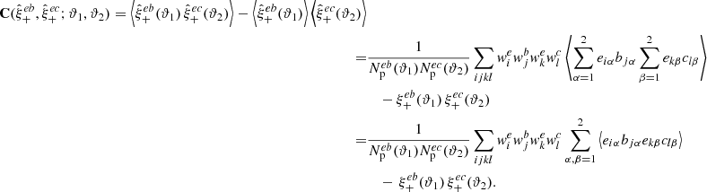
The total covariance is then

$$\begin{array}{c}\hfill \mathbf{C}({\widehat{\xi }}_{+}^{\mathit{eb}},{\widehat{\xi }}_{+}^{\mathit{ec}};{\vartheta }_1,{\vartheta }_2)=\frac{1}{N_{\mathrm{p}}^{\mathrm{eb}}({\vartheta }_1)N_{\mathrm{p}}^{\mathrm{ec}}({\vartheta }_2)}\\ \hfill & \times \{\frac{{\sigma }_e^2}{2}{\displaystyle \sum _{\mathit{ijk}}}{(w_i^e)}^2{w}_j^b{w}_k^c{\mathrm{\Delta }}_{{\vartheta }_1}({\vartheta }_{\mathit{ij}}){\mathrm{\Delta }}_{{\vartheta }_2}({\vartheta }_{\mathit{ik}}){\xi }_{+}^{\mathit{bc}}({\vartheta }_{\mathit{jk}})\hfill \\ \hfill & +\frac{1}{2}{\displaystyle \sum _{\mathit{ijkl}}}{w}_i^e{w}_j^b{w}_k^e{w}_l^c{\mathrm{\Delta }}_{{\vartheta }_1}({\vartheta }_{\mathit{ij}}){\mathrm{\Delta }}_{{\vartheta }_2}({\vartheta }_{\mathit{kl}})\hfill \\ \hfill & \times [({\xi }_{+}^{\gamma \gamma }({\vartheta }_{\mathit{il}}){\xi }_{+}^{\mathit{bc}}({\vartheta }_{\mathit{jk}})+{\xi }_{+}^{\gamma c}({\vartheta }_{\mathit{il}}){\xi }_{+}^{\gamma b}({\vartheta }_{\mathit{jk}}))\hfill \\ \hfill & +({\xi }_{-}^{\gamma \gamma }({\vartheta }_{\mathit{il}}){\xi }_{-}^{\mathit{bc}}({\vartheta }_{\mathit{jk}})+{\xi }_{-}^{\gamma c}({\vartheta }_{\mathit{il}}){\xi }_{-}^{\gamma b}({\vartheta }_{\mathit{jk}}))cos4({\varphi }_{\mathit{il}}-{\varphi }_{\mathit{jk}})]\}.\hfill \end{array}$$(21)

For the cosmic-variance term, we made use of the invariance of each summand under exchange of the indices k and l. As discussed earlier, since we did not add a stochastic element b^s to the PSF fields, the mixed-term is one-fourth of that of Schneider et al. (2002), and the pure shot noise term vanishes. However, if such shot noise is measured in actual data, it cannot be neglected; thus, a caveat of our model is the absence of shot noise. We describe in Sect. 2.5.3 how we take into account the measured shot noise in practice.

2.5.2. Ensemble averages

Given a catalogue containing the different fields involved in the computation of the covariance (21), the latter can be calculated using galaxy positions and their weights. However, the sum over three or even four galaxy positions is not easily tractable given the amount of galaxies in our catalogues. A Monte Carlo approach that draws random simulated galaxy positions distributed uniformly over the survey footprint was developed in Kilbinger & Schneider (2004). Here, we followed Schneider et al. (2002) and replace the sums over galaxy positions by ensemble averages. As in Schneider et al. (2002), we set all weights to unity and considered a survey geometry of solid angle A and galaxy number density n^a for a field a. The number of pairs was approximated as

$$\begin{array}{c}\hfill N_{\mathrm{p}}^{\mathit{ab}}(\vartheta )\approx 2\pi \mathrm{\Delta }\vartheta \vartheta n^a{n}^{b}A.\end{array}$$(22)

The ensemble average for one galaxy corresponds to the area integral over the survey footprint normalised by the survey area. For N galaxies, the ensemble averages for all galaxies are multiplied, resulting in the operator

$$\begin{array}{c}\hfill E={\displaystyle \prod _{i=1}^N}\left(\frac{1}{A}{\displaystyle {\int }_A}{\mathrm{d}}^2{\mathit{\theta }}_i\right).\end{array}$$(23)

For the mixed term, M_e, we took the ensemble average over triplets of object positions. The three catalogues have numbers of objects N^e, N^b, and N^c, respectively. All but three integrals in (23) are trivial and reduce to unity. The sum of triple integrals can be written as N^eN^bN^c permutations of the same expression. With all prefactors, this is then

$$\begin{array}{cc}\hfill E\left[M_e\right]=& \frac{1}{N_{\mathrm{p}}^{\mathit{eb}}({\vartheta }_1)N_{\mathrm{p}}^{\mathit{ec}}({\vartheta }_2)}\frac{{\sigma }_e^2}{2}\frac{N^e{N}^b{N}^c}{A^3}\hfill \\ \hfill & \times {\displaystyle \int {\mathrm{d}}^2}{\theta }_1{\displaystyle \int {\mathrm{d}}^2}{\theta }_2{\displaystyle \int {\mathrm{d}}^2}{\theta }_3{\mathrm{\Delta }}_{{\vartheta }_1}({\theta }_{12}){\mathrm{\Delta }}_{{\vartheta }_2}({\theta }_{13}){\xi }_{+}^{\mathit{bc}}\left({\theta }_{23}\right),\hfill \end{array}$$(24)

where θ_ij = |θ_i − θ_j|. We substituted θ₂′=θ₂ − θ₁ and θ₃′=θ₃ − θ₁; the θ₁-integration could then be carried out trivially to yield the area, A.

Conveniently, we split the area integrals into radial and azimuthal parts. The bin indicator functions restrict θ₂′ (resp. θ₃′) in bins of width Δθ around ϑ₁ (resp. ϑ₂). Assuming that ξ₊^bc does not vary much over the bin width, we could solve the two radial integrals. This led to the intermediate result

$$\begin{array}{cc}\hfill E\left[M_e\right]=& \frac{1}{N_{\mathrm{p}}^{\mathit{eb}}({\vartheta }_1)N_{\mathrm{p}}^{\mathit{ec}}({\vartheta }_2)}\frac{{\sigma }_e^2}{2}\frac{N^e{N}^b{N}^c}{A^2}\mathrm{\Delta }{\vartheta }^2{\vartheta }_1{\vartheta }_2\hfill \\ \hfill & \times {\displaystyle \underset{0}{\overset{2\pi }{\int }}}\mathrm{d}{\phi }_1{\displaystyle \underset{0}{\overset{2\pi }{\int }}}\mathrm{d}{\phi }_2{\xi }_{+}^{\mathit{bc}}\left(\sqrt{{\vartheta }_1+{\vartheta }_2-2{\vartheta }_1{\vartheta }_{2}cos({\phi }_2-{\phi }_1)}\right).\hfill \end{array}$$(25)

One of the angular integrals can be carried out trivially to yield 2π. Expanding the number of pairs, we found, analogously to Schneider et al. (2002),

$$\begin{array}{c}\hfill E\left[M_e\right]=\frac{{\sigma }_e^2}{2\pi A{n}^e}{\displaystyle \underset{0}{\overset{\pi }{\int }}}\mathrm{d}\phi {\xi }_{+}^{\mathit{bc}}\left(\sqrt{{\vartheta }_1^2+{\vartheta }_2^2-2{\vartheta }_1{\vartheta }_{2}cos\phi }\right).\end{array}$$(26)

We note the reduced integration range [0; π] due to the periodicity of the integrand. As expected, this is one-fourth of the corresponding term Eq. (32) in Schneider et al. (2002).

The cosmic-variance term was computed similarly as the mixed term. Under the ensemble average operator Eq. (23), these terms can be written as ≈N^eN^eN^bN^c permutations of a product over four galaxy positions. All three addends of the cosmic-variance term can be written in the form

$$\begin{array}{c}\hfill E\left[V^{\mathrm{term}}\right]=\frac{1}{N_{\mathrm{p}}^{\mathit{eb}}({\vartheta }_1)N_{\mathrm{p}}^{\mathit{ec}}({\vartheta }_2)}\frac{{\left(N^e\right)}^2{N}^b{N}^c}{2A^4}{\displaystyle \int {\mathrm{d}}^2}{\theta }_1{\displaystyle \int {\mathrm{d}}^2}{\theta }_2{\mathrm{\Delta }}_{{\vartheta }_1}({\theta }_{12})\\ \hfill & \times {\displaystyle \int {\mathrm{d}}^2}{\theta }_3{\displaystyle \int {\mathrm{d}}^2}{\theta }_4{\mathrm{\Delta }}_{{\vartheta }_2}({\theta }_{34})F_1({\mathit{\theta }}_{23})F_2({\mathit{\theta }}_{14}).\hfill \end{array}$$(27)

The first two terms depend on the scalars θ₂₃ and θ₁₄. For the third term, we can expand the cosine function into products of cosines and sines, and thus the above separation into F₁ and F₂ is valid.

We performed the variable substitutions ϕ₁ = θ₂ − θ₁ and ϕ₂ = θ₄ − θ₃. Since θ₂₃ = θ₃ − θ₁ − ϕ₁ and θ₄ − θ₁ = θ₃ − θ₁ + ϕ₂, the arguments of F₁ and F₂ only depend on ϕ ≡ θ₁ − θ₃. Therefore, the θ₃-integration can be carried out trivially to yield a factor A. We split the integrals over the bin indicator arguments into radial and azimuthal parts, finding

$$\begin{array}{c}\hfill E\left[V^{\mathrm{term}}\right]=\frac{1}{N_{\mathrm{p}}^{\mathit{eb}}({\vartheta }_1)N_{\mathrm{p}}^{\mathit{ec}}({\vartheta }_2)}\frac{{\left(N^e\right)}^2{N}^b{N}^c}{2A^3}{\displaystyle \int {\mathrm{d}}^2}\varphi {\displaystyle \int \mathrm{d}}{\varphi }_1{\varphi }_1{\mathrm{\Delta }}_{{\vartheta }_1}({\varphi }_1)\\ \hfill & \times {\displaystyle \int \mathrm{d}}{\phi }_1{\displaystyle \int \mathrm{d}}{\varphi }_2{\varphi }_2{\mathrm{\Delta }}_{{\vartheta }_2}({\varphi }_2){\displaystyle \int \mathrm{d}}{\phi }_2{F}_1(\mathit{\varphi }-{\mathit{\varphi }}_1)F_2(\mathit{\varphi }+{\mathit{\varphi }}_2).\hfill \end{array}$$(28)

Here, we defined φ_i as the polar angles of ϕ_i for i = 1, 2. Using the bin indicator functions, the radial integrals over ϕ₁ and ϕ₂ can be simplified, under the assumption that the integrand varies slowly over the bin width (see above). At the same time, we replaced the vectors ϕ_i by (ϑ_i, φ_i),i = 1, 2. The ensemble average for any of the terms is

$$\begin{array}{cc}\hfill E\left[V^{\mathrm{term}}\right]=& \frac{1}{8{\pi }^{2}A}{\displaystyle \underset{0}{\overset{\infty }{\int }}}\mathrm{d}\varphi \varphi {\displaystyle \underset{0}{\overset{2\pi }{\int }}}\mathrm{d}\phi \hfill \\ \hfill & \times {\displaystyle \underset{0}{\overset{2\pi }{\int }}}\mathrm{d}{\phi }_1{F}_1(\mathit{\varphi }-{\mathit{\vartheta }}_1){\displaystyle \underset{0}{\overset{2\pi }{\int }}}\mathrm{d}{\phi }_2{F}_2(\mathit{\varphi }+{\mathit{\vartheta }}_2).\hfill \end{array}$$(29)

We rewrote the arguments of the functions, F_i, as

$$\begin{array}{c}\hfill {\mathit{\psi }}_1=\mathit{\varphi }-{\mathit{\vartheta }}_1={\psi }_1{e}^{i{\phi }_{{\psi }_1}};{\mathit{\psi }}_2=\mathit{\varphi }+{\mathit{\vartheta }}_2={\psi }_2{e}^{i{\phi }_{{\psi }_2}},\end{array}$$(30)

where we identify a vector with its complex notation to make apparent the modulus and argument of ψ₁ and ψ₂.

We needed to consider two cases for the functions F₁ and F₂. The first case corresponds to the product of the ‘+’ correlators, the first two terms of the cosmic-variance covariance. The arguments of the functions F_i are scalar variables, F₁(ψ₁) = ξ₊^ab(ψ₁) and F₂(ψ₂) = ξ₊^ab(ψ₂), which depend only on the difference between the polar angle φ − φ₁ and φ − φ₂. It allows for changing variables and carrying the outer integral over φ. The resulting term can then be written, using periodicity and parity arguments, as

$$\begin{array}{c}\hfill E[V_{+}^{\mathrm{term}}]=\frac{1}{\pi A}{\displaystyle \underset{0}{\overset{\infty }{\int }}}\mathrm{d}\varphi \varphi {\displaystyle \underset{0}{\overset{\pi }{\int }}}\mathrm{d}{\phi }_1{\xi }_{+}^{\mathrm{ab}}({\psi }_1){\displaystyle \underset{0}{\overset{\pi }{\int }}}\mathrm{d}{\phi }_2{\xi }_{+}^{\mathrm{cd}}({\psi }_2).\end{array}$$(31)

where a, b, c, and d will be replaced accordingly to get the ‘+’-cosmic-variance term in Eq. (18).

The ‘–’ component of the cosmic variance term in Eq. (18) was obtained by using in Eq. (29) the following definitions:

$$\begin{array}{cc}\hfill F_1({\mathit{\psi }}_1)& ={\xi }_{-}^{\mathrm{ab}}({\psi }_1)\mathrm{cs}4{\phi }_{{\psi }_1};F_2({\mathit{\psi }}_2)={\xi }_{-}^{\mathrm{cd}}({\psi }_2)\mathrm{cs}4{\phi }_{{\psi }_2},\hfill \end{array}$$(32)

with cs ∈ {cos, sin}. Contrary to the first (‘+’) case, the four-dimensional integral cannot be simplified with a change of variable, as the polar angles of ψ₁ and ψ₂ do not depend only on the difference φ − φ_i with i = 1, 2. We note that this is incorrectly stated in Schneider et al. (2002). Thus, we had to carry out the full four-dimensional integral using the following expression:

$$\begin{array}{cc}\hfill E\left[V_{-}^{\mathrm{term}}\right]=& \frac{1}{8{\pi }^{2}A}{\displaystyle \underset{0}{\overset{\infty }{\int }}}\mathrm{d}\varphi \varphi {\displaystyle \underset{0}{\overset{2\pi }{\int }}}\mathrm{d}\phi \hfill \\ \hfill & \times {\displaystyle \underset{0}{\overset{2\pi }{\int }}}\mathrm{d}{\phi }_1{\xi }_{-}^{\mathrm{ab}}({\psi }_1)\mathrm{cs}4{\phi }_{{\psi }_1}{\displaystyle \underset{0}{\overset{2\pi }{\int }}}\mathrm{d}{\phi }_2{\xi }_{-}^{\mathrm{cd}}({\psi }_2)\mathrm{cs}4{\phi }_{{\psi }_2}.\hfill \end{array}$$(33)

With all those terms, the covariance of τ_i was constructed using Eq. (21); the mixed term (M_e) was constructed using Eq. (26); and the cosmic-variance terms were constructed with Eqs. (31) and (33). For example, for τ₀ we set a = c = γ, b = d = e^p. The covariance matrix depends on the ρ statistics, the τ statistics, and the shear-shear correlation functions integrated on various angular ranges.

In the next section, we describe how the computation of the semi-analytical covariance matrix was carried out. We refer to the ‘+’ contribution to the cosmic variance coming from ξ₊^γγ(ϑ_il)ξ₊^bc(ϑ_jk) in Eq. (21) as the ρ₊ contribution and that from ξ₊^γc(ϑ_il)ξ₊^γb(ϑ_jk) as the τ₊ contribution (see Fig. 2).

2.5.3. Numerical computation

In practice, to compute the integrals in Eqs. (26), (31), and (33), we first used TREECORR¹ (Jarvis et al. 2004) to estimate the correlation functions. These functions were calculated from the observed galaxy, star, and PSF catalogues on a large angular range and interpolated between those points using interpolators from SCIPY² (Virtanen et al. 2020). The covariance is thus semi-analytical, as we have no theoretical predictions for the ρ and τ statistics and used the statistics estimated on the data to build the covariance matrix. Due to the assumptions made previously, there is no explicit shot noise contribution in our semi-analytical covariance model. Using an expression similar to Eq. (27) of Schneider et al. (2002) does not recover the correct shot noise consistent with the observations. To accurately compute the shot noise contribution of the data to the covariance matrix, we used TREECORR, which allows us to approximate the shot noise contribution when computing two-point correlation functions. We verified that the shot noise is accurately recovered by comparing it with the diagonal of the covariance matrix on small scales obtained with simulations and jackknife resampling (see Fig. 2). We highlight that in this work, we restricted ourselves to the covariance of the ‘+’ component of the τ statistics, as the ‘−’ component is noisy and does not provide a significant improvement in the constraints on the parameters, Ω. However, we note that the formalism introduced in Section 2.5 allows the interested reader to derive an analytical expression for the auto-correlation of the ‘−’ component or the cross-correlation between the ‘+’ and ‘−’ components for the τ statistics.

In what follows, we compute the ρ and τ statistics on 20 angular bins between 0.1 and 250 arcmin. TREECORR, as a treecode, provides fast computation of correlation functions. We used MCMC and least-squares to estimate the parameters in Eq. (12). The Monte Carlo chains were run using EMCEE (Foreman-Mackey et al. 2013) with 124 walkers and performing 10 000 steps each. As mentioned earlier, with this approach, the covariance of the ρ statistics is not taken into account. The ρ statistics used to obtain the τ statistics given parameters Ω were fixed to the estimated values computed via TREECORR. To compute the uncertainty of the least-square solution, however, we sampled both the ρ and the τ statistics covariance. We also assumed that the likelihood is Gaussian, and we provide tests of this assumption in Appendix B using the so-called transcovariance matrices. Indeed, at intermediate scales, the central limit theorem (CLT) ensures that the data are Gaussian distributed, but there is no guarantee on large and small scales. On small scales, non-linear transformations of the field can introduce non-Gaussianities in the data. On large scales, the two-point correlation function of two Gaussian fields is not Gaussian distributed and poorly sampled and could thus introduce non-Gaussianities. The test discussed in Appendix B does not detect significant non-Gaussianities in the data. Hence, a Gaussian likelihood is a reasonable assumption.

2.5.4. Jackknife resampling

Using TREECORR also allowed us to compute covariances using jackknife resampling. This consisted of dividing the sky into N_patch patches and computing N_patch correlation functions, where a patch is removed from the footprint for each computation. TREECORR partitions the sky into patches of roughly equal area using a K-means clustering algorithm. We chose a rather low number of patches, N_patch = 150, to avoid biases of the covariance estimate due to patches containing no objects. The patches were created based on either the star or galaxy sample but were used jointly for both samples in the cross-correlations. Empty patches occur due to the differences in footprints and the density of stars and galaxies (e.g. in regions of high star density, no galaxies are detected), which is less likely to happen for large patch sizes. Our choice of the number of patches is also aimed at mitigating the fluctuation of the number of stars in each patch, which is more important in small patches. However, because of the relatively small number of patches, the covariance is sensitive to the patching, which has some stochasticity due to the random initialisation. Therefore, we repeated each jackknife resampling 100 times with different initialisations and took the mean covariance to marginalise over the patching of the sky. We find that this procedure, albeit time-consuming, provides significantly more stable results.

3. Data and simulations

In this section, we first describe the weak-lensing catalogue used in this study together with its characteristics (see Sect. 3.1). We then provide insights into the simulations used to estimate the covariance for comparison with our semi-analytical method (see Sect. 3.2).

3.1. Weak-lensing catalogues

Our study is based on the weak-lensing shear catalogue from UNIONS. UNIONS is an ongoing survey that targets an area of 4800 deg² (Gwyn et al. 2025). It combines multi-band photometric images from multiple telescopes located in Mauna Kea, Hawai’i. The Canada-France Hawai’i Telescope (CFHT) provides u- and r-band images (Ibata et al. 2017). This part of the survey is called the Canada-France Imaging Survey (CFIS) and is used to measure the shape of galaxies using the r-band. The Panoramic Survey Telescope and Rapid Response System (Pan-STARRS) provides the i- and z-band, and Subaru takes images in the z-band in the framework of the survey Wide Imaging with Subaru HSC of the Euclid Sky (WISHES) and in the g-band in the Waterloo Hawai’i Ifa Survey (WHIGS) framework. UNIONS is part of the Euclid survey, and it provides wide-field band observations that will contribute to obtaining Euclid’s photo-z in the Northern sky along with the Euclid infrared bands. For the UNIONS v1.3 galaxy shape catalogue, the effective covered area, to which a conservative mask was applied, is around A ∼ 2117 deg².

Shape measurement was performed with SHAPEPIPE (Farrens et al. 2022). A first version of the ShapePipe catalogue, presented in Guinot et al. (2022), covered 1500 deg². This first version of the catalogue used PSFex (Bertin 2011) to model the PSF. A more recent processing (version number v1.3) has been performed, containing 83 812 739 galaxies over 3200 deg² of effective sky area and corresponding to the available data in 2022 at the time of the processing. This more recent processing relied on multi-CCD PSF modelling (MCCD) (Liaudat et al. 2021) to model the PSF. This model builds a non-parametric MCCD model of the PSF over the focal plane. To obtain the parameters of the PSF model, stars were selected from individual exposures. The star sample was selected on the stellar locus in the size-magnitude diagrams. Selected stars were split into a training sample (80%) and a validation sample (20%). The PSF model was obtained by optimisation using the training sample. The calibration of the galaxy ellipticities was performed using METACALIBRATION (Huff & Mandelbaum 2017; Sheldon & Huff 2017). This catalogue was recently used in Li et al. (2024) and Zhang et al. (2024) to measure halo masses of AGN samples. In this work, we used this v1.3 shear catalogue to show the performance of our semi-analytical covariance. We also used a catalogue of 5 259 788 validation stars.

3.2. Simulations

To compute the covariance of the τ statistics using simulations, we used the software GLASS³ (Tessore et al. 2023). GLASS provides lognormal simulations of the full sky density field and can produce galaxy catalogues sampled accordingly from this density field. GLASS is built to have accurate two-points statistics. The advantage of GLASS is that it is significantly faster than N-body simulations and is thus able to produce a sufficient number of simulations to adapt to the shape noise, mask, or effective number of galaxies and stars of different catalogues.

We computed the effective number of galaxies or stars, n_eff, and shape noise, σ_e, using the following expressions from Heymans et al. (2012):

$$\begin{array}{cc}\hfill n_{\mathrm{eff}}& =\frac{1}{A}\frac{{({\displaystyle \sum w_i})}^2}{{\displaystyle \sum w_i^2}};\hfill \end{array}$$(34)

$$\begin{array}{cc}\hfill {\sigma }_e^2& =\frac{1}{2}[\frac{{\displaystyle \sum {(w_i{e}_{i,1})}^2}}{{\displaystyle \sum w_i^2}}+\frac{{\displaystyle \sum {(w_i{e}_{i,2})}^2}}{{\displaystyle \sum w_i^2}}].\hfill \end{array}$$(35)

The effective number of galaxies and reserved stars are, respectively, n_eff, gal ∼ 7.6 arcmin⁻² and n_eff, * ∼ 0.68 arcmin⁻². The associated galaxy shape noise amounts to σ_e = 0.31. Our data vector, which is the left-hand side of Eq. (13), has a size of 3 × 20 = 60. To obtain an accurate (inverse) covariance matrix (Kilbinger et al. 2023), we produced 300 simulated galaxy catalogues with the same footprint, redshift distribution, and statistical properties as the data. We underscore that only the galaxy catalogue has been simulated and that the real star catalogue was used to compute the ρ and τ statistics on the simulations. As a result, the correlation between galaxies and stars is not taken into account in the covariance obtained from simulations.

4. Results

Here we present our results for the estimation of PSF systematics. We compare the parameter constraints obtained through the semi-analytical covariance computed in Sect. 2.5 with results based on using a covariance from the data with jackknife resampling (Sect. 2.5.4) and from mock simulations (see Sect. 3.2).

4.1. Comparison of the correlation matrices for different methods

First, we discuss a comparison of the different covariance matrices obtained using semi-analytical, jackknife resampling, and simulations modelling (see Fig. 1). The three correlation matrices are in good agreement. The jackknife resampling covariance matrix displays the largest amount of noise. The simulation-based covariance seems to contain additional correlations between τ₂ and τ₅ as well as anti-correlations between τ₀ and τ₂ on large scales. This might be because we did not simulate stars to estimate the covariance. As the galaxy and star catalogues used to compute the galaxy-PSF correlations are independent, the terms ${\xi }_{\pm }^{\gamma b}(ik){\xi }_{\pm }^{\gamma c}(jl)$ in Eq. (21) are consistent with zero.

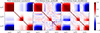Fig. 1. Correlation matrices of the τ statistics for different methods. The panels, from left to right, correspond to the analytical expressions from Eq. (18), jackknife resampling, and simulations, respectively.

Figure 2 shows the diagonal components of the covariance matrix for each method, including the contribution from the different terms appearing in Eq. (21) and the shot noise computed with TREECORR. We noted some discrepancy for τ₀ on large scales between the semi-analytical covariance and the one obtained with simulations.

This difference is not straightforward to explain, as the three methods to estimate the covariance are based on different hypotheses that can bias the estimation of the covariance. The simulation covariance, for example, does not contain the term ξ^γcξ^γb in Eq. (21) coming from galaxy-PSF correlations, as the simulations are generated without accounting for the correlation with the star sample. It is thus expected that the simulation covariance underestimates the variance. The jackknife covariance is sensitive to the way the sky is patched. It is even more important in our case since the galaxy and star catalogues have different footprints and number densities. As a result, the number of stars and galaxies is inhomogeneous between patches and could lead to a biased estimate of the covariance. The semi-analytical covariance relies on correlation functions measured on data. The lack of theory for the PSF-PSF and galaxy-PSF correlations cannot be circumvented, but the shear-shear correlation function could be estimated from a theory prescription. This would lower the variance estimated from the semi-analytical covariance, as the shape-shape correlation function measured on data contains the cosmological signal as well as any systematic bias (e.g. leakage bias). More precisely, Eq. (21) shows a contribution of the shear-shear correlation function with a rho statistic: ξ^γγξ^bc. The noisy and biased shear-shear correlation function measured on the data contains a leakage bias that tends to increase the estimated variance, thus biasing high the estimate of the cosmic variance ρ₊ term in Fig. 2. The cosmic variance ‘−’ is only weakly affected and remains negligible. The semi-analytical covariance matrix also relies on strong assumptions, such as a simple survey geometry or the Gaussianity of the fields, that cannot hold nor explain part of the discrepancy observed on large scales.

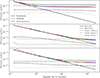Fig. 2. Diagonal component of the three τ statistics covariances for the different methods used to estimate the covariance. Upper panel: Diagonal of the τ0-τ0 covariance. Middle panel: Diagonal of the τ2-τ2 covariance. Lower panel: Diagonal of the τ5-τ5 covariance. Black and grey lines correspond to the individual contribution of each term in the covariance in Eq. (18). Small scales are shot noise dominated. We observed a good agreement between the three methods, and in particular, we validated the shot noise estimate of the semi-analytical covariance obtained from TREECORR (see Section 2.5.1).

We stress that the ellipticity error parameters (α, β, η) are nuisance parameters and that the goal is not to have a perfect estimate of their values but to build a prior on those parameters to marginalise the PSF systematics in the cosmological inference (see, e.g. Li et al. 2023a). Overestimating the variance using the semi-analytical prescription leads to conservative constraints on α, β, and η. Finally, we tested that using a ΛCDM theory prediction at a fiducial cosmology with CCL⁴ to estimate ξ^γγ in Eq. (21) lowered the discrepancy. Moreover, the high correlation between the angular scales in the τ statistics makes the inference very rigid, and this modification did not lead to a noticeable discrepancy in the constraints of the parameters and most importantly on the leakage bias of the shear-shear correlation function presented in Sect. 4.2.

Figure 3 presents constraints obtained on α, β, and η using the least-square method and MCMC. The values of the parameters are summarised in Table 1. We see that the contours obtained with the three covariance matrices are in very good agreement for both the least-squares and MCMC approaches. We observed a shift towards lower values of β when using the semi-analytical covariance matrix compared to the other two. This shift will appear in the systematic error presented in Section 4.2. We also observed a small shift of the predicted values of α and η using the semi-analytical covariance, resulting in the shift of the contour in the (α, η) plane. This shift occurs in the direction of the degeneracy between α and η, and as we show in the next section, it has no effect on the level of systematic error. The contours obtained using MCMC appear similar to the one obtained from least-squares. We study this similarity further in Section 4.3.

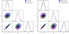Fig. 3. Constraints obtained on parameters Ω = (α, β, η)T of the PSF error model. Left panel: Constraints obtained using the least-square method. Right panel: Constraints obtained using MCMC.

Figure 4 shows the best-fit curves of the τ statistics for each method to estimate the covariance. We observed that the agreement between the three covariances is good and provides a convincing fit to the data. A slight discrepancy can be seen on large scales for τ₂. The reason for this is the high correlation between the three τ statistics on large scales, which prevents the model from perfectly fitting all three τ statistics at the same time.

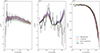Fig. 4. Observed data with error bars and best fit (solid line) of the τ statistics at the 68% confidence level (dashed lines) for the three different methods used to estimate the covariance matrix of the τ statistics. The τ statistics were estimated using parameters (α, β, η) sampled with least-squares. We note that τ2 and τ5 are multiplied by ϑ in the middle and right panels.

4.2. Comparison of the predicted level of systematics for the different covariance matrices

In the previous subsection, we described how the fitted values of α, β, and η are consistent between the different covariance matrices used for the τ statistics. There are, however, slight shifts in the contours, and it is therefore important to check whether those shifts yield significantly different estimates of the level of systematic error using Eq. (15). Figure 5 shows the level of systematic due to the PSF for the ‘+’ component of the two-point correlation function ξ₊^γγ(ϑ) using both the least-squares solution and MCMC. The error bars correspond to the 68% level of confidence. Using both methods, we observed that the systematic levels are in agreement, particularly on large scales. A slight difference can be observed on small scales between the three methods. This difference can be explained by the slight shift in the value of β between the three methods. Indeed, as can be seen in Figure 6, the level of systematics on small scales is sensitive to the value of β (see the lower panel). As a result, an offset in the estimated value of β will result in more or less systematics on those scales. However, the slight shift in α and η cannot be observed when looking at the level of systematics, ξ_PSF, sys.

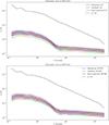Fig. 5. Level of systematic error for the different methods to estimate the covariance matrices. We show the confidence interval for the level of systematics at the 68% confidence level (dashed lines). Top panel: Using least-squares to estimate the parameters. Bottom panel: Using MCMC to estimate the parameters. The dotted-dashed line corresponds to the ξ+ two-point correlation function to which the level of systematics has to be compared.

From the contours in Figure 3, we observed that α and η are positively correlated. This correlation is expected because α corresponds to the leakage term e^p and η corresponds to the size residual. To make the latter a spin-2 quantity, it is multiplied by e^*, which due to the small size of the residuals also carries information on the leakage. The third panel of the Figure 6 shows that along this degeneracy in the (α, η) plane, the estimated level of systematics, ξ_PSF, sys, is similar. The upper panels of Figure 6 show that α and η mostly influence the level of systematics on large scales when their degeneracy in the (α, η) plane is not followed.

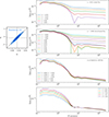Fig. 6. Dependency of the level of systematics on the parameters α, β, and η of the PSF error model. Upper panel: Dependency on η with α and β fixed. It follows the dotted line in the left panel. Middle upper panel: Dependency on α with β and η fixed. It follows the dash dotted line in the left panel. Middle lower panel: Dependency following the degeneracy (solid line in the left panel) in the (α, η) plane with β fixed. Lower panel: Dependency on β with α and η fixed.

A redefinition of the error model (15) is explored in Section 5.2. There, we show that it can break the degeneracy between α and η with no significant modification of the estimated level of systematic error, ξ_PSF, sys. Finally, we emphasise that the dependence on the systematic level drawn in this section might be survey specific, as it depends on the amplitude of the ρ statistics. As the choice of PSF model and shape measurement methods vary from one survey to the other, ρ statistics might show different amplitudes associated with the leakage or the residuals, thus leading to a different interpretation.Nevertheless, we deem it to be important to PSF systematics and their scale dependence, which we demonstrate here using UNIONS data and making use of ρ and τ statistics.

4.3. Comparison of the least-squares and MCMC methods

Here, we investigate the differences between the contours obtained using least-squares and MCMC. Figure 7 shows the constraints for α, β, and η, and Figure 8 shows the corresponding level of systematic error. We performed a comparison of the inference methods using the covariance matrix obtained from simulations. We observed that the contours are very similar, and the corresponding level of systematic error is in very good agreement. We underline, however, that the least-square method relies on a frequentist approach in the sense that the parameters are sampled by solving the least-square problem sampling a ρ and τ statistics realisation from their respective covariances. We stress that our work addresses the issue of covariance estimation for the τ statistics but not for the ρ statistics. In our case, we used the covariance matrix obtained from jackknife resampling to sample the ρ statistics and checked that the contours were not very sensitive to the noise in the covariance estimate. However, we observed differences in the size of the error bars compared to the method using least-squares, and therefore relying on the covariance estimate of the ρ statistics, and the method using MCMC. Least-squares and MCMC give similar results when using the semi-analytical or jackknife covariance matrices. The difference in the size of the error bars between MCMC and least-squares is more pronounced when using a jackknife covariance.

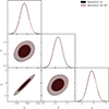Fig. 7. Constraints obtained on α, β, and η using least-squares (black) and MCMC (brown). The covariance used to perform the fit is from GLASS simulations.

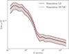Fig. 8. Level of systematics obtained using a covariance matrix computed from simulations for parameter estimation using least-squares (black) and MCMC (brown).

5. Discussion

5.1. A semi-analytical τ covariance for fast and accurate diagnostics

In the previous sections, we demonstrated that the semi-analytical covariance introduced in this work can provide a similarly precise estimate of the level of systematic error as when using a covariance computed from simulations or with jackknife resampling. Despite showing a larger χ² for the best-fit parameters than the other two methods, the semi-analytical covariance provides a similar fit to the data (See Figure 4) and contours consistent with the other two methods (See Figure 3). The main advantage of the semi-analytical covariance compared to simulations or jackknife resampling is its reduced computation time. It does not require simulations for each catalogue, and therefore allows one to save a significant amount of computation time and storage. This is particularly important in a tomographic analysis, where the size of the τ data vector and therefore the amount of simulations required to estimate the covariance can be very large. For example, the time required to compute the semi-analytical covariance matrix used in this paper on 48 cores of an Intel Xeon-G 5220R processor is 27 minutes, compared to 227 minutes when using jackknife resampling. Our analytical approach also explicitly contains cross-correlation terms between galaxies and stars that are not contained in the GLASS simulations. Moreover, it does not depend on the way the sky is patched, in contrast to jackknife resampling. It can also be used on small sky areas where jackknife resampling becomes complicated due to the small number of objects in each patch and the difficulty of finding a trade-off between the number of patches and the number of objects per patch. Our approach thus allows one to compute local estimates of PSF systematics and, for example, to compare the level of systematics in different patches of a survey. In a nutshell, the semi-analytical covariance for the τ statistics is a powerful tool to perform PSF diagnostics on several galaxy and star catalogues obtained with, for example, different signal-to-noise ratios or size cuts.

5.2. Towards a redefinition of the τ statistics

In Section 4.2, we shed light on the degeneracy between the leakage parameter α and the size residual η that appear with UNIONS data. This degeneracy is expected, as the size residual is multiplied by the ellipticity of stars e^* to yield a spin-2 field. This allows for spin consistency between all terms in Eq. (8), although the introduction of this parameter does not provide additional information (see e.g. Giblin et al. 2021; Zhang et al. 2023; Gatti et al. 2021). In this section, we redefine the ρ and τ statistics by replacing the e^* factor in front of the size residual with a projector on the tangential direction f such that

$$\begin{array}{c}\hfill {\stackrel{\sim }{e}}^{\mathrm{PSF},\mathrm{sys}}=\alpha e^{\mathrm{p}}+\beta \delta e^{\mathrm{p}}+\eta \delta {\stackrel{\sim }{T}}^{\mathrm{p}},\end{array}$$(36)

where $\delta {\stackrel{\sim }{T}}^{\mathrm{p}}=f(T^{\ast }-T^{\text{p}})/T^{\ast }$. The field, f, is implicitly defined with respect to the pairs such that when computing the ρ and τ correlations, only the tangential direction contributes at star positions and for a given polar angle ϕ. Thus, f reverts to the unit vector in the tangential direction, $f={\widehat{e}}_{\mathrm{t}}$. The correlation function between a spin-2 field a and the product of f with a scalar field s is therefore obtained as follows:

$$\begin{array}{cc}\hfill {\xi }_{\pm }^{a[fs]}(\vartheta )& =⟨a_t{f}_{t}s⟩(\vartheta )\pm {\displaystyle \underset{=0}{\underbrace{⟨a_{\times }{f}_{\times }s⟩(\vartheta )}}}\hfill \\ \hfill & =⟨a_{t}s⟩(\vartheta ).\hfill \end{array}$$(37)

The ‘+’ and ‘−’ components of the correlation function are thus degenerate and correspond to the correlation between the tangential component of the spin-2 field a at each object position with respect to the scalar field s, which corresponds to what we expect. The ρ and τ statistics involving the size residuals are redefined as well with

$$\begin{array}{c}\hfill {\stackrel{\sim }{\rho }}_3(\vartheta )=⟨\delta {\stackrel{\sim }{T}}^{\mathrm{p}}\delta {\stackrel{\sim }{T}}^{\mathrm{p}}⟩;{\stackrel{\sim }{\rho }}_4(\vartheta )=⟨\delta e^{\mathrm{p}}\delta {\stackrel{\sim }{T}}^{\mathrm{p}}⟩;{\stackrel{\sim }{\rho }}_5(\vartheta )=⟨e^{\mathrm{p}}\delta {\stackrel{\sim }{T}}^{\mathrm{p}}⟩,\end{array}$$(38)

and

$$\begin{array}{c}\hfill {\stackrel{\sim }{\tau }}_5(\vartheta )=⟨e\delta {\stackrel{\sim }{T}}^{\mathrm{p}}⟩.\end{array}$$(39)

With that, the two-point correlations ${\stackrel{\sim }{\rho }}_4,{\stackrel{\sim }{\rho }}_5$, and ${\stackrel{\sim }{\tau }}_5$ correspond to tangential ellipticity around stars weighted by δT, and ${\stackrel{\sim }{\rho }}_3$ is the δT scalar auto-correlation function. The term ${\stackrel{\sim }{e}}^{\text{PSF, sys}}$ is not a correctly defined spin-2 field, but the two-point correlators are well defined and allow one to decorrelate the information carried by α and η. Losing this property, ${\stackrel{\sim }{e}}^{\text{PSF, sys}}$ has the benefit of providing quantitative estimates of α and η that can be more easily compared between catalogues, as they respectively carry the information of leakage and size residuals only. In practice, we used the TREECORR KKCORRELATION class for ${\stackrel{\sim }{\rho }}_3$ and GKCORRELATION for ${\stackrel{\sim }{\rho }}_4,{\stackrel{\sim }{\rho }}_5$, and ${\stackrel{\sim }{\tau }}_5$, and we set δT as the scalar field ‘K’ for the correlation. With this new definition, ${\stackrel{\sim }{\tau }}_5$ provides a null test related to the quality of the size estimation of the PSF, whereas τ₅ carried information on both the size residual and the leakage due to the e^* factor. Figures 9 and 10 show that the $\stackrel{\sim }{\tau }$ statistics provide an accurate fit to the data and remove the degeneracy between the leakage parameter α and the size residuals parameter η. In the figures, ${\stackrel{\sim }{\tau }}_5$ is the only modified τ statistic, and it provides a null test to check if the size residuals contribute significantly to an additive bias. With our data, it seems to show that the leakage is the main contributor to the correlation between the shape of galaxies and stars, whereas the correlation with the size residuals is consistent with zero (see right panel in Fig. 9).

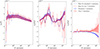Fig. 9. Best-fit model of the τ and $\stackrel{\sim }{\tau }$ statistics obtained using a least-squares sampling method. We show the 68% confidence region.

Fig. 10. Constraints obtained on α, β, and η using least-squares with the redefined $\stackrel{\sim }{\tau }$ statistics.

The covariance matrix of the $\stackrel{\sim }{\tau }$ statistics was estimated using jackknife resampling. Figure 11 shows that the level of systematics obtained with the $\stackrel{\sim }{\tau }$ statistics matches the one obtained from the standard τ statistics at the 68% confidence level. With the $\stackrel{\sim }{\tau }$ statistics, we are thus able to break the degeneracy between α and η by disentangling the information carried by τ₀ and τ₅. Hence, we advocate that $\stackrel{\sim }{\tau }$ statistics provide a more interpretable description of PSF systematics, particularly when the size residuals are not very small, and argue that it should be preferred over standard τ statistics when a strong degeneracy between α and η is observed. The semi-analytical covariance matrix introduced in Sect. 2.5 can be revised to compute the auto- and cross-correlations involving ${\stackrel{\sim }{\tau }}_5$. However, we leave this for future work.

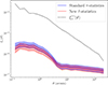Fig. 11. Level of systematics obtained using the least-squares sampling method with standard τ statistics and the redefined $\stackrel{\sim }{\tau }$ statistics (see Eq. (39)).

6. Conclusions

The goal of this paper is to provide a methodology to compute fast and accurate estimates of PSF systematics that pollute the two-point cosmic shear correlation function. To that end, we used the so-called ρ and τ statistics and developed a semi-analytical covariance of the τ statistics to obtain fast and accurate estimates of PSF systematics for a given catalogue of galaxies (Sect. 2.5). In addition, we estimated the PSF parameters as the exact solution of a least-square problem and explored the credible region of parameter space via sampling of the covariance matrices of the τ and ρ statistics.

We applied our methodology to UNIONS data, where the PSF was obtained with the data-driven PSF model MCCD (Section 3). We found a good agreement for our semi-analytical covariance with estimates using simulations and jackknife resampling (Sect. 4). We stress the comparatively low computation time to calculate the semi-analytical covariance matrix compared to jackknife or simulation-based estimates with acceptable low sampling noise. The speed-up is of the order of eight between the semi-analytical and jackknife covariance. We note that the semi-analytical covariance contains galaxy-PSF cross-correlation terms that are missing from state-of-the-art simulations.

The inferred PSF systematics parameters are in excellent agreement between all three covariance matrix inputs, even though with the semi-analytical covariance the reduced χ² value of the best-fit model is the highest of the three. We found excellent agreement of our least-square parameter estimation and exploration with MCMC sampling, at an order of three times lower computation time. The total gain in computing time using least-squares with the semi-analytical covariance over MCMC sampling using jackknife or simulations is a factor of 8.2.

We also observed that our analysis finds an important degeneracy between the parameter α, measuring the amplitude of the ‘PSF leakage’, and the parameter η associated with the size residuals of the PSF (Section 5). This degeneracy arises naturally, as the size residual is multiplied by the ellipticity of stars to yield a spin-2 field. We explored a redefinition of the τ statistics that considers the size residuals as a scalar field to disentangle the PSF systematics coming from PSF leakage and from the size residuals. We argue that even though the error model loses physical consistency, it allows results similar to the standard τ statistics to be recovered without the degeneracy in the (α, η) plane. In cases where this degeneracy appears, one should prefer the use of this redefinition to know whether leakage or size residuals dominate the PSF systematics. We also highlight that we only considered PSF second moments, whereas previous work have shown that fourth moments can carry significant information on PSF systematics that is not taken into account in our context (See e.g. Zhang et al. 2023, for more information). We emphasise that the mathematical framework to compute a semi-analytical covariance matrix with τ statistics extended to the fourth moment is analogous to the one introduced in this work and can be easily transposed if needed.

This work provides useful tools to perform the analysis of the ongoing UNIONS survey but also for future surveys (e.g. Euclid or LSST). The semi-analytical covariance can be a useful tool in the era of Stage IV large-scale structure surveys for performing fast PSF diagnostics on catalogues obtained either on different patches of the sky or with different cuts that could influence PSF systematics. It will be crucial to understand those systematics correctly, as the wide area coverage and increased depth of such surveys will likely yield statistical errors that are negligible compared to the systematics for the shear-shear two-point correlation function. In the context of the Euclid mission, it will also be a useful tool to validate the shape measurement algorithm and the PSF model. Finally, as soon as the analysis pipeline is frozen, it provides a useful estimate of the PSF systematics, which can be taken into account in the modelling when performing MCMC estimations of the cosmological parameters or calibrated for beforehand (Li et al. 2023b). This methodology will also be useful in a context where forward models become essential tools to validate analysis pipelines, such as for 3x2 point statistics (Amon et al. 2023), or to perform inference using simulation-based methods (von Wietersheim-Kramsta et al. 2025; Jeffrey et al. 2025; DES Collaboration 2024), where all systematics must be forward modelled correctly to avoid model misspecification and guarantee an unbiased inference (Cannon et al. 2022).

Data availability

For the sake of reproducible research, the figures shown in this work can be reproduced using the code available on the GitHub repository associated with the paper (https://github.com/sachaguer/tau_stats_paper). The repository contains the covariance matrices computed using simulations, jackknife resampling, and the analytical expressions, as well as the samples obtained from these matrices. Companion notebooks allow the user to create the figures from the provided data. The code used to compute the semi-analytical covariance matrix is publicly available on GitHub (https://github.com/martinkilbinger/shear_psf_leakage).

Acknowledgments

We are honoured and grateful for the opportunity of observing the Universe from Maunakea and Haleakala, which both have cultural, historical and natural significance in Hawaii. This work is based on data obtained as part of the Canada-France Imaging Survey, a CFHT large program of the National Research Council of Canada and the French Centre National de la Recherche Scientifique. Based on observations obtained with MegaPrime/MegaCam, a joint project of CFHT and CEA Saclay, at the Canada-France-Hawaii Telescope (CFHT) which is operated by the National Research Council (NRC) of Canada, the Institut National des Science de l’Univers (INSU) of the Centre National de la Recherche Scientifique (CNRS) of France, and the University of Hawaii. This research used the facilities of the Canadian Astronomy Data Centre operated by the National Research Council of Canada with the support of the Canadian Space Agency. This research is based in part on data collected at Subaru Telescope, which is operated by the National Astronomical Observatory of Japan. Pan-STARRS is a project of the Institute for Astronomy of the University of Hawaii, and is supported by the NASA SSO Near Earth Observation Program under grants 80NSSC18K0971, NNX14AM74G, NNX12AR65G, NNX13AQ47G, NNX08AR22G, 80NSSC21K1572 and by the State of Hawaii. LB is supported by the PRIN 2022 project EMC2 – Euclid Mission Cluster Cosmology: unlock the full cosmological utility of the Euclid photometric cluster catalog (code no. J53D23001620006). This work was made possible by utilising the CANDIDE cluster at the Institut d’Astrophysique de Paris. The cluster was funded through grants from the PNCG, CNES, DIM-ACAV, the Euclid Consortium, and the Danish National Research Foundation Cosmic Dawn Center (DNRF140). It is maintained by Stephane Rouberol. We also gratefully acknowledge support from the CNRS/IN2P3 Computing Center (Lyon – France) for providing computing and data-processing resources needed for this work. H. Hildebrandt is supported by a DFG Heisenberg grant (Hi 1495/5-1), the DFG Collaborative Research Center SFB1491, an ERC Consolidator Grant (No. 770935), and the DLR project 50QE2305.

References

Appendix A: Derivation of the two-point spin-2 correlators

Here we detail the derivation of the relations Eq. (6). We first define the parity-violating correlation function ξ_×, which mixes tangential and cross components. Another parity-variant function exists, which we call ξ_*. Their expressions are

$$\begin{array}{cc}\hfill {\xi }_{\ast }^{\mathit{ab}}(\vartheta )& =-\langle a_{\mathrm{t}}{b}_{\times }\rangle (\vartheta )+\langle a_{\times }{b}_{\mathrm{t}}\rangle (\vartheta )\hfill \\ \hfill & =-\langle a_1{b}_2\rangle (\vartheta )+\langle a_2{b}_1\rangle (\vartheta )\hfill \\ \hfill & =\mathfrak{I}\left[\langle a{b}^{\ast }\rangle (\vartheta )\right];\hfill \\ \hfill {\xi }_{\times }^{\mathit{ab}}(\vartheta )& =\langle a_{\mathrm{t}}{b}_{\times }\rangle (\vartheta )+\langle a_{\times }{b}_{\mathrm{t}}\rangle (\vartheta )\hfill \\ \hfill & =\langle [-\left(a_1{b}_1\right)(\mathit{\vartheta })+\left(a_2{b}_2\right)(\mathit{\vartheta })]sin4\varphi \rangle \hfill \\ \hfill & +\langle [\left(a_1{b}_2\right)(\mathit{\vartheta })+\left(a_2{b}_1\right)(\mathit{\vartheta })]cos4\varphi \rangle \hfill \\ \hfill & =\mathfrak{I}\langle \left(ab\right)(\mathit{\vartheta })e^{-4\mathrm{i}\varphi }\rangle .\hfill \end{array}$$(A.1)

The four real-valued correlation functions defined in Eqs. (3) and (A.1) can be combined into two complex correlation functions between the field a_t + ia_× = aexp(−2iϕ) and the field b_t + ib_× and its complex conjugate b_t − ib_×, respectively; these fields are well-defined given a direction with polar angle ϕ. The two complex correlation functions ⟨ab^*⟩(ϑ) and ⟨(ab)(ϑ)exp(−4iϕ)⟩ were introduced in Jarvis et al. (2004) as the natural components of the shear two-point correlation function. Combining Eq. (2) into a complex quantity $\stackrel{\sim }{a}=a_{\mathrm{t}}+\mathrm{i}{a}_{\times }$, we can write these natural components as

$$\begin{array}{cc}\hfill {\xi }_{+}^{\mathit{ab}}(\vartheta )+\mathrm{i}{\xi }_{\ast }^{\mathit{ab}}(\vartheta )& =\langle a{b}^{\ast }\rangle (\vartheta )=\langle \stackrel{\sim }{a}{\stackrel{\sim }{b}}^{\ast }\rangle (\vartheta );\hfill \\ \hfill {\xi }_{-}^{\mathit{ab}}(\vartheta )+\mathrm{i}{\xi }_{\times }^{\mathit{ab}}(\vartheta )& =\langle ab{\mathrm{e}}^{-4\mathrm{i}\varphi }\rangle (\vartheta )=\langle \stackrel{\sim }{a}\stackrel{\sim }{b}\rangle (\vartheta ).\hfill \end{array}$$(A.2)

Getting back to Eqs. (6), for the first two equal component equations, we expanded

$$\begin{array}{c}\hfill \langle a_{i\alpha }{b}_{j\alpha }\rangle =\frac{1}{2}(\langle a_{i\alpha }{b}_{j\alpha }\rangle +\langle a_{i\beta }{b}_{j\beta }\rangle )+\frac{1}{2}[\langle a_{i\alpha }{b}_{j\alpha }\rangle -\langle a_{i\beta }{b}_{j\beta }\rangle ].\end{array}$$(A.3)

With α ≠ β sum in the first round bracket is ξ₊^ab(ϑ_ij). For the difference in the second bracket we note that when forming the combination ξ₋^ab(ϑ_ij)cos4ϕ_ij − ξ_×(ϑ_ij)sin4ϕ_ij all mixed-component terms vanish, leaving the difference of the products of equal components. The difference between α = 1 (and thus β = 2) and α = 2 is a minus sign, and we recover the first two equations of Eq. (6).

For the third and fourth mixed-component equations, we expanded in a similar manner:

$$\begin{array}{c}\hfill \langle a_{i\alpha }{b}_{j\beta }\rangle =\frac{1}{2}(\langle a_{i\alpha }{b}_{j\beta }\rangle +\langle a_{i\beta }{b}_{j\alpha }\rangle )+\frac{1}{2}(\langle a_{i\alpha }{b}_{j\beta }\rangle -\langle a_{i\beta }{b}_{j\alpha }\rangle ).\end{array}$$(A.4)

The second bracket is ξ_*(ϑ_ij) if α = 1, and with an additional minus sign for α = 2. The first term is symmetrical in α and β, and equal to ξ₋^ab(ϑ_ij)sin4ϕ_ij + ξ_×^ab(ϑ_ij)cos4ϕ_ij.

Appendix B: Gaussianity test of the τ statistics

One of the main hypothesis underlying the expression of the semi-analytical covariance matrix in Eq. (18) is that the fields considered to compute the τ statistics are Gaussian. It allows us to apply Wick’s theorem in Eq. (19) to expand the four-point correlators in a sum of two-point correlators that we are able to measure easily. To test this hypothesis, we apply the methodology of Sellentin & Heavens (2018) with similar notations. That work introduced three ‘transcovariance’ matrices to detect non-Gaussianities in the likelihood. These matrices help to examine whether the sum, the ratio, and the product of two independently drawn samples of the data are distributed differently from a Gaussian distribution, a Cauchy distribution, and two linearly superposed χ₁²-random variables, respectively. Those distributions are expected for samples drawn from independent unit Gaussians. As we simulated 300 independent realisations of the τ statistics using GLASS (see Sect. 3.2), we can use them to compute the transcovariance matrices of the τ statistics.

We note with x_i^e the i^th realisation of element e of the τ statistics data vector (=e^th row in Eq. (13)). Our goal is to test whether two τ values x^e and x^f pass the Gaussianity tests. To that end, we first remove the Gaussian correlation between both variables with a mean-subtraction and whitening step. The whitening step is applied to the two-dimensional covariance matrix between x^e and x^f, C_αβ = ⟨x^αx^β⟩, for α, β = 1, 2, with x¹ = x^e, x² = x^f. If the data was indeed Gaussian, the sum, ratio and product of the samples should have the distributions as stated above. To test if the distributions match, we use the N = 300 simulated and whitened τ statistics to estimate the sum, ratio and product for each pair (e, f) of data vector entry. We then bin their distribution into B histogram values ℋ_b, b = 1…B. The distance from the histogram to the expected distribution is computed using the so-called Mean Integrated Squared Errors (MISE). As an example, for the sum

$$\begin{array}{c}\hfill s_i^{e,f}=x_i^e+x_i^f,\end{array}$$(B.1)

the target distribution is a Gaussian with a variance of two. It allows the ‘transcovariance’ for the sum to be defined:

$$\begin{array}{c}\hfill {\mathbf{S}}_{e,f}^{+}=\frac{1}{B}{\displaystyle \sum _{b=1}^B}{[{\mathcal{H}}_b(s_i^{e,f})-\mathcal{G}(0,2)]}^2.\end{array}$$(B.2)

In the limit where the number of samples N and the number of bins B go to infinity, the weak law of great numbers ensures the convergence of the histogram to 𝒢(0, 2) if the data only contains Gaussian correlations. In that case, S⁺ should be null. One can define in the same way transcovariance matrices S^* and S^÷ for the product and the ratio of the samples. In the case of the product, the probability distribution function has no closed form as the two χ₁² linearly superposed are not independent. It is however easy to sample from this distribution and therefore we will compute the MISE for S^* using a histogram sampled from the correct distribution. Fig. B.1 shows those transcovariance matrices obtained using GLASS simulations. Each matrix coefficient (e, f) corresponds to the amount of non-Gaussianity in the correlation between x^e and x^f. Because we only have access to a finite amount of samples N and number of bins B, the estimate of the total non-Gaussian contamination ϵ_e^tot, + is polluted by a shot noise. To characterise the noise, we draw N Gaussian distributed samples with the same covariance as our dataset. From those N Gaussian distributed samples, we compute calibration matrices S_cal⁺, S_cal^* and S_cal^÷. In particular, this calibration set allows us to choose the number of bins to compute the histogram that minimises the amount of structure observed in the transcovariances S^* and S^÷ as their distribution is peaked and can thus introduce spurious structures in the Gaussian samples transcovariances.

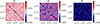Fig. B.1. Transcovariance matrices S+, S* and S÷ obtained from the τ statistics samples from GLASS simulations. Each matrix coefficient (e, f) measures the amount of non-Gaussianity in the correlation between the e-th and the f-th entry of the data vector.

We can therefore use those matrices to define the total non-Gaussian contamination of the e-th data point as the sum over the column of the transcovariance matrix, for example, for the sum

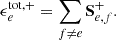$$\begin{array}{c}\hfill {ϵ}_e^{\mathrm{tot},+}={\displaystyle \sum _{f\ne e}}{\mathbf{S}}_{e,f}^{+}.\end{array}$$(B.3)

One can then define a threshold, for the total non-Gaussian contamination defined in Eq. (B.3), beyond which the distribution of the data point is considered non-Gaussian. To characterise if this value is significant and points at non-Gaussian correlation, it has to be compared with the shot noise due to the limited amount of samples N and bins B computed using data sampled from a multivariate Gaussian distribution as described above. Fig. B.2 shows the total non-Gaussian contamination for each data vector entry against the shot noise computed on the Gaussian samples. We note that the contamination obtained is noisier when using the product or ratio transcovariance matrices as the Cauchy and χ₁² are more peaked. We see that the total non-Gaussian contamination is not significantly higher than the shot noise and we thus do not detect deviations from Gaussianity in the distribution of the data. The Gaussian approximation used in the analysis in Sect. 2.4 is thus justified.

Fig. B.2. Total non-Gaussianity contamination at each entry of the data vector for each test. The blue region represents the shot noise due to the finite number of samples N and the limited amount of bins B. The red lines show the non-Gaussianity obtained for the τ statistics that are not significantly above the shot noise.

All Tables

References

- Akeson, R., Armus, L., Bachelet, E., et al. 2019, arXiv e-prints [arXiv:1902.05569] [Google Scholar]
- Amon, A., Robertson, N. C., Miyatake, H., et al. 2023, MNRAS, 518, 477 [Google Scholar]
- Asgari, M., Lin, C.-A., Joachimi, B., et al. 2021, A&A, 645, A104 [NASA ADS] [CrossRef] [EDP Sciences] [Google Scholar]
- Bartelmann, M., & Schneider, P. 2001, Phys. Rep., 340, 297 [Google Scholar]
- Bertin, E. 2011, ASP Conf. Ser., 442, 435 [Google Scholar]
- Cannon, P., Ward, D., & Schmon, S. M. 2022, arXiv e-prints [arXiv:2209.01845] [Google Scholar]
- Dalal, R., Li, X., Nicola, A., et al. 2023, Phys. Rev. D, 108, 123519 [CrossRef] [Google Scholar]
- DES Collaboration (Amon, A., et al.) 2022, Phys. Rev. D, 105, 023514 [NASA ADS] [CrossRef] [Google Scholar]
- DES Collaboration (Gatti, M., et al.) 2024, Phys. Rev. D, 109, 063534 [NASA ADS] [CrossRef] [Google Scholar]
- Farrens, S., Guinot, A., Kilbinger, M., et al. 2022, A&A, 664, A141 [NASA ADS] [CrossRef] [EDP Sciences] [Google Scholar]
- Foreman-Mackey, D., Hogg, D. W., Lang, D., & Goodman, J. 2013, PASP, 125, 306 [Google Scholar]
- Friedrich, O., Seitz, S., Eifler, T. F., & Gruen, D. 2016, MNRAS, 456, 2662 [NASA ADS] [CrossRef] [Google Scholar]
- Gatti, M., Sheldon, E., Amon, A., et al. 2021, MNRAS, 504, 4312 [NASA ADS] [CrossRef] [Google Scholar]
- Giblin, B., Heymans, C., Asgari, M., et al. 2021, A&A, 645, A105 [NASA ADS] [CrossRef] [EDP Sciences] [Google Scholar]
- Guinot, A., Kilbinger, M., Farrens, S., et al. 2022, A&A, 666, A162 [NASA ADS] [CrossRef] [EDP Sciences] [Google Scholar]
- Gwyn, S., McConnachie, A. W., Cuillandre, J. C., et al. 2025, AJ, submitted [arXiv:2503.13783] [Google Scholar]
- Hamana, T., Shirasaki, M., Miyazaki, S., et al. 2020, PASJ, 72, 16 [Google Scholar]
- Heymans, C., White, M., Heavens, A., Vale, C., & van Waerbeke, L. 2006, MNRAS, 371, 750 [Google Scholar]
- Heymans, C., van Waerbeke, L., Miller, L., et al. 2012, MNRAS, 427, 146 [NASA ADS] [CrossRef] [Google Scholar]
- Huff, E., & Mandelbaum, R. 2017, ApJ, submitted [arXiv:1702.02600] [Google Scholar]
- Ibata, R. A., McConnachie, A., Cuillandre, J.-C., et al. 2017, ApJ, 848, 128 [Google Scholar]
- Ivezić, Ž., Kahn, S. M., Tyson, J. A., et al. 2019, ApJ, 873, 111 [Google Scholar]
- Jarvis, M., Bernstein, G., & Jain, B. 2004, MNRAS, 352, 338 [Google Scholar]
- Jarvis, M., Sheldon, E., Zuntz, J., et al. 2016, MNRAS, 460, 2245 [Google Scholar]
- Jeffrey, N., Whiteway, L., Gatti, M., et al. 2025, MNRAS, 536, 1303 [Google Scholar]
- Kaiser, N., Squires, G., & Broadhurst, T. 1995, ApJ, 449, 460 [Google Scholar]
- Kilbinger, M. 2015, Rep. Progr. Phys., 78, 086901 [Google Scholar]
- Kilbinger, M., & Schneider, P. 2004, A&A, 413, 465 [NASA ADS] [CrossRef] [EDP Sciences] [Google Scholar]
- Kilbinger, M., Ishida, E. E. O., & Cisewski-Kehe, J. 2023, Astron. Comput., 43, 100705 [Google Scholar]
- Laureijs, R., Amiaux, J., Arduini, S., et al. 2011, arXiv e-prints [arXiv:1110.3193] [Google Scholar]
- Li, X., Zhang, T., Sugiyama, S., et al. 2023a, Phys. Rev. D, 108, 123518 [CrossRef] [Google Scholar]
- Li, S.-S., Kuijken, K., Hoekstra, H., et al. 2023b, A&A, 670, A100 [NASA ADS] [CrossRef] [EDP Sciences] [Google Scholar]
- Li, Q., Kilbinger, M., Luo, W., et al. 2024, ApJ, 969, L25 [Google Scholar]
- Liaudat, T., Bonnin, J., Starck, J.-L., et al. 2021, A&A, 646, A27 [NASA ADS] [CrossRef] [EDP Sciences] [Google Scholar]
- Mandelbaum, R. 2018, ARA&A, 56, 393 [Google Scholar]
- Mellier, Y., Abdurro’uf, A., Barroso, J. A. A., et al. 2025, A&A, 697, A1 [Google Scholar]
- Paulin-Henriksson, S., Amara, A., Voigt, L., Refregier, A., & Bridle, S. L. 2008, A&A, 484, 67 [NASA ADS] [CrossRef] [EDP Sciences] [Google Scholar]
- Rowe, B. 2010, MNRAS, 404, 350 [NASA ADS] [Google Scholar]
- Schneider, P., Van Waerbeke, L., Kilbinger, M., & Mellier, Y. 2002, A&A, 396, 1 [NASA ADS] [CrossRef] [EDP Sciences] [Google Scholar]
- Schneider, P., Van Waerbeke, L., & Mellier, Y. 2002, A&A, 389, 729 [NASA ADS] [CrossRef] [EDP Sciences] [Google Scholar]
- Sellentin, E., & Heavens, A. F. 2018, MNRAS, 473, 2355 [NASA ADS] [CrossRef] [Google Scholar]
- Sheldon, E. S., & Huff, E. M. 2017, ApJ, 841, 24 [NASA ADS] [CrossRef] [Google Scholar]
- Tessore, N., Loureiro, A., Joachimi, B., von Wietersheim-Kramsta, M., & Jeffrey, N. 2023, OpJA, 6, https://doi.org/10.21105/astro.2302.01942 [Google Scholar]
- Virtanen, P., Gommers, R., Oliphant, T. E., et al. 2020, Nat. Methods, 17, 261 [Google Scholar]
- von Wietersheim-Kramsta, M., Lin, K., Tessore, N., et al. 2025, A&A, 694, A223 [NASA ADS] [CrossRef] [EDP Sciences] [Google Scholar]
- Zhang, T., Li, X., Dalal, R., et al. 2023, MNRAS, 525, 2441 [Google Scholar]
- Zhang, Z., Kilbinger, M., Peters, F. H., et al. 2024, A&A, 691, A75 [NASA ADS] [CrossRef] [EDP Sciences] [Google Scholar]