| Issue |
A&A
Volume 700, August 2025
|
|
|---|---|---|
| Article Number | A252 | |
| Number of page(s) | 15 | |
| Section | Extragalactic astronomy | |
| DOI | https://doi.org/10.1051/0004-6361/202553878 | |
| Published online | 26 August 2025 | |
Self-consistent population synthesis of active galactic nuclei from observational constraints in the X-rays
1
Department of Astronomy, University of Geneva, 1290 Versoix, Switzerland
2
Instituto de Estudios Astrofísicos, Universidad Diego Portales, Chile
3
Kavli Institute for Astronomy and Astrophysics, Peking University, Beijing 100871, China
⋆ Corresponding author: This email address is being protected from spambots. You need JavaScript enabled to view it.
Received:
24
January
2025
Accepted:
16
June
2025
Abstract
The cosmic X-ray background (CXB) is produced by the emission of unresolved active galactic nuclei (AGNs), thus providing key information about the properties of the primary and reprocessed X-ray emission components of the AGN population. Equally important are studies of individual sources that provide additional constraints on the properties of AGNs, such as their luminosity and obscuration. Until now, these constraints have not been self-consistently addressed by intrinsically linking emission, absorption, and reflection. Here, we performed numerical simulations with the ray-tracing code REFLEX, which allows us to self-consistently model the X-ray emission of AGNs with flexible geometries for the circumnuclear medium. Using the REFLEX-simulated emission of an AGN population, we attempted to simultaneously reproduce the CXB and absorption properties measured in the X-rays, namely the observed fraction of NH in bins of log(NH) and the fraction of absorbed AGNs, including their redshift and luminosity evolution. We sampled an intrinsic X-ray-luminosity function and constructed gradually more complex, physically motivated geometrical models. We examined how well each model can match all observational constraints using a simulation-based inference (SBI) approach. We find that, while the simple unification model can reproduce the CXB, a luminosity-dependent dusty torus is needed to reproduce the absorption properties. When adding an accretion disc, the model best matches all constraints simultaneously. Our synthetic population is able to reproduce the dependence of the covering factor on luminosity, the AGN number counts from several surveys, and the observed correlation between reflection and obscuration. Finally, we derived an intrinsic Compton-thick fraction of 21 ± 7%, which is consistent with local observations.
Key words: galaxies: active / X-rays: diffuse background / X-rays: galaxies
© The Authors 2025
 Open Access article, published by EDP Sciences, under the terms of the Creative Commons Attribution License (https://creativecommons.org/licenses/by/4.0), which permits unrestricted use, distribution, and reproduction in any medium, provided the original work is properly cited.
This article is published in open access under the Subscribe to Open model. This email address is being protected from spambots. You need JavaScript enabled to view it. to support open access publication.
1. Introduction
Supermassive black holes (SMBHs) at the cores of galaxies are the engines of active galactic nuclei (AGNs) during an accreting phase. The SMBHs are closely linked to essential properties of their host galaxies, including mass, velocity dispersion, and luminosity (e.g. Magorrian et al. 1998; Gebhardt et al. 2000; Kormendy & Ho 2013). Such correlations hint at the potential for SMBHs to regulate star formation rates and play a significant role in galaxy evolution. To comprehensively probe the evolution of SMBHs, AGN demographics have been examined through population studies, allowing us to build their luminosity function (e.g. Ueda et al. 2014; Aird et al. 2015; Ananna et al. 2019) and other properties such as the black-hole mass function and Eddington-ratio distribution function.
X-ray radiation is a universal feature of AGNs that typically outshines the emission of the host galaxy (e.g. Brandt & Alexander 2015). Furthermore, X-ray observations are very efficient for detecting obscured AGNs, as X-ray photons can penetrate the high column density of the surrounding dusty material, thus allowing us to study the innermost regions of AGNs. The primary X-ray emission is attributed to the inverse Comptonisation of accretion-disc photons in a hot corona close to the SMBH (e.g. Haardt & Maraschi 1991), while reprocessed components come from reflection on the circumnuclear material (e.g. Pounds et al. 1990; Ghisellini et al. 1994). The circumnuclear material is thought to be in the form of a dusty torus (see Hickox & Alexander 2018 for an overview) and acts as an absorber and reflector at the same time, while other dense structures such as the accretion disc can also act as reflectors. The integrated emission from the AGN population is imprinted on the cosmic X-ray background (CXB; e.g. Brandt & Yang 2022). A clear peak in the CXB spectrum is observed between 20 − 30 keV, which is attributed to the X-ray radiation reflected on the circumnuclear material. The CXB is often used as one of the constraints for AGN population-synthesis models (e.g. Gilli et al. 2007; Akylas et al. 2012; Ueda et al. 2014; Ananna et al. 2019); however, it can be reproduced by different AGN populations, for instance by assuming different AGN spectral features, the shape of the X-ray luminosity function (XLF), the intrinsic neutral hydrogen column-density (NH) distribution, and the fraction of Compton-thick (CT) AGNs (which we define as the fraction of AGNs with NH ≥ 1024 cm−2), as demonstrated in Treister et al. (2009), Akylas et al. (2012), and Ananna et al. (2019). Some degeneracy between these parameters could be lifted by using AGN number counts obtained in X-ray surveys (e.g. Ueda et al. 2014; Aird et al. 2015; Ananna et al. 2019).
X-ray surveys of AGNs also offer insights into their absorption properties, which strongly affect the emission from AGNs and thus the modelling of the CXB. The fraction of absorbed AGNs (usually defined as the fraction of AGNs with NH ≥1022 cm−2) has been consistently found to be anti-correlated with luminosity (e.g. Lawrence 1991; Ueda et al. 2003; Hasinger 2008; Ueda et al. 2014; Aird et al. 2015; Buchner et al. 2015), suggesting that there are intrinsic physical differences between the populations of obscured and unobscured AGNs. The intrinsic fraction of CT AGNs is still debated, with previous studies finding values from 10 to 50% (e.g. Brightman & Nandra 2011; Akylas et al. 2012; Ueda et al. 2014; Ricci et al. 2015; Ananna et al. 2019). As the CXB peak at 20 − 30 keV can be reproduced by either a high fraction of CT AGNs or stronger reflected X-ray emission from all AGNs, the amount of reflection must be anti-correlated with the fraction of CT AGNs. Studies with stronger reflection components find a CT fraction as low as 10% (e.g. Treister et al. 2009; Ricci et al. 2011), while the most recent population synthesis of AGNs in Ananna et al. (2019), which is able to simultaneously reproduce the CXB and AGN number counts from multiple X-ray surveys, predicts an intrinsic CT fraction of 56 ± 7% for z ≲ 1.
An important caveat of all previous studies is that the absorption of AGNs is assumed and is not physically linked with any other AGN properties. Until now, X-ray observables concerning the absorption properties of AGNs, such as the observed column-density distribution and the dependence of the absorbed fraction on X-ray luminosity and redshift, have not been self-consistently addressed by physically linking obscuration and reflection. In this study, we create a fully self-consistent population-synthesis model of AGNs, where the X-ray obscuration and reflection are linked through the distribution of matter. In order to do so, we carried out numerical simulations using the ray-tracing code REFLEX (Paltani & Ricci 2017), which allows us to simulate the X-ray emission from AGNs with different geometries. We sampled an intrinsic X-ray-luminosity function to create a synthetic AGN population and used gradually more complex and physically motivated geometrical models. With each model, we attempted to reproduce the CXB and the observed absorption properties. We used a simulation-based inference approach (Tejero-Cantero et al. 2020; Greenberg et al. 2019) to compare the models to the observations and infer the model parameters that best match all constraints simultaneously. Finally, we examined the luminosity dependence of absorption, the AGN number counts at different energy bands, the reflection-obscuration correlation, and the impact of galactic obscuration on our population, and we derived the intrinsic CT fraction of the AGN population. Throughout this paper, all logarithmic values (log) refer to logarithms with base 10, and we adopted the following cosmological parameters: H0 = 70 km s−1 Mpc−1, Ωm = 0.3, and ΩΛ = 0.7.
2. X-ray observational constraints
To constrain the geometrical and physical properties of the AGN population, we had to gather several observational AGN properties. In Fig. 1, we show the X-ray observations used as constraints in this work, and we describe each of them in this section. The constraints are the CXB and several absorption properties from studies of X-ray surveys, namely the observed NH distribution and the dependence of the observed fraction of absorbed AGNs on observed X-ray luminosity and on redshift. We chose observed properties because the intrinsic ones depend on the assumptions made in other papers. Instead, we applied the selection function of each survey on our synthetic population.
 |
Fig. 1. X-ray observables used as constraints in this work. From the left: CXB measured by Chandra (cyan; Cappelluti et al. 2017), INTEGRAL (red; Churazov et al. 2007), RXTE (magenta; Revnivtsev et al. 2003), Swift/BAT (orange; Ajello et al. 2008), and Swift/XRT (blue; Moretti et al. 2009). The observed NH distribution of 731 AGNs in the 70-month Swift/BAT catalogue, detected in the 14–195 keV range, from Ricci et al. (2017a). The point with the dashed error bars represents the sum of the first two bins used in this work (see Sect. 2.2 for more information). The absorbed fraction of 1290 AGNs from multiple surveys in the 2–10 keV range is shown as a function of observed luminosity and as a function of redshift from Hasinger (2008). |
2.1. Cosmic X-ray background
The CXB is formed by the integrated emission of all AGN across cosmic time (see Brandt & Yang 2022 for an overview). As our first constraint, we use some of the most recent measurements of the CXB, comprehensively covering our target energy range, obtained from five instruments: Chandra, INTEGRAL (JEM-X, IBIS/ISGRI, SPI), RXTE/PCA, Swift/BAT and Swift/XRT (Cappelluti et al. 2017; Churazov et al. 2007; Revnivtsev et al. 2003; Ajello et al. 2008; Moretti et al. 2009; Fig. 1 top). All measurements find the CXB spectral index to be ∼1.4 below 10 keV. Any normalisation discrepancies between data sets may mostly be the result of inaccurate cross-calibration of spectra, unclear instrumental backgrounds, and cosmic variance (e.g. Moretti et al. 2009). We note the pioneering role of the HEAO-1 mission in the discovery and early characterisation of the CXB shape (Gruber et al. 1999). The statistical disagreement in normalisation between HEAO-1 and our chosen measurements is well documented and discussed in the literature (see, e.g. Churazov et al. 2007; Ajello et al. 2008; Moretti et al. 2009, and references therein). We considered the energy range 2–100 keV, as at E > 100 keV there is a significant contribution from blazars (e.g. Draper & Ballantyne 2009), and at E < 2 keV the AGN emission becomes quite complex because of absorption, soft-excess emission, and non-negligible contribution from galaxies (e.g. Cappelluti et al. 2012).
2.2. Absorption properties
2.2.1. Column-density distribution
The second constraint is the observed line-of-sight NH distribution of local (median redshift z = 0.0367) AGNs from Ricci et al. (2017a, hereafter R17). Their sample includes 731 non-blazar AGNs detected in the 14–195 keV energy band in the Swift/BAT 70-month all-sky survey. Being less biased against high- NH AGNs, it consists of ∼50% obscured AGN. The hard X-ray sensitivity of BAT allows us to investigate the distribution of absorption up to the CT regime, albeit with significant selection bias against CT AGN.
The NH distribution presented in R17 shows some evidence of bimodality with the highest peak for log(NH/cm−2)≤21 and the secondary in the log(NH/cm−2) = 23–24 bin (see Fig. 1, bottom left). The R17 distribution is largely consistent with NuSTAR observations in the 8–24 keV band, which also show two peaks at the same NH (e.g. Zappacosta et al. 2018). This bimodality suggests that the obscuration may be caused by different structures, possibly due to the plane of the galaxy hosting the AGN at lower NH and due to the denser circumnuclear material at higher NH (e.g. Paltani et al. 2008). Considering the purpose of this study, we do not model the host galaxy, resulting in a lack of mildly obscured (NH < 1022 cm−2) AGNs. Hence, we compared the number of simulated unobscured objects to all AGNs with NH < 1022 cm−2, assuming galactic column densities of log(NH/cm−2) < 22 (e.g. Güver & Özel 2009).
2.2.2. Fraction of absorbed AGNs
The last two constraints for this work are the observed fraction of absorbed AGNs as a function of the observed X-ray luminosity and as a function of redshift from Hasinger (2008; hereafter H08). In H08, 1290 AGNs detected in the 2–10 keV range from ten independent samples (summarised in Table 1 in their paper) are classified as type I (unabsorbed) or type II (absorbed) by combining optical spectroscopy and X-ray-hardness ratios. Optical/UV broad lines are used to classify sources into broad-line AGNs and narrow-line AGNs. The distinction found between the two classes corresponds to NH ≈ 3 × 1021 cm−2, above which only narrow lines are observable. Thus, for the calculation of the absorbed fraction, we considered the AGNs with log(NH/cm−2) > 21.5 [instead of the usual log(NH/cm−2) > 22] as absorbed in order to ensure a meaningful comparison with the H08 results.
In H08, the fraction of absorbed AGNs is found to decrease with increasing logarithmic luminosity with a slope of −0.226 ± 0.014 (fitted with a linear function) for log(LX/ erg s−1) ≥ 42. The presence of the anti-correlation has been confirmed by multiple studies carried out in the last three decades (e.g. Lawrence 1991; Ueda et al. 2003, 2014; Aird et al. 2015; Buchner et al. 2015). At the same time, in H08, the fraction of absorbed AGNs is found to increase with redshift as (1 + z)0.48 over the 0–3.2 redshift range at fixed luminosity. Such evolution was confirmed in later studies (Ueda et al. 2014; Aird et al. 2015; Liu et al. 2017; Iwasawa et al. 2020). Here, however, we considered the fraction integrated over the entire range of luminosity to avoid larger uncertainties caused by the low number of sources when the samples are divided into luminosity bins. In this case, the dependence of the fraction of absorbed AGNs on redshift is flat (Fig. 1 bottom right).
We opted for H08 instead of the more recent works cited above because it provides the absorbed fraction across broad luminosity and redshift ranges, in addition to using observed X-ray luminosities. This reduces the uncertainties that can arise from dividing into narrow bins with limited detected sources and avoids the additional assumptions made in other studies to infer intrinsic luminosities. Moreover, this is a consistent (as some studies do not provide the absorbed fraction as functions of both luminosity and redshift) and sufficient (as we do not expect that our simplistic models can explain all detailed features) set of constraints. Finally, in contrast to R17, the H08 sample contains both local and high redshift AGNs, meaning that our synthetic population has to be able to simultaneously match the absorption properties of AGNs detected at different redshifts as well as in different energy ranges (2–10 keV and 14–195 keV).
3. Modelling of the AGN population
We sought to create a self-consistent synthetic population of AGNs that can simultaneously reproduce the CXB and the observed absorption properties of AGNs. In our work, we looked for the geometrical model to best match the observables. In this section, we present the tools, models, and assumptions that we used to create the synthetic AGN population and simulate their emission.
3.1. RefleX
We used the ray-tracing code REFLEX1 (Paltani & Ricci 2017) to self-consistently simulate the X-ray emission of AGNs with different geometries. REFLEX performs realistic propagation of X-ray (0.1-1 MeV) photons through the circumnuclear material of AGNs using Monte Carlo methods. Arbitrary geometries with spatially varying composition and density can be selected by the user. Moreover, the geometry and emission spectrum of the X-ray source can also be selected. The most important physical processes in the X-rays are implemented, namely Compton and Rayleigh scattering, photoelectric absorption, and fluorescence. In REFLEX 3.0 (Ricci & Paltani 2023), dust absorption and scattering is also included following the Milky Way model from Draine (2003). We used the latest version of REFLEX to generate spectra at specific inclinations and calculate fluxes in selected energy bands.
3.2. X-ray luminosity function
To create a population of AGNs for our simulations, we needed an X-ray luminosity function, which provides the AGN number density in Mpc−3 dex−1 as a function of redshift and logarithmic X-ray luminosity. We chose the intrinsic (i.e. absorption-corrected) rest-frame 2–10 keV luminosity function derived in Ueda et al. (2003; hereafter U03), which was frequently adopted in previous population syntheses models of the CXB (e.g. Gilli et al. 2007; Akylas et al. 2012; Esposito & Walter 2016). The U03 XLF is built from a sample containing 247 HEAO-1-, ASCA-, and Chandra-detected sources over the 2–10 keV range; thus, they assumed that there was a negligible percentage of CT AGNs in their sample.
We opted for U03 instead of more recent studies, where the XLFs are non-parametric (e.g., Buchner et al. 2015; Ananna et al. 2019), derived separately for each AGN type (e.g. Aird et al. 2015), or their sample contains CT AGNs (e.g. Ueda et al. 2014). As shown in Ueda et al. (2014) and Ananna et al. (2019), the log(NH/cm−2) < 24 XLFs mostly agree with U03, even though they assume different NH distribution functions.
Our synthetic AGN population automatically creates a number of CT AGNs. Therefore, our LF is normalised so that the number density of AGN with NH < 1024 cm−2 matches the U03 XLF. The fraction of CT AGNs is then determined self-consistently from the model parameters obtained from the posterior distributions. It is therefore an advantage to use an XLF derived from a sample containing a negligible amount of CT AGNs, especially considering that X-ray surveys are biased against detecting heavily CT AGNs even at > 10 keV.
The assumptions made in U03 (or later XLFs) affect our parent distribution and thus our results. Although it would be possible to include the fitting of the parameters of the XLF, for the purposes of this work we used the best-fit values derived in Table 3 of U03. In their work, the XLF,  , is described by a luminosity-dependent density evolution (LDDE), starting with a smoothly connected double power law at z = 0:
![Mathematical equation: $$ \begin{aligned} \phi (L_{\rm X}^\mathrm{int}, z = 0) = \frac{\mathrm{d} N(L_{\rm X}^\mathrm{int}, z = 0)}{\mathrm{d} \mathrm{log} L_{\rm X}^\mathrm{int}} = K \left[\left(\frac{L_{\rm X}^\mathrm{int}}{L_*}\right)^{\gamma _1} + \left(\frac{L_{\rm X}^\mathrm{int}}{L_*}\right)^{\gamma _2}\right]^{-1}, \end{aligned} $$](/articles/aa/full_html/2025/08/aa53878-25/aa53878-25-eq2.gif) (1)
(1)
where K is the normalisation in units of 10−6 Mpc−3, L* the characteristic break luminosity in erg s−1, γ1 and γ2 the faint-end and bright-end slopes, respectively. The XLF evolves as a function of redshift and luminosity:
 (2)
(2)
The evolution term,  , is described by a power-law function of (1+z) with a cut-off redshift that is a function of luminosity, as defined in Eq. 16 and 17 in U03.
3.3. Models
The physical models of the AGN population that we considered and their geometries constructed in REFLEX are explained below and summarised in Table 1. All of our models comprise a cold, dusty homogeneous torus, the geometry of which is shown in Fig. 2. The torus is fully described in REFLEX by its inner, Rin, and outer, Rout, radii, as well as its equatorial column density, NH,eq, and its composition. We set the molecular hydrogen fraction to 0.5 (e.g. Wada et al. 2009), the dust fraction (defined as the fraction of Fe atoms locked into dust grains) to 1, and the matter composition to Lodders (2003); we assumed solar metallicity. As shown in McKaig et al. (2022), varying standard abundances do not result in significant differences in the simulated spectra at the level of accuracy we want to achieve here.
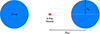 |
Fig. 2. Torus geometry in REFLEX. The inner radius, Rin, is defined as the radius of the cross-section, while the outer radius, Rout, is measured from the centre of the torus to the centre of the cross-section. The equatorial column density, NH,eq, is measured across the diameter of the cross-section (white dashed line). The X-ray point source is placed at the centre of the torus. |
For the two models that include only the torus, we placed the X-ray point source at the centre of the torus as a good approximation. In all cases, we chose a power-law emission spectrum for the X-ray source with typical values for the photon index, Γ = 1.9, and high-energy exponential cut-off, EC = 200 keV (e.g. Ricci et al. 2017a, 2018).
3.3.1. Simple torus
We started from the simple unification of AGNs, which suggests that the observed differences between type-I and type-II AGNs are caused only by orientation effects depending on the observer’s line of sight (Antonucci 1993). Our model is composed of an obscuring torus whose Rin/Rout ratio is a free parameter independent of any other AGN properties and remains the same throughout the population. Hence, in this population the only difference between different AGNs is the torus NH,eq. Because the geometry of this model is only dependent on the ratio Rin/Rout, which sets the covering factor, the simulation can be scale-free. We fixed Rin = 0.5 (in arbitrary units) and let Rout vary as Rout = Rin + R1, with R1 being a free positive parameter.
3.3.2. Luminosity-dependent torus
We chose our next physically motivated model to include a relationship between the location of the inner edge of the torus and the luminosity. Thus, we constructed a model based on the ‘receding torus’ (Lawrence 1991), which is often invoked to explain the decrease of the fraction of absorbed AGNs as a function of luminosity. In fact, it applies to a dusty torus, where the dust is destroyed when it reaches a temperature of ∼1500K (see Nenkova et al. 2008) due to irradiation by the central engine. In the receding-torus model, the inner edge of the obscuring torus, rdust = Rout − Rin, is set by the dust-sublimation radius, which increases with luminosity as rdust ∝L0.5. Therefore, if dust-free gas behaves as dusty gas, the fraction of absorbed AGNs is expected to scale as ∝ L−0.5 at high luminosities.
Our luminosity-dependent (LD) model introduces a dependence of the covering factor of the scaleless tori on the intrinsic X-ray luminosity of the AGNs, with the assumption that gas behaves similarly to dust. We let the slope of the dependence vary because the 0.5 index of the receding torus model does not agree with observations of the absorbed fraction in the X-rays, which find a much flatter slope (e.g. H08, Burlon et al. 2011). We discuss the possible mechanisms for this in Sect. 5.1. For practical reasons, we again fixed Rin = 0.5 (in arbitrary units) and let Rout scale with luminosity as
 (3)
(3)
where L0 = 1044 erg s−1 is arbitrarily fixed, and R0 and α are free parameters.
3.3.3. Accretion disc
To make our model more realistic, we added a flat, optically thick, dust-free annulus to the previous model to simulate the presence of an accretion disc (AD). The outer radius of the annulus is set as Rdisc ≡ rdust = Rout − Rin, so that the torus is its physical continuation (Fig. 3). This model (hereafter LD+AD) cannot be scaleless because the height of the X-ray source is not related to other distances, such as the inner edge of the torus. Instead, we fixed Rin = 1pc (e.g. Ramos Almeida & Ricci 2017) and the inner radius of the annulus to rdisc = 6rg (e.g. Wilkins & Fabian 2011), where rg = 2 G MBH / c2 is the Schwarzschild gravitational radius and assuming a typical SMBH mass of MBH = 107 M
 (e.g. Koss et al. 2017). We set H and He to be fully ionised, although since the disc is completely optically thick, this choice has a negligible effect on the simulated spectra.
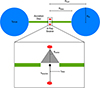 |
Fig. 3. Accretion-disc and double-X-ray-source geometry in REFLEX (not to scale). The outer radius of the thin annulus representing the AD is set as Rdisc = Rout − Rin, with Rin = 1pc, and the inner radius of the annulus as rdisc = 6rg. We place a double X-ray point source above and below the centre of the annulus at hsource = 10rg. The grey area represents the cone defined by hsource and rdisc, inside which we do not allow the sources to emit, as in reality emission through the centre of the annulus would be blocked by the SMBH. The half-opening angle of the cone, θcone = arctan(rdisc / hsource), is denoted by the dashed lines. |
For this model, we placed a double X-ray point source located above and below the centre of the annulus at hsource = 10rg, following the lamppost geometry (Martocchia & Matt 1996; Miniutti & Fabian 2004). For the purposes of this study, we adopted the lamppost geometry as a widely used and longstanding approximation of the X-ray source despite its known limitations (e.g. Tagliacozzo et al. 2023), since the geometry of the compact corona has negligible effects on the properties of the reflected radiation. To prevent the escape of emission through the centre of the annulus, which in reality would be blocked by the SMBH, we forced the emission of the sources to remain outside the cones defined by hsource and rdisc (as shown in Fig.3), and we corrected the intrinsic luminosity of each object in our population by the factor (1 − cos θcone) / 2, where θcone = arctan(rdisc / hsource) is the half-opening angle of the cones.
3.4. Synthetic population
After defining the models, we created a large sample of AGNs for which we simulate the X-ray emission and determined absorption properties. For each object in our synthetic population, we drew the redshift and intrinsic 2–10 keV X-ray luminosity of the X-ray source by sampling the XLF derived in U03, the observation angle, θobs, from a cosine distribution between 0° and 90°, and the equatorial column density, NH,eq, of the torus (Fig. 2) from a log-normal distribution, log(NH,eq/ cm−2)∼𝒩(μ, σ), where μ and σ are the mean and the standard deviation of the distribution, respectively, and free parameters in all our models.
We calculated the line-of-sight column density of the homogeneous torus, NH, at a certain observation angle, θobs, as shown in Paltani & Ricci (2017):
 (4)
(4)
We performed numerical simulations using REFLEX to create a grid of models of AGN X-ray spectra in the 2–100 keV energy range, with log(NH,eq/cm−2) between 21 and 26 with a step of 0.1, and log(Rin/Rout) between −2 and 0 with a step of 0.05. We then interpolated from the grid to obtain the spectrum of any AGN in our population. For practical reasons, the grid was computed at z = 0.0001, and the final spectra were obtained by redshifting the ones interpolated from the grid and rescaling the flux according to the luminosity distance.
To represent the diverse populations from which each observable is derived, we created subsamples of our synthetic population. For the reproduction of the CXB, we drew objects with  erg s−1 and z ≤ 3, as non-blazar AGNs beyond this redshift are expected to contribute only ∼1% (Figs. 14 and 15 in Ueda et al. 2014). For the NH distribution from R17, we sampled up to z = 0.3, since BAT is only sensitive to objects in the local Universe. Drawing objects at random from the XLF would result in large statistical fluctuations at low redshift, where the volume is small, and at high luminosity, where objects are rare. To avoid these stochastic effects and to remove the effect of cosmic variance in the simulations, we divided the redshift ranges considered for each observable into ten redshift bins. We then drew the same large number of objects, Nsample, in each redshift bin. As a different number of objects, NXLF, is expected when integrating the log(NH/cm−2) < 24 XLF, each object is assigned a weight NXLF/(Nsample−NCT), where NCT is the number of CT objects in our population within each redshift bin.
To correct our synthetic sample for the effect of absorption and compare our results to the observational constraints from R17 and H08, we used the sensitivity curves of the Swift/BAT 70-month catalogue (Baumgartner et al. 2013) and of the ten samples combined in H08, respectively. We expressed the sensitivity curves as the sky fraction as a function of 14–195 keV and 2–10 keV flux limit for each study, which we show in Fig. 4. Using REFLEX, we obtained the fluxes of each simulated source in the respective energy bands and applied a weight determined by the probability of such an object being detected according to the sky fraction. This effectively applies the selection functions of these studies to our simulated population.
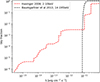 |
Fig. 4. Sky fraction as a function of 14–195 keV and 2–10 keV flux limits representing the sensitivity curves of the Swift/BAT 70-month survey used in R17 (black line) and the multiple surveys used in H08 (red line), respectively. |
4. Results
Following the creation of a synthetic AGN population and the simulation of their X-ray spectra, we determined the parameter posterior distributions of our models based on three data sets: (a) the CXB; (b) the three observed absorption properties –namely the fraction of NH in bins of log(NH) and the fraction of absorbed AGNs as a function of observed 2–10 keV luminosity, and as a function of redshift; and (c) all four constraints combined.
4.1. Simulation-based inference
We determined model parameters using the simulation-based inference (SBI) approach, as implemented in the Python package sbi (Tejero-Cantero et al. 2020). SBI maps the relationship between simulated data and model parameters by constructing their joint density in the data and parameter space using a deep neural network. This approach is completely likelihood-free. We added noise to our practically noiseless simulated data to match the uncertainties in the observed data. For the CXB, we added Gaussian noise in each bin using the variance observed in the data. For the absorption properties, the noise was applied in each bin by drawing from a binomial distribution, with the success probability given by the model and the number of trials given by the number of ’observed’ objects.
We used the sequential neural posterior estimation (SNPE) (Greenberg et al. 2019), which allows us to directly sample the posterior distribution of our parameters given the data. In the SNPE, the density is initially learned across the parameter priors (see Table 1) with a relatively small number of training samples. We then constructed the covariance matrix of the posteriors, which we used to provide a proposal prior in the form of a multivariate normal distribution for a second iteration of SNPE. This process accelerates the convergence of the deep neural-network training. Depending on the number of free parameters in each model (three or four), we trained the neural estimator using 2000 and 5000 simulations, respectively, to construct the proposal prior; then, we retrained with 5000 and 10 000 simulations, respectively, using the proposal prior. We find that these sizes for the training sets provide stable posterior estimates.
While model comparison can be performed in principle with any parameter inference algorithm that generates samples from the posterior (e.g. McEwen et al. 2021), we adopted a simple metric here to compare the performance of the different models: namely the χ2 statistic of the median models drawn from the posteriors. Indeed, we do not expect that the simple models we explore are able to fully represent the data, so that a statistically rigorous model comparison is not warranted.
4.2. CXB
Median values of the parameter posterior distributions and reduced χ2 values for each model applied to the three observational data sets.
We first tested the ability of our models to reproduce the CXB data set. As shown in Fig. 5, the simple torus model is sufficient to match the CXB, proving that the CXB can be reproduced by even the simplest AGN unification models and, consequently, does not possess a strong constraining power. In Table 2, we summarise the median values of the parameter posteriors and the corresponding reduced χ2 values. All posterior distributions are presented in Appendix A. In this AGN population, if observed edge-on, almost 92% of the AGNs would be CT, since the log-normal distribution of NH,eq is centred around log(NH,eq/ cm−2) = 24.4 with a scatter of only a factor of ∼ 1.4.
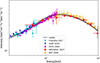 |
Fig. 5. Median model (black line) for CXB in the 2–100 keV range using the simple torus applied only to the CXB data set. The grey region represents the 68% confidence interval of the model based on the posterior distribution of the parameters. |
The LD torus model can reproduce the CXB as well with model parameters close to those of the simple torus model and the posterior distribution of the slope in Eq. (3) showing a median value near 0.
4.3. Absorption properties
We next applied our models to the three absorption data sets. The limitations of the simple torus model become evident when applied to the absorption properties, even when the CXB constraint is ignored. In this case, the model fails to reproduce the observed anti-correlation between the absorbed fraction and luminosity (top row of Fig. 6).
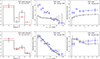 |
Fig. 6. Median models (black lines) for the three observed absorption properties using the simple torus model (top row) and the LD torus (bottom row) applied only to the three absorption data sets. Left: Fraction of NH in bins of log(NH). Middle: Absorbed fraction of AGNs as a function of observed LX(2–10 keV). Right: Absorbed fraction of AGNs as a function of redshift. The error bars on the models represent their 68% confidence interval based on the posterior distribution of the parameters. |
In contrast, the LD torus model reproduces the three constraints very well (bottom row of Fig. 6). In this case, the posterior distribution of the slope in Eq. (3) yields a median value of α = 0.41 , which is close to, but still different from, the predictions of the receding torus model. Furthermore, matching the absorption properties requires the log-normal distribution of NH,eq to be more than three times broader and centred 0.66 dex lower compared to the optimal match on the CXB. This, combined with the strong luminosity dependence of the covering factor, results in a distinctly different AGN population than the one that best reproduces the CXB. Specifically, for the CXB, approximately 55% of the synthetic population needs to be CT and only ∼13% Compton-thin, whereas for the absorption properties, the fractions shift to around 33% CT and 51% Compton-thin.
4.4. Combined constraints
Finally, after demonstrating the distinct differences between the two AGN populations that best match the CXB and the absorption properties separately, we sought one population that satisfies all four constraints simultaneously. Given that the simple torus model clearly fails to reproduce the absorption properties, we did not apply it to the combined data sets, focusing instead on the LD torus model. For simplicity, we calculated the combined χ2 without applying any particular weight to the data sets, despite the heteroscedasticity of the combined set. In Fig. 7, we show the CXB and the absorption properties reproduced by the LD torus. While most constraints are adequately matched, the model completely fails to explain the shape of the NH fraction in bins of log(NH), underestimating the number of less obscured objects and overestimating that of heavily obscured objects. The failure of the LD model to reproduce our combined constraints highlights the need for a more complex model to better capture the observed properties of the AGN population.
 |
Fig. 7. Median models (black lines) using the LD torus model applied to the combined constraints. From the left: CXB, the observed fraction of NH in bins of log(NH), the absorbed fraction of AGNs as a function of observed LX(2–10 keV), and the absorbed fraction of AGNs as a function of redshift. The grey region and error bars represent the 68% confidence interval of the model based on the posterior distribution of the parameters. |
Building on the limitations of the LD torus model, we now turn to the LD+AD model to assess whether it can provide a better match to the combined observational constraints. While this model provides the best simultaneous match to all four constraints (shown in Fig. 8), it significantly underpredicts the CXB at high energies and predicts an ∼25% lower absorbed AGN fraction at high redshifts. The posterior distribution of the slope in Eq. (3) yields a median value of α = 0.24 , substantially deviating from the predictions of the receding torus model, but in close agreement with X-ray observations (e.g. Burlon et al. 2011; Sazonov et al. 2015). The log-normal distribution of NH,eq of this population aligns very closely with that of the best match on the absorption properties –rather than the CXB– further demonstrating that the CXB does not carry enough constraining power. Even then, the posterior distributions of the normalisation, R0, and the slope, α, in Eq. (3) have medians that are more than twice as high and nearly twice as flat, respectively, compared to the best match to the absorption properties. The combined constraints result in the lowest fraction of CT AGNs (∼21%) and a Compton-thin fraction of ∼48%, leaving an unobscured fraction of ∼31%.
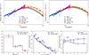 |
Fig. 8. Same as Fig. 7, but using the LD+AD model. Top left: CXB with fixed high-energy cut-off EC = 200 keV; top right: that with EC = 300 keV (see Sect. 4.4 for more information). |
To address the underpredicted CXB at high energies, we increased the fixed high-energy cut-off of the X-ray source from EC = 200 keV to EC = 300 keV, as low-accretion AGNs are more common and tend to have higher EC (R17; Ricci et al. 2018; Baloković et al. 2020). Since variations in EC affect the high-energy region of the AGN spectra while having minimal impact on the lower energy range, we find that redetermining model parameters does not result in significant changes to the parameter posteriors. Using the same parameter posteriors, we find that the match to the CXB improves considerably (top right in Fig. 8), while the absorption properties remain consistent.
5. Discussion
Our results demonstrate that the CXB can be reproduced not only by more complex models, but even by the simple unification model of AGNs. However, our simple torus model lacks some necessary ingredients to accurately represent the absorption properties. First, the covering factor of the absorber must have a clear luminosity dependence, which cannot be constrained by the CXB alone. Second, the inclusion of the AD component is essential to provide enough reflection given the constraint of the NH distribution. Hence, the LD+AD model is the only realistic model capable of simultaneously matching both the CXB and the absorption data sets. Nevertheless, all models discussed in this work are simplistic and cannot be expected to explain the full phenomenology of AGNs in detail.
5.1. Luminosity dependence of absorbed fraction
As shown in Sect. 4.4, when applying the LD+AD model to all observational constraints simultaneously, we were able to reproduce the dependence of the absorbed fraction on the X-ray luminosity. From parameter determination, we can derive that the inner edge of typical dusty tori, rdust = Rout − Rin, spans a range of 0.2–2.8 pc in the L range 1041 − 1046 erg s−1, which is consistent with dust sublimation radius sizes found in infrared interferometry studies (e.g. Tristram et al. 2014; GRAVITY Collaboration 2020). However, we find a shallow median slope in Eq. (3), α = 0.24
 , which is compatible with observational studies in the X-rays (e.g. Burlon et al. 2011; Sazonov et al. 2015), but in disagreement with the receding torus model. As a further investigation, Fig. 9 shows the average covering factor of the detected tori in our local AGN population as a function of intrinsic 14–150 keV luminosity to compare with the Swift/BAT results from Ricci et al. (2022). We find that the covering factor decreases by 27% across the LX(14 − 150 keV) range of 1042 − 1045 erg s−1, in very good agreement with Ricci et al. (2022) despite our model being constrained by the absorbed fraction from H08 that comprises a population up to z = 3.2 detected in the 2–10 keV.
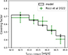 |
Fig. 9. Average torus covering factor of our local synthetic population as a function of intrinsic 14–150 keV luminosity using the LD+AD model (black). The error bars represent the 68% confidence interval of the model based on the posterior distribution of the parameters. For comparison, the covering factor of Swift/BAT-detected AGNs from Ricci et al. (2022; green). |
Other mechanisms have been proposed to explain the luminosity dependence of the absorbed fraction with a slope flatter than that predicted by the receding torus model. Additional X-ray obscuration could arise from the broad-line region (BLR), which is located within the dust sublimation radius. The presence of absorption in the BLR could increase the fraction of absorbed AGNs at high luminosity, thus flattening the relationship between the absorbed fraction and luminosity. Another important mechanism is the clumpy dusty-torus model (e.g. Nenkova et al. 2008), from which Hönig & Beckert (2007) predicted that the absorbed fraction decreases as ∝L−0.25 due to the interplay between radiation pressure and the clump distribution. It must be pointed out that the recent studies of Ricci et al. (2017b, 2022) have revealed that when the AGNs are binned by Eddington ratio, the luminosity dependence of the absorbed fraction completely flattens. Instead, they propose a radiation-regulated unification model, where the absorbed fraction depends on the Eddington ratio rather than luminosity.
As a direct consequence of the relation between absorption and luminosity, our LD+AD model predicts that absorbed and unabsorbed AGNs have different XLFs. In Fig. 10, we present the two XLFs of our population up to z = 0.1. Our model predicts well the increase of absorbed AGNs below log(LX) = 43.5, as found by the model of Aird et al. (2015) extrapolated to z = 0 (taken from their Fig. 13) and the local observations in Burlon et al. (2011; converted to 2–10 keV luminosities). Our model confirms that absorbed AGNs are intrinsically less luminous. Both our absorbed and unabsorbed XLFs agree very well with the results of Burlon et al. (2011), but our unabsorbed XLF deviates from the results of Aird et al. (2015) at low luminosities. That may be because the latter is mostly constrained by high-redshift sources.
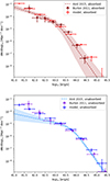 |
Fig. 10. X-ray luminosity function of absorbed (red points) and unabsorbed (blue points) AGNs in our population up to z = 0.1, using the LD+AD model with our combined constraints. The error bars represent the 68% confidence interval of the model based on the posterior distribution of the parameters. Top: Comparison of absorbed XLF with Fig. 13 of Aird et al. (2015), where they extrapolated their model at z = 0 (brown dashed line) and present the local observations of Burlon et al. (2011) converted to 2–10 keV luminosities (brown triangles). Bottom: Same comparison of unabsorbed XLF with Aird et al. (2015) (blue dashed line) and Burlon et al. (2011) (purple triangles). |
5.2. AGN number counts
In Fig. 11, we present AGN differential number counts as a function of flux in the 2–10 keV, 8–24 keV, and 14–195 keV energy bands as reproduced by the LD+AD model. The model predicts the 2–10 keV number counts from the 4 Ms CDFS (Lehmer et al. 2012), XMM-CDFS (Ranalli et al. 2013), and 2XMM (Mateos et al. 2008) surveys well, particularly at fainter fluxes. Similarly, in the 8–24keV band, the model can reproduce the number counts from the combined surveys of NuSTAR (Harrison et al. 2016).
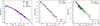 |
Fig. 11. Differential number counts as a function of flux produced by the LD+AD model (black) in the left: 2–10 keV energy range; centre: 8–24 keV range; and right: 14–195 keV range. The error bars represent the 68% confidence interval of the model based on the posterior of the parameters. For comparison, we present the differential number counts of the 70-month Swift/BAT (Ananna et al. 2022, green), combined NuSTAR (Harrison et al. 2016, brown), 4 Ms CDFS (Lehmer et al. 2012, red), XMM-CDFS (Ranalli et al. 2013, blue), and 2XMM (Mateos et al. 2008, magenta) surveys. |
By contrast, the model consistently overpredicts the 14–195 keV Swift/BAT differential number counts (Ananna et al. 2022) within 1σ–2σ. We note that this is in agreement with several other AGN population-synthesis models based on the CXB (e.g. Gilli et al. 2007; Ueda et al. 2014; Aird et al. 2015), which also produce higher number counts than Swift/BAT, as shown in Ananna et al. (2019) and Harrison et al. (2016). This tension is still under investigation (e.g. Akylas & Georgantopoulos 2019; Delaney et al. 2023).
5.3. Reflection versus obscuration
In Fig. 12, we compare the predicted reflection of our models to the observed trend between reflection and line-of-sight NH reported in Panagiotou et al. (2021), Ricci et al. (2011), and Esposito & Walter (2016). We computed the fraction of reflected-to-total emission (Fref / Ftotal) in the 14–195 keV band using REFLEX for our LD and LD+AD models. Although these previous studies suggest an increase of reflection with obscuration, large uncertainties and unknown selection effects make this correlation debatable and not statistically conclusive. We therefore used the data for qualitative comparison only, by replacing the reflection parameter of the pexrav model in XSPEC (Arnaud 1996) with Fref / Ftotal in the same energy band.
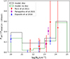 |
Fig. 12. Observed correlation between the fraction of reflected emission over total emission, Fref / Ftotal, in the 14–195 keV energy band and the line-of-sight NH; these were produced with our combined constraints’ median parameters for the LD+AD model (black line) and the LD torus model (green line). The data are from Panagiotou et al. (2021), Esposito & Walter (2016), and Ricci et al. (2011) (magenta, blue, and red points, respectively) after replacing the reflection parameter of the pexrav model in XSPEC with the fraction Fref / Ftotal in the same energy band. |
Both models broadly follow the trend of increasing reflection with obscuration, while they also predict the increase of reflection for unobscured sources [log(NH/ cm−2) < 21], which was suggested in Esposito & Walter (2016) and Panagiotou & Walter (2019). The key difference between our models arises at log(NH/ cm−2) < 23, where the LD+AD model consistently provides optically thick material necessary to produce reflection. In comparison, the LD model lacks such material in this NH range, resulting in nearly half the reflection predicted by the LD+AD model.
While Ricci et al. (2011) and Panagiotou et al. (2021) attributed enhanced reflection in heavily obscured sources to a clumpy dusty torus, we demonstrate that such a trend can also emerge from our homogeneous torus models. Nonetheless, a clumpy torus could alter this relationship by introducing variability in the line of sight, as it allows the encountering of different NH for the same orientation at different azimuthal angles. This may contribute to the observed scatter and could be explored in future work.
5.4. Intrinsic fraction of Compton-thick AGNs
We derived the intrinsic CT fraction (log(NH/cm−2)≥24) with the LD and LD+AD models and find that it drops from 50 ± 2% (68% confidence based on the posteriors) without the AD to 21 ± 7% with the AD. As shown in Fig. 12, when adding the AD, the unobscured and Compton-thin AGNs produce more reflection without additional absorption, reducing the amount of CT AGNs needed to reproduce the CXB peak. As the LD+AD model is more realistic and best reproduces all constraints, the CT fraction of 21 ± 7% is likely closer to the true value. This aligns very well with the findings of local X-ray surveys (e.g. Burlon et al. 2011; Ricci et al. 2015; Boorman et al. 2025) and with the predictions of previous AGN population syntheses at low redshift (e.g. Ueda et al. 2014; Aird et al. 2015). However, at z = 1, Ueda et al. (2014) and Ananna et al. (2019) predicted an intrinsic CT fraction of 37 ± 2% and 56 ± 7%, respectively. The discrepancy with our value likely arises at least in part because our model does not take into account redshift evolution, causing the CT fraction of the parent population to remain constant. This limitation may also explain why our model struggles to accurately match the absorbed AGN fraction at higher redshifts (however, see Sect. 5.5 for an alternative explanation). To incorporate evolution in our model, an additional parameter would be needed to evolve the size or density of the dusty torus, which is beyond the scope of this work.
In Fig. 13, we further compare the contribution of unobscured [log(NH/cm−2) < 22], Compton-thin [22 ≤ log(NH/cm−2) < 24], and CT sources [log(NH/cm−2)≥24] to the CXB with the LD and LD+AD models. The total contribution of CT objects to the CXB in the 14–195 keV range is found to be ∼28% for the LD model, while the CT contribution drops to about 7% with the LD+AD model. The latter value is in close agreement with that found by Treister et al. (2009).
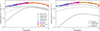 |
Fig. 13. Left: Contribution of unobscured (log(NH/ cm−2 < 22; dashed-dotted line), Compton-thin (22 ≤ log(NH/cm−2) < 24; dotted line), and CT sources (log(NH/cm−2)≥24; dashed line) to the CXB (solid line) reproduced by the median parameters of the LD torus model. Right: As before, but for the LD+AD model. |
Finally, in Fig. 14, we present the intrinsic line-of-sight NH distribution of our local population of AGNs using the LD+AD model. The distribution reveals the same bimodality seen in the observed one, with peaks in the log(NH/cm−2) = 20–21 and 23–24 bins. Our model recovers the results from Ricci et al. (2015) well, although they assumed a fixed covering factor when correcting the observed NH distribution into the intrinsic one. For reference, we also included the observed distribution of our model from Fig. 8, with the first two bins separated. The selection bias is most significant for completely unobscured and CT AGNs, as expected.
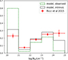 |
Fig. 14. Intrinsic NH distribution (black line) of our local synthetic population produced using the LD+AD model with the combined constraints. Our observed distribution (green line) from Fig. 8 and the intrinsic distribution from Ricci et al. (2015) (red points) are shown for comparison. |
5.5. Origin of mildly obscured AGNs
As discussed in Sect. 2.2, our models do not contain the ingredients to generate a population with a significant fraction of mildly obscured AGNs [log(NH/cm−2) < 22]. One possible origin of obscuration in these AGNs is the gas and dust in the plane of the host galaxy around our dusty torus, which would cause completely unobscured objects to be subject to additional absorption of log(NH/cm−2) < 22. Gilli et al. (2022) constructed a clumpy interstellar medium (ISM) whose characteristic cloud surface density evolves with redshift and used it in combination with the obscuring torus to reproduce the fraction of absorbed AGNs as a function of redshift from deep X-ray studies (e.g. Buchner et al. 2015; Iwasawa et al. 2020). They find that the median NH of the ISM evolves as ∝(1 + z)3.3, assuming a median NH = 1021 cm−2 for local galaxies (Willingale et al. 2013).
Hence, if we incorporate this component into our model, the ISM NH could increase by up to ∼2.4 times within our local (z < 0.3) synthetic population, which is used to reproduce the observed fraction of NH in bins of log(NH). This increase would be sufficient to shift a significant fraction of completely unobscured objects into the log(NH/cm−2) = 21–22 bin. Furthermore, in the redshift range z = 1.2 − 3.2, the ISM NH would increase from ∼13 times to more than 100 times. This could result in the increase of the absorbed fraction at higher redshift, which our current model underpredicts. Regarding our model parameters, incorporating the ISM would likely cause the posterior of the mean, μ, of the NH,eq distribution to shift to lower values. Our results on the CXB would likely not be significantly affected, since the biggest difference would be high redshift sources that are obscured (see right of Fig. 13).
6. Conclusions
Until now, population-synthesis AGN models have not treated absorption and reflection self-consistently, but rather assumed values for the reflection at different obscurations and for the intrinsic fraction of CT AGNs. We created a fully self-consistent population-synthesis AGN model with numerical simulations of their X-ray emission using the ray-tracing code REFLEX. Our constraints include the CXB as well as absorption properties of AGNs detected in different X-ray surveys, namely the fraction of NH in bins of log(NH) and the fraction of absorbed AGNs as a function of observed LX and as a function of redshift. We sampled an intrinsic XLF and parameterised the geometry and density of the circumnuclear material of the AGN population. We constructed geometrical models based on the simple unification of AGNs and the receding torus; lastly, we included an AD. We determined the parameter posterior distributions for each model using an SBI method.
We find that the CXB can be well reproduced, even by the simple torus model (Fig. 5). However, matching the absorption properties requires the LD torus model (Fig. 6). The LD+AD model best satisfies all observational constraints simultaneously (Fig. 8). In this case, the posterior distribution of the slope in Eq. (3) has a median of α = 0.24 , in agreement with X-ray observations.
We derive an intrinsic CT fraction of 21 ± 7% (68% confidence based on the posteriors), in agreement with observations of the local Universe, and find that the inner edge of the dusty torus spans a range of 0.2–2.8 pc in the L range 1041 − 1046 erg s−1; this is consistent with dust sublimation radius sizes from infrared interferometry studies. Our synthetic population can reproduce the luminosity dependence of the torus covering factor and XMM-Newton, Chandra, and NuSTAR number counts, as well as the observed correlation between reflection and obscuration (Figs. 9, 11, and 12). Additionally, it can recover the XLFs of absorbed and unabsorbed AGNs and the intrinsic NH distribution of local AGNs. However, our AGN modelling lacks the obscuration originating at the host galaxy as well as evolution, resulting in a lower fraction of absorbed AGNs at high redshifts and a constant CT fraction.
This is the first work in which the CXB is reproduced with a fully self-consistent synthetic AGN-population model, without assuming the reflection features of the spectra, the intrinsic NH distribution, or the CT fraction, and without modifying the XLF. Modelling and linking the emission, absorption, and reflection through the matter distribution allowed us to break the degeneracy of fitting the CXB by simultaneously matching observational constraints concerning absorption, which has not been done before. Overall, our results emphasise that a better understanding of AGNs requires models that account for both the geometric structure and the physical mechanisms of the absorbers in order to explain their observed properties. In the future, this methodology can be extended to include more complex models that can account for effects such as the clumpiness of the obscuring material, evolution, or additional relationships between AGN parameters, introducing in particular the intrinsic properties of SMBHs, such as their mass and Eddington ratio.
Acknowledgments
CR acknowledges support from Fondecyt Regular grant 1230345, ANID BASAL project FB210003 and the China-Chile joint research fund.
References
- Aird, J., Coil, A. L., Georgakakis, A., et al. 2015, MNRAS, 451, 1892 [Google Scholar]
- Ajello, M., Greiner, J., Sato, G., et al. 2008, ApJ, 689, 666 [Google Scholar]
- Akylas, A., & Georgantopoulos, I. 2019, A&A, 625, A131 [NASA ADS] [CrossRef] [EDP Sciences] [Google Scholar]
- Akylas, A., Georgakakis, A., Georgantopoulos, I., Brightman, M., & Nandra, K. 2012, A&A, 546, A98 [NASA ADS] [CrossRef] [EDP Sciences] [Google Scholar]
- Ananna, T. T., Treister, E., Urry, C. M., et al. 2019, ApJ, 871, 240 [Google Scholar]
- Ananna, T. T., Weigel, A. K., Trakhtenbrot, B., et al. 2022, ApJS, 261, 9 [NASA ADS] [CrossRef] [Google Scholar]
- Antonucci, R. 1993, ARA&A, 31, 473 [Google Scholar]
- Arnaud, K. A. 1996, ASP Conf. Ser., 101, 17 [Google Scholar]
- Baloković, M., Harrison, F. A., Madejski, G., et al. 2020, ApJ, 905, 41 [Google Scholar]
- Baumgartner, W. H., Tueller, J., Markwardt, C. B., et al. 2013, ApJS, 207, 19 [Google Scholar]
- Boorman, P. G., Gandhi, P., Buchner, J., et al. 2025, ApJ, 978, 118 [Google Scholar]
- Brandt, W. N., & Alexander, D. M. 2015, A&ARv, 23, 1 [Google Scholar]
- Brandt, W. N., & Yang, G. 2022, in Handbook of X-ray and Gamma-ray Astrophysics, eds C. Bambi, & A. Sangangelo, 78 [Google Scholar]
- Brightman, M., & Nandra, K. 2011, MNRAS, 413, 1206 [NASA ADS] [CrossRef] [Google Scholar]
- Buchner, J., Georgakakis, A., Nandra, K., et al. 2015, ApJ, 802, 89 [Google Scholar]
- Burlon, D., Ajello, M., Greiner, J., et al. 2011, ApJ, 728, 58 [Google Scholar]
- Cappelluti, N., Ranalli, P., Roncarelli, M., et al. 2012, MNRAS, 427, 651 [Google Scholar]
- Cappelluti, N., Li, Y., Ricarte, A., et al. 2017, ApJ, 837, 19 [NASA ADS] [CrossRef] [Google Scholar]
- Churazov, E., Sunyaev, R., Revnivtsev, M., et al. 2007, A&A, 467, 529 [NASA ADS] [CrossRef] [EDP Sciences] [Google Scholar]
- Delaney, J. N., Aird, J., Evans, P. A., et al. 2023, MNRAS, 521, 1620 [CrossRef] [Google Scholar]
- Draine, B. T. 2003, ApJ, 598, 1026 [Google Scholar]
- Draper, A. R., & Ballantyne, D. R. 2009, ApJ, 707, 778 [Google Scholar]
- Esposito, V., & Walter, R. 2016, A&A, 590, A49 [NASA ADS] [CrossRef] [EDP Sciences] [Google Scholar]
- Gebhardt, K., Bender, R., Bower, G., et al. 2000, ApJ, 539, L13 [Google Scholar]
- Ghisellini, G., Haardt, F., & Matt, G. 1994, MNRAS, 267, 743 [Google Scholar]
- Gilli, R., Comastri, A., & Hasinger, G. 2007, A&A, 463, 79 [NASA ADS] [CrossRef] [EDP Sciences] [Google Scholar]
- Gilli, R., Norman, C., Calura, F., et al. 2022, A&A, 666, A17 [NASA ADS] [CrossRef] [EDP Sciences] [Google Scholar]
- GRAVITY Collaboration (Dexter, J., et al.) 2020, A&A, 635, A92 [NASA ADS] [CrossRef] [EDP Sciences] [Google Scholar]
- Greenberg, D. S., Nonnenmacher, M., & Macke, J. H. 2019, ArXiv e-prints [arXiv:1905.07488] [Google Scholar]
- Gruber, D. E., Matteson, J. L., Peterson, L. E., & Jung, G. V. 1999, ApJ, 520, 124 [NASA ADS] [CrossRef] [Google Scholar]
- Güver, T., & Özel, F. 2009, MNRAS, 400, 2050 [Google Scholar]
- Haardt, F., & Maraschi, L. 1991, ApJ, 380, L51 [Google Scholar]
- Harrison, F. A., Aird, J., Civano, F., et al. 2016, ApJ, 831, 185 [NASA ADS] [CrossRef] [Google Scholar]
- Hasinger, G. 2008, A&A, 490, 905 [NASA ADS] [CrossRef] [EDP Sciences] [Google Scholar]
- Hickox, R. C., & Alexander, D. M. 2018, ARA&A, 56, 625 [Google Scholar]
- Hönig, S. F., & Beckert, T. 2007, MNRAS, 380, 1172 [CrossRef] [Google Scholar]
- Iwasawa, K., Comastri, A., Vignali, C., et al. 2020, A&A, 639, A51 [NASA ADS] [CrossRef] [EDP Sciences] [Google Scholar]
- Kormendy, J., & Ho, L. C. 2013, ARA&A, 51, 511 [Google Scholar]
- Koss, M., Trakhtenbrot, B., Ricci, C., et al. 2017, ApJ, 850, 74 [Google Scholar]
- Lawrence, A. 1991, MNRAS, 252, 586 [NASA ADS] [Google Scholar]
- Lehmer, B. D., Xue, Y. Q., Brandt, W. N., et al. 2012, ApJ, 752, 46 [NASA ADS] [CrossRef] [Google Scholar]
- Liu, T., Tozzi, P., Wang, J.-X., et al. 2017, ApJS, 232, 8 [NASA ADS] [CrossRef] [Google Scholar]
- Lodders, K. 2003, ApJ, 591, 1220 [Google Scholar]
- Magorrian, J., Tremaine, S., Richstone, D., et al. 1998, AJ, 115, 2285 [Google Scholar]
- Martocchia, A., & Matt, G. 1996, MNRAS, 282, L53 [NASA ADS] [CrossRef] [Google Scholar]
- Mateos, S., Warwick, R. S., Carrera, F. J., et al. 2008, A&A, 492, 51 [NASA ADS] [CrossRef] [EDP Sciences] [Google Scholar]
- McEwen, J. D., Wallis, C. G. R., Price, M. A., & Spurio Mancini, A. 2021, ArXiv e-prints [arXiv:2111.12720] [Google Scholar]
- McKaig, J., Ricci, C., Paltani, S., & Satyapal, S. 2022, MNRAS, 512, 2961 [NASA ADS] [CrossRef] [Google Scholar]
- Miniutti, G., & Fabian, A. C. 2004, MNRAS, 349, 1435 [NASA ADS] [CrossRef] [Google Scholar]
- Moretti, A., Pagani, C., Cusumano, G., et al. 2009, A&A, 493, 501 [NASA ADS] [CrossRef] [EDP Sciences] [Google Scholar]
- Nenkova, M., Sirocky, M. M., Nikutta, R., Ivezić, Ž., & Elitzur, M. 2008, ApJ, 685, 160 [Google Scholar]
- Paltani, S., & Ricci, C. 2017, A&A, 607, A31 [NASA ADS] [CrossRef] [EDP Sciences] [Google Scholar]
- Paltani, S., Walter, R., McHardy, I. M., et al. 2008, A&A, 485, 707 [NASA ADS] [CrossRef] [EDP Sciences] [Google Scholar]
- Panagiotou, C., & Walter, R. 2019, A&A, 626, A40 [NASA ADS] [CrossRef] [EDP Sciences] [Google Scholar]
- Panagiotou, C., Walter, R., & Paltani, S. 2021, A&A, 653, A162 [NASA ADS] [CrossRef] [EDP Sciences] [Google Scholar]
- Pounds, K. A., Nandra, K., Stewart, G. C., George, I. M., & Fabian, A. C. 1990, Nature, 344, 132 [NASA ADS] [CrossRef] [Google Scholar]
- Ramos Almeida, C., & Ricci, C. 2017, Nat. Astron., 1, 679 [Google Scholar]
- Ranalli, P., Comastri, A., Vignali, C., et al. 2013, A&A, 555, A42 [NASA ADS] [CrossRef] [EDP Sciences] [Google Scholar]
- Revnivtsev, M., Gilfanov, M., Sunyaev, R., Jahoda, K., & Markwardt, C. 2003, A&A, 411, 329 [NASA ADS] [CrossRef] [EDP Sciences] [Google Scholar]
- Ricci, C., & Paltani, S. 2023, ApJ, 945, 55 [NASA ADS] [CrossRef] [Google Scholar]
- Ricci, C., Walter, R., Courvoisier, T. J. L., & Paltani, S. 2011, A&A, 532, A102 [NASA ADS] [CrossRef] [EDP Sciences] [Google Scholar]
- Ricci, C., Ueda, Y., Koss, M. J., et al. 2015, ApJ, 815, L13 [Google Scholar]
- Ricci, C., Trakhtenbrot, B., Koss, M. J., et al. 2017a, ApJS, 233, 17 [Google Scholar]
- Ricci, C., Trakhtenbrot, B., Koss, M. J., et al. 2017b, Nature, 549, 488 [NASA ADS] [CrossRef] [Google Scholar]
- Ricci, C., Ho, L. C., Fabian, A. C., et al. 2018, MNRAS, 480, 1819 [NASA ADS] [CrossRef] [Google Scholar]
- Ricci, C., Ananna, T. T., Temple, M. J., et al. 2022, ApJ, 938, 67 [NASA ADS] [CrossRef] [Google Scholar]
- Sazonov, S., Churazov, E., & Krivonos, R. 2015, MNRAS, 454, 1202 [NASA ADS] [CrossRef] [Google Scholar]
- Tagliacozzo, D., Marinucci, A., Ursini, F., et al. 2023, MNRAS, 525, 4735 [CrossRef] [Google Scholar]
- Tejero-Cantero, A., Boelts, J., Deistler, M., et al. 2020, J. Open Source Soft., 5, 2505 [Google Scholar]
- Treister, E., Urry, C. M., & Virani, S. 2009, ApJ, 696, 110 [NASA ADS] [CrossRef] [Google Scholar]
- Tristram, K. R. W., Burtscher, L., Jaffe, W., et al. 2014, A&A, 563, A82 [CrossRef] [EDP Sciences] [Google Scholar]
- Ueda, Y., Akiyama, M., Ohta, K., & Miyaji, T. 2003, ApJ, 598, 886 [NASA ADS] [CrossRef] [Google Scholar]
- Ueda, Y., Akiyama, M., Hasinger, G., Miyaji, T., & Watson, M. G. 2014, ApJ, 786, 104 [Google Scholar]
- Wada, K., Papadopoulos, P. P., & Spaans, M. 2009, ApJ, 702, 63 [NASA ADS] [CrossRef] [Google Scholar]
- Wilkins, D. R., & Fabian, A. C. 2011, MNRAS, 414, 1269 [CrossRef] [Google Scholar]
- Willingale, R., Starling, R. L. C., Beardmore, A. P., Tanvir, N. R., & O’Brien, P. T. 2013, MNRAS, 431, 394 [Google Scholar]
- Zappacosta, L., Comastri, A., Civano, F., et al. 2018, ApJ, 854, 33 [Google Scholar]
Appendix
SBI posteriors
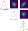 |
Fig. A.1. Parameter posteriors using the simple torus model when applied on the CXB data sets. The median of each distribution reported in Table 2 is denoted in red. |
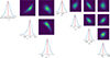 |
Fig. A.2. Parameter posteriors using left: the simple torus model and right: the LD torus model, when applied on the absorption properties. The median of each distribution reported in Table 2 is denoted in red. |
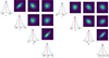 |
Fig. A.3. Parameter posteriors using left: the LD torus model and right: the LD+AD model, when applied on all constraints. The median of each distribution reported in Table 2 is denoted in red. |
All Tables
Median values of the parameter posterior distributions and reduced χ2 values for each model applied to the three observational data sets.
All Figures
|
Fig. 1. X-ray observables used as constraints in this work. From the left: CXB measured by Chandra (cyan; Cappelluti et al. 2017), INTEGRAL (red; Churazov et al. 2007), RXTE (magenta; Revnivtsev et al. 2003), Swift/BAT (orange; Ajello et al. 2008), and Swift/XRT (blue; Moretti et al. 2009). The observed NH distribution of 731 AGNs in the 70-month Swift/BAT catalogue, detected in the 14–195 keV range, from Ricci et al. (2017a). The point with the dashed error bars represents the sum of the first two bins used in this work (see Sect. 2.2 for more information). The absorbed fraction of 1290 AGNs from multiple surveys in the 2–10 keV range is shown as a function of observed luminosity and as a function of redshift from Hasinger (2008). |
| In the text | |
|
Fig. 2. Torus geometry in REFLEX. The inner radius, Rin, is defined as the radius of the cross-section, while the outer radius, Rout, is measured from the centre of the torus to the centre of the cross-section. The equatorial column density, NH,eq, is measured across the diameter of the cross-section (white dashed line). The X-ray point source is placed at the centre of the torus. |
| In the text | |
|
Fig. 3. Accretion-disc and double-X-ray-source geometry in REFLEX (not to scale). The outer radius of the thin annulus representing the AD is set as Rdisc = Rout − Rin, with Rin = 1pc, and the inner radius of the annulus as rdisc = 6rg. We place a double X-ray point source above and below the centre of the annulus at hsource = 10rg. The grey area represents the cone defined by hsource and rdisc, inside which we do not allow the sources to emit, as in reality emission through the centre of the annulus would be blocked by the SMBH. The half-opening angle of the cone, θcone = arctan(rdisc / hsource), is denoted by the dashed lines. |
| In the text | |
|
Fig. 4. Sky fraction as a function of 14–195 keV and 2–10 keV flux limits representing the sensitivity curves of the Swift/BAT 70-month survey used in R17 (black line) and the multiple surveys used in H08 (red line), respectively. |
| In the text | |
|
Fig. 5. Median model (black line) for CXB in the 2–100 keV range using the simple torus applied only to the CXB data set. The grey region represents the 68% confidence interval of the model based on the posterior distribution of the parameters. |
| In the text | |
|
Fig. 6. Median models (black lines) for the three observed absorption properties using the simple torus model (top row) and the LD torus (bottom row) applied only to the three absorption data sets. Left: Fraction of NH in bins of log(NH). Middle: Absorbed fraction of AGNs as a function of observed LX(2–10 keV). Right: Absorbed fraction of AGNs as a function of redshift. The error bars on the models represent their 68% confidence interval based on the posterior distribution of the parameters. |
| In the text | |
|
Fig. 7. Median models (black lines) using the LD torus model applied to the combined constraints. From the left: CXB, the observed fraction of NH in bins of log(NH), the absorbed fraction of AGNs as a function of observed LX(2–10 keV), and the absorbed fraction of AGNs as a function of redshift. The grey region and error bars represent the 68% confidence interval of the model based on the posterior distribution of the parameters. |
| In the text | |
|
Fig. 8. Same as Fig. 7, but using the LD+AD model. Top left: CXB with fixed high-energy cut-off EC = 200 keV; top right: that with EC = 300 keV (see Sect. 4.4 for more information). |
| In the text | |
|
Fig. 9. Average torus covering factor of our local synthetic population as a function of intrinsic 14–150 keV luminosity using the LD+AD model (black). The error bars represent the 68% confidence interval of the model based on the posterior distribution of the parameters. For comparison, the covering factor of Swift/BAT-detected AGNs from Ricci et al. (2022; green). |
| In the text | |
|
Fig. 10. X-ray luminosity function of absorbed (red points) and unabsorbed (blue points) AGNs in our population up to z = 0.1, using the LD+AD model with our combined constraints. The error bars represent the 68% confidence interval of the model based on the posterior distribution of the parameters. Top: Comparison of absorbed XLF with Fig. 13 of Aird et al. (2015), where they extrapolated their model at z = 0 (brown dashed line) and present the local observations of Burlon et al. (2011) converted to 2–10 keV luminosities (brown triangles). Bottom: Same comparison of unabsorbed XLF with Aird et al. (2015) (blue dashed line) and Burlon et al. (2011) (purple triangles). |
| In the text | |
|
Fig. 11. Differential number counts as a function of flux produced by the LD+AD model (black) in the left: 2–10 keV energy range; centre: 8–24 keV range; and right: 14–195 keV range. The error bars represent the 68% confidence interval of the model based on the posterior of the parameters. For comparison, we present the differential number counts of the 70-month Swift/BAT (Ananna et al. 2022, green), combined NuSTAR (Harrison et al. 2016, brown), 4 Ms CDFS (Lehmer et al. 2012, red), XMM-CDFS (Ranalli et al. 2013, blue), and 2XMM (Mateos et al. 2008, magenta) surveys. |
| In the text | |
|
Fig. 12. Observed correlation between the fraction of reflected emission over total emission, Fref / Ftotal, in the 14–195 keV energy band and the line-of-sight NH; these were produced with our combined constraints’ median parameters for the LD+AD model (black line) and the LD torus model (green line). The data are from Panagiotou et al. (2021), Esposito & Walter (2016), and Ricci et al. (2011) (magenta, blue, and red points, respectively) after replacing the reflection parameter of the pexrav model in XSPEC with the fraction Fref / Ftotal in the same energy band. |
| In the text | |
|
Fig. 13. Left: Contribution of unobscured (log(NH/ cm−2 < 22; dashed-dotted line), Compton-thin (22 ≤ log(NH/cm−2) < 24; dotted line), and CT sources (log(NH/cm−2)≥24; dashed line) to the CXB (solid line) reproduced by the median parameters of the LD torus model. Right: As before, but for the LD+AD model. |
| In the text | |
|
Fig. 14. Intrinsic NH distribution (black line) of our local synthetic population produced using the LD+AD model with the combined constraints. Our observed distribution (green line) from Fig. 8 and the intrinsic distribution from Ricci et al. (2015) (red points) are shown for comparison. |
| In the text | |
|
Fig. A.1. Parameter posteriors using the simple torus model when applied on the CXB data sets. The median of each distribution reported in Table 2 is denoted in red. |
| In the text | |
|
Fig. A.2. Parameter posteriors using left: the simple torus model and right: the LD torus model, when applied on the absorption properties. The median of each distribution reported in Table 2 is denoted in red. |
| In the text | |
|
Fig. A.3. Parameter posteriors using left: the LD torus model and right: the LD+AD model, when applied on all constraints. The median of each distribution reported in Table 2 is denoted in red. |
| In the text | |
Current usage metrics show cumulative count of Article Views (full-text article views including HTML views, PDF and ePub downloads, according to the available data) and Abstracts Views on Vision4Press platform.
Data correspond to usage on the plateform after 2015. The current usage metrics is available 48-96 hours after online publication and is updated daily on week days.
Initial download of the metrics may take a while.