| Issue |
A&A
Volume 700, August 2025
|
|
|---|---|---|
| Article Number | A78 | |
| Number of page(s) | 18 | |
| Section | Cosmology (including clusters of galaxies) | |
| DOI | https://doi.org/10.1051/0004-6361/202553927 | |
| Published online | 08 August 2025 | |
Euclid preparation
LXXII. Three-dimensional galaxy clustering in configuration space: Two-point correlation function estimation
1
Aix-Marseille Université, CNRS, CNES, LAM, Marseille, France
2
Dipartimento di Fisica e Astronomia “Augusto Righi” – Alma Mater Studiorum Università di Bologna, via Piero Gobetti 93/2, 40129 Bologna, Italy
3
INAF-Osservatorio di Astrofisica e Scienza dello Spazio di Bologna, Via Piero Gobetti 93/3, 40129 Bologna, Italy
4
INFN-Sezione di Bologna, Viale Berti Pichat 6/2, 40127 Bologna, Italy
5
Department of Physics and Helsinki Institute of Physics, Gustaf Hällströmin katu 2, 00014 University of Helsinki, Helsinki, Finland
6
INAF-Osservatorio Astronomico di Roma, Via Frascati 33, 00078 Monteporzio Catone, Italy
7
IFPU, Institute for Fundamental Physics of the Universe, via Beirut 2, 34151 Trieste, Italy
8
INAF-Osservatorio Astronomico di Trieste, Via G. B. Tiepolo 11, 34143 Trieste, Italy
9
SISSA, International School for Advanced Studies, Via Bonomea 265, 34136 Trieste, TS, Italy
10
INFN, Sezione di Trieste, Via Valerio 2, 34127 Trieste TS, Italy
11
ICSC – Centro Nazionale di Ricerca in High Performance Computing, Big Data e Quantum Computing, Via Magnanelli 2, Bologna, Italy
12
INAF-Osservatorio Astronomico di Brera, Via Brera 28, 20122 Milano, Italy
13
INFN-Sezione di Genova, Via Dodecaneso 33, 16146 Genova, Italy
14
Dipartimento di Fisica, Università degli studi di Genova, and INFN-Sezione di Genova, via Dodecaneso 33, 16146 Genova, Italy
15
Dipartimento di Fisica, Università di Genova, Via Dodecaneso 33, 16146 Genova, Italy
16
Department of Physics, P.O. Box 64 00014 University of Helsinki, Helsinki, Finland
17
Helsinki Institute of Physics, Gustaf Hällströmin katu 2, University of Helsinki, Helsinki, Finland
18
INAF-Osservatorio Astronomico di Capodimonte, Via Moiariello 16, 80131 Napoli, Italy
19
Institute of Space Sciences (ICE, CSIC), Campus UAB, Carrer de Can Magrans, s/n, 08193 Barcelona, Spain
20
School of Mathematics and Physics, University of Surrey, Guildford, Surrey GU2 7XH, UK
21
Dipartimento di Fisica e Astronomia, Università di Bologna, Via Gobetti 93/2, 40129 Bologna, Italy
22
Centre National d’Etudes Spatiales – Centre spatial de Toulouse, 18 avenue Edouard Belin, 31401 Toulouse Cedex 9, France
23
INAF-Osservatorio Astrofisico di Torino, Via Osservatorio 20, 10025 Pino Torinese (TO), Italy
24
Department of Physics “E. Pancini”, University Federico II, Via Cinthia 6, 80126 Napoli, Italy
25
INFN section of Naples, Via Cinthia 6, 80126 Napoli, Italy
26
Instituto de Astrofísica e Ciências do Espaço, Universidade do Porto, CAUP, Rua das Estrelas, PT4150-762 Porto, Portugal
27
Faculdade de Ciências da Universidade do Porto, Rua do Campo de Alegre, 4150-007 Porto, Portugal
28
Dipartimento di Fisica, Università degli Studi di Torino, Via P. Giuria 1, 10125 Torino, Italy
29
INFN-Sezione di Torino, Via P. Giuria 1, 10125 Torino, Italy
30
INAF-IASF Milano, Via Alfonso Corti 12, 20133 Milano, Italy
31
Centro de Investigaciones Energéticas, Medioambientales y Tecnológicas (CIEMAT), Avenida Complutense 40, 28040 Madrid, Spain
32
Port d’Informació Científica, Campus UAB, C. Albareda s/n, 08193 Bellaterra (Barcelona), Spain
33
Institute for Theoretical Particle Physics and Cosmology (TTK), RWTH Aachen University, 52056 Aachen, Germany
34
Institute of Cosmology and Gravitation, University of Portsmouth, Portsmouth PO1 3FX, UK
35
Institut d’Estudis Espacials de Catalunya (IEEC), Edifici RDIT, Campus UPC, 08860 Castelldefels, Barcelona, Spain
36
Dipartimento di Fisica e Astronomia “Augusto Righi” – Alma Mater Studiorum Università di Bologna, Viale Berti Pichat 6/2, 40127 Bologna, Italy
37
Instituto de Astrofísica de Canarias, Calle Vía Láctea s/n, 38204 San Cristóbal de La Laguna, Tenerife, Spain
38
Institute for Astronomy, University of Edinburgh, Royal Observatory, Blackford Hill, Edinburgh EH9 3HJ, UK
39
Jodrell Bank Centre for Astrophysics, Department of Physics and Astronomy, University of Manchester, Oxford Road, Manchester M13 9PL, UK
40
European Space Agency/ESRIN, Largo Galileo Galilei 1, 00044 Frascati, Roma, Italy
41
ESAC/ESA, Camino Bajo del Castillo, s/n., Urb. Villafranca del Castillo, 28692 Villanueva de la Cañada, Madrid, Spain
42
Université Claude Bernard Lyon 1, CNRS/IN2P3, IP2I Lyon, UMR 5822, Villeurbanne F-69100, France
43
Institut de Ciències del Cosmos (ICCUB), Universitat de Barcelona (IEEC-UB), Martí i Franquès 1, 08028 Barcelona, Spain
44
Institució Catalana de Recerca i Estudis Avançats (ICREA), Passeig de Lluís Companys 23, 08010 Barcelona, Spain
45
UCB Lyon 1, CNRS/IN2P3, IUF, IP2I Lyon, 4 rue Enrico Fermi, 69622 Villeurbanne, France
46
Departamento de Física, Faculdade de Ciências, Universidade de Lisboa, Edifício C8, Campo Grande, PT1749-016 Lisboa, Portugal
47
Instituto de Astrofísica e Ciências do Espaço, Faculdade de Ciências, Universidade de Lisboa, Campo Grande, 1749-016 Lisboa, Portugal
48
Department of Astronomy, University of Geneva, ch. d’Ecogia 16, 1290 Versoix, Switzerland
49
INAF-Istituto di Astrofisica e Planetologia Spaziali, via del Fosso del Cavaliere, 100, 00100 Roma, Italy
50
INFN-Padova, Via Marzolo 8, 35131 Padova, Italy
51
Université Paris-Saclay, Université Paris Cité, CEA, CNRS, AIM, 91191 Gif-sur-Yvette, France
52
Space Science Data Center, Italian Space Agency, via del Politecnico snc, 00133 Roma, Italy
53
Aix-Marseille Université, CNRS/IN2P3, CPPM, Marseille, France
54
Universitäts-Sternwarte München, Fakultät für Physik, Ludwig-Maximilians-Universität München, Scheinerstrasse 1, 81679 München, Germany
55
FRACTAL S.L.N.E., calle Tulipán 2, Portal 13 1A, 28231 Las Rozas de Madrid, Spain
56
INAF-Osservatorio Astronomico di Padova, Via dell’Osservatorio 5, 35122 Padova, Italy
57
Max Planck Institute for Extraterrestrial Physics, Giessenbachstr. 1, 85748 Garching, Germany
58
Dipartimento di Fisica “Aldo Pontremoli”, Università degli Studi di Milano, Via Celoria 16, 20133 Milano, Italy
59
Institute of Theoretical Astrophysics, University of Oslo, P.O. Box 1029 Blindern 0315 Oslo, Norway
60
Jet Propulsion Laboratory, California Institute of Technology, 4800 Oak Grove Drive, Pasadena, CA 91109, USA
61
Felix Hormuth Engineering, Goethestr. 17, 69181 Leimen, Germany
62
Technical University of Denmark, Elektrovej 327, 2800 Kgs. Lyngby, Denmark
63
Cosmic Dawn Center (DAWN), Copenhagen, Denmark
64
Université Paris-Saclay, CNRS/IN2P3, IJCLab, 91405 Orsay, France
65
Institut de Recherche en Astrophysique et Planétologie (IRAP), Université de Toulouse, CNRS, UPS, CNES, 14 Av. Edouard Belin, 31400 Toulouse, France
66
Max-Planck-Institut für Astronomie, Königstuhl 17, 69117 Heidelberg, Germany
67
NASA Goddard Space Flight Center, Greenbelt, MD 20771, USA
68
Department of Physics and Astronomy, University College London, Gower Street, London WC1E 6BT, UK
69
Université de Genève, Département de Physique Théorique and Centre for Astroparticle Physics, 24 quai Ernest-Ansermet, CH-1211 Genève 4, Switzerland
70
NOVA optical infrared instrumentation group at ASTRON, Oude Hoogeveensedijk 4, 7991PD Dwingeloo, The Netherlands
71
Centre de Calcul de l’IN2P3/CNRS, 21 avenue Pierre de Coubertin, 69627 Villeurbanne Cedex, France
72
INFN-Sezione di Milano, Via Celoria 16, 20133 Milano, Italy
73
Universität Bonn, Argelander-Institut für Astronomie, Auf dem Hügel 71, 53121 Bonn, Germany
74
INFN-Sezione di Roma, Piazzale Aldo Moro, 2 – c/o Dipartimento di Fisica, Edificio G. Marconi, 00185 Roma, Italy
75
Department of Physics, Institute for Computational Cosmology, Durham University, South Road, Durham DH1 3LE, UK
76
Université Côte d’Azur, Observatoire de la Côte d’Azur, CNRS, Laboratoire Lagrange, Bd de l’Observatoire, CS 34229, 06304 Nice cedex 4, France
77
Université Paris Cité, CNRS, Astroparticule et Cosmologie, 75013 Paris, France
78
University of Applied Sciences and Arts of Northwestern Switzerland, School of Engineering, 5210 Windisch, Switzerland
79
Institut d’Astrophysique de Paris, 98bis Boulevard Arago, 75014 Paris, France
80
Institut d’Astrophysique de Paris, UMR 7095, CNRS, and Sorbonne Université, 98 bis boulevard Arago, 75014 Paris, France
81
Institute of Physics, Laboratory of Astrophysics, Ecole Polytechnique Fédérale de Lausanne (EPFL), Observatoire de Sauverny, 1290 Versoix, Switzerland
82
Institut de Física d’Altes Energies (IFAE), The Barcelona Institute of Science and Technology, Campus UAB, 08193 Bellaterra (Barcelona), Spain
83
European Space Agency/ESTEC, Keplerlaan 1, 2201 AZ Noordwijk, The Netherlands
84
DARK, Niels Bohr Institute, University of Copenhagen, Jagtvej 155, 2200 Copenhagen, Denmark
85
Waterloo Centre for Astrophysics, University of Waterloo, Waterloo, Ontario N2L 3G1, Canada
86
Department of Physics and Astronomy, University of Waterloo, Waterloo, Ontario N2L 3G1, Canada
87
Perimeter Institute for Theoretical Physics, Waterloo, Ontario N2L 2Y5, Canada
88
Dipartimento di Fisica e Astronomia “G. Galilei”, Università di Padova, Via Marzolo 8, 35131 Padova, Italy
89
Institut für Theoretische Physik, University of Heidelberg, Philosophenweg 16, 69120 Heidelberg, Germany
90
Université St Joseph, Faculty of Sciences, Beirut, Lebanon
91
Departamento de Física, FCFM, Universidad de Chile, Blanco Encalada 2008, Santiago, Chile
92
Universität Innsbruck, Institut für Astro- und Teilchenphysik, Technikerstr. 25/8, 6020 Innsbruck, Austria
93
Satlantis, University Science Park, Sede Bld 48940, Leioa-Bilbao, Spain
94
Instituto de Astrofísica e Ciências do Espaço, Faculdade de Ciências, Universidade de Lisboa, Tapada da Ajuda, 1349-018 Lisboa, Portugal
95
Universidad Politécnica de Cartagena, Departamento de Electrónica y Tecnología de Computadoras, Plaza del Hospital 1, 30202 Cartagena, Spain
96
Centre for Information Technology, University of Groningen, P.O. Box 11044 9700 CA Groningen, The Netherlands
97
INFN-Bologna, Via Irnerio 46, 40126 Bologna, Italy
98
Infrared Processing and Analysis Center, California Institute of Technology, Pasadena, CA 91125, USA
99
INAF, Istituto di Radioastronomia, Via Piero Gobetti 101, 40129 Bologna, Italy
100
Astronomical Observatory of the Autonomous Region of the Aosta Valley (OAVdA), Loc. Lignan 39, I-11020 Nus (Aosta Valley), Italy
101
Department of Physics, Oxford University, Keble Road, Oxford OX1 3RH, UK
102
Aurora Technology for European Space Agency (ESA), Camino bajo del Castillo, s/n, Urbanizacion Villafranca del Castillo, Villanueva de la Cañada, 28692 Madrid, Spain
103
ICL, Junia, Université Catholique de Lille, LITL, 59000 Lille, France
104
Department of Physics, Royal Holloway, University of London, London TW20 0EX, UK
105
Mullard Space Science Laboratory, University College London, Holmbury St Mary, Dorking, Surrey RH5 6NT, UK
106
Instituto de Física Teórica UAM-CSIC, Campus de Cantoblanco, 28049 Madrid, Spain
107
CERCA/ISO, Department of Physics, Case Western Reserve University, 10900 Euclid Avenue, Cleveland, OH 44106, USA
108
Technical University of Munich, TUM School of Natural Sciences, Physics Department, James-Franck-Str. 1, 85748 Garching, Germany
109
Max-Planck-Institut für Astrophysik, Karl-Schwarzschild-Str. 1, 85748 Garching, Germany
110
Laboratoire Univers et Théorie, Observatoire de Paris, Université PSL, Université Paris Cité, CNRS, 92190 Meudon, France
111
Departamento de Física Fundamental, Universidad de Salamanca, Plaza de la Merced s/n, 37008 Salamanca, Spain
112
Departamento de Astrofísica, Universidad de La Laguna, 38206 La Laguna, Tenerife, Spain
113
Université de Strasbourg, CNRS, Observatoire astronomique de Strasbourg, UMR 7550, 67000 Strasbourg, France
114
Center for Data-Driven Discovery, Kavli IPMU (WPI), UTIAS, The University of Tokyo, Kashiwa, Chiba 277-8583, Japan
115
Ludwig-Maximilians-University, Schellingstrasse 4, 80799 Munich, Germany
116
Max-Planck-Institut für Physik, Boltzmannstr. 8, 85748 Garching, Germany
117
Dipartimento di Fisica – Sezione di Astronomia, Università di Trieste, Via Tiepolo 11, 34131 Trieste, Italy
118
California institute of Technology, 1200 E California Blvd, Pasadena, CA 91125, USA
119
Institute Lorentz, Leiden University, Niels Bohrweg 2, 2333 CA Leiden, The Netherlands
120
Institute for Astronomy, University of Hawaii, 2680 Woodlawn Drive, Honolulu HI 96822, USA
121
Department of Physics & Astronomy, University of California Irvine, Irvine, CA 92697, USA
122
Department of Mathematics and Physics E. De Giorgi, University of Salento, Via per Arnesano, CP-I93, 73100 Lecce, Italy
123
INFN, Sezione di Lecce, Via per Arnesano, CP-193, 73100 Lecce, Italy
124
INAF-Sezione di Lecce, c/o Dipartimento Matematica e Fisica, Via per Arnesano, 73100 Lecce, Italy
125
Kapteyn Astronomical Institute, University of Groningen, PO Box 800 9700 AV Groningen, The Netherlands
126
Departamento Física Aplicada, Universidad Politécnica de Cartagena, Campus Muralla del Mar, 30202 Cartagena, Murcia, Spain
127
Université Paris-Saclay, CNRS, Institut d’astrophysique spatiale, 91405 Orsay, France
128
CEA Saclay, DFR/IRFU, Service d’Astrophysique, Bat. 709, 91191 Gif-sur-Yvette, France
129
Department of Computer Science, Aalto University, PO Box 15400 Espoo FI-00 076, Finland
130
Instituto de Astrofísica de Canarias, c/ Via Lactea s/n, La Laguna E-38200, Spain. Departamento de Astrofísica de la Universidad de La Laguna, Avda. Francisco Sanchez, La Laguna E-38200, Spain
131
Caltech/IPAC, 1200 E. California Blvd., Pasadena, CA 91125, USA
132
Ruhr University Bochum, Faculty of Physics and Astronomy, Astronomical Institute (AIRUB), German Centre for Cosmological Lensing (GCCL), 44780 Bochum, Germany
133
Univ. Grenoble Alpes, CNRS, Grenoble INP, LPSC-IN2P3, 53, Avenue des Martyrs, 38000 Grenoble, France
134
Department of Physics and Astronomy, Vesilinnantie 5, 20014 University of Turku, Turku, Finland
135
Serco for European Space Agency (ESA), Camino bajo del Castillo, s/n, Urbanizacion Villafranca del Castillo, Villanueva de la Cañada, 28692 Madrid, Spain
136
ARC Centre of Excellence for Dark Matter Particle Physics, Melbourne, Australia
137
Centre for Astrophysics & Supercomputing, Swinburne University of Technology, Hawthorn, Victoria 3122, Australia
138
Dipartimento di Fisica e Scienze della Terra, Università degli Studi di Ferrara, Via Giuseppe Saragat 1, 44122 Ferrara, Italy
139
Department of Physics and Astronomy, University of the Western Cape, Bellville, Cape Town 7535, South Africa
140
Istituto Nazionale di Fisica Nucleare, Sezione di Ferrara, Via Giuseppe Saragat 1, 44122 Ferrara, Italy
141
DAMTP, Centre for Mathematical Sciences, Wilberforce Road, Cambridge CB3 0WA, UK
142
Kavli Institute for Cosmology Cambridge, Madingley Road, Cambridge CB3 0HA, UK
143
IRFU, CEA, Université Paris-Saclay, 91191 Gif-sur-Yvette Cedex, France
144
Oskar Klein Centre for Cosmoparticle Physics, Department of Physics, Stockholm University, Stockholm SE-106 91, Sweden
145
Astrophysics Group, Blackett Laboratory, Imperial College London, London SW7 2AZ, UK
146
INAF-Osservatorio Astrofisico di Arcetri, Largo E. Fermi 5, 50125 Firenze, Italy
147
Dipartimento di Fisica, Sapienza Università di Roma, Piazzale Aldo Moro 2, 00185 Roma, Italy
148
Centro de Astrofísica da Universidade do Porto, Rua das Estrelas, 4150-762 Porto, Portugal
149
HE Space for European Space Agency (ESA), Camino bajo del Castillo, s/n, Urbanizacion Villafranca del Castillo, Villanueva de la Cañada, 28692 Madrid, Spain
150
Department of Astrophysical Sciences, Peyton Hall, Princeton University, Princeton, NJ 08544, USA
151
Institute of Space Science, Str. Atomistilor, nr. 409 Măgurele, Ilfov 077125, Romania
152
Department of Astrophysics, University of Zurich, Winterthurerstrasse 190, 8057 Zurich, Switzerland
153
INAF-Osservatorio Astronomico di Brera, Via Brera 28, 20122 Milano, Italy, and INFN-Sezione di Genova, Via Dodecaneso 33, 16146 Genova, Italy
154
Theoretical astrophysics, Department of Physics and Astronomy, Uppsala University, Box 515 751 20 Uppsala, Sweden
155
Mathematical Institute, University of Leiden, Niels Bohrweg 1, 2333 CA Leiden, The Netherlands
156
Leiden Observatory, Leiden University, Einsteinweg 55, 2333 CC Leiden, The Netherlands
157
Institute of Astronomy, University of Cambridge, Madingley Road, Cambridge CB3 0HA, UK
158
Niels Bohr Institute, University of Copenhagen, Jagtvej 128, 2200 Copenhagen, Denmark
159
Center for Computational Astrophysics, Flatiron Institute, 162 5th Avenue, 10010 New York, NY, USA
⋆ Corresponding author: This email address is being protected from spambots. You need JavaScript enabled to view it.
Received:
28
January
2025
Accepted:
18
June
2025
Abstract
The two-point correlation function of the galaxy spatial distribution is a major cosmological observable that enables constraints on the dynamics and geometry of the Universe. The Euclid mission is aimed at performing an extensive spectroscopic survey of approximately 20–30 million Hα-emitting galaxies up to a redshift of about 2. This ambitious project seeks to elucidate the nature of dark energy by mapping the three-dimensional clustering of galaxies over a significant portion of the sky. This paper presents the methodology and software developed for estimating the three-dimensional two-point correlation function within the Euclid Science Ground Segment. The software is designed to overcome the significant challenges posed by the large and complex Euclid dataset, which involves millions of galaxies. The key challenges include efficient pair counting, managing computational resources, and ensuring the accuracy of the correlation function estimation. The software leverages advanced algorithms, including k-d tree, octree, and linked-list data partitioning strategies, to optimise the pair-counting process. These methods are crucial for handling the massive volume of data efficiently. The implementation also includes parallel processing capabilities using shared-memory open multi-processing to further enhance performance and reduce computation times. Extensive validation and performance testing of the software are presented. Those have been performed by using various mock galaxy catalogues to ensure that it meets the stringent accuracy requirement of the Euclid mission. The results indicate that the software is robust and can reliably estimate the two-point correlation function, which is essential for deriving cosmological parameters with high precision. Furthermore, the paper discusses the expected performance of the software during different stages of Euclid Wide Survey observations and forecasts how the precision of the correlation function measurements will improve over the mission’s timeline, highlighting the software’s capability to handle large datasets efficiently.
Key words: methods: data analysis / galaxies: statistics / large-scale structure of Universe
© The Authors 2025
 Open Access article, published by EDP Sciences, under the terms of the Creative Commons Attribution License (https://creativecommons.org/licenses/by/4.0), which permits unrestricted use, distribution, and reproduction in any medium, provided the original work is properly cited.
This article is published in open access under the Subscribe to Open model. This email address is being protected from spambots. You need JavaScript enabled to view it. to support open access publication.
1. Introduction
Galaxies in the Universe tend to cluster as they evolve within the large-scale structure, itself growing under the influence of gravity and universal expansion. Their observed positions are possibly the best tracers of the overall three-dimensional (3D) matter spatial distribution, given their high and unrivalled observed number density, among all observable objects on cosmological scales. This makes galaxy clustering and its features crucial for studying the expansion and structure growth in the late Universe (e.g. Amendola et al. 2018). In particular, the baryon acoustic oscillations (BAO) feature can be used as a standard ruler, making galaxy clustering sensitive to the geometry and energy content of the Universe (e.g. Alam et al. 2021). Moreover, peculiar velocities contribute to observed galaxy redshifts and distort the genuine spatial distribution along the line-of-sight direction. On large scales, these velocities map the coherent flows towards over-densities induced by the growth of structure, whose strength is dictated by the laws of gravity. This apparent feature is of paramount importance in testing standard gravity and the cosmological model (Kaiser 1987; Guzzo et al. 2008).
Galaxy clustering can be quantified in a statistical manner by determining the n-point statistics of the spatial distribution of galaxies. This is achieved in configuration space by estimating the two-point correlation function (2PCF), as well as higher order n-point correlation functions, which enable the exploration of non-Gaussian features of the galaxy spatial distribution. The 3D 2PCF, alongside the power spectrum, is the most commonly used tool for analysing galaxy spectroscopic survey data and inferring cosmological model parameters. For this purpose, it is crucial to estimate the contributions of the 2PCF along the parallel and transverse directions to the line of sight, as the apparent spatial distribution of galaxies is anisotropic.
The Euclid mission is a medium-sized European Space Agency (ESA) space mission to unravel the dark sector of the Universe (Euclid Collaboration: Mellier et al. 2025). It is primarily devoted to the investigation of the nature of dark energy and the dark matter distribution. The Euclid satellite was launched on 1 July 2023 and will survey about 14 000 deg2 of the extragalactic sky, performing one of the largest galaxy surveys ever made. It will probe the last 10 billion years of the universal expansion history via its main cosmological probes: weak gravitational lensing and galaxy clustering. In particular, Euclid’s Near-Infrared Spectrometer and Photometer (NISP, Euclid Collaboration: Jahnke et al. 2025) will measure the spectroscopic redshifts of about 20–30 million Hα-emitting galaxies using grism spectroscopy. The resulting 3D galaxy map will serve to characterise the clustering of matter and, in turn, determine the cosmological parameters with an unprecedented precision. In this regard, the estimation of the 2PCF of spectroscopic galaxies will play a crucial role. Nonetheless, the estimation of the 2PCF from such a large dataset presents a number of challenges, particularly in terms of the efficiency of the estimation. To address those challenges, we have designed a robust, amply tested, and efficient software that can be used within the Euclid Science Ground Segment (SGS). This pipeline element, which provides one of the critical end-products for Euclid scientific exploitation, is the processing function 2PCF-GC.
This paper presents the method and 2PCF-GC processing function software devised to estimate the 3D 2PCF within the Euclid SGS pipeline. It describes the ensemble of tests that have been performed to ensure the highest accuracy and efficiency in the estimation. Furthermore, it provides a discussion on how the 2PCF-GC processing function addresses Euclid computational challenges and provides forecasts on real survey 2PCF estimation. In the following, we simply refer to the 2PCF-GC processing function and software as 2PCF-GC. This paper is part of a series that describes all Euclid galaxy clustering processing functions, which also includes those for three-point correlation function (Veropalumbo et al., in prep.), as well as the power spectrum and bispectrum estimations (Salvalaggio et al., in prep.).
The paper is structured as follows. Section 2 presents the 2PCF definition and estimators. Section 3 discusses the optimisation of the software. Section 4 describes the validation and performance tests as well as associated results. Section 5 shows predictions of 2PCF measurements in the Euclid Wide Survey and Sect. 6 provides our conclusions.
2. Two-point correlation function
2.1. Definition and estimators
The 2PCF is defined as the probability of finding two objects at volume elements, dV1 and dV2, separated by a vector, r, with respect to a Poisson random distribution. This excess probability is defined as (Peebles 1980):
![Mathematical equation: $$ \begin{aligned} \mathrm{d}P = n^2 \left[ 1+\xi (\boldsymbol{r})\right] \mathrm{d}V_1 \mathrm{d}V_2, \end{aligned} $$](/articles/aa/full_html/2025/08/aa53927-25/aa53927-25-eq1.gif) (1)
(1)
where n is the object mean number density; therefore, ξ(r) measures the clustering in excess or in deficit compared to a random Poisson point distribution in space. In the previous equation, statistical homogeneity is implicitly assumed in that the 2PCF is only a function of the separation vector and not on the positions of the two objects.
In 2PCF-GC, we used the minimum-variance estimator from Landy & Szalay (1993), which allows the estimation of the two-point auto-correlation function for a set of spatially distributed objects, based on pair counts as a function of separation. As opposed to other proposed estimators, it minimises the estimator variance and mitigates discreteness and edge effects. This estimator is defined as
 (2)
(2)
where DD, DR, and RR correspond to data-data, data-random, and random-random normalised (distinct) pair counts, respectively. It requires a catalogue of unclustered objects (random catalogue hereafter) that randomly samples the effective volume of the data catalogue, for which we want to estimate the 2PCF. Schematically, the Landy & Szalay (1993) estimator can be derived by taking the two-point correlation of the catalogue density contrast δ defined from data and random catalogues, such that δ = (D − R)/R, where D and R represent the data and associated random catalogue counts, respectively. The raw pair counts need to be normalised to the total number of pairs. With ND and NR as the number of objects in the data and random catalogues, respectively, the normalised counts are obtained as
 (3)
(3)
 (4)
(4)
 (5)
(5)
where  ,
,  ,
,  correspond to raw counts. These factors result from the fact that the number of distinct pairs that can be drawn from N objects is N(N − 1)/2 and the number of cross pairs that can be drawn from two sets of N1 and N2 objects is N1N2. In the presence of object weights, w, as in the case when we are using Feldman et al. (1994) weights, each pair in the counts contribute with the multiplication of individual object weights and the normalised counts become
 (6)
(6)
 (7)
(7)
 (8)
(8)
where the index, i, goes over the objects in the catalogues.
We could also want to measure the cross-correlation function between two sets of objects in an overlapping volume. For this, we can devise a cross-correlation estimator in a similar fashion as for the auto-correlation case. By defining the density contrasts for the two populations, δ1 = (D1 − R1)/R1 and δ2 = (D2 − R2)/R2, where now D1 (D2) and R1 (R2) stand for the data and random catalogue counts of the population 1 (2), the two-point cross-correlation function estimator is expressed as
 (9)
(9)
where D1D2, D1R2, R1D2, and R1R2 are the data 1-data 2, data 1-random 2, random 1-data 2, and random 1-random 2 normalised pair counts, respectively.
For some purposes, it can also be useful to define a modified density contrast that uses two different random catalogues. Such a modification allows the subtraction of known correlations from the data catalogue, for instance, for the purpose of building BAO reconstruction estimators (Padmanabhan et al. 2012) or correcting for observational systematic errors (e.g. Paviot et al. 2022). If we define an auxiliary random catalogue, S, and modified density contrast, δm = (D − S)/R, the estimator for the auto-correlation function associated with that density contrast becomes
 (10)
(10)
Similarly, the cross-correlation function estimator associated with the modified density contrast is expressed as
 (11)
(11)
The pair counts and estimated 2PCF with these estimators involve a binning scheme in the pair separation. In 2PCF-GC, the latter can be set to either linear or logarithmic base 10. For instance, in the case of the angle-averaged1 2PCF with linear binning in r, the notation ξ(r) will refer to the 2PCF for separations between r − Δr/2 and r + Δr/2, where Δr is the constant linear bin size. In the case of logarithmic binning, it will refer to the 2PCF for logarithms of the separation between log10(r/u)−Δlog10(r/u)/2 and log10(r/u)+Δlog10(r/u)/2, where Δlog10(r/u) is the constant logarithmic bin size and u is the fiducial unit of length.
Finally, it is important to emphasise that all previous estimators are exact and unbiased in the limit of infinite random catalogues, for Poisson and binomial point processes and generally for a point process with structures much smaller than the size of the sample (Kerscher 1999). From the computational perspective, those estimators reduce to counting pairs as a function of separation from different catalogues. It is clear from the definitions that the main technical challenge in estimating the 2PCF is the ability of counting all pairs as a function of separation from large catalogues. Naively, this process would scale as N2, where N is the number of objects in the catalogue. This can become intractable in the case of very large catalogues, typically with numbers of object above 106, but efficient algorithms can reduce the amplitude of the scaling.
2.2. Scale dependence
The 2PCF is a function of the separation vector r and under the assumption of an isotropic universe, the 2PCF may only depend on the norm of the separation vector r = |r|. Nonetheless, correlations are affected by apparent physical anisotropies, such as redshift-space distortions, which we want to quantify. For this, the 3D separation vector can be decomposed into transverse and parallel to the line-of-sight directions. We define the transverse and parallel separation vectors, ⃗r⊥ and ⃗r∥, such that
 (12)
(12)
and
 (13)
(13)
 (14)
(14)
where r = ⃗x2 − ⃗x1, ⃗x1 and ⃗x2 are the 3D positions of the two objects, x is the pair line-of-sight vector (defined below in Eq. (15)), ⃗u∥ = x/|x|, and ⃗u⊥ is a unit vector perpendicular to ⃗u∥ and belonging to the plane determined by the non-collinear vectors r and x. With these definitions, we can define the anisotropic 2PCF ξ(r⊥, r∥).
In the decomposition presented in Eq. (12), we made the implicit assumption that all galaxy lines of sight are parallel and we defined a mean pair line-of-sight direction, x. This choice is motivated in the distant-observer limit, when r⊥ ≪ r∥. In full generality, one should consider the dependence on the triangular configuration comprising the observer and the two objects of the pair. This would require the use of three scalars to define the pair configuration. The systematic error in the correlation function estimated within the distant-observer approximation, usually referred to as wide-angle effects is, however, only relevant at large transverse separations and is generally neglected. Usual prescriptions2 for the pair line-of-sight definition are the mid-point, bisector, or end-point definitions, the mid-point being the most commonly used. These correspond to using
 (15)
(15)
The geometry and different definitions are made explicit in Fig. 1. Given the symmetries present in the mid-point and bisector definitions, they are less sensitive to wide-angle distortions than the end-point one. Those three definitions use the so-called local plane-parallel approximation, while using a single constant line-of-sight direction for all pairs in a catalogue would lead to the so-called global plane-parallel approximation (Samushia et al. 2015). The standard approach used in 2PCF-GC is to use the mid-point definition but the other definitions can be chosen for specific cases.
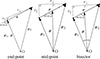 |
Fig. 1. Geometry and separation definition for end-point (left), mid-point (middle), and bisector (right) pair line-of-sight conventions. The observer is at the point ‘O’ and the two other points represent the objects of the pair. In those figures, all vectors and segments are contained in the plane determined by the vectors ⃗x and ⃗r. |
Instead of directly using a decomposition of the separation vector around the line-of-sight direction, it can be useful to express the separation vector in the associated polar basis with coordinates
 (16)
(16)
 (17)
(17)
where μ is the cosine angle between the separation and line-of-sight directions (see Fig. 1). From this we can further define the 2PCF multipole moments of the order, ℓ,
 (18)
(18)
where Lℓ(μ) is the Legendre polynomial of order ℓ. In the auto-correlation function case, there is no physically expected odd multipole signal. However, in the case of the cross-correlation between different populations, a relativistic signal can arise in the odd multipole correlation functions (e.g. Breton et al. 2019). 2PCF-GC has been built such that this type of signal can be extracted and provides in output all even and odd moments up to ℓ = 4.
Finally, an estimate of real-space clustering, namely, without the effect of redshift-space distortions, can be obtained by integrating ξ(r⊥, r∥) over r∥. This leads to the projected 2PCF
 (19)
(19)
where, in practice, the integral is definite and finite integration limits have to be defined to mitigate the effect of large uncorrelated pairs in the integral. In 2PCF-GC, both integrals in Eqs. (18) and (19) are evaluated as Riemann sums over the linearly binned anisotropic 2PCF.
2.3. Data spatial partitioning
The implementation of the 3D 2PCF estimation in Euclid uses specific data partitionings to enable an efficient estimation from the huge dataset that Euclid will produce. An overall spectroscopic sample of about 20–30 million galaxies with redshifts is expected in the completed Euclid Wide Survey (Euclid Collaboration: Mellier et al. 2025). To address this task, three efficient pair-counting algorithms have been developed, based on different data spatial partitionings: linked-list, k-d tree, and octree. They exploit the observation that, at fixed requested scale range, not all possible distinct pairs have to be computed and stored. Those data spatial partitionings allowed us to explore efficiently all pairs where the separation falls within the requested scale range and prune the exploration of irrelevant data. The purpose of developing different pair-counting methods is to have different ways of assessing the same quantity and identify the fastest and more reliable method. After the development and optimisation of the methods, we found that in the end all three are very efficient, as discussed in the next section. It is worth emphasising that those methods are exact and no approximation is involved at the pair-counting level.
2.3.1. Linked-list algorithm
The linked-list algorithm for range searching, also sometimes referred to as the chained-mesh algorithm, implements a 3D regular pixellation scheme. Our implementation builds on the work of Marulli et al. (2016) and a similar algorithm has been used in other implementations (e.g. Alonso 2012; Donoso 2019; Sinha & Garrison 2020). The data bounding volume was divided into a regular Cartesian mesh and the indexes of objects residing in each cell are stored in a list: the linked list. In practice, the elements (or nodes) of the list are not explicitly linked, instead they are stored in a vector of indexes that map to their 3D positions.
The pair counting was performed through two nested loops: a first loop goes through all cells containing objects, while the second explores the neighbouring cells whose maximum distance is below the requested maximum separation. In the inner loop, all pairs of objects are counted as in the naive nested-loop algorithm. This strategy allows the pruning of irrelevant pair counts that are outside of the required separation range. The efficiency of the algorithm depends on the cell size and mean number of object per cell. Optimally, one would like to have a cell volume corresponding to a multiple of the search sphere and the most appropriate mean number of object per cell. The latter has to be large enough to avoid having to explore too many cell-cell pairs but small enough to avoid having a too large cell volume, and in turn the pruning to be inefficient. After several trials, an optimal choice of setting the number of cells such that there are about 100 objects per cell on average is used in our implementation. Practically, this is done by first taking the maximum separation as cell size and estimating the averaged number of objects per cell. Then, the cell size is divided by the integer value that allows us to reach approximately 100 objects per cell on average.
2.3.2. k-d tree algorithm
The k-d tree range-search algorithm (Bentley 1975) is based on partitioning the set of object positions into a binary tree. Starting from the smallest axis-aligned bounding volume encompassing all data points, namely, the tree root, tree nodes are obtained by recursively dividing into two equipopulated subsets until reaching the leaves of the tree. Each subsequent partitioning forms two children nodes that contain subsets of the parent node set and in which objects are close in space. Each binary split increases by unity the depth of the tree. In the classical k-d tree, the node splitting is performed along the dimension with largest spread, at the median object position. The leaves correspond to the highest-depth nodes, when the number of objects reaches a minimum value. In our implementation, we used a minimum value of 100 objects and the sliding-midpoint method for the node splitting rule, which is more adapted for clustered objects (Maneewongvatana & Mount 1999). This choice has proven to be the most efficient.
A crucial aspect of k-d tree is that the bounding volume coordinates of each node are kept in the data structure. This information is then used to search through the tree. For the purpose of counting pairs, we use the dual-tree approach that is a generalisation of the single-tree range-search algorithm for pairs (Moore et al. 2001; Zhao 2023). The search is performed by spanning two trees simultaneously and testing each node pair recursively. Depending of the minimum and maximum distance between the tested nodes, the search can be stopped or passed through to the children nodes. This process stops when reaching the leaves. With this method, one can efficiently prune pairs, when separations are outside of the required separation range. The pair counting is effectively performed at the level of the leaves, using a nested loop going over all pairs, whose complexity goes as 𝒪(n2), where n is the number of objects in the leaves.
2.3.3. Octree algorithm
In the octree algorithm (Meagher 1980), the partitioning of the data volume is organised in a tree structure in which each internal node has exactly eight children, as opposed to two children for the k-d tree. The octree is built from the smallest cubic bounding volume encompassing all the data points. This root node is then recursively subdivided in octants, obtained by dividing the side in each of the three dimensions in two equal parts. Each subsequent partitioning increases the depth of the tree and this process stops when reaching the leave nodes. The leaves can be defined by imposing the maximum depth of the tree, or a minimum value for the number objects in the leaves. Similarly as for the k-d tree, and after several trials, we set the latter minimum value to 100 objects.
Our implementation used a hashed octree structure (Warren & Salmon 1993), where tree nodes are stored in a hash table and each node is identified by its Morton binary code (Morton 1966). This allows for the optimisation of the data structure storage and memory access, while also leading to the most optimal performance in tree traversing. Because of the regularity of the octree spatial structure, the node bounding volume coordinates can efficiently be deduced from the Morton code by using bitwise operations. This information is then used to search through the tree. The pair counting is performed similarly as for the k-d tree, by spanning two octrees simultaneously and testing each node pair recursively. Depending of the minimum and maximum distance between the tested nodes, the search can be stopped or passed through to the children nodes, and the process stops when reaching the leaves. The pair counting is performed at the level of leaves, in a similar manner as for the k-d tree.
2.4. Software architecture
The 2PCF-GC processing function is a processing element of the Euclid SGS, which carries out the entire data processing up to cosmological parameter extraction. There are ten Organisational Units (OU) within the SGS, each one having the responsibility to define, design, and validate a specific analysis of the SGS workflow. 2PCF-GC belongs to OU-Level 3 that is in charge of producing the highest-level scientific data products. The data processing within the Euclid SGS is performed in a distributed system across the Science Data Centers (SDC) from Finland, France, Germany, Italy, Netherlands, Spain, Switzerland, United Kingdom, and the United States. While most of the SDC have a High Throughput Computing (HTC) design, the underlying infrastructure can vary across SDC. For high-performance computation, as particularly required by this processing function, the overall infrastructure allows for parallelisation.
The development of the 2PCF-GC code was performed in C++11 within the framework of the Euclid SGS common tools and guidelines to ensure homogeneity in terms of development, storage, and computing, independently of the location (Frailis et al. 2019). This development followed the common Euclid Development ENvironment (EDEN), which establishes the set of libraries and associated versions to be used by any of the Euclid software and prevents inconsistencies or changes in the functionality of different libraries between development and production. 2PCF-GC was integrated in the COllaborative DEvelopment ENvironment (CODEEN), a continuous integration and delivery (CI/CD) platform that automates the building, unit testing, and distribution of all the scientific software in the SGS. The source code is stored in a Version Control System (Gitlab) and can be run through a CI/CD pipeline to be finally deployed on a distributed file system available on all SDCs. This system design allows SGS operations to be performed smoothly and efficiently across all SDC, providing the extra advantage of increased computing power and storage capacity. 2PCF-GC has been developed to run within the SGS infrastructure, but can also be run in standalone mode, which has demonstrated to be crucial for testing and validation activities.
2.4.1. Process overview
The overall 2PCF-GC processing follows four main steps as illustrated in Fig. 2. In the first step, it reads the inputs: a configuration file, data and random catalogues, and pre-computed pair counts if this option is selected in the configuration file. In pipeline mode, those catalogues are provided by the preceding processing function in the SGS pipeline chain, the SEL-ID processing function. The latter extracts a catalogue from the Euclid Wide Survey using certain selection criteria and provides it with the associated random catalogue to 2PCF-GC. The input galaxy and random catalogues are then read and decomposed into an internal spatial representation: linked-list, k-d tree, or octree, depending on the chosen pair-counting method. After building the internal data structure, the counting algorithm roams over it to identify the pairs as a function of separation. Weighted pair counts in each separation bin are stored in arrays. 2PCF-GC performs the necessary pair counts in series depending on the requested estimator. Alternatively, they can be read from input files. Those pair counts are finally combined to obtain the 2PCF estimate. At the end of the process the 2PCF and individual pair counts products are prepared and delivered in the form of FITS files (Pence et al. 2010).
 |
Fig. 2. 2PCF-GC process overview. The different boxes illustrate the different steps involved in the processing. |
2.4.2. Inputs and outputs
The inputs and outputs of 2PCF-GC are defined in the Euclid Common Data Model, which defines the format of the input and output data and metadata, and ensures the stability of interfaces between pipelines and the Euclid Archive System (EAS). The latter is the database containing all data products and metadata processed for the Euclid mission (Williams et al. 2019). The input products of 2PCF-GC are a configuration file, a set of data and random catalogues, and possible pre-computed pair counts from a previous run. The input catalogues contain the 3D spatial information of objects as well as optional statistical weights. The latter can be used for instance to up-weight or down-weight objects in pairs to account for variations in the spatial sampling of certain objects. The input celestial coordinate system can be either the equatorial Cartesian or spherical system, where in the spherical case, the radial coordinate is either a redshift or a comoving radial distance. In the case that the redshift is provided, 2PCF-GC first converts the redshift to a comoving radial distance from a provided fiducial cosmological model. After that, Cartesian coordinates are used in the pair counting. The output products are tabulated 2PCF measurements and associated pair counts. Apart from the input catalogues, through the parameter list, the configuration file allows for the specification of:
-
the correlation function estimator: auto-correlation, cross-correlation, modified auto-correlation, modified cross-correlation;
-
the correlation function type: angle-averaged ξ(r), anisotropic ξ(r⊥, r∥) and w⊥(r⊥), anisotropic ξ(r, μ) and ξℓ;
-
the pair-counting method: linked-list, k-d tree, or octree;
-
the type of binning (linear or logarithmic) and definition of bins;
-
the pair line-sight definition for ξℓ;
-
the upper limit of integration along r∥ for the projected correlation function;
-
an option to enable reusing pre-computed pair counts;
-
the number of splits of the random catalogue when using the random split option.
3. Optimisation
The main challenge in estimating the 2PCF from Euclid data is to perform pair counting from massive galaxy and random catalogues in a reasonable amount of time. Euclid scientific accuracy requirements impose a 10% accuracy relative to statistical uncertainty. This translates at estimation level into imposing a number of random catalogue objects of at least 50 times that of the galaxy catalogue, since the estimator variance depends on the number of objects in the data and random catalogues (Landy & Szalay 1993; Keihänen et al. 2019). The choice of using random catalogues with at least 50 times more objects than in the data catalogue is a formal requirement of the Euclid mission endorsed by ESA, allowing us to reach only a percent-level contribution to the 2PCF standard error from the finiteness of the random catalogue. A significant effort has been put on optimising 2PCF-GC for speed and memory consumption. This was performed by making use of optimal data spatial partitioning and pair-counting method as previously discussed, but also by implementing parallelisation and a specific treatment of random-random pair counts based on a the random split technique. We describe those two aspects in the following.
3.1. Parallelisation
The parallelisation of pair counting can be achieved straightforwardly for the three considered algorithms. For the linked-list algorithm, this is done by splitting the loop over mesh cells in chunks and performing the computation for each chunk in parallel. In the case of the k-d tree and octree algorithms, instead of starting from the tree root, the pair counting starts in parallel from all internal tree nodes at a given depth (greater than zero). In all cases, the parallel instances computes partial counts that are then summed up in order to obtain the final counts. Those parallelisation strategies have been implemented using the shared-memory Open Multi-Processing (OpenMP) application programming interface. The scaling and performance of these implementations are presented in Sect. 4.
3.2. Treatment of random-random pair counts
Random-random pair counts dominate the overall computation time of the 2PCF as it involves the largest number of pairs. A major gain in runtime can be obtained by using the so-called random split technique in the computation of those pairs. This technique, described in Keihänen et al. (2019), relies on first splitting the random catalogue in NS sub-catalogues, calculating all DRi and RRi pair counts, and finally summing up sub-catalogue pair counts to obtain the final random-random and data-random pair counts. Therefore the estimator for the 2PCF (auto-correlation case) becomes
 (20)
(20)
where
 (21)
(21)
 (22)
(22)
With this strategy the maximum number of random-random pairs to be computed is smaller by a factor of  compared to the case without random split, leading to a significant gain in computational time. An optimal NS is such that each random sub-catalogue is of the same size as the data catalogue. Keihänen et al. (2019) studied the bias and variance of the 2PCF estimator with this treatment and found that, for a random catalogue 50 times larger than the galaxy catalogue, this technique reduces the computation time by a factor of more than ten without affecting estimator variance or bias. In the following, we adopt as baseline random catalogues that have 50 times the number of galaxies in the data catalogue, and when using the random split technique, an optimal value of NS = 50. We show in the next sections that this effectively allows us to reach the accuracy requirement of Euclid.
4. Validation and performance
The testing and validation of 2PCF-GC were performed at the different stages of development of the code. 2PCF-GC has successfully passed six maturity level gates, each one involving a series of validation tests including 2PCF calculations on mock data. Significant efforts have been put in making the code meet high coding standards following the quality requirement defined by SGS. We present in this section the results from the most significant validation tests, with a focus on accuracy, runtime, and memory tests.
4.1. Benchmark catalogues
To perform benchmarks of 2PCF-GC, we made use of different sets of mock data catalogues. Each one was selected to perform a specific test and has different characteristics. We review in the following those characteristics.
-
Euclid Large Mocks: The ELM suite has been designed for studying observational systematic errors on galaxy clustering. Those are realisations of Hα-emitting galaxies in a lightcone of radius 30 deg on the sky. They are based on the Pinocchio approximate method for efficiently generating halo catalogues and lightcones (Monaco et al. 2013). Pinocchio halos are populated with emission-line galaxies using a halo occupation distribution model calibrated on the flagship galaxy mock presented in the next section. As for the flagship galaxy mock, the simulated galaxy catalogue corresponds to Hα emitters with flux above 2 × 10⁻¹⁶ erg s−1 cm−2 and distributed over the redshift range 0.9 < z < 1.8. To perform validation tests, we only considered galaxies at 0.9 < z < 1.1 in the first mock, leading to an effective volume of V = 1.5 h−3 Gpc3. Details of the ELM mocks are provided in Monaco et al. (in prep.).
-
CoxMock suite: The CoxMock suite has been designed to produce mocks for which the true 2PCF is known, and which can be produced massively in a reasonable amount of time. To do this, we used an isotropic line-point Cox process where lines of a given length are randomly placed in a periodic cubical volume and points are randomly scattered on those lines (Stoyan et al. 1995). We generated 10 000 catalogue realisations of a cube of side 1.74 h−1 Gpc containing 106 objects. For each realisation, 100 000 lines of length 800 h−1 Mpc and 1 000 000 points were drawn. More precisely, each line was drawn at random position and orientation by randomly selecting one of the endpoints inside the simulation box. Each point was then randomly placed on one line by first randomly choosing a line and second uniformly distributing it on the chosen line. If lines or points fell outside of the cube boundaries, they were mirrored by the opposite face, effectively applying periodic boundary conditions. The expected 2PCF of points in these mocks resembles a cosmological ξ(r) as it is described by a damped power-law with an index of −2 (see Sect. 4.3).
4.2. Runtimes and scaling with number of objects
We tested the runtime of 2PCF-GC with the different pair-counting algorithms and as a function of the number of objects in the catalogues. For this, we extracted four sub-catalogues with No = [104, 105, 106, 5 × 10⁶] randomly chosen objects from the ELM mock. We then built the associated random catalogues with 50 times more objects than in the data. The redshift distribution of random objects was drawn from the estimated mean distribution over 1000 mocks. Since the volume of the mock is the same, the sub-catalogues probe different number densities of objects. In this test, we considered the estimation of the multipole correlation functions in 40 linear bins in r spanning the interval [0, 200] h−1 Mpc and 200 in μ. The runtimes are obtained using a computer cluster node equipped with 32 physical central processing units (CPU) Intel(R) Xeon(R) Silver 4216 at 2.10 GHz, and by performing 5 runs with 4, 8, 16, or 32 parallel threads, except for the longest runs with No > 106 where only one run with 32 threads was performed.
Figure 3 presents the times in CPU-hour that we obtained when estimating the multipole correlation functions with the different algorithms, as a function of the number of objects. The total runtimes, denoted by 2PCF in the figure, are divided in different parts corresponding to the time spent on data structure construction, DD and RR pair counting. While the data structure construction time scales linearly with the number of objects, the DD, DR, and RR pair-counting times scale quadratically for a constant volume, as expected. Overall, the data structure construction has a subdominant contribution of one up to seven orders of magnitude smaller than pair counting. The DD, DR, and RR pair-counting times are similar for the tree-based algorithms, while the linked-list algorithm shows a steeper slope with the number of objects, that is, smaller times for low No and slightly longer times above 106 objects. The full calculation of the 2PCF is dominated by the RR counts and the overall runtimes reflect this, with the tree-based algorithms and particularly the octree performing best. Furthermore, the random split option allows us to drastically reduce the runtimes by up to a factor of 10 for a data catalogue of 5 × 10⁶ objects, as shown in Fig. 3. In that case, the 2PCF multipoles are computed in about 7 hours on 32 threads, while without this lasts 4 days. The scaling with the number of objects is slightly different for the three pair-counting algorithms. Since the individual random split sub-catalogues have approximately the same size as the data catalogue, the times are dominated by smaller-size catalogues for which the linked-list algorithm proves to be slightly faster. This is true up to approximately No = 5 × 10⁵, and at larger No the runtimes are similar for the three algorithms, with only the octree being marginally faster for 5 × 10⁶ objects. For the full 2PCF calculation, the linked-list algorithm runtimes scale very accurately as No2, while for tree-based algorithms as  in the regime of No > 105.
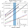 |
Fig. 3. Run times for the calculation of the multipole correlation of galaxies obtained from the ELM mock. The times are expressed in CPU-hour and as a function of the data or random catalogue size. The various symbols represent the time spent on the data structure construction, DD calculation, DR calculation, RR calculation, and the overall 2PCF runtime with and without random split option. The DR calculation times are provided as a function of the number of objects in the data catalogue and assuming a fifty times larger random catalogue. The different curves represent the runtimes obtained with the linked-list (solid), k-d tree (dashed), and octree (dotted) algorithms. The blue vertical band shows the range of expected number densities in the spectroscopic sample at redshifts within 0.9 < z < 1.8. The abscissa refers to the number of object in the data catalogue except for RR calculation where it refers to that in the random catalogue. |
The volume of the ELM mock that we used for runtime tests corresponds approximately to the volume probed spectroscopically by the Data Release 1 of Euclid in the redshift interval 0.9 < z < 1.1. We show with the vertical blue band in Fig. 3 the expected number density of galaxies over 0.9 < z < 1.8, which gives an idea of the expected runtime to measure the multipole correlation functions in the first redshift interval: about 30 min on 32 threads. It is worth noting that the runtimes also scale in an independent manner with volume and maximum scale. Up to approximately 5 millions of Hα-emitting galaxies 0.9 < z < 1.1 are expected in the spectroscopic catalogue by the end of the Euclid Wide Survey, and according to our tests, the calculation would last a bit less than a day on 32 threads using the random split option. This represents a reasonable time and meets Euclid mission requirement, given that more than 32 threads will be usable in the SDC for the actual Euclid data processing. In particular, some SDC can provide up to 128 usable parallel threads.
We compare in Fig. 4 the runtimes for the correlation function multipole moments measured by 2PCF-GC with those obtained with the publicly available Corrfunc code v2.5.3 (Sinha & Garrison 2020). In this comparison, we use the same binning configuration and input catalogues. In addition to OpenMP, Corrfunc makes use of Single Instruction Multiple Data (SIMD) parallelism that permits vectorising some operations at the CPU level. This can allow a speed-up in the pair counting from about 50% to up to a factor of 2–3 depending on the CPU used (Sinha & Garrison 2020; Zhao 2023). Because computing infrastructures can vary across Euclid SDC and the constraint on portability of the different PF, no attempt was made to include SIMD parallelism in 2PCF-GC. Therefore, for a fair comparison we only used Corrfunc without SIMD vectorisation enabled. As shown in Fig. 4, in this configuration 2PCF-GC is slightly faster than Corrfunc by up to 30%, depending on the number of objects.
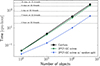 |
Fig. 4. Comparison of the runtimes for the calculation of the multipole correlation of galaxies in the ELM mocks using 2PCF-GC and Corrfunc publicly available code. |
4.3. Accuracy tests
Within the validation of 2PCF-GC, we conducted a series of tests on the accuracy of the estimated 2PCF. We tested both the absolute accuracy and relative accuracy to estimates obtained from an external software. Those tests are presented in the following.
4.3.1. Absolute accuracy
We made a comprehensive analysis that uses a series of mocks for which the underlying 2PCF is perfectly known, namely the CoxMock suite of mocks. We generated 10 000 realisations allowing us to reach extremely precise summary statistics on the 2PCF. Pons-Bordería et al. (1999) give the following expression for the 2PCF of the line-point Cox process when r ≤ L:
 (23)
(23)
where L is the line length and nL is the line number density. Due to the finite number of lines and the fact that each point is placed on a randomly chosen line, for a given point, the probability that another point falls on another line is given by 1 − 1/NL. This leads to an additional term  to the above expression for ξcox and in turn, the reference bin-averaged CoxMock isotropic correlation function becomes
 (24)
(24)
where rlow and rup are the lower and upper limits of the bin in r.
We measured the angle-averaged and multipole correlation functions in the mock realisations using 200 and 40 linear bins in r spanning the range [0, 200] h−1 Mpc and including the random split option. In those mocks there is no anisotropic clustering and we recover vanishing quadrupole and hexadecapole moments with residual random variation around zero, as expected. To quantify the accuracy on the estimation, we calculate the mean bias relative to the standard deviation Δξ/σ and mean relative bias Δξ/ξref, respectively defined as
 (25)
(25)
 (26)
(26)
where ⟨ξ(r)⟩ refers to the mean ξ(r) over the realisations, and σ corresponds to the reference statistical uncertainty in Euclid. The detailed calculation of the latter is given in Appendix A. The mean over the 10 000 realisations suppresses field stochasticity and sample variance. Both quantities are shown in Fig. 5. We find that the mean bias in the estimated correlation is extremely low, always below 10% of the statistical uncertainties for all considered scales. There are residual sample variance fluctuations, but overall we do not find any trend of bias. On closer inspection, we find that, except on scales below 10 h−1 Mpc, the mean bias is always below about 5%. Similarly, the mean relative bias is always below 1% and can reach 0.1 per cent at the smallest scales. Finally, we can also estimate the mean bias relative to the uncertainty in the CoxMocks, where σ(r) is replaced by σcox(r) in Eq. (25). This is presented in Fig. 6, where we can see that intrinsically the relative accuracy on the 2PCF is essentially always within 3% for a volume of 5.268 h−3 Gpc3.
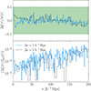 |
Fig. 5. Accuracy of the estimated real-space correlation function from the CoxMocks. While the top panel presents the mean bias relative to the standard deviation Δξ/σ, the bottom panel exhibits the absolute value of the mean relative bias |Δξ/ξref|. These estimates are obtained by averaging over 10 000 mock realisations. In the top panel, the horizontal coloured band represents ±10% of σ(r). |
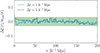 |
Fig. 6. Same as in the top panel of Fig. 5, but relative to the uncertainty in the CoxMocks. This estimate is obtained by averaging over 10 000 mock realisations. The horizontal coloured band represents ±3% of σcox(r). |
4.3.2. Relative accuracy
We further compared the standard and modified correlation function multipole moments measured by 2PCF-GC with those obtained with Corrfunc. For this test we used the Flagship Galaxy Mock v1 galaxies at 0.9 < z < 1.1 (see Sect. 5) and considered 40 linear bins in r spanning the range [0, 200] h−1 Mpc. We used the same catalogues as input of 2PCF-GC and Corrfunc. The difference in the monopole, quadrupole, and hexadecapole relative to the expected statistical error expected in Euclid, are presented in Fig. 7. For each multipole moment, the relative accuracy between the two estimates is of the order of the machine precision, both for the standard and modified 2PCF. In the modified 2PCF estimation, the reconstructed data and auxiliary random catalogues were obtained using the recSym BAO reconstruction algorithm, as detailed in Sarpa et al. (in prep.). The latter reconstruction algorithm uses Lagrangian Perturbation Theory to predict bulk-flow displacements and substracts them from the random point and galaxy positions (Padmanabhan et al. 2012; Burden et al. 2015).
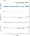 |
Fig. 7. Difference in the monopole (top panel), quadupole (central panel), and hexadecapole (bottom panel) moments of the standard (ξℓ) and modified (ξℓm) correlation function between the 2PCF-GC and Corrfunc estimates, relative to the standard deviation. These measurements are obtained from a single mock realisation. |
Finally, we tested the impact of using the random split option on the accuracy of the estimated 2PCF multipole moments. For this, we compared the measurements obtained in the same mock catalogue with the same setup as before while using or not this option. The difference in the monopole, quadrupole, and hexadecapole relative to the expected statistical error is shown in Fig. 8.
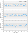 |
Fig. 8. Impact of the random split option on the accuracy of the measured 2PCF. The curve shows the difference in the monopole (top panel), quadupole (central panel), and hexadecapole (bottom panel) moments of the correlation function, while using or not the random split option with NS = 50. The shaded areas represent the regions encompassing respectively 10% and 20% of the expected statistical uncertainty. These measurements are obtained from a single mock realisation. |
The results show that the random split option with NS = 50 introduces random errors below 10% of the statistical uncertainties for all considered scales and no systematic error. It is worth emphasising that those uncertainties can be reduced by reducing the number of random splits, at the expense of longer runtimes.
Overall, these tests validates 2PCF-GC accuracy and the choice of using 50 times more random points than objects in the data catalogue and the usage of the random split option. We would like to emphasise that, even if not presented here, we also performed other accuracy and consistency tests on the cross-correlation function, and in all cases, we found similar, very good accuracies. This includes for instance consistency tests of the cross-correlation function where the two data catalogues are taken as two random sub-samples of a data catalogue. 2PCF-GC has been used to estimate cross-correlation functions in Risso et al. (in prep.).
4.4. Memory usage
The random-access memory (RAM) usage of 2PCF-GC is dominated by the storage of the input data and random object positions and weights. Furthermore, the memory required to process the data can increase depending on the amount of information comprised by the linked-list or tree structures. Although object properties are not directly copied into the spatial partitioning structures, additional metadata associated with the latter must be stored in memory. The linked-list structure, which comprises an ordered array of integers that convey information about the objects present in each cell, formally requires the least memory. The tree structures generally require the storage of more information. Each tree node contains several pieces of information including the coordinates of the bounding volume associated with the node, the indices of the objects contained in the node, and pointers to child nodes. This increases the amount of information to be stored in memory. However, the use of hash tables allows the pointer information to be removed, and in the case of the octree, the Morton code associated with each node allows the bounding volume coordinates to be computed directly, thus saving further memory.
In Fig. 9 we present estimates of the memory usage of 2PCF-GC from the ELM mock, both accounting for the RAM resident set size and swap space, for the three methods and as a function of the number of objects in the data catalogue. The memory usage increases with the number of objects and the storage of the input catalogues dominates the overall budget. The linked-list method tends to use less memory, but thanks to the implementation of hash tables for both k-d tree and octree, the memory usage is only marginally larger for the latter methods. Overall, for a data catalogue of five million objects and 50 times more in the random catalogue, about 19 GB of memory is required. In the case where the random split option is used, only a fraction of the random catalogue needs to be stored in memory at a time and thus the necessary memory for storing the random object information is significantly lower. In that case only about 0.9 GB of memory is required for a data catalogue containing five million objects.
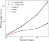 |
Fig. 9. Memory usage as function of the number of objects in the data catalogue, for the considered data partitionings and while using or not the random split option. The different lines shows the results for the different pair-counting methods, while the different symbols indicate whether or not the random split option is used. |
5. Expectations for Euclid Wide Survey
We present in this section some forecasts on 2PCF estimation and showcase some interesting features of 2PCF-GC using a realistic full-sky mock catalogue of the Euclid Wide Survey. We made use of the Flagship Galaxy Mock (FGM) v2.1 (Carretero et al. 2017; Tallada et al. 2020), which has been constructed from the Flagship 2 N-body simulation by populating dark matter halos with emission-line galaxies as described in Euclid Collaboration: Castander et al. (2025). A sub-sample of the galaxies with an Hα flux greater than 2 × 10⁻¹⁶ erg s−1 cm−2 and a redshift in the range 0.9 < z < 1.8 has been extracted, which represents the targeted galaxies for the spectroscopic sample of the Euclid Wide Survey. The mock consist of a light-cone covering an octant of the sky, and for the purpose of performing realistic forecasts, we replicated the octant in order to have full-sky catalogue. We note that this procedure does not introduce spurious clustering features on the scales smaller than 200 h−1 Mpc, which are of interest for our analysis. This mock represents current most realistic expectation for the intrinsic clustering of Hα-emitting galaxies in the Euclid Wide Survey available within the Euclid collaboration.
5.1. Galaxy two-point correlation function across survey timeline
To illustrate the performance of 2PCF-GC and provide forecasts on the expected measured 2PCF at different stages of Euclid observations, we estimated the correlation function multipole moments in the FGM after 1, 3, and 6 years of observations, as defined in the Euclid Reference Survey3 (Euclid Collaboration: Scaramella et al. 2022). The angular extent of year 1, year 3, and year 6 observations as defined in the Euclid Reference Survey is presented in Fig. 10. We defined four redshift intervals: 0.9 < z < 1.1, 1.1 < z < 1.3, 1.3 < z < 1.5, 1.5 < z < 1.8, as used for Euclid cosmological forecasts (e.g. Euclid Collaboration: Blanchard et al. 2020).
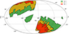 |
Fig. 10. Sky coverage of Euclid Wide Field after one, three, and six years of observations, as defined in the Euclid Reference Survey (Euclid Collaboration: Scaramella et al. 2022). |
The correlation function monopole, quadrupole, and hexadecapole are presented in Figs. 11, 12, and 13, respectively. Even if these measurements are extracted from a specific mock realisation of the observable universe, with its own sample variance, it gives a sense of the improvement on the estimation of the correlation function and high precision recovered after 6 years of observation. In particular, one can see from the monopole that the BAO peak in the lowest redshift interval is not very pronounced with the first year coverage, while at the end of the survey, the signal is much more significant. On scales beyond 100 h−1 Mpc, we can see significant variations of the amplitude between year 1 and year 6, which can be attributed to sample variance, the fact that the over-density distribution associated with galaxies differs significantly. Similar trends are seen in the quadrupole and hexadecapole. Particularly for the latter, which is the most uncertain, one can see that the end-of-survey amplitude tends to vanish on large scales, as expected.
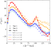 |
Fig. 11. Monopole correlation function estimated from the FGM mock for galaxies with Hα flux above 2 × 10⁻¹⁶ erg s−1 cm−2 at different epochs of observations. The different colours show the monopole in the redshift intervals: 0.9 < z < 1.1, 1.1 < z < 1.3, 1.3 < z < 1.5, 1.5 < z < 1.8. |
5.2. Impact of pair line-of-sight definition
In order to showcase the capabilities of 2PCF-GC, we estimated the multipole correlation functions in the FGM using the mid-point and end-point line-of-sight definition. Even if the estimator assumes the local plane-parallel approximation, the choice of the line-of-sight definition has different sensitivity to wide-angle effects. From its maximally-symmetric properties, the mid-point definition minimises the latter effects, while the end-point definition is more affected (e.g. Reimberg et al. 2016; Beutler et al. 2019). This can be seen in Fig. 14, which shows the absolute difference between using the mid-point and end-point definitions in the estimator, for the monopole and quadrupole correlation functions in the year 6 dataset. In particular, it is instructive to see that the absolute difference has no strong redshift dependence in the monopole. This difference remains within the 1σ statistical error expected in the completed Euclid Wide Survey at r < 100 h−1 Mpc, shown with the dotted line in the figure. In the quadrupole instead, the effect can be more significant. In the two highest redshift intervals, the difference goes beyond the expected 2σ statistical error on the quadrupole. Overall, these results gives some insights on the typical wide-angle effects expected on large scales in the final Euclid Wide Survey sample when using the end-point line-of-sight definition.
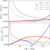 |
Fig. 14. Impact of the choice of pair line-of-sight definition on the estimated monopole (upper panel) and quadrupole (lower panel) correlation functions in FGM mock. The curves show the absolute value of the difference between using mid-point and end-point definitions in the estimator for the monopole and quadrupole correlation functions. The different colours show this quantity for the redshift intervals: 0.9 < z < 1.1, 1.1 < z < 1.3, 1.3 < z < 1.5, 1.5 < z < 1.8. The dotted (dashed) line shows the expected 1σ (2σ) statistical error in the completed Euclid Wide Survey in the interval 1.1 < z < 1.3. |
5.3. Integral constraint
The normalisation of the pair counts to the observed number of galaxies in the LS estimator imposes a constraint on the integral of the observed over-density field in the survey, which is that the latter vanishes. However, because of the finite size of the sample, the integral over the observed over-density field does not necessarily vanish and this leads to biasing negatively the correlation function on large scales (Peebles 1980). This effect, commonly referred to as the integral constraint, is particular important for small surveys. In the Euclid Wide Survey, which will be among the largest spectroscopic survey of galaxies, the expected effect is very small. Nonetheless, given the unprecedented statistical precision in the correlation function measurements expected in Euclid, it is important to assess the level and scales at which the integral constraint can impact the measurements.
The integral constraint introduces a bias on the observed correlation function and, at first order, the model for the latter is (e.g. de Mattia & Ruhlmann-Kleider 2019):
 (27)
(27)
where ξ(⃗r) is the theoretical correlation function,
 (28)
(28)
δ(⃗x) is the over-density field, W(⃗x) is the survey window function, and ∫Vd3x denotes an integral over the survey volume. The leading integral-constraint term in the correlation function is (de Mattia & Ruhlmann-Kleider 2019):
 (29)
(29)
where the survey window function correlation function and associated multipole moments are
 (30)
(30)
 (31)
(31)
respectively. In the previous equations, ⃗Δ denotes a separation vector. By expanding Eq. (27) in multipole moments, one can see that the constant integral constraint term will only survive in the monopole correlation function. Moreover, by realising that the survey window function correlation function is directly related to random-random counts by RR(⃗Δ)∝Δ2𝒲(⃗Δ) (Wilson et al. 2017), Eq. (29) can be rewritten as
 (32)
(32)
 (33)
(33)
where in Eq. (33) the continuous integral is approximated by a discrete sum over bins4Δi, and Nb is the number of bins. In the previous equation, RRℓ is defined as
 (34)
(34)
Therefore, by using Eq. (33) we can directly estimate the impact of the integral constraint from the random-random pair counts and a prior knowledge on the true underlying multipole correlation functions.
We compute the integral constraint correction expected in Euclid from Eq. (33) by using the RR counts estimated by 2PCF-GC and performing the discrete sum up to Δ = 1000 h−1 Mpc. The correlation function multipoles in the integral are taken from the measured multipole (symbols) or by using an analytical model for the redshift-space multipole correlation functions. The latter was obtained by fitting the FGM measurements with most accurate full-shape models for the correlation function multipole moments, as described in Kärcher et al. (in prep.). The main advantages of using a model ξℓ is to have a prediction up to the largest scales and that is not itself affected by the integral constraint. Overall, we found values of ⟨ϵ2⟩ varying within (3–8) × 10−5, depending on the epoch of observations and the redshift interval.
We present in Fig. 15 the leading integral-constraint term ⟨ϵ2⟩ estimated from the FGM, for the different redshift intervals and observing periods considered. We can see that the impact of the integral constraint depends on the size of the surveyed volume and the considered redshift interval. The effect is the most important at year 1 for all redshift intervals, as expected. At year 3 and then year 6, the effect diminishes. The predictions obtained from using the analytical ξℓ in the integral constraint calculation for year 6 are shown in Fig. 15 with the solid curves. Those predictions are perfectly in line with those obtained from taking the measured ξℓ, although on the largest scales, they provide more robust predictions as they are not affected by sample variance. In essentially all cases, the effect remains within the 1σ statistical uncertainty expected at year 6, as shown with the dotted line in Fig. 15. In future Euclid cosmological analyses, this effect can be straightforwardly accounted for at likelihood level, when confronting measurements to model predictions, or simply neglected if the analysis is limited to scales below about r = 150 h−1 Mpc.
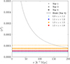 |
Fig. 15. Impact of the integral constraint on the monopole correlation function in the Euclid Wide Survey. The curves with the different different symbols show the leading integral-constraint term ⟨ϵ2⟩, after 1, 3, and 6 years of observation respectively. The solid curves show the same quantity for year 6 observations, but when the integral constraint effect is derived from a model correlation function. The different colours show this quantity for the redshift intervals: 0.9 < z < 1.1, 1.1 < z < 1.3, 1.3 < z < 1.5, 1.5 < z < 1.8. The dotted curves delineate the expected 1σ statistical uncertainty on the monopole correlation function in the completed Euclid Wide Survey in the interval 1.1 < z < 1.3. |
As a final remark, we note that we did not consider here the impact of the sample purity and completeness, as well as possible radial integral constraint effects (de Mattia & Ruhlmann-Kleider 2019), which are beyond the scope of this paper and are the subject of forthcoming Euclid Collaboration papers.
6. Conclusions
This paper describes the development and validation of the processing function of the Science Ground Segment for estimating the 3D 2PCF, as part of the Euclid mission. The methodology employed in the software is both robust and effective. The data handling process has been optimised through innovative spatial partitioning strategies, which drastically reduce computation time while maintaining high accuracy. These optimisations are crucial for meeting the Euclid mission’s stringent scientific requirement, which demand speed and precision. This involves advanced algorithms such as k-d tree, octree, and linked-list, employed for pair counting and that ensure an efficient, yet exact, estimation of the 2PCF. The other key feature of the software is its optimisation and parallelisation capabilities. By leveraging the OpenMP application programming interface, the software achieves significant improvements in computational efficiency. These methods are indispensable for managing the extensive and complex dataset anticipated from the Euclid survey, which involves billions of galaxy pairs.
The software has undergone extensive validation using a variety of mock galaxy catalogues, which were designed to simulate the conditions and challenges of Euclid survey data. Rigorous tests have demonstrated that the software can handle the anticipated data volume and complexity, ensuring that the Euclid mission’s scientific goals can be met. The validation process has confirmed the software’s high accuracy and reliability in estimating the 2PCF, leading to an accuracy below that required by the Euclid mission. Moreover, the software’s integration into the Euclid SGS pipeline exemplifies its readiness for large-scale deployment and its pivotal role in the mission’s data processing framework for the production of highest-level scientific products for cosmology. This integration ensures that the vast amount of data collected by the Euclid mission can be processed efficiently.
We have presented forecasts of 2PCF-GC performance in measuring the 2PCF at different stages of the Euclid Wide Survey. These forecasts are based on a realistic mock dataset and illustrated the robustness and efficiency in estimating the 2PCF. This mock dataset has also allowed us to investigate the impact of different pair line-of-sight definitions on the estimation of the multipole correlation functions, highlighting differences in sensitivity to wide-angle effects over the scales that will be reached by Euclid after six years of observations. We found that deviations in the monopole and quadrupole correlation functions are less than 5% below 100 h−1 Mpc, but can exceed 25% at larger scales. We have also estimated the integral constraint bias affecting Euclid Wide Survey measurements. While this is expected to be minimal in the Euclid Wide Survey, due to the unprecedented precision required in the Euclid measurements, the assessment of the magnitude and extent of the integral constraint effect remains critical. Using both measured and analytically modelled multipole correlation functions, we estimated that the integral constraint effect is of the order of 5 × 10⁻⁵, depending on the redshift interval and observing epoch considered. Our results indicate that the effect is most pronounced in the first year of the survey, reaching 10% at the BAO scale and up to 30% at 200 h−1 Mpc, but it diminishes in subsequent years. Nonetheless, future works will need to consider additional factors in the estimation of the 2PCF, such as sample purity, completeness, and potential radial integral constraint effects, which are beyond the scope of this paper. In particular, a first assessment of the impact of expected redshift errors on the 2PCF indicate that the results shown in this paper should be considered optimistic (Risso et al., in prep.).
This is the 2PCF as a function of the norm of the separation vector.
Alternatively, one can define r∥ = |⃗x2|−|⃗x1|, where in that case, there is no explicit need to define a pair line-of-sight vector.
In this analysis we use the Euclid Reference Survey rsd2024A.
Formally, here the bins in Δ need to be equally spaced.
Acknowledgments
The authors would like to thank Jean-Charles Lambert for his help in using and extracting reliable computational measures from the LAM computer cluster. This work was supported by the ASI/INAF agreement n. 2018-23-HH.0 “Scientific activity for Euclid mission, Phase D”, the MIUR, PRIN 2017 research grant ‘From Darklight to DM: understanding the galaxy/matter connection to measure the Universe’ and the INFN project “InDark”. FM acknowledges the financial contribution from the grant PRIN-MUR 2022 20227RNLY3 ‘The concordance cosmological model: stress-tests with galaxy clusters’ supported by Next Generation EU and from the grant ASI n. 2024-10-HH.0 ‘Attività scientifiche per la missione Euclid – fase E’. This work has made use of CosmoHub. CosmoHub is developed and maintained by PIC, IFAE, CIEMAT, in collaboration with ICE-CSIC. It is partially financed by the European Union NextGenerationEU(PRTR-C17.I1) and by Generalitat de Catalunya, as well as by the grant EQC2021-007479-P funded by MCIN/AEI/10.13039/501100011033 and by the “European Union NextGenerationEU/PRTR”. The Euclid Consortium acknowledges the European Space Agency and a number of agencies and institutes that have supported the development of Euclid, in particular the Agenzia Spaziale Italiana, the Austrian Forschungsförderungsgesellschaft funded through BMK, the Belgian Science Policy, the Canadian Euclid Consortium, the Deutsches Zentrum für Luft- und Raumfahrt, the DTU Space and the Niels Bohr Institute in Denmark, the French Centre National d’Etudes Spatiales, the Fundação para a Ciência e a Tecnologia, the Hungarian Academy of Sciences, the Ministerio de Ciencia, Innovación y Universidades, the National Aeronautics and Space Administration, the National Astronomical Observatory of Japan, the Netherlandse Onderzoekschool Voor Astronomie, the Norwegian Space Agency, the Research Council of Finland, the Romanian Space Agency, the State Secretariat for Education, Research, and Innovation (SERI) at the Swiss Space Office (SSO), and the United Kingdom Space Agency. A complete and detailed list is available on the Euclid web site (https://www.euclid-ec.org).
References
- Alam, S., Aubert, M., Avila, S., et al. 2021, Phys. Rev. D, 103, 083533 [NASA ADS] [CrossRef] [Google Scholar]
- Alonso, D. 2012, arXiv e-prints [arXiv:1210.1833] [Google Scholar]
- Amendola, L., Appleby, S., Avgoustidis, A., et al. 2018, Liv. Rev. Relat., 21, 2 [Google Scholar]
- Bentley, J. L. 1975, Commun. ACM, 18, 509 [CrossRef] [Google Scholar]
- Beutler, F., Castorina, E., & Zhang, P. 2019, JCAP, 03, 040 [Google Scholar]
- Breton, M.-A., Rasera, Y., Taruya, A., Lacombe, O., & Saga, S. 2019, MNRAS, 483, 2671 [NASA ADS] [CrossRef] [Google Scholar]
- Burden, A., Percival, W. J., & Howlett, C. 2015, MNRAS, 453, 456 [NASA ADS] [CrossRef] [Google Scholar]
- Carretero, J., Tallada, P., Casals, J., et al. 2017, in Proceedings of the European Physical Society Conference on High Energy Physics. 5–12 July, 488 [Google Scholar]
- de Mattia, A., & Ruhlmann-Kleider, V. 2019, JCAP, 08, 036 [Google Scholar]
- Donoso, E. 2019, MNRAS, 487, 2824 [NASA ADS] [CrossRef] [Google Scholar]
- Euclid Collaboration (Blanchard, A., et al.) 2020, A&A, 642, A191 [NASA ADS] [CrossRef] [EDP Sciences] [Google Scholar]
- Euclid Collaboration (Scaramella, R., et al.) 2022, A&A, 662, A112 [NASA ADS] [CrossRef] [EDP Sciences] [Google Scholar]
- Euclid Collaboration (Castander, F., et al.) 2025, A&A, 697, A5 [Google Scholar]
- Euclid Collaboration (Jahnke, K., et al.) 2025, A&A, 697, A3 [Google Scholar]
- Euclid Collaboration (Mellier, Y., et al.) 2025, A&A, 697, A1 [Google Scholar]
- Feldman, H. A., Kaiser, N., & Peacock, J. A. 1994, ApJ, 426, 23 [Google Scholar]
- Frailis, M., Belikov, A., Benson, K., et al. 2019, in Astronomical Data Analysis Software and Systems XXVI, eds. M. Molinaro, K. Shortridge, & F. Pasian, Astronomical Society of the Pacific Conference Series, 521, 612 [Google Scholar]
- Grieb, J. N., Sánchez, A. G., Salazar-Albornoz, S., & Dalla Vecchia, C. 2016, MNRAS, 457, 1577 [NASA ADS] [CrossRef] [Google Scholar]
- Guzzo, L., Pierleoni, M., Meneux, B., et al. 2008, Nature, 451, 541 [Google Scholar]
- Kaiser, N. 1987, MNRAS, 227, 1 [Google Scholar]
- Keihänen, E., Kurki-Suonio, H., Lindholm, V., et al. 2019, A&A, 631, A73 [NASA ADS] [CrossRef] [EDP Sciences] [Google Scholar]
- Kerscher, M. 1999, A&A, 343, 333 [NASA ADS] [Google Scholar]
- Landy, S. D., & Szalay, A. S. 1993, ApJ, 412, 64 [Google Scholar]
- Maneewongvatana, S., & Mount, D. 1999, Center for Geometric Computing 4th Annual Workshop on Computational Geometry [Google Scholar]
- Marulli, F., Veropalumbo, A., & Moresco, M. 2016, Astron. Comput., 14, 35 [Google Scholar]
- Meagher, D. 1980, Octree Encoding: a New Technique for the Representation, Manipulation and Display of Arbitrary 3-D Objects by Computer (Rensselaer Polytechnic Institute. Image Processing Laboratory and Meagher, D.J.R.) [Google Scholar]
- Monaco, P., Sefusatti, E., Borgani, S., et al. 2013, MNRAS, 433, 2389 [NASA ADS] [CrossRef] [Google Scholar]
- Moore, A. W., Connolly, A., Genovese, C., et al. 2001, MPA/ESO/MPE Joint Astronomy Conference: Mining the Sky (ESO Astrophysics Symposia European Southern Observatory), 71 [Google Scholar]
- Morton, G. 1966, A Computer Oriented Geodetic Data Base and a New Technique in File Sequencing (International Business Machines Company) [Google Scholar]
- Padmanabhan, N., Xu, X., Eisenstein, D. J., et al. 2012, MNRAS, 427, 2132 [Google Scholar]
- Paviot, R., de la Torre, S., de Mattia, A., et al. 2022, MNRAS, 512, 1341 [NASA ADS] [CrossRef] [Google Scholar]
- Peebles, P. J. E. 1980, The large-scale structure of the universe (Princeton University Press) [Google Scholar]
- Pence, W. D., Chiappetti, L., Page, C. G., Shaw, R. A., & Stobie, E. 2010, A&A, 524, A42 [NASA ADS] [CrossRef] [EDP Sciences] [Google Scholar]
- Pons-Bordería, M.-J., Martínez, V. J., Stoyan, D., Stoyan, H., & Saar, E. 1999, ApJ, 523, 480 [Google Scholar]
- Reimberg, P., Bernardeau, F., & Pitrou, C. 2016, JCAP, 2016, 048 [CrossRef] [Google Scholar]
- Samushia, L., Branchini, E., & Percival, W. J. 2015, MNRAS, 452, 3704 [Google Scholar]
- Sinha, M., & Garrison, L. H. 2020, MNRAS, 491, 3022 [Google Scholar]
- Stoyan, D., Kendall, W., & Mecke, J. 1995, Stochastic Geometry and Its Applications, Inorganic Chemistry (Wiley) [Google Scholar]
- Tallada, P., Carretero, J., Casals, J., et al. 2020, Astron. Comput., 32, 100391 [Google Scholar]
- Warren, M. S., & Salmon, J. K. 1993, in Proceedings of the 1993 ACM/IEEE Conference on Supercomputing, Supercomputing ’93 (New York, NY, USA: Association for Computing Machinery), 12 [Google Scholar]
- Williams, O. R., Begeman, K., Boxhoorn, D., et al. 2019, in Astronomical Data Analysis Software and Systems XXVI, eds. M. Molinaro, K. Shortridge, & F. Pasian, Astronomical Society of the Pacific Conference Series, 521, 120 [Google Scholar]
- Wilson, M. J., Peacock, J. A., Taylor, A. N., & de la Torre, S. 2017, MNRAS, 464, 3121 [Google Scholar]
- Zhao, C. 2023, A&A, 672, A83 [NASA ADS] [CrossRef] [EDP Sciences] [Google Scholar]
Appendix A: Reference statistical uncertainty on the multipole two-point correlation functions in Euclid
The expected statistical uncertainty on the multipole 2PCF is based on the expected Euclid survey characteristics, number density, and clustering of observed Hα-emitting galaxies. Based on the assumptions detailed in Table 1–3 of Euclid Collaboration: Blanchard et al. (2020), 4 redshift intervals have been considered for which the observed volume, galaxy mean number density, and galaxy linear bias are given in Table A.1. With this information and a theoretical prediction for the matter power spectrum, we can calculate the expected Gaussian covariance matrix for the galaxy correlation function monopole, quadrupole, and hexadecapole using the method of Grieb et al. (2016). For the purpose of testing the accuracy on the 2PCF, we considered the case of the interval at 1.1 < z < 1.3 as representative of Euclid. The standard deviations σ0(r), σ2(r), and σ4(r) were then obtained by taking the square root of the diagonal elements of the covariance matrices of ξ0(r), ξ2(r), and ξ4(r), respectively. We assumed σ(r) = σ0(r), where σ(r) is associated with the real-space 2PCF. Those reference uncertainties are shown in Fig. A.1.
Specifications of the 4 spectroscopic galaxy samples used as baseline for Euclid forecasts (Euclid Collaboration: Blanchard et al. 2020). The table lists the redshift interval, observed volume, galaxy mean number density  , and galaxy linear bias b.
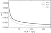 |
Fig. A.1. Reference statistical 1σ uncertainty on the monopole, quadrupole, and hexadecapole 2PCF for the completed Euclid Wide Survey. |
All Tables
Specifications of the 4 spectroscopic galaxy samples used as baseline for Euclid forecasts (Euclid Collaboration: Blanchard et al. 2020). The table lists the redshift interval, observed volume, galaxy mean number density , and galaxy linear bias b.
All Figures
|
Fig. 1. Geometry and separation definition for end-point (left), mid-point (middle), and bisector (right) pair line-of-sight conventions. The observer is at the point ‘O’ and the two other points represent the objects of the pair. In those figures, all vectors and segments are contained in the plane determined by the vectors ⃗x and ⃗r. |
| In the text | |
|
Fig. 2. 2PCF-GC process overview. The different boxes illustrate the different steps involved in the processing. |
| In the text | |
|
Fig. 3. Run times for the calculation of the multipole correlation of galaxies obtained from the ELM mock. The times are expressed in CPU-hour and as a function of the data or random catalogue size. The various symbols represent the time spent on the data structure construction, DD calculation, DR calculation, RR calculation, and the overall 2PCF runtime with and without random split option. The DR calculation times are provided as a function of the number of objects in the data catalogue and assuming a fifty times larger random catalogue. The different curves represent the runtimes obtained with the linked-list (solid), k-d tree (dashed), and octree (dotted) algorithms. The blue vertical band shows the range of expected number densities in the spectroscopic sample at redshifts within 0.9 < z < 1.8. The abscissa refers to the number of object in the data catalogue except for RR calculation where it refers to that in the random catalogue. |
| In the text | |
|
Fig. 4. Comparison of the runtimes for the calculation of the multipole correlation of galaxies in the ELM mocks using 2PCF-GC and Corrfunc publicly available code. |
| In the text | |
|
Fig. 5. Accuracy of the estimated real-space correlation function from the CoxMocks. While the top panel presents the mean bias relative to the standard deviation Δξ/σ, the bottom panel exhibits the absolute value of the mean relative bias |Δξ/ξref|. These estimates are obtained by averaging over 10 000 mock realisations. In the top panel, the horizontal coloured band represents ±10% of σ(r). |
| In the text | |
|
Fig. 6. Same as in the top panel of Fig. 5, but relative to the uncertainty in the CoxMocks. This estimate is obtained by averaging over 10 000 mock realisations. The horizontal coloured band represents ±3% of σcox(r). |
| In the text | |
|
Fig. 7. Difference in the monopole (top panel), quadupole (central panel), and hexadecapole (bottom panel) moments of the standard (ξℓ) and modified (ξℓm) correlation function between the 2PCF-GC and Corrfunc estimates, relative to the standard deviation. These measurements are obtained from a single mock realisation. |
| In the text | |
|
Fig. 8. Impact of the random split option on the accuracy of the measured 2PCF. The curve shows the difference in the monopole (top panel), quadupole (central panel), and hexadecapole (bottom panel) moments of the correlation function, while using or not the random split option with NS = 50. The shaded areas represent the regions encompassing respectively 10% and 20% of the expected statistical uncertainty. These measurements are obtained from a single mock realisation. |
| In the text | |
|
Fig. 9. Memory usage as function of the number of objects in the data catalogue, for the considered data partitionings and while using or not the random split option. The different lines shows the results for the different pair-counting methods, while the different symbols indicate whether or not the random split option is used. |
| In the text | |
|
Fig. 10. Sky coverage of Euclid Wide Field after one, three, and six years of observations, as defined in the Euclid Reference Survey (Euclid Collaboration: Scaramella et al. 2022). |
| In the text | |
|
Fig. 11. Monopole correlation function estimated from the FGM mock for galaxies with Hα flux above 2 × 10⁻¹⁶ erg s−1 cm−2 at different epochs of observations. The different colours show the monopole in the redshift intervals: 0.9 < z < 1.1, 1.1 < z < 1.3, 1.3 < z < 1.5, 1.5 < z < 1.8. |
| In the text | |
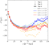 |
Fig. 12. Same as Fig. 11, but for the quadrupole correlation function. |
| In the text | |
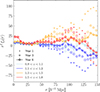 |
Fig. 13. Same as Fig. 11, but for the hexadecapole correlation function. |
| In the text | |
|
Fig. 14. Impact of the choice of pair line-of-sight definition on the estimated monopole (upper panel) and quadrupole (lower panel) correlation functions in FGM mock. The curves show the absolute value of the difference between using mid-point and end-point definitions in the estimator for the monopole and quadrupole correlation functions. The different colours show this quantity for the redshift intervals: 0.9 < z < 1.1, 1.1 < z < 1.3, 1.3 < z < 1.5, 1.5 < z < 1.8. The dotted (dashed) line shows the expected 1σ (2σ) statistical error in the completed Euclid Wide Survey in the interval 1.1 < z < 1.3. |
| In the text | |
|
Fig. 15. Impact of the integral constraint on the monopole correlation function in the Euclid Wide Survey. The curves with the different different symbols show the leading integral-constraint term ⟨ϵ2⟩, after 1, 3, and 6 years of observation respectively. The solid curves show the same quantity for year 6 observations, but when the integral constraint effect is derived from a model correlation function. The different colours show this quantity for the redshift intervals: 0.9 < z < 1.1, 1.1 < z < 1.3, 1.3 < z < 1.5, 1.5 < z < 1.8. The dotted curves delineate the expected 1σ statistical uncertainty on the monopole correlation function in the completed Euclid Wide Survey in the interval 1.1 < z < 1.3. |
| In the text | |
|
Fig. A.1. Reference statistical 1σ uncertainty on the monopole, quadrupole, and hexadecapole 2PCF for the completed Euclid Wide Survey. |
| In the text | |
Current usage metrics show cumulative count of Article Views (full-text article views including HTML views, PDF and ePub downloads, according to the available data) and Abstracts Views on Vision4Press platform.
Data correspond to usage on the plateform after 2015. The current usage metrics is available 48-96 hours after online publication and is updated daily on week days.
Initial download of the metrics may take a while.