| Issue |
A&A
Volume 700, August 2025
|
|
|---|---|---|
| Article Number | A163 | |
| Number of page(s) | 14 | |
| Section | Stellar structure and evolution | |
| DOI | https://doi.org/10.1051/0004-6361/202553980 | |
| Published online | 15 August 2025 | |
Inferring the efficiency of convective-envelope overshooting in red giant branch stars
1
Department of Physics & Astronomy “Augusto Righi”, University of Bologna, Via Gobetti 93/2, 40129 Bologna, Italy
2
INAF-Astrophysics and Space Science Observatory of Bologna, Via Gobetti 93/3, 40129 Bologna, Italy
3
INAF-Astronomic Observatory of Padova, vicolo dell’Osservatorio 5, 35122 Padova, Italy
4
Institute of Physics, École Polytechnique Fédérale de Lausanne (EPFL), Observatoire de Sauverny, 1290 Versoix, Switzerland
⋆ Corresponding author: This email address is being protected from spambots. You need JavaScript enabled to view it.
Received:
31
January
2025
Accepted:
24
June
2025
Abstract
The understanding of mixing processes in stars is crucial to improving our knowledge of the chemical abundances in stellar photospheres and their variation with evolutionary phase. This is fundamental for many astrophysical issues on all scales, ranging from stellar evolution to the chemical composition, formation, and evolution of stellar clusters and galaxies. Among these processes, convective-envelope overshooting is in dire need of a systematic calibration and comparison with predictions from multi-dimensional hydrodynamical simulations. The red giant branch bump (RGBb) is an ideal calibrator of overshooting processes, since its luminosity depends on the maximum depth reached by the convective envelope after the first dredge-up. Indeed, a more efficient overshooting produces a discontinuity in the hydrogen mass-fraction profile deeper in the stellar interior and consequently a less luminous RGBb. In this work, we calibrated the overshooting efficiency by comparing the RGBb location predicted by stellar models with observations of stellar clusters with HST and Gaia photometry, as well as solar-like oscillating giants in the Kepler field. We explored the metallicity range between −2.02 dex and +0.35 dex and found overshooting efficiencies ranging from 0.009−0.016+0.015 to 0.062−0.015+0.017. In particular, we found that the overshooting efficiency decreases linearly with [M/H], with a slope of ( − 0.010 ± 0.006) dex−1. We suggest a possible explanation for this trend, linking it to the efficiency of turbulent entrainment at different metallicities.
Key words: stars: interiors / stars: low-mass / stars: oscillations
© The Authors 2025
 Open Access article, published by EDP Sciences, under the terms of the Creative Commons Attribution License (https://creativecommons.org/licenses/by/4.0), which permits unrestricted use, distribution, and reproduction in any medium, provided the original work is properly cited.
This article is published in open access under the Subscribe to Open model. This email address is being protected from spambots. You need JavaScript enabled to view it. to support open access publication.
1. Introduction
Despite the fact that current stellar models are highly sophisticated and allow us to simulate the lives of stars from the pre-main sequence (PMS) to their final evolution stages, there are still some open questions regarding their internal structure, such as the efficiency of mixing processes beyond convective boundaries. In particular, the understanding of convective-envelope overshooting in red giant branch (RGB) stars could contribute to the explanation of photospheric abundances, for example leading to a more accurate calibration of masses (hence ages) of low-mass stars based on the carbon-to-nitrogen ratio (Salaris et al. 2015; Hasselquist et al. 2019; Jofré 2021), or to a better understanding of lithium depletion in solar-like stars (Baraffe et al. 2017, 2021). This phenomenon has also been extensively studied in the Sun (to better constrain its structure) by comparing the predictions of the models with helioseismic data (Christensen-Dalsgaard et al. 2011; Baraffe et al. 2022; Zhang et al. 2022; Buldgen et al. 2025).
Until now, overshooting has been included in 1D standard stellar models parametrically, shaping the border of the extended mixed region either with a step (e.g. Roxburgh 1965; Saslaw & Schwarzschild 1965; Shaviv & Salpeter 1973; Maeder 1975; Bressan et al. 1981, 1986) or an exponentially decaying (see Freytag et al. 1996, Ventura et al. 1998, Herwig 2000 and Sect. 2.1) function. On the other hand, in 2D (Freytag et al. 1996) and 3D (Meakin & Arnett 2007; Blouin et al. 2023) hydrodynamical simulations the extension of the mixing region over the Schwarzschild border arises as a consequence of phenomena such as internal gravity waves generation and mass entrainment, which are not taken into account in the mixing-length theory (MLT; Böhm-Vitense 1958; Cox & Giuli 1968), which is currently that most adopted to describe convective zones in stellar interiors. In particular, turbulent entrainment (Kantha et al. 1977; Strang & Fernando 2001) describes how turbulent eddies diffuse into stable layers, increasing the size of the mixing zone, and could thus provide an explanation for the fact that a more efficient overshooting seems to be needed at lower metallicities (see Meakin & Arnett 2007; Khan 2021 and Sect. 4.5).
A well-known calibrator for convective-envelope overshooting is the red giant branch bump (RGBb). The RGBb is the direct consequence of a temporary drop in luminosity due to the encounter between the H-burning shell, moving outwards, and the discontinuity in the H mass-fraction left by the first dredge-up (Thomas 1967; Iben 1968). This makes the RGBb a tracer of the maximum depth reached by convection: in fact, a deeper convective envelope produces a deeper chemical discontinuity, making the RGBb occur earlier along the RGB (i.e. at lower luminosities).
This feature was first empirically measured in the globular cluster (GC) NGC 104 by King et al. (1985) and has since been the main subject of many studies. In particular, by analysing a sample of 72 GCs, Nataf et al. (2013) showed that the RGBb luminosity decreases with increasing metallicity (as already observed by, e.g., Fusi Pecci et al. 1990, Cassisi & Salaris 1997, Riello et al. 2003, and Di Cecco et al. 2010). Analogously, Khan et al. (2018) found that the RGBb frequency of maximum oscillation power (or, equivalently, the surface gravity; see Lindsay et al. 2022) increases with increasing metallicity using field stars. However, it is well established that standard stellar models overestimate the RGBb luminosity (Alongi et al. 1991; Di Cecco et al. 2010; Joyce & Chaboyer 2015; Fu et al. 2018) and that some envelope overshooting is needed to match predictions and observations, with a more efficient overshooting occurring at low metallicities (Di Cecco et al. 2010; Khan et al. 2018). Starting from this point, we want to extend the metallicity domain of these works and also study the RGBb in field stars through asteroseismology, as done in Khan et al. (2018), in order to calibrate the overshooting efficiency and investigate possible correlations of this quantity with stellar properties.
The paper is organised in the following way. In Sect. 2, we present our grid of evolutionary tracks and our observational dataset, which is composed of stellar clusters and field stars. In Sect. 3, we describe the procedure we adopted to determine the RGBb locations and to infer the overshooting efficiencies. In Sect. 4, we report and discuss our results. Finally, conclusions are drawn in Sect. 5.
2. Models and data
We analysed a grid of evolutionary tracks and two datasets, consisting of 17 GCs and one open cluster (OC), and a sample of ∼3000 RGB field stars from the catalogue by Willett et al. (2025). We describe them in detail in the next sections.
2.1. Evolutionary tracks
We used the 1D stellar evolution code Modules for Experiments in Stellar Astrophysics (MESA, r11701; Paxton et al. 2011, 2013, 2015, 2016, 2018, 2019) to compute a grid of evolutionary tracks with physical assumptions consistent with the ones adopted in Tailo et al. (in prep.). Specifically, we computed tracks for masses ranging from 0.8 M⊙ to 1.6 M⊙ (with steps of 0.2 M⊙), [Fe/H] from −2.1 dex to +0.3 dex (with steps of 0.2 dex), [α/Fe] from +0.0 dex to +0.4 dex (with steps of 0.2 dex), and αMLT = 2.090, 2.290 (the former corresponding to the value that gives a better fit to APOGEE effective temperatures –as explained in Sect. 4.3– the latter resulting from the solar calibration). We employed a linear enrichment law with ΔY/ΔZ = 1.245 and YP = 0.2485 (Komatsu et al. 2011). We included atomic diffusion and used atmosphere boundary conditions from Krishna Swamy (1966). All the evolutionary tracks were computed from the PMS to the He-flash.
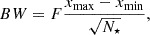
In addition, we included, at the base of the convective envelope, diffusive overshooting (Freytag et al. 1996; Herwig 2000); i.e. an extra-mixing process in which the diffusion coefficient decays exponentially with the distance from the convective boundary defined using the Schwarzschild criterion (located at distance rCE from the stellar centre). Since in MESA the diffusion coefficient in the convective zone goes to zero at rCE, the switch between convection and overshooting is set to occur at r0 = rCE + f0HP, CE, where f0 is a parameter that regulates the diffusion coefficient in the convective envelope at r = r0 and HP, CE is the pressure scale height at the base of the convective envelope. The diffusion coefficient in the overshooting zone is therefore written as
 (1)
(1)
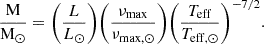
where Dov and D0 are the diffusion coefficients at distance r and r0 from the stellar centre, and fov is the overshooting efficiency. In particular, we set f0 = 0.001 and varied the overshooting efficiency fov from 0.000 to 0.125 (with steps of 0.025), obtaining a grid of 2340 evolutionary tracks (1170 for each value of αMLT).
2.2. Stellar clusters
As mentioned at the beginning of this section, our dataset includes 17 GCs. Since the He content affects the position of the RGBb (see Cassisi & Salaris 1997; Salaris et al. 2006 and Appendix A), we selected GCs with δY2G, 1Gavg ≤ 0.01 and δY2G, 1Gmax ≤ 0.02, where δY2G, 1Gavg and δY2G, 1Gmax are, respectively, the average and the maximum He mass-fraction differences between the second (2G) and the first (1G) generation of stars (see Milone et al. 2018).
We used both Hubble Space Telescope (HST) photometry collected in the HUGS (HST UV Globular cluster Survey; Piotto et al. 2015; Nardiello et al. 2018) catalogue and Gaia EDR3 photometry (Gaia Collaboration 2016, 2023), which is found in the catalogue from Vasiliev & Baumgardt (2021). Both have been corrected for differential reddening, as explained in Sect. 3.2. A probability membership based on proper motions is provided for all sources of each cluster both in the HUGS survey and in the Vasiliev & Baumgardt (2021) catalogue. Consequently, to avoid contamination by field stars, we limited our analysis to stars with a membership probability ≥90%.
The age and [Fe/H] of each GC were taken from Kruijssen et al. (2019) and Carretta et al. (2010), respectively; for the α-element abundance, when a spectroscopic value was not available in Carretta et al. (2010), we used literature values as indicated in Table 1. The only exceptions are NGC 6101, NGC 6144, and NGC 6717, for which we adopted [α/Fe] = 0.4 dex, as suggested in Dotter et al. (2010) and Tailo et al. (2020), since spectroscopic measurements are not available in the literature for these GCs.
Properties (age, chemical composition, and reddening) and RGBb luminosities for all the clusters in our sample.
For the reddening, we used the values from the 3D extinction map by Green et al. (2019) based on Pan-STARRS 1 photometry (Chambers et al. 2016). Because the map is limited to a declination of −30°, for the remaining part of the sky we used extinction values from the Planck Collaboration Int. XLVIII (2016) 2D extinction map. The actual querying of the maps was done with the dustmaps1 Python module (Green 2018).
In order to also explore super-solar metallicities, we included NGC 6791 in the dataset; this is an open cluster for which Gaia DR3 photometry is collected in the catalogue of Hunt & Reffert (2023). For this cluster, we selected stars with a membership probability ≥70% and adopted the age and the reddening reported in Brogaard et al. (2012), while [Fe/H] and [α/Fe] were taken from Brogaard et al. (2011) and Linden et al. (2017), respectively. All the properties of the stellar clusters in our sample are reported in Table 1.
2.3. Field stars
We started from a sample of nearly 104 RGs listed in the catalogue from Willett et al. (2025). This catalogue contains asteroseismic data from Kepler (Borucki et al. 2010; Gilliland et al. 2010), astrometry from Gaia DR3 (Gaia Collaboration 2016, 2023), and spectroscopy from APOGEE DR17 (Majewski et al. 2017; Abdurro’uf et al. 2022). In addition, it includes stellar masses computed from the asteroseismic observables νmax (frequency of maximum oscillation power) and Δν (large frequency separation), using the Bayesian tool PARAM (da Silva et al. 2006; Rodrigues et al. 2014, 2017; Miglio et al. 2021a). The distinction of RGs undergoing shell-hydrogen burning (hence, RGB stars) and core-helium burning (i.e. red clump stars) was done using the flag contained in Yu et al. (2018) based on the distribution of oscillation amplitude, granulation power, and width of power excess.
We restricted the RGB sample to stars with masses lower than 1.5 M⊙ to avoid effects from the convective core overshooting (see e.g. Khan et al. 2018) and from rotational mixing (see e.g. Charbonnel & Lagarde 2010; Lagarde et al. 2012; Beyer & White 2024) during the main sequence (MS) phase. Furthermore, we only selected stars with good astrometric quality (RUWE < 1.4, following prescriptions from Lindegren 2018) and parallaxes with errors up to 10% (according to Gaia DR3) and considered stars with available luminosity derived from the parallaxes corrected for zero-point offset according to the scheme of Lindegren et al. (2021). The final sample is composed of 2737 RGB stars.
3. Methods
A consistent procedure was applied to both simulated and observational data, involving the selection of RGB stars and the computation of a kernel-density estimation (KDE) of their distribution in L and νmax (where available) using the Python package SciPy (Virtanen et al. 2020). Subsequently, the KDE was fitted using a Markov chain Monte Carlo method, which was implemented through the Python package emcee (Foreman-Mackey et al. 2013), to accurately determine the location of the RGBb.
We adopted a fitting function consisting of the superposition of an exponential background and a Gaussian function:
 (2)
(2)
with x being log L (or log νmax), λ the slope of the exponential background (negative for x = log L and positive for x = log νmax), μ and σ the mean and standard deviation of the Gaussian function, and A and B the normalisation factors. We considered all the stars with log L (log νmax) between μ − σ and μ + σ as RGBb stars. An example of the fitting procedure for the GC NGC 1261 is reported in Fig. 1.
 |
Fig. 1. Left panel: HRD of RGB of NGC 1261, with RGBb stars highlighted in orange and by a blue dashed line referring to the RGBb luminosity obtained from the fit. The errors on log LRGBb already include the systematics due to the number of RGB stars (see Appendix B) and the distance modulus (Baumgardt & Hilker 2018). Right panel: KDE (light blue zone) of luminosity distribution (lower labels) and relative fit (orange line). The blue line represents the histogram of the RGB luminosity with Poissonian errors (upper labels). |
Finally, for both the field stars and stellar clusters, we inferred the overshooting efficiency by comparing our observational and theoretical results. In the following sections, we describe these procedures for the evolutionary tracks and the two observational datasets in detail.
3.1. Simulated data
In the case of evolutionary tracks, RGB stars were defined as points cooler than the MS turn-off and having a surface gravity lower than a threshold value (in order to avoid the sub-giant branch). After the selection of the RGB, we generated a synthetic population for each track extracting 5000 stars that are uniformly distributed in age, and we computed the luminosity (log L), the effective temperature (Teff), and the frequency of maximum oscillation power (νmax) through interpolation, adding normally distributed deviations to these three quantities to simulate photometric errors on magnitudes and colours. After that we computed the KDE both for log L and log νmax, and fitted it with Eq. (2). The fitting of simulations was also used to test the script and compute the systematics on the estimated RGBb location due to the number of stars in the fitted sample, as described in Appendix B.
3.2. Analysis of stellar clusters
For each GC, before fitting the RGB luminosity distribution and determining the overshooting efficiency, we determined the average mass of stars on the RGB and de-reddened the data in order to compute the effective temperature and the luminosity of each star. All these procedures are described in detail in the following paragraphs.
We derived a mass–age–metallicity scaling relation from the models, which we used to infer the average stellar mass at the RGBb (MRGBb) for each cluster, given the age and the chemical composition:
![Mathematical equation: $$ \begin{aligned} \biggl (\frac{\mathrm{M} _\mathrm{RGBb} }{\mathrm{M} _\odot }\biggr ) = A\biggl (\frac{t_\mathrm{Age} }{10^9\; \mathrm{yr}}\biggr )^\alpha + B[\mathrm{M}/\mathrm{H}]^\beta , \end{aligned} $$](/articles/aa/full_html/2025/08/aa53980-25/aa53980-25-eq21.gif) (3)
(3)
with A = 1.906 ± 0.003, α = ( − 2.671 ± 0.003)⋅10−1, B = (1.551 ± 0.007)⋅10−1, and β = (5.665 ± 0.013)⋅10−1. This scaling relation has been computed at the RGBb luminosity for each model. The coefficients A, α, B, and β show very little variation with the overshooting efficiency (see Appendix C); hence, we decided to work with the median value of each parameter.
In order to perform the fit on the best possible data, after the membership selection, we corrected the HST and Gaia photometry of sixteen and seven GCs, respectively, for the effects of differential reddening following the method described in Milone et al. (2012). To do so, we focused our attention on RGB stars to define the reference sample. Even though they are less numerous, we prefer RGBs to MS stars since their photometric error is lower. For each star in the target GCs, the differential reddening value, ΔE(B − V), was computed as the median offset from the RGB mean ridge line, defined in a colour–magnitude diagram (CMD) tilted along the reddening vector, among the 30–60 closest reference stars. We assumed the Cardelli et al. (1989) extinction law, adopting RV = 3.1. This iterative procedure was repeated for each star until the residual on the ΔE(B − V) matched the photometric error. Typically, we reach convergence after two iterations. In Figure 2, we show an example of the differential reddening on the CMD of NGC 6144, while in Figure 3 we plot the reddening map we derived.
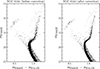 |
Fig. 2. Comparison between CMDs of NGC 6144 before (left panel) and after (right panel) applying differential reddening correction. |
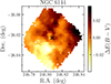 |
Fig. 3. Differential reddening map for GC NGC 6144 obtained using HST data sampling radial range up to ∼1.0 half-light radius2. The black cross marks the centre of the cluster (Vasiliev & Baumgardt 2021). |
After the de-reddening procedure, we converted colours and magnitudes into effective temperatures and luminosities, respectively. This was done using the bolometric corrections (BCs) from Casagrande & VandenBerg (2014), the distances from the 2023 version of the Baumgardt & Hilker (2018) catalogue, and the reddenings reported in Table 1.
For each GC, we built a synthetic grid of stars with different values of surface gravity and effective temperature (0.2 ≤ log g ≤ 5.5, with steps of 0.1; 3000 K ≤ Teff ≤ 8000 K, with steps of 5 K) and computed the BCs in the F606W and F814W bands for each point. We then inferred log g for each star from the isochrone relative to the cluster and assigned the temperature in the grid corresponding to the value of BCF814W − BCF606W closest to the real colour of the star. We compared our evolutionary tracks with the corresponding ones from the PARSEC database (Bressan et al. 2012; Chen et al. 2014, 2015; Fu et al. 2018). Given the small difference in log g at fixed luminosity (⟨Δlog gMESA − PARSEC⟩∼ − 0.02), we decided to use PARSEC isochrones instead of computing our own.
After obtaining the Hertzsprung-Russell diagram (HRD) for each cluster, we used TOPCAT (Tool for OPerations on Catalogs And Tables; Taylor 2005) to properly separate the RGB from the horizontal branch and the asymptotic giant branch, and fitted the KDE of the luminosity distribution with Eq. (2). We performed the fit for luminosities greater than the one corresponding to the KDE maximum, since the cut at the base of the RGB affects the counts in the lowest luminosity bins and, hence, the slope of the exponential background. We excluded NGC 5053 and NGC 6535 because their RGBs contain too few stars to make a robust prediction on the RGBb position (see App. B). The HRDs of seven out of 17 GCs were completed by adding stars from the Vasiliev & Baumgardt (2021) catalogue containing Gaia DR3 photometry (Gaia Collaboration 2016, 2023); for these stars, we used the colour-temperature relation from Mucciarelli et al. (2021) and the BCs from Andrae et al. (2018).
Once the luminosity of the RGBb was determined, we restricted our sample to clusters with at least ten RGBb stars (ending up with 11 GCs out of 17), and we performed an interpolation in the M − log L − [M/H]−fov space to derive the overshooting efficiency for each GC. This operation was repeated 104 times, randomly extracting a pair ([M/H], log L) from a normal distribution centred on the expected values of the two quantities and with σs corresponding to the associated errors. An example is provided in Fig. 4.
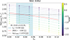 |
Fig. 4. Representation in fov − log L plane of interpolation procedure to derive overshooting efficiency for GC NGC 6362. The expectation values of [M/H] and log LRGBb are represented by the solid red line and the dashed black one, respectively, and are plotted on the grid of models computed at the cluster mass (coloured according to metallicity). The light blue shaded zone represents the confidence interval at 68% of the derived overshooting efficiency. |
For the OC NGC 6791, the methods were the same, except for the de-reddening procedure, which we did not perform due to a low number of stars along the RGB, and the conversion of HST colours and magnitudes into temperatures and luminosities, since for this cluster we only used Gaia photometry. Furthermore, for this cluster we used the distance modulus reported in Brogaard et al. (2011).
3.3. Analysis of field stars
We divided our 2737 RGB stars into bins of different masses ([0.7, 0.9[, [0.9, 1.1[, [1.1, 1.3[, [1.3, 1.5[, in solar masses) and metallicities ([−0.8, −0.6[, [−0.6, −0.4[, [-0.4, −0.2[, [−0.2, +0.0[, [+0.0, +0.2[, [+0.2, +0.4[ dex). We only considered bins with at least 60 stars, ending up with 1924 stars arranged in 11 bins (see Tab. 2).
Properties and RGBb locations for the bins of field stars in our sample.
Unlike what we did for synthetic populations and stellar clusters, for each bin, we only fitted the highest peak with a Gaussian function – both in the log L axis and log νmax axis – since the exponential background was not well identifiable in all the combinations of mass and metallicity bins. After that, we performed an interpolation in the M − log L (log νmax)−[M/H]−fov space to derive the overshooting efficiency for each bin, in the same way we did for stellar clusters (see Sect. 3.2).
4. Results and discussion
In this section, we present our results on the determination of the RGBb locations and the overshooting efficiencies, adding a comparison between the bumps determined from luminosity and νmax, as well as a comment on the effects of changing αMLT. Finally, we discuss a possible interpretation of the correlation between the overshooting efficiency and the metallicity.
4.1. RGBb location
We derived the variations of the RGBb location in luminosity and in νmax from the grid of models in response to changes in stellar parameters (i.e. mass, metallicity, overshooting efficiency) and compared them to those emerging from the analysis of GCs and field stars. Specifically, we observed from the evolutionary tracks that νmax, RGBb decreases with increasing stellar mass and decreasing metallicity, while the RGBb luminosity exhibits opposite trends (as already discussed by, e.g., Fusi Pecci et al. 1990; Cassisi & Salaris 1997; Riello et al. 2003; Di Cecco et al. 2010; Nataf et al. 2013, and Khan et al. 2018). This phenomenon can be attributed to the fact that, in the range of masses explored, more massive stars – as well as those with lower metallicity – are hotter and consequently have a shallower convective envelope and a more luminous RGBb. Thus, since an increase in luminosity along the RGB corresponds to an increase in radius (R), and given that νmax is strongly dependent on R (νmax ∝ MR−2Teff−1/2; see e.g. Brown et al. 1991; Kjeldsen & Bedding 1995; Belkacem et al. 2011), we expect νmax, RGBb to exhibit trends opposing those observed for luminosity. In addition, we found lower RGBb luminosities (or, equivalently, higher νmax, RGBb values) for higher values of the overshooting efficiency; this is due to the fact that a more efficient overshooting produces a deeper mixing zone, leading to a less luminous RGBb.
We inferred the RGBb luminosities for stellar clusters (see Tab. 1 and Fig. 5) and the RGBb location in L and νmax for field stars (see Tab. 2, Fig. 6 and Fig. 7), obtaining trends with masses and metallicities that broadly reflect the expectations from models. For the OC NGC 6791, we were also able to estimate the RGBb νmax, given that some giants belonging to that cluster, including four RGBb stars, have been observed by Kepler and were included in our sample from the catalogue of Willett et al. 2025 (see Fig. 8). Computing the νmax median value of those four stars, we obtained  .
.
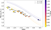 |
Fig. 5. RGBb luminosity as function of [M/H] for stellar clusters in our sample (coloured according to MRGBb). The RGBb luminosity decreases with increasing [M/H] and decreasing stellar mass (see e.g. NGC 1261 and NGC 6218). The lines correspond to the RGBb luminosities – at different metallicities – of evolutionary tracks with M = (0.8, 1.17) M⊙ (orange, blue) and fov = 0.000, 0.025 (dotted, dashed). |
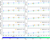 |
Fig. 6. Location of RGBb in log νmax (left) and log L (right) as function of stellar mass, for Kepler stars divided in metallicity bins (orange points). The points coloured from green to blue represent the location of the RGBb in the same metallicity bins for different overshooting efficiencies. The colour-coding for fov is reported in the bottom horizontal bar. |
Our results are also consistent with previous studies. In particular, we compared our RGBb positions in GCs with the ones presented in Nataf et al. 2013 (which we converted from V magnitude to log L with the bolometric corrections from Casagrande & VandenBerg 2014). Despite a little systematic offset between the two works (the median difference between log LNataf and log Lthis work is  ), we found general agreement, as shown in Fig. 9. We also found that the RGBb frequencies of our field stars are compatible with the ones obtained by Khan et al. 2018 (see Fig. 7).
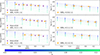 |
Fig. 7. Location of RGBb in log νmax (left) and log L (right) as function of metallicity, for Kepler stars divided in mass bins (orange points). The points coloured from green to blue represent the location of the RGBb in the same mass bins for different overshooting efficiencies. The colour-coding for fov is reported in the bottom horizontal bar. Our data are plotted as orange dots, while the results from Khan et al. 2018 are reported as purple stars (left panels). |
4.2. Comparison between LRGBb and νmax, RGBb
As mentioned above, we derived the RGBb location with two different observables: luminosity and frequency of maximum oscillation power. This allowed us to obtain two more measurements of log LRGBb to compare with the one coming from the fit (log Lfit).
The first additional measurement (log Lνmax) comes from the median luminosity of the stars that were selected as RGBb stars according to their νmax (as explained in Sect. 3). In all the bins of field stars, log Lfit and log Lνmax are compatible, meaning that the fits in log L and log νmax classify almost the same objects as RGBb stars (see Table 3). The second additional measurement (log Lscaling) was derived from the asteroseismic scaling relations (see e.g. Brown et al. 1991; Frandsen et al. 2007; Chaplin & Miglio 2013; Miglio et al. 2016, 2021a) and, in particular, from the one that combines M, L, νmax, and Teff:
 (4)
(4)
Comparison between three different measurements of log LRGBb for field stars.
Also in this case, we found agreement with log Lfit, with the exception of the bin with M/M⊙ ∈ [1.3, 1.5[ and [M/H]∈[−0.4, −0.2[ dex, for which the luminosity computed with Eq. (4) is higher (see Table 3).
This bin presents, compared with the others, an anomalously low RGBb luminosity (see Figs. 6 and 7), and the evolution of its stars could be affected by effects such as core overshooting (Khan et al. 2018) and rotation (Charbonnel & Lagarde 2010; Lagarde et al. 2012; Beyer & White 2024) during the MS, which start to arise in these intervals of mass and metallicity. We thus decided to exclude this bin from our analysis.
4.3. Effects of changing the mixing-length parameter
As mentioned in Sect. 2.1, we computed our grid of evolutionary tracks with two different values of αMLT, which is the parameter that regulates the length of the mean free path and the size of the convective cells according to the MLT (Böhm-Vitense 1958). The values we chose are (i) αMLT = 2.290, which comes from the solar calibration of our models; and (ii) αMLT = 2.090, which gives a better fit to the temperatures from APOGEE, as explained below.
Variations of this parameter affect stellar radii and effective temperatures. Specifically, an increment of αMLT produces stellar models with higher temperatures and smaller radii (Cox & Giuli 1968). This implies variations in νmax and, to a lesser extent, in luminosities (since the increment in effective temperature and the decrement in radius tend to compensate each other). Since a modification of αMLT produces different variations of the RGBb location in L and νmax, we also expect to find different overshooting efficiencies for different values of αMLT, with different impacts on fovL and fovνmax. In this work, we found the best agreement between fovL and fovνmax for αMLT = 2.090 (see Sect. 4.4).
Crucially, we found that this value of αMLT also significantly improves the agreement between the predicted and observed Teff. Specifically, we computed the median ΔTeff = Teff, data − Teff, track for each bin of field stars (an example is reported in Fig. 10), finding that the tracks with αMLT = 2.090 adapt better to the data in all our bins. In addition, we computed the median of all those quantities, finding  for αMLT = 2.090 and
  for αMLT = 2.290. A similar conclusion is reached for the OC NGC 6791, as shown in Fig. 8.
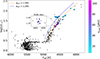 |
Fig. 8. HRD of NGC 6791, with stars observed by Kepler coloured according to νmax. The inset zoomed-in views show the RGBb stars, including the four stars for which we have νmax values from Kepler. The orange and blue lines correspond to the evolutionary tracks with αMLT = 2.090 and αMLT = 2.290, respectively, and no envelope overshooting. |
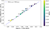 |
Fig. 9. Comparison between our RGBb luminosities and those presented in Nataf et al. (2013). |
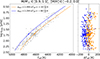 |
Fig. 10. Left panel: Teff − log νmax diagram for field stars with M/M⊙ ∈ [0.9, 1.1[ and [M/H]∈[−0.2, 0.0[ dex (grey points) and corresponding evolutionary tracks with αMLT = 2.090 (orange line) and αMLT = 2.290 (blue line). Right panel: Temperature differences between data and evolutionary tracks, with the same colour-coding of the left panel. |
4.4. Envelope overshooting calibration
As already mentioned in Sect. 3, after deriving the RGBb luminosities and νmax, we performed an interpolation to infer the overshooting efficiencies for both stellar clusters and field stars in order to look for a correlation with [M/H]. We obtained overshooting efficiencies, fov, spanning from  to 0.064−0.016+0.015 and, in particular, not greater than
  for field stars (see Table 4). This result is consistent with the constraints presented in Khan et al. (2018), where an upper limit of ∼0.05 for fov in field stars with M/M⊙ ∈ [0.9, 1.5] and [M/H]∈[−0.5, +0.3] dex is found.
Interpolation results.
Regarding the correlation between fov and [M/H], we first computed the Spearman correlation index (ρS; see Spearman 1904), which measures the rank of correlation between two variables. We found ρS, 2.090 = −0.718 and ρS, 2.290 = −0.607, both with p values lower than 1%, indicating an anti-correlation between fov and [M/H]. We consequently tried to fit the points with a linear relation of the kind fov = m ⋅ [M/H]+q, finding a negative slope in all cases we analysed (see Tab. 5).
Results of the fits on the fov − [M/H] plane, each one with the corresponding αMLT value and metallicity range.
This process was repeated for both values of αMLT (2.090, 2.290). Although we consider the results obtained from the interpolation along the grid with αMLT = 2.090 to be more reliable, as we fitted the effective temperatures (see Sect. 4.3) we also present the results obtained with αMLT = 2.290. The behaviour of the relation is similar in both cases, indicating that our conclusions are robust and not significantly affected by this systematic effect.
Starting from the overshooting efficiency derived from the bump luminosity (fovL), which has been computed for [M/H] between −2.02 dex and +0.35 dex, we found a relation with a weakly negative slope that is steeper for αMLT = 2.090 (see Fig. 11 and Tab. 5). We performed a t-Student test (Student 1908; Fornasini 2008) on our fit results, using the Python package statsmodels (Skipper & Josef 2010). We found in both cases that the p value is lower than 1%, meaning that the slope is significant and that we can reject the hypothesis of a flat relation.
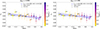 |
Fig. 11. Overshooting efficiency derived from LRGBb as function of [M/H], both for αMLT = 2.090 (left panel) and αMLT = 2.290 (right panel). Clusters are represented as circles, while field stars are shown as triangles. The blue lines correspond to the linear fits. Points are coloured by stellar mass. |
For the overshooting efficiency derived from νmax, RGBb (fovνmax, obtained for field stars and the OC NGC 6791, for [M/H] between −0.5 dex and +0.35 dex), we found the same slope for the two different values of αMLT, steeper than the one related to fovL (see Fig. 12 and Tab. 5). In both cases, αMLT = 2.090 and αMLT = 2.290, fovL, and fovνmax are compatible within 1σ (see Table 4), and, if we only consider the metallicity range where we measured both the different fov ([M/H]∈[−0.5, +0.35] dex), we find that fovL and fovνmax are related to [M/H] with the same slope, meaning that extending the metallicity range with the inclusion of GCs implies a flattening of the relation. In addition, we observe that when the interpolation is performed along the grid with αMLT = 2.090, the shift in fov between the two relations is smaller (see Fig. 13 and Tab. 5).
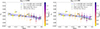 |
Fig. 12. Same as Fig. 11, but with the addition of the overshooting efficiencies derived from νmax, RGBb (open symbols) and the relative fits (green lines). |
The flattening of the relation at low metallicities led us to consider the possibility of fitting our data with a broken-line function. To see whether this model adapts to our data better than the single straight line, we performed the t-Student test again using the Python library piecewise-regression (Pilgrim 2021), and we found that the hypothesis of no breakpoints cannot be rejected and that the relation with no breakpoints (i.e. the straight line) is the preferable one.
To investigate the primary contributors to the current uncertainty in the inferred overshooting efficiency, we used the GC NGC 6362 as a case study. This cluster has intermediate metallicity ([M/H]= − 0.80 ± 0.11), which lies within the [M/H] range of our sample. We applied variations of the order of their typical observational uncertainties to several parameters: Teff by ±100 K, [M/H] by ±0.05 dex, age by ±0.5 Gyr, and distance modulus by ±0.03. For each variation, we computed the effects on the inferred log g, the bolometric corrections (BCs), and, consequently, the RGBb luminosity of the cluster. We then interpolated along the model grid using the new values of age (tAge), metallicity ([M/H]), and log LRGBb to compute the associated variations in fov. Our results show that metallicity is the dominant contributor to the variation in fov, accounting for approximately 19%, followed by Teff and distance modulus (each contributing about 11%), and age (tAge), which contributes around 8%. On the other hand, Teff and the distance modulus have a greater impact on the RGBb luminosity than [M/H] and tAge (see Fig. 14). These findings indicate that to improve the precision of the overshooting efficiency measurements, a more accurate determination of metallicity is crucial, along with better constraints on temperature and distance.
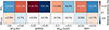 |
Fig. 14. Relative variations of RGBb luminosity and overshooting efficiency for the GC NGC 6362 produced by variations of effective temperature (Teff), metallicity ([M/H]), age (tAge), and distance modulus (dm). |
4.5. A possible interpretation
Given the anti-correlation between overshooting efficiency and metallicity (see Sect. 4.4), we investigated, as was done in Khan 2021, possible correlations of [M/H] with the Brunt-Väisälä frequency, the characteristic frequency of internal gravity waves (i.e. oscillations driven by buoyancy), defined as
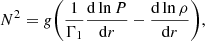 (5)
(5)
where g is the gravitational acceleration, Γ1 = (∂lnP/∂lnρ)ad is one of the three adiabatic exponents, and P and ρ are pressure and density, respectively. Assuming the ideal gas law for a fully ionised gas, the square of the Brunt-Väisälä frequency can also be expressed in terms of the adiabatic (∇ad = (∂lnT/∂lnP)ad) and radiative (∇rad = dlnT/dlnP) temperature gradients, and the mean molecular weight gradient (∇μ = dlnμ/dlnP), with the following approximation:
 (6)
(6)
which shows that N2 is negative in convective zones and positive in radiative zones. From our models, we observe that the profile of the squared Brunt-Väisälä frequency near the convective border is steeper at higher metallicities (see Fig. 15).
 |
Fig. 15. Profiles of squared Brunt-Väisälä frequency, N2, for models with M = 1 M⊙ and [M/H]= − 0.5, −0.3, −0.1, +0.1, +0.3 dex. The x-axis is normalised by the position rCE of the convective border, indicated by the vertical dashed black line |
This has implications on the bulk Richardson number, RiB (Lettau & Davidson 1957), a quantification of the stiffness of the convective boundary: low values (∼10) of RiB allow convective boundary mixing, while high values (∼104) are associated with a stiff boundary that inhibits convective boundary mixing (Cristini et al. 2016). Mathematically, RiB corresponds to the ratio between the potential energy of restoration of the convective boundary and the kinetic energy of turbulent eddies:
 (7)
(7)
where ℒ is a length scale associated with the turbulent motion, while ΔB is the buoyancy jump over a distance 2Δr from the boundary position rB:
 (8)
(8)
From the last two equations, we can deduce that steeper profiles of N2 produce higher buoyancy jumps and, consequently, higher values of RiB; hence, steeper convective boundaries occur. An analogous connection between RiB (hence, the profile of N2) and the extension of the mixing zone is found in Meakin & Arnett 2007, which states that the entrainment coefficient, E –i.e. the ratio between the time rate of change of the boundary position through turbulent entrainment (Kantha et al. 1977; Strang & Fernando 2001), ve, and the rms turbulent velocity of the fluid elements, vc– is inversely proportional to a power of the bulk Richardson number:
 (9)
(9)
Typical values of A and n are in the ranges [0.1; 0.5] and [1.00; 1.75], respectively (Meakin & Arnett 2007).
We can thus suppose that the decrease of the overshooting efficiency with increasing metallicity could be associated with the steepening of the squared Brunt-Väisälä profile below the convective zone.
5. Summary and conclusions
In this work, we extended the study described in Khan et al. (2018), with the aim of calibrating the efficiency of convective-envelope overshooting in RGB stars.
First, we derived the RGBb location in log νmax and log L for the widest mass and metallicity domain explored to date, including both stellar clusters and field stars. We found that the RGBb luminosity decreases with increasing metallicity and decreasing mass, and, contextually, the RGBb νmax follows the opposite trends (see Sect. 4.1), confirming results from previous works (Nataf et al. 2013; Khan et al. 2018).
After that, from the comparison between the RGBb locations in our datasets and in our grid of evolutionary tracks, we derived overshooting efficiencies (fov, i.e. the rate, in units of HP, at which the diffusion coefficient decays exponentially getting further from the convective envelope; see Sect. 2.1) for stellar clusters and field stars and studied a correlation of this quantity with metallicity, measuring overshooting efficiencies ranging from  to 0.062−0.015+0.017. We found that fov decreases with increasing metallicity and that the most suitable model to describe this trend in our data is a linear relation with slope ( − 0.010 ± 0.006) dex−1 (see Sect. 4.4), which is significant according to the t-Student test (Student 1908; Fornasini 2008). We then explored the behaviour of the Brunt-Väisälä frequency under [M/H] variations, finding that at higher metallicities N2 presents steeper profiles, increasing the buoyancy jump and, consequently, limiting the extension of the mixed zone (see Sec. 4.5). This means that our correlation could be compatible with expectations from recent works concerning entrainment (Meakin & Arnett 2007).
We investigated the main contributors to the overshooting efficiency uncertainty, and we found that the overshooting efficiency is mainly affected by [M/H] and, secondarily, by the measurements of effective temperatures and distance moduli (see Sect. 4.4). On the other hand, we found that our results are not significantly affected by variations of the mixing-length parameter (see Sect. 4.3) or by the choice of the helium-to-metals enrichment ratio (see App. A).
A further step in this work would be to compare our findings to predictions from 3D hydrodynamical simulations (Blouin et al. 2023) and try to define the overshooting efficiency as a function of metallicity, in order to reduce the number of free parameters in stellar models. Finally, in addition to the indirect tests of envelope mixing presented here, high-precision asteroseismic observations across a broad range of globular clusters (GCs), such as those proposed by the candidate space mission HAYDN (Miglio et al. 2021b), would provide more detailed localised inferences on the properties of convective envelopes and mixing through the study of individual oscillation modes (Lindsay et al. 2022). This would offer valuable empirical insights into the physical nature of convective boundary mixing.
Acknowledgments
L.B. aknowledges financial support from MUR (Ministero dell’Universitáe della Ricerca) and NextGenerationEU throughout the PNRR ex D.M. 118/2023. L.B. acknowledges Nadège Lagarde, Lorenzo Martinelli, David Nataf and Walter van Rossem for their useful suggestions. M.T., A.Miglio, and M.M. acknowledge support from the ERC Consolidator Grant funding scheme (project ASTEROCHRONOMETRY, G.A. n. 772293 http://www.asterochronometry.eu). A.Mazzi acknowledges financial support from Bologna University, “MUR FARE Grant Duets CUP J33C21000410001”. A.Mucciarelli acknowledges support from the project “LEGO – Reconstructing the building blocks of the Galaxy by chemical tagging” (P.I. A. Mucciarelli). granted by the Italian MUR through contract PRIN 2022LLP8TK_001. S.K. is funded by the Swiss National Science Foundation through an Eccellenza Professorial Fellowship (award PCEFP2_194638). We thank the anonymous referee for the helpful comments which helped us improve the paper.
References
- Abdurro’uf, Accetta, K., Aerts, C., et al. 2022, ApJS, 259, 35 [NASA ADS] [CrossRef] [Google Scholar]
- Alongi, M., Bertelli, G., Bressan, A., & Chiosi, C. 1991, A&A, 244, 95 [NASA ADS] [Google Scholar]
- Andrae, R., Fouesneau, M., Creevey, O., et al. 2018, A&A, 616, A8 [NASA ADS] [CrossRef] [EDP Sciences] [Google Scholar]
- Baraffe, I., Pratt, J., Goffrey, T., et al. 2017, ApJ, 845, L6 [Google Scholar]
- Baraffe, I., Pratt, J., Vlaykov, D. G., et al. 2021, A&A, 654, A126 [NASA ADS] [CrossRef] [EDP Sciences] [Google Scholar]
- Baraffe, I., Constantino, T., Clarke, J., et al. 2022, A&A, 659, A53 [NASA ADS] [CrossRef] [EDP Sciences] [Google Scholar]
- Baumgardt, H., & Hilker, M. 2018, MNRAS, 478, 1520 [Google Scholar]
- Belkacem, K., Goupil, M. J., Dupret, M. A., et al. 2011, A&A, 530, A142 [CrossRef] [EDP Sciences] [Google Scholar]
- Beyer, A. C., & White, R. J. 2024, ApJ, 973, 28 [Google Scholar]
- Blouin, S., Mao, H., Herwig, F., et al. 2023, MNRAS, 522, 1706 [CrossRef] [Google Scholar]
- Böhm-Vitense, E. 1958, Z. Astrophys., 46, 108 [Google Scholar]
- Borucki, W. J., Koch, D., Basri, G., et al. 2010, Science, 327, 977 [Google Scholar]
- Bragaglia, A., Carretta, E., D’Orazi, V., et al. 2017, A&A, 607, A44 [NASA ADS] [CrossRef] [EDP Sciences] [Google Scholar]
- Bressan, A., Bertelli, G., & Chiosi, C. 1986, Mem. Soc. Astron. It., 57, 411 [NASA ADS] [Google Scholar]
- Bressan, A. G., Chiosi, C., & Bertelli, G. 1981, A&A, 102, 25 [Google Scholar]
- Bressan, A., Marigo, P., Girardi, L., et al. 2012, MNRAS, 427, 127 [NASA ADS] [CrossRef] [Google Scholar]
- Brogaard, K., Bruntt, H., Grundahl, F., et al. 2011, A&A, 525, A2 [NASA ADS] [CrossRef] [EDP Sciences] [Google Scholar]
- Brogaard, K., VandenBerg, D. A., Bruntt, H., et al. 2012, A&A, 543, A106 [NASA ADS] [CrossRef] [EDP Sciences] [Google Scholar]
- Brown, T. M., Gilliland, R. L., Noyes, R. W., & Ramsey, L. W. 1991, ApJ, 368, 599 [Google Scholar]
- Buldgen, G., Noels, A., Amarsi, A. M., et al. 2025, A&A, 694, A285 [NASA ADS] [CrossRef] [EDP Sciences] [Google Scholar]
- Cardelli, J. A., Clayton, G. C., & Mathis, J. S. 1989, ApJ, 345, 245 [Google Scholar]
- Carretta, E., Bragaglia, A., Gratton, R. G., et al. 2010, A&A, 516, A55 [NASA ADS] [CrossRef] [EDP Sciences] [Google Scholar]
- Casagrande, L., & VandenBerg, D. A. 2014, MNRAS, 444, 392 [Google Scholar]
- Cassisi, S., & Salaris, M. 1997, MNRAS, 285, 593 [NASA ADS] [Google Scholar]
- Chambers, K. C., Magnier, E. A., Metcalfe, N., et al. 2016, ArXiv e-prints [arXiv:1612.05560] [Google Scholar]
- Chaplin, W. J., & Miglio, A. 2013, ARA&A, 51, 353 [Google Scholar]
- Charbonnel, C., & Lagarde, N. 2010, A&A, 522, A10 [CrossRef] [EDP Sciences] [Google Scholar]
- Chen, Y., Girardi, L., Bressan, A., et al. 2014, MNRAS, 444, 2525 [Google Scholar]
- Chen, Y., Bressan, A., Girardi, L., et al. 2015, MNRAS, 452, 1068 [Google Scholar]
- Christensen-Dalsgaard, J., Monteiro, M. J. P. F. G., Rempel, M., & Thompson, M. J. 2011, MNRAS, 414, 1158 [CrossRef] [Google Scholar]
- Cox, J. P., & Giuli, R. T. 1968, Principles of Stellar Structure (New York: Gordon and Breach) [Google Scholar]
- Cristini, A., Meakin, C., Hirschi, R., et al. 2016, Phys. Scr., 91, 034006 [Google Scholar]
- da Silva, L., Girardi, L., Pasquini, L., et al. 2006, A&A, 458, 609 [NASA ADS] [CrossRef] [EDP Sciences] [Google Scholar]
- Di Cecco, A., Bono, G., Stetson, P. B., et al. 2010, ApJ, 712, 527 [Google Scholar]
- Dotter, A., Sarajedini, A., Anderson, J., et al. 2010, ApJ, 708, 698 [Google Scholar]
- Fagotto, F., Bressan, A., Bertelli, G., & Chiosi, C. 1994, A&AS, 104, 365 [NASA ADS] [Google Scholar]
- Foreman-Mackey, D., Hogg, D. W., Lang, D., & Goodman, J. 2013, PASP, 125, 306 [Google Scholar]
- Fornasini, P. 2008, The Uncertainty in Physical Measurements (New York: Springer) [Google Scholar]
- Frandsen, S., Bruntt, H., Grundahl, F., et al. 2007, A&A, 475, 991 [NASA ADS] [CrossRef] [EDP Sciences] [Google Scholar]
- Freytag, B., Ludwig, H. G., & Steffen, M. 1996, A&A, 313, 497 [NASA ADS] [Google Scholar]
- Fu, X., Bressan, A., Marigo, P., et al. 2018, MNRAS, 476, 496 [NASA ADS] [CrossRef] [Google Scholar]
- Fusi Pecci, F., Ferraro, F. R., Crocker, D. A., Rood, R. T., & Buonanno, R. 1990, A&A, 238, 95 [NASA ADS] [Google Scholar]
- Gaia Collaboration (Prusti, T., et al.) 2016, A&A, 595, A1 [NASA ADS] [CrossRef] [EDP Sciences] [Google Scholar]
- Gaia Collaboration (Vallenari, A., et al.) 2023, A&A, 674, A1 [NASA ADS] [CrossRef] [EDP Sciences] [Google Scholar]
- Gilliland, R. L., Brown, T. M., Christensen-Dalsgaard, J., et al. 2010, PASP, 122, 131 [Google Scholar]
- Green, G. 2018, J. Open Source Softw., 3, 695 [NASA ADS] [CrossRef] [Google Scholar]
- Green, G. M., Schlafly, E., Zucker, C., Speagle, J. S., & Finkbeiner, D. 2019, ApJ, 887, 93 [NASA ADS] [CrossRef] [Google Scholar]
- Hasselquist, S., Holtzman, J. A., Shetrone, M., et al. 2019, ApJ, 871, 181 [NASA ADS] [CrossRef] [Google Scholar]
- Herwig, F. 2000, A&A, 360, 952 [NASA ADS] [Google Scholar]
- Hunt, E. L., & Reffert, S. 2023, A&A, 673, A114 [NASA ADS] [CrossRef] [EDP Sciences] [Google Scholar]
- Iben, I. 1968, Nature, 220, 143 [NASA ADS] [CrossRef] [Google Scholar]
- Jofré, P. 2021, ApJ, 920, 23 [CrossRef] [Google Scholar]
- Joyce, M., & Chaboyer, B. 2015, ApJ, 814, 142 [Google Scholar]
- Kantha, L. H., Phillips, O. M., & Azad, R. S. 1977, J. Fluid Mech., 79, 753 [Google Scholar]
- Khan, S. 2021, PhD thesis, School of Physics and Astronomy, University of Birmingham, United Kingdom [Google Scholar]
- Khan, S., Hall, O. J., Miglio, A., et al. 2018, ApJ, 859, 156 [NASA ADS] [CrossRef] [Google Scholar]
- King, C. R., Da Costa, G. S., & Demarque, P. 1985, ApJ, 299, 674 [NASA ADS] [CrossRef] [Google Scholar]
- Kjeldsen, H., & Bedding, T. R. 1995, A&A, 293, 87 [NASA ADS] [Google Scholar]
- Komatsu, E., Smith, K. M., Dunkley, J., et al. 2011, ApJS, 192, 18 [Google Scholar]
- Krishna Swamy, K. S. 1966, ApJ, 145, 174 [Google Scholar]
- Kruijssen, J. M. D., Pfeffer, J. L., Reina-Campos, M., Crain, R. A., & Bastian, N. 2019, MNRAS, 486, 3180 [Google Scholar]
- Lagarde, N., Decressin, T., Charbonnel, C., et al. 2012, A&A, 543, A108 [NASA ADS] [CrossRef] [EDP Sciences] [Google Scholar]
- Lettau, H., & Davidson, B. 1957, Exploring the Atmosphere’sFirst Mile: Proceedings of the Great Plains Turbulence Field Program, 1 August to 8 September 1953 (Symposium Publications Division, Pergamon Press) [Google Scholar]
- Lindegren, L. 2018, GAIA-C3-TN-LU-LL-124-01 [Google Scholar]
- Linden, S. T., Pryal, M., Hayes, C. R., et al. 2017, ApJ, 842, 49 [NASA ADS] [CrossRef] [Google Scholar]
- Lindegren, L., Bastian, U., Biermann, M., et al. 2021, A&A, 649, A4 [EDP Sciences] [Google Scholar]
- Lindsay, C. J., Ong, J. M. J., & Basu, S. 2022, ApJ, 931, 116 [CrossRef] [Google Scholar]
- Maeder, A. 1975, A&A, 40, 303 [NASA ADS] [Google Scholar]
- Majewski, S. R., Schiavon, R. P., Frinchaboy, P. M., et al. 2017, AJ, 154, 94 [NASA ADS] [CrossRef] [Google Scholar]
- Marino, A. F., Milone, A. P., Renzini, A., et al. 2021, ApJ, 923, 22 [CrossRef] [Google Scholar]
- Massari, D., Mucciarelli, A., Dalessandro, E., et al. 2017, MNRAS, 468, 1249 [Google Scholar]
- Meakin, C. A., & Arnett, D. 2007, ApJ, 667, 448 [NASA ADS] [CrossRef] [Google Scholar]
- Miglio, A., Chaplin, W. J., Brogaard, K., et al. 2016, MNRAS, 461, 760 [NASA ADS] [CrossRef] [Google Scholar]
- Miglio, A., Chiappini, C., Mackereth, J. T., et al. 2021a, A&A, 645, A85 [NASA ADS] [CrossRef] [EDP Sciences] [Google Scholar]
- Miglio, A., Girardi, L., Grundahl, F., et al. 2021b, Exp. Astron., 51, 963 [NASA ADS] [CrossRef] [Google Scholar]
- Milone, A. P., Piotto, G., Bedin, L. R., et al. 2012, A&A, 540, A16 [NASA ADS] [CrossRef] [EDP Sciences] [Google Scholar]
- Milone, A. P., Marino, A. F., Renzini, A., et al. 2018, MNRAS, 481, 5098 [NASA ADS] [CrossRef] [Google Scholar]
- Mucciarelli, A., Bellazzini, M., & Massari, D. 2021, A&A, 653, A90 [NASA ADS] [CrossRef] [EDP Sciences] [Google Scholar]
- Nardiello, D., Libralato, M., Piotto, G., et al. 2018, MNRAS, 481, 3382 [NASA ADS] [CrossRef] [Google Scholar]
- Nataf, D. M., Gould, A. P., Pinsonneault, M. H., & Udalski, A. 2013, ApJ, 766, 77 [NASA ADS] [CrossRef] [Google Scholar]
- O’Malley, E. M., & Chaboyer, B. 2018, ApJ, 856, 130 [CrossRef] [Google Scholar]
- Paxton, B., Bildsten, L., Dotter, A., et al. 2011, ApJS, 192, 3 [Google Scholar]
- Paxton, B., Cantiello, M., Arras, P., et al. 2013, ApJS, 208, 4 [Google Scholar]
- Paxton, B., Marchant, P., Schwab, J., et al. 2015, ApJS, 220, 15 [Google Scholar]
- Paxton, B., Marchant, P., Schwab, J., et al. 2016, ApJS, 223, 18 [NASA ADS] [CrossRef] [Google Scholar]
- Paxton, B., Schwab, J., Bauer, E. B., et al. 2018, ApJS, 234, 34 [NASA ADS] [CrossRef] [Google Scholar]
- Paxton, B., Smolec, R., Schwab, J., et al. 2019, ApJS, 243, 10 [Google Scholar]
- Pilgrim, C. 2021, J. Open Source Software, 6, 3859 [NASA ADS] [CrossRef] [Google Scholar]
- Piotto, G., Milone, A. P., Bedin, L. R., et al. 2015, AJ, 149, 91 [Google Scholar]
- Planck Collaboration Int. XLVIII 2016, A&A, 596, A109 [NASA ADS] [CrossRef] [EDP Sciences] [Google Scholar]
- Riello, M., Cassisi, S., Piotto, G., et al. 2003, A&A, 410, 553 [NASA ADS] [CrossRef] [EDP Sciences] [Google Scholar]
- Rodrigues, T. S., Girardi, L., Miglio, A., et al. 2014, MNRAS, 445, 2758 [Google Scholar]
- Rodrigues, T. S., Bossini, D., Miglio, A., et al. 2017, MNRAS, 467, 1433 [NASA ADS] [Google Scholar]
- Roxburgh, I. W. 1965, MNRAS, 130, 223 [NASA ADS] [Google Scholar]
- Salaris, M., Chieffi, A., & Straniero, O. 1993, ApJ, 414, 580 [NASA ADS] [CrossRef] [Google Scholar]
- Salaris, M., Weiss, A., Ferguson, J. W., & Fusilier, D. J. 2006, ApJ, 645, 1131 [NASA ADS] [CrossRef] [Google Scholar]
- Salaris, M., Pietrinferni, A., Piersimoni, A. M., & Cassisi, S. 2015, A&A, 583, A87 [NASA ADS] [CrossRef] [EDP Sciences] [Google Scholar]
- Saslaw, W. C., & Schwarzschild, M. 1965, ApJ, 142, 1468 [Google Scholar]
- Sbordone, L., Monaco, L., Moni Bidin, C., et al. 2015, A&A, 579, A104 [NASA ADS] [CrossRef] [EDP Sciences] [Google Scholar]
- Sharina, M. E., & Shimansky, V. V. 2020, Res. Astron. Astrophys., 20, 128 [Google Scholar]
- Shaviv, G., & Salpeter, E. E. 1973, ApJ, 184, 191 [Google Scholar]
- Skipper, S., & Josef, P. 2010, in Proceedings of the 9th Python in Science Conference, eds. S. van der Walt, & J. Millman, 92 [Google Scholar]
- Spearman, C. 1904, Am. J. Psychol., 15, 72 [Google Scholar]
- Strang, E. J., & Fernando, H. J. S. 2001, J. Fluid Mech., 428, 349 [Google Scholar]
- Student 1908, Biometrika, 6, 1 [CrossRef] [Google Scholar]
- Tailo, M., Milone, A. P., Lagioia, E. P., et al. 2020, MNRAS, 498, 5745 [CrossRef] [Google Scholar]
- Taylor, M. B. 2005, in Astronomical Data Analysis Software and Systems XIV, eds. P. Shopbell, M. Britton, & R. Ebert, ASP Conf. Ser., 347, 29 [Google Scholar]
- Thomas, H. C. 1967, Z. Astrophys., 67, 420 [Google Scholar]
- Vasiliev, E., & Baumgardt, H. 2021, MNRAS, 505, 5978 [NASA ADS] [CrossRef] [Google Scholar]
- Ventura, P., Zeppieri, A., Mazzitelli, I., & D’Antona, F. 1998, A&A, 334, 953 [Google Scholar]
- Virtanen, P., Gommers, R., Oliphant, T. E., et al. 2020, Nat. Methods, 17, 261 [Google Scholar]
- Willett, E., Miglio, A., Khan, S., et al. 2025, MNRAS, submitted [Google Scholar]
- Yu, J., Huber, D., Bedding, T. R., et al. 2018, ApJS, 236, 42 [NASA ADS] [CrossRef] [Google Scholar]
- Zhang, Q.-S., Christensen-Dalsgaard, J., & Li, Y. 2022, MNRAS, 512, 4852 [NASA ADS] [CrossRef] [Google Scholar]
Appendix A: Variation of the RGBb luminosity with Y and ΔY/ΔZ
As mentioned in Sec. 2.2, we chose GCs such that the difference in He mass fraction between 1G and 2G stars was not larger than 0.02 at maximum and 0.01 on average, in order to avoid the effects of Y on the RGBb location. Indeed, a higher value of Y produces brighter and hotter stars (Fagotto et al. 1994), with consequently a more luminous RGBb (Cassisi & Salaris 1997; Salaris et al. 2006).
As already mentioned in Khan et al. (2018), this fact may cause a dependence of the RGBb location on ΔY/ΔZ, since an He enrichment at fixed Z produces higher RGBb luminosities. We thus tested how much the RGBb luminosity is affected by variations of the enrichment ratio and found that at low metallicities the effects are negligible, while at super-solar metallicities ([M/H]= + 0.18), to obtain luminosity variations comparable to the errors on our measurements we need to increase ΔY/ΔZ by at least 0.3 (see Fig. A.1). This means that the dependence of our results on the choice of ΔY/ΔZ is negligible with respect to the typical errors on our measurements in log LRGBb.
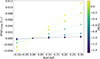 |
Fig. A.1. Variation of the RGBb position in log L as a function of the variation of ΔY/ΔZ for different values of [M/H]. |
Appendix B: Script testing
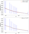 |
Fig. B.1. Variation of the RGBb position in log L (upper panel) and log νmax (lower panel) with the number of stars in the simulation. The red points in the upper panel represent the GCs in our sample. |
To test our analysis method and estimate the systematics due to the number of stars in a sample and the chosen KDE bandwidth, we performed a series of fits on synthetic populations (see Sec. 3.1) generated from the same model (M = 0.8 M⊙, [Fe/H]= − 1.50 dex, [α/Fe]= + 0.4 dex, fov = 0.0), varying each time the number of stars (N⋆) in the simulation and the bandwidth (BW) of the KDE, defined as
 (B.1)
(B.1)
where F is a multiplicative factor which we varied from 0.25 to 1.00. The fit of each F − N⋆ combination was performed 1000 times, to reduce as much as possible numerical effects.
All the results of the fits computed with F = 0.50 (which is the value that we finally adopted for clusters and field stars) were compared with the fit of a reference simulation, generated with a large number of stars (N⋆ = 5000) and a narrow bandwidth (F = 0.25): both for log LRGBb and log νmax, RGBb we obtained that the discrepancy with the reference measurements decays hyperbolically with N⋆, as shown in Fig. B.1. The inferred systematic error for each stellar cluster or bin of field stars was summed quadratically to the random one.
Appendix C: Coefficients of the Mass-Age-Metallicity scaling relation
Coefficients of the Mass-Age-Metallicity scaling relation (eq. 3) for different values of the overshooting efficiency fov.
Coefficients for the scaling relation 3 obtained with different overshooting efficiencies.
All Tables
Properties (age, chemical composition, and reddening) and RGBb luminosities for all the clusters in our sample.
Results of the fits on the fov − [M/H] plane, each one with the corresponding αMLT value and metallicity range.
Coefficients for the scaling relation 3 obtained with different overshooting efficiencies.
All Figures
|
Fig. 1. Left panel: HRD of RGB of NGC 1261, with RGBb stars highlighted in orange and by a blue dashed line referring to the RGBb luminosity obtained from the fit. The errors on log LRGBb already include the systematics due to the number of RGB stars (see Appendix B) and the distance modulus (Baumgardt & Hilker 2018). Right panel: KDE (light blue zone) of luminosity distribution (lower labels) and relative fit (orange line). The blue line represents the histogram of the RGB luminosity with Poissonian errors (upper labels). |
| In the text | |
|
Fig. 2. Comparison between CMDs of NGC 6144 before (left panel) and after (right panel) applying differential reddening correction. |
| In the text | |
|
Fig. 3. Differential reddening map for GC NGC 6144 obtained using HST data sampling radial range up to ∼1.0 half-light radius2. The black cross marks the centre of the cluster (Vasiliev & Baumgardt 2021). |
| In the text | |
|
Fig. 4. Representation in fov − log L plane of interpolation procedure to derive overshooting efficiency for GC NGC 6362. The expectation values of [M/H] and log LRGBb are represented by the solid red line and the dashed black one, respectively, and are plotted on the grid of models computed at the cluster mass (coloured according to metallicity). The light blue shaded zone represents the confidence interval at 68% of the derived overshooting efficiency. |
| In the text | |
|
Fig. 5. RGBb luminosity as function of [M/H] for stellar clusters in our sample (coloured according to MRGBb). The RGBb luminosity decreases with increasing [M/H] and decreasing stellar mass (see e.g. NGC 1261 and NGC 6218). The lines correspond to the RGBb luminosities – at different metallicities – of evolutionary tracks with M = (0.8, 1.17) M⊙ (orange, blue) and fov = 0.000, 0.025 (dotted, dashed). |
| In the text | |
|
Fig. 6. Location of RGBb in log νmax (left) and log L (right) as function of stellar mass, for Kepler stars divided in metallicity bins (orange points). The points coloured from green to blue represent the location of the RGBb in the same metallicity bins for different overshooting efficiencies. The colour-coding for fov is reported in the bottom horizontal bar. |
| In the text | |
|
Fig. 7. Location of RGBb in log νmax (left) and log L (right) as function of metallicity, for Kepler stars divided in mass bins (orange points). The points coloured from green to blue represent the location of the RGBb in the same mass bins for different overshooting efficiencies. The colour-coding for fov is reported in the bottom horizontal bar. Our data are plotted as orange dots, while the results from Khan et al. 2018 are reported as purple stars (left panels). |
| In the text | |
|
Fig. 8. HRD of NGC 6791, with stars observed by Kepler coloured according to νmax. The inset zoomed-in views show the RGBb stars, including the four stars for which we have νmax values from Kepler. The orange and blue lines correspond to the evolutionary tracks with αMLT = 2.090 and αMLT = 2.290, respectively, and no envelope overshooting. |
| In the text | |
|
Fig. 9. Comparison between our RGBb luminosities and those presented in Nataf et al. (2013). |
| In the text | |
|
Fig. 10. Left panel: Teff − log νmax diagram for field stars with M/M⊙ ∈ [0.9, 1.1[ and [M/H]∈[−0.2, 0.0[ dex (grey points) and corresponding evolutionary tracks with αMLT = 2.090 (orange line) and αMLT = 2.290 (blue line). Right panel: Temperature differences between data and evolutionary tracks, with the same colour-coding of the left panel. |
| In the text | |
|
Fig. 11. Overshooting efficiency derived from LRGBb as function of [M/H], both for αMLT = 2.090 (left panel) and αMLT = 2.290 (right panel). Clusters are represented as circles, while field stars are shown as triangles. The blue lines correspond to the linear fits. Points are coloured by stellar mass. |
| In the text | |
|
Fig. 12. Same as Fig. 11, but with the addition of the overshooting efficiencies derived from νmax, RGBb (open symbols) and the relative fits (green lines). |
| In the text | |
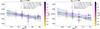 |
Fig. 13. Same as Fig. 12, but only with points for which we computed both fovL and fovνmax. |
| In the text | |
|
Fig. 14. Relative variations of RGBb luminosity and overshooting efficiency for the GC NGC 6362 produced by variations of effective temperature (Teff), metallicity ([M/H]), age (tAge), and distance modulus (dm). |
| In the text | |
|
Fig. 15. Profiles of squared Brunt-Väisälä frequency, N2, for models with M = 1 M⊙ and [M/H]= − 0.5, −0.3, −0.1, +0.1, +0.3 dex. The x-axis is normalised by the position rCE of the convective border, indicated by the vertical dashed black line |
| In the text | |
|
Fig. A.1. Variation of the RGBb position in log L as a function of the variation of ΔY/ΔZ for different values of [M/H]. |
| In the text | |
|
Fig. B.1. Variation of the RGBb position in log L (upper panel) and log νmax (lower panel) with the number of stars in the simulation. The red points in the upper panel represent the GCs in our sample. |
| In the text | |
Current usage metrics show cumulative count of Article Views (full-text article views including HTML views, PDF and ePub downloads, according to the available data) and Abstracts Views on Vision4Press platform.
Data correspond to usage on the plateform after 2015. The current usage metrics is available 48-96 hours after online publication and is updated daily on week days.
Initial download of the metrics may take a while.