| Issue |
A&A
Volume 700, August 2025
|
|
|---|---|---|
| Article Number | A125 | |
| Number of page(s) | 21 | |
| Section | Extragalactic astronomy | |
| DOI | https://doi.org/10.1051/0004-6361/202554144 | |
| Published online | 12 August 2025 | |
The MUSE view of the Sculptor galaxy: Survey overview and the luminosity function of planetary nebulae
1
European Southern Observatory (ESO), Alonso de Córdova 3107, Casilla 19, Santiago 19001, Chile
2
Astronomisches Rechen-Institut, Zentrum für Astronomie der Universität Heidelberg, Mönchhofstraße 12-14, 69120 Heidelberg, Germany
3
Department of Astronomy, The Ohio State University, 140 West 18th Avenue, Columbus, OH 43210, USA
4
Center for Cosmology and Astroparticle Physics, 191 West Woodruff Avenue, Columbus, OH 43210, USA
5
European Southern Observatory, Karl-Schwarzschild Straße 2, D-85748 Garching bei München, Germany
6
Univ Lyon, Univ Lyon1, ENS de Lyon, CNRS, Centre de Recherche Astrophysique de Lyon UMR5574, F-69230 Saint-Genis-Laval, France
7
INAF – Osservatorio Astrofisico di Arcetri, Largo E. Fermi 5, I-50157 Firenze, Italy
8
Finnish Centre for Astronomy with ESO, (FINCA), University of Turku, FI-20014 Turku, Finland
9
Tuorla Observatory, Department of Physics and Astronomy, University of Turku, FI-20014 Turku, Finland
10
Turku Collegium for Science, Medicine and Technology, University of Turku, FI-20014 Turku, Finland
11
Space Telescope Science Institute, 3700 San Martin Drive, Baltimore, MD 21218, USA
12
International Centre for Radio Astronomy Research, University of Western Australia, 7 Fairway, Crawley, 6009 WA, Australia
13
Department of Physics and Astronomy, The Johns Hopkins University, Baltimore, MD 21218, USA
14
Dipartimento di Fisica e Astronomia ‘G. Galilei’, Università di Padova, Vicolo dell’Osservatorio 3, I-35122 Padova, Italy
15
Argelander-Institut für Astronomie, Universität Bonn, Auf dem Hügel 71, 53121 Bonn, Germany
16
Observatories of the Carnegie Institution for Science, 813 Santa Barbara Street, Pasadena, CA 91101, USA
17
Departamento de Astronomía, Universidad de Chile, Camino del Observatorio 1515, Las Condes, Santiago, Chile
18
Department of Astronomy, University of Maryland, College Park, MD 20742, USA
19
Department of Physics and Astronomy, University of Wyoming, Laramie, WY 82071, USA
20
Instituto de Astronomía, Universidad Nacional Autónoma de México, Ap. 70-264, 04510 CDMX, Mexico
21
Department of Physics, University of Connecticut, 196A Auditorium Road, Storrs, CT 06269, USA
22
Universität Heidelberg, Zentrum für Astronomie, Institut für Theoretische Astrophysik, Albert-Ueberle-Str. 2, 69120 Heidelberg, Germany
23
Universität Heidelberg, Interdisziplinäres Zentrum für Wissenschaftliches Rechnen, Im Neuenheimer Feld 225, 69120 Heidelberg, Germany
24
Harvard-Smithsonian Center for Astrophysics, 60 Garden Street, Cambridge, MA 02138, USA
25
Elizabeth S. and Richard M. Cashin Fellow at the Radcliffe Institute for Advanced Studies at Harvard University, 10 Garden Street, Cambridge, MA 02138, USA
26
Max-Planck-Institut für Astronomie, Königstuhl 17, D-69117 Heidelberg, Germany
27
Sub-department of Astrophysics, Department of Physics, University of Oxford, Keble Road, Oxford OX1 3RH, UK
⋆ Corresponding author: This email address is being protected from spambots. You need JavaScript enabled to view it.
Received:
14
February
2025
Accepted:
10
June
2025
Abstract
The Sculptor galaxy, NGC 253, is the southern massive star-forming disk galaxy that is closest to the Milky Way. We present a new 103-pointing MUSE mosaic of this galaxy that covers most of its star-forming disk up to 0.75 × R25. With an area of ∼20 × 5 arcmin2 (∼20 × 5 kpc2, projected) and a physical resolution of ∼15 pc, this mosaic constitutes one of the largest integral field spectroscopy surveys with the highest physical resolution of any star-forming galaxy to date. We exploited the mosaic to identify a sample of ∼500 planetary nebulae (the sample is ∼20 times larger than in previous studies) to build the planetary nebula luminosity function (PNLF) and obtain a new estimate of the distance to NGC 253. The value we obtained is 17% higher than the estimates returned by other reliable measurements, which were mainly obtained via the top of the red giant branch method. The PNLF also varies between the centre (r < 4 kpc) and the disk of the galaxy. The distance derived from the PNLF of the outer disk is comparable to that of the full sample, while the PNLF of the centre returns a distance that is larger by ∼0.9 Mpc. Our analysis suggests that extinction related to the dust-rich interstellar medium and edge-on view of the galaxy (the average E(B−V) across the disk is ∼0.35 mag) plays a major role in explaining both the larger distance recovered from the full PNLF and the difference between the PNLFs in the centre and the disk.
Key words: dust / extinction / planetary nebulae: general / galaxies: distances and redshifts / galaxies: individual: NGC 253
© The Authors 2025
 Open Access article, published by EDP Sciences, under the terms of the Creative Commons Attribution License (https://creativecommons.org/licenses/by/4.0), which permits unrestricted use, distribution, and reproduction in any medium, provided the original work is properly cited.
This article is published in open access under the Subscribe to Open model. This email address is being protected from spambots. You need JavaScript enabled to view it. to support open access publication.
1. Introduction
NGC 253, also known as the Sculptor galaxy, is a massive (Mstar ∼ 4.4 × 10¹⁰ M⊙; Bailin et al. 2011; Leroy et al. 2021) star-forming galaxy located just ∼3.5 Mpc from the Milky Way (Newman et al. 2024; Okamoto et al. 2024). It is also one of the largest galaxies in the sky, with an apparent size of 42 × 12 arcmin2 (Jarrett et al. 2019). With its prominent stellar bar, well-defined spiral arms (Iodice et al. 2014), and its star formation, which is spread throughout the disk, NGC 253 is a nearby archetypal example of a main-sequence spiral galaxy.
Its star formation rate (SFR) has been estimated to be between ∼4.9 (Leroy et al. 2019) and ∼6.5 M⊙.yr−1 (Jarrett et al. 2019). Almost one-third of it (∼2 M⊙.yr−1; Bendo et al. 2015; Leroy et al. 2015) is produced by ten giant molecular clouds that are distributed in a starburst ring (∼500 pc in diameter; Leroy et al. 2015) around its nucleus. This makes this object the closest massive starburst to our Galaxy. In addition, the starburst launches a powerful multi-phase outflow (e.g. Strickland et al. 2000; Bauer et al. 2007; Westmoquette et al. 2011; Bolatto et al. 2013; Walter et al. 2017; Lopez et al. 2023; Cronin et al. 2025) that ejects large amounts of gas (14–39 M⊙.yr−1 for the molecular component only, Krieger et al. 2019) from the centre of the galaxy into its circumgalactic medium. Part of this gas seems to remain in the gravitational well of the galaxy, where it cools down to the neutral phase and moves towards the outskirts of the disk (Lucero et al. 2015), where it might reaccrete and fuel future star formation.
The proximity of the galaxy means that an excellent spatial resolution can be achieved even with ground-based telescopes given the 17 pc.arcsec−1 scale. When it is combined with the large intrinsic size of the galaxy (see Table 1), however, this proximity also results in a large apparent size. Studies in the past decades therefore mostly focused on the smaller central structures, such as the starburst (e.g. Bendo et al. 2015; Leroy et al. 2015) and its related outflow (e.g. Strickland et al. 2000; Bauer et al. 2007; Westmoquette et al. 2011; Bolatto et al. 2013; Walter et al. 2017; Lopez et al. 2023).
Assumed properties for NGC 253.
In this galaxy, individual components of the star formation process (giant molecular clouds, H II regions, their ionising sources) can be resolved. We can observe thousands of sources distributed in a wide variety of environments (in the centre, the bar, the outflow, the spiral arms, and in the inter-arm regions) with a resolution that is better by a factor of 2–5 than for most of the latest integral field unit (IFU) surveys of nearby galaxies (e.g. SIGNALS; Rousseau-Nepton et al. 2018; MAD; Erroz-Ferrer et al. 2019; TYPHOON; Grasha et al. 2022; PHANGS-MUSE; Emsellem et al. 2022), and better by 50–100 times than the previous generation of large IFU surveys (e.g. CALIFA; Sánchez et al. 2012; Husemann et al. 2013; MaNGA; Wake et al. 2017; Bundy et al. 2015; SAMI; Croom et al. 2012).
Large IFU mosaics of extragalactic objects with this high resolution have so far only been obtained for the dwarf galaxies M33 (SIGNALS: Rousseau-Nepton et al. 2019) and for the Magellanic Clouds (Local Volume Mapper: Drory et al. 2024), which sample substantially different properties than those found in a massive system such as NGC 253. The Multi Unit Spectroscopic Explorer (MUSE) additionally observed a few nearby galaxies at high resolution, including NGC 7793 (Della Bruna et al. 2020), M83 (Della Bruna et al. 2022), and NGC 300 (McLeod et al. 2021), but the coverage wassignificantly smaller than our mosaic of NGC 253. While these datasets have comparable if not better spatial resolution, they therefore cannot provide the global view needed to connect small-scale processes with the large-scale properties of galaxies, such as gas flows, diffuse ionised gas (DIG), or interactions with pristine gas.
Several facilities (e.g. ALMA; Leroy et al. 2021, Oakes et al. in prep.; JWST; McClain et al. in prep.; GO2987; PI: Leroy, Congiu, Faesi; HST; Dalcanton et al. 2009, and GO 17809, PI. D. Thilker; MeerKat; Karapati et al. in prep.; MKT-20159, PI: Sardone) have recently invested significant amounts of observing time to map the entire star-forming disk of NGC 253 at the highest possible spatial resolution. Here, we present our new MUSE mosaic of NGC 253. It offers an unprecedented view of its ionised interstellar medium (ISM). This compilation of multi-wavelength data will allow us to explore a wealth of science objectives, starting from the properties, structure, and composition of the multi-phase ISM, to the detailed properties of the stellar populations and the ejection and reaccretion cycle that powers the star formation in the galaxy, to name just a few. The mosaic is composed of 103 unique pointings and is the largest contiguous extragalactic mosaic observed by MUSE so far1. It covers the vast majority of the star-forming disk with an average resolution of 15 pc (∼0.85 arcsec).
In this work, we focused on testing and validating the data by performing an analysis of the planetary nebula luminosity function (PNLF) of the galaxy. Planetary nebulae (PNe) are the final evolutionary stage of intermediate-mass stars (e.g. Kippenhahn et al. 2013). During the post-asymptotic giant branch (AGB) phase, these stars eject their outermost layers, which creates a gaseous nebula and exposes their core (Osterbrock & Ferland 2006). The high temperature of the core (∼100 000 K) results in a hard spectrum that ionises the surrounding gas and creates a PN. For this reason, the (optical) emission spectra of PNe are rich with high-ionisation collisionally excited lines and recombination lines (Osterbrock & Ferland 2006). The strongest of these is the [O III]λ 5007 line, which can account for up to 13% of the total energy emitted by a PN (e.g. Dopita et al. 1992; Ciardullo 2010; Schönberner et al. 2010). Moreover, the ionising source is small, and it produces a limited number of ionising photons. As a consequence, the typical size of a PN is quite small. The largest PNe reach diameters of around ∼1 pc (Acker et al. 1992).
When they are observed at extragalactic distances, PNe appear to be unresolved [O III]λ 5007-bright sources because of these properties. This makes them relatively easy to identify in early-type galaxies, where virtually all [O III]λ 5007 emission is produced by PNe. Moreover, their maximum luminosity has empirically been shown to be constant across galaxies and independent of environment and conditions (e.g. Yao & Quataert 2023) to first approximation. Combined with the easy identification, this property makes PNe ideal candidates for standard candles. Since the late 1980s (Jacoby 1989; Ciardullo et al. 1989), their luminosity function (the PNLF) has been a popular secondary indicator for measuring distances of galaxies within 30 Mpc.
Despite this popularity, the distance of NGC 253 has been estimated by PNLF only twice, by Rekola et al. (2005) and Jacoby et al. (2024). The distances disagree with each other ( Mpc for Rekola et al. 2005 and
  Mpc for Jacoby et al. 2024), but both were based on limited samples. We use our mosaic to identify a new and larger (∼20 times) sample of PNe, build the PNLF for NGC 253, and recover an updated independent estimate of the distance of NGC 253.
In Sect. 2 we describe the observations, the data reduction procedure, and the spectral fitting. Section 3 focuses on the detection, characterisation, and cleaning of the planetary nebulae (PNe) sample, and Sect. 4 describes the fitting of the PNLF and the comparison with the literature findings. Finally, we discuss in Sect. 5 our results, and we summarise them in Sect. 6. Table 1 lists the properties we assumed for this galaxy throughout the paper.
2. Observations and data processing
Most of the data presented in this work were acquired as part of European Southern Observatory (ESO) programme 108.2289 (P.I. Congiu). We used MUSE in its seeing-limited wide-field mode configuration and with the extended wavelength range (WFM-NOAO-E), which covers between 4600 and 9300 Å with a resolution R ∼ 2000 at Hα. The observations were organised in blocks of 2 pointings with three interleaved 120 s sky offset exposures: one at the beginning of each observing block, one between the 2 pointings, and one at the end. We observed four 211 s exposures per pointing (844 s in total), rotating the field by 90 degrees between each exposure to minimise instrumental signatures in the final mosaic. We originally planned for 98 pointings, covering an approximate area of 20 × 5 arcmin2. Three pointings were re-observed because of issues with their positioning, however, which resulted in a final total of 101 pointings and ∼51.5 hours of observing time.
The mosaic also includes two archival pointings that were observed as part of the ESO programme 0102.B-0078 (P.I. Zschaechner). These data were acquired with MUSE in its seeing-enhancing ground-layer adaptive optics wide-field mode configuration and with the extended wavelength range (WFM-AO-E), covering the same wavelength range as our original data. Each pointing has been observed with four 490 s exposures (1960 s in total), with 90-degree field rotations and small offsets between exposures. Two 125 s sky exposures were also acquired using a typical OSOOSO offset pattern. The main differences between these archival data and ours are the longer exposure times and a masked spectral region between 5760 and 6010 Å, introduced to avoid laser contamination. Table B.1 summarises the main properties of the observations, such as the date, the average airmass, the average seeing, and the full width at half maximum (FWHM) of the point spread function (PSF) at 5000 Å, recovered as described in Sect. 3.2.
The final mosaic covers an area of ∼20 × 5 arcmin2 (∼20 × 5 kpc2 at the distance of the galaxy, projected), extending roughly out to 0.75 × R25. This corresponds to around nine million spectra and a final file size of ∼300 GB. Figure 1 shows the reduced mosaic. The top panel shows a colour image produced by combining g-, r-, and i-band images extracted from the datacube. This image highlights the full structure of the galaxy disk, with the prominent bar and complex dust filaments that follow the distribution of the spiral arms of the galaxy. We can also see the change in colour caused by the presence of the central starburst of the galaxy. The bottom panel highlights the gas emission, showing [O III]λ 5007, Hα, and [S II]λλ 6717,6731, showing off the multitude of ionised gas structures we observe in the galaxy. The H II regions distribution highlights the structure of the spiral arms, while the [O III]λ 5007 and [S II]λλ 6717,6731 emission clearly show the outline of the outflow. Nebulae withdifferent properties can be identified across the field, like the blue, [O III]λ 5007 emitting PNe, the green Hα bright H II regions, and the pink, [S II]λλ 6717,6731 emitting supernova remnants(SNRs).
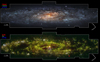 |
Fig. 1. Colour images of NGC 253 produced by combining broad-band images and emission-line maps extracted from the MUSE data cube. The mosaic covers an area of 20 × 5 arcmin2, and it includes roughly nine million independent spectra. The top panel shows a composition of three broad-band filters. The g band is plotted in blue, the r band in green, and the i band in red (Acknowledgement: ESO/M. Kornmesser). The bottom panel is a composition of emission line maps with [O III]λ 5007 in blue, Hα in green and [S II]λλ 6717,6731 in red. |
2.1. Data reduction
All data were reduced using pymusepipe, which is a Python wrapper of the ESO MUSE pipeline (Weilbacher et al. 2020) presented by Emsellem et al. (2022). The reduction procedure followed the one described for the MUSE data of the Physics at High Angular Resolution in Nearby GalaxieS (PHANGS) collaboration in the latter work. We highlight some significant differences in the following paragraphs.
2.1.1. Alignment
The astrometry provided by the MUSE pipeline is not accurate enough to combine multiple exposures into a large mosaic. Emsellem et al. (2022) addressed this by manually aligning each exposure to a reference R-band image from the PHANGS-Hα survey (Razza et al. in prep.). They extracted broad-band images from the MUSE cubes using the PHANGS-Hα filter transmission curve, and aligned them by applying sub-pixel shifts and rotations to match the reference image.
While effective, this method is time consuming and somewhat subjective. We instead used a semi-automatic routine based on the spacepylot package2, which employs optical flow to determine alignment corrections. This technique compares two images of the same object and computes the vector field required to transform one into the other. spacepylot then averages these vectors to derive global shifts and rotations, which we applied to individual exposures followingEmsellem et al. (2022).
NGC 253 was not part of the PHANGS-Hα survey, but several Wide Field Imager (WFI) R-band images are publicly available in the ESO archive. We reduced them using the pipeline of Razza et al. (in prep.) and Emsellem et al. (2022), and used the resulting R-band mosaic as our astrometric reference. This image was aligned to the Gaia Data Release 2 (Gaia Collaboration 2018; Lindegren et al. 2018). Comparing stellar positions in the WFI image with Gaia, we found astrometric offsets of 0.02 ± 0.60 arcsec in right ascension and 0.03 ± 0.46 arcsec indeclination.
2.1.2. Sky subtraction
The sky subtraction is the most critical step in this data reduction. When observing extended targets with MUSE, the typical strategy is to regularly observe an empty sky field close to the target. The MUSE pipeline’s standard sky subtraction routine3 (Weilbacher et al. 2020) uses these sky exposures to build a model of the sky emission, separating it into continuum and emission-line components. The continuum component is directly subtracted from the science exposures. Emission lines, instead, are grouped by physical origin, compared to the faintest spaxels in the science frames, re-scaled, and then subtracted. This allows for improved sky subtraction, especially considering that some of these line groups (e.g. [O I], OH) vary significantly on short timescales and can result in significant artefacts if not treated carefully.
This strategy works well for most extragalactic targets, which typically have a significant redshift. NGC 253, however, is a very local source, with a systemic line-of-sight velocity of vsys ∼ 242 km.s−1 and a rotation curve of ±200 km s−1 (Hlavacek-Larrondo et al. 2011). This means that the approaching side of the galaxy has a relative velocity of only ∼40 km s−1, and that some of the target’s lines fall very close to their atmospheric counterparts (Fig. 2). Since this velocity difference is just below the instrument resolution of ∼50 km s−1 at Hα, the pipeline cannot reliably separate sky and target emission, resulting in the over-subtraction of such lines unless they are are not tied to a larger group. This issue affects mostly the [O I] lines (especially [O I]λ 6300, [O I]λ6363, and [O I]5577) and the hydrogen Balmer lines (Hα and Hβ). While the [O I] lines are among the most variable in the night sky (produced by atmospheric atoms excited through collisions with charged particles; Bates 1946; Solomon et al. 1988), the Balmer lines are more stable (caused by high-atmosphere hydrogen excited by solar Lyα; Nossal et al. 2019). Because their intensity varies slowly on the 5–10 minute scale between sky and object exposures, the Balmer lines can be treated as constant during this interval. This is especially important because they are two of the most important lines in the ionised gas spectrum. We were able to recover their flux from the dedicated sky exposures and subtract it directly from the science frames. To enable this, we excluded Hα and Hβ from the pipeline’s list of fitted sky emission lines, forcing them to be treated as part of thecontinuum.
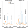 |
Fig. 2. Hα region of the spectra in two different regions of the galaxy. The left panel represent the approaching side of the galaxy, and the right panel shows the receding side. In both panels we show in blue the spectrum extracted from the science exposure after our updated sky subtraction procedure, in orange the sky spectrum associated with the exposure, while the grey dashed lines represent the expected position of Hα at v = 0 km/s. |
In addition, we identified several pointings with an asymmetric and unphysical Hβ absorption profile (Fig. 3). This was an artefact caused by the overfitting of sky lines near the Hβ region. Since the Paranal sky spectrum does not contain bright lines at λ < 5000 Å (Hanuschik 2003), we solved the issue by excluding all sky lines bluer than 5000 Å from the pipeline’s list. This removed ∼9000 lines, almost 40% of the full list. Figure 3 shows a comparison between the original spectrum (blue) and the corrected one (orange). Although not all exposures are affected by these issues, we applied the improved sky subtraction procedure to the entire dataset for consistency. We then combined all reduced exposures into the final mosaic following the method of Emsellem et al. (2022).
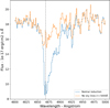 |
Fig. 3. Hβ region of the spectra in a circular aperture of 4 arcsec extracted from one of the pointings with an asymmetric Hβ profile. The blue line represents the spectrum obtained from the normal sky subtraction, while the orange line shows the spectrum obtained after removing the sky lines with wavelengths shorter than 5000 Å from the line list used to build the sky model from the dedicated sky offset. The vertical, dashed, grey line, represents the expected position of the Hβ emission line, considering the rotation curve of the galaxy. |
2.2. Spectral fitting
We processed the data with the PHANGS data analysis pipeline4 (DAP) to compute the properties and kinematics of the underlying stellar population, subtract their continuum from the spectra, and extract the flux of the main emission lines. The DAP is described in detail in Emsellem et al. (2022), but here we summarise the main features relevant to this work. The DAP runs the spectral fitting routine, based on the ppxf package (Cappellari 2017), three times. The first run is performed on Voronoi-binned data using a reduced set of simple stellar population models from the Extended Medium resolution INT Library of Empirical Spectra (E-MILES) library (Vazdekis et al. 2016) to characterise the stellar kinematics across the galaxy. The second run uses the same Voronoi-binned spectra, keeps the kinematics fixed from the first step, and employs a more extensive library of simple stellar population models (also from the E-MILES library Vazdekis et al. 2016) to extract additional stellar population parameters (e.g. age, metallicity). Finally, a third run is performed on each individual spaxel to remove the stellar continuum and simultaneously fit the emission lines with Gaussian profiles. The kinematics of the stellar templates is fixed from the first step, and the reduced template sample is used for the fit. Emission lines are grouped into three sets with fixed kinematics (see Sect. 5.2.5 of Emsellem et al. 2022). At the end of the process, the final results are compiled in a multi-extension FITS file, the MAPS file, which contains two-dimensional maps of all fitted parameters. The physical quantities in the output files are summarised in Table B.4, while Table B.3 lists the emission lines included in the fit.
We also extracted moment-zero, -one, and -two maps of the main emission lines to recover more complete flux and kinematics information in regions where the DAP’s single-Gaussian fit is insufficient to represent the real line profile (e.g. the galaxy centre). All maps were extracted from continuum-subtracted cubes produced by the DAP using an extraction window of ± 500 km s−1 around the recession velocity of the galaxy. The only exception is the [S II]λλ 6717,6731 doublet, for which we used a larger extraction window (±750 km s−1) centred on the average wavelength of the two lines, to avoid cross-contamination. In this case, we recovered only the moment-zero map and its associated error map.
3. Analysis
3.1. Detection of the planetary nebula candidates
Planetary nebulae in galaxies outside the local group appear as [O III]λ 5007-bright point sources due to their small physical size (< 1 pc, e.g. Acker et al. 1992) and the high degree of ionisation of their gas. As a result, all common PNe identification techniques, such as image “blinking” (e.g. Jacoby 1989), automatic point source detection (e.g. Scheuermann et al. 2022), colour-magnitude diagram analysis (Arnaboldi et al. 2002), or differential emission-line filtering (Roth et al. 2021), focus on analysing [O III]λ 5007 emission line maps in various forms.
We detect our PN candidates using a visual approach based on the [O III]λ 5007, Hα, and [S II]λλ 6717,6731 moment maps (Fig. 4). We used both an RGB image combining the three maps (blue for [O III]λ 5007, green for Hα, and red for [S II]λλ 6717,6731) and the individual Hα and [O III]λ 5007 maps. We first selected as PN candidates all sources in the [O III]λ 5007 map that appeared point-like and lacked a bright counterpart in the Hα map. The RGB map was then used to clarify borderline cases, such as PNe near bright H II regions or objects with detectable Hα emission but still appearing bluer than typical H II regions. The colour map clearly highlights PNe as blue dots even in crowded areas or when their emission is faint and hard to identify in the [O III]λ 5007 map. Ambiguous sources were included in the catalogue, relying on the methods in Sect. 3.4 for potential rejection via a quantitative approach. We removed from the catalogue all sources for which reliable [O III]λ 5007 photometry was not possible, either due to proximity to other [O III]λ 5007-emitting sources (mainly other PN candidates) or location at the edge of themosaic.
 |
Fig. 4. Example of the different images we used to visually detect nebulae. We show zoom-ins of four different areas of the galaxy. For each region, we show on the top the three colour map (same colours as in Fig. 1, bottom panel), in the middle the [O III]λ 5007 and in the bottom the Hα map. The circles highlight the position of nebulae in the final catalogue, with the solid circles showing the position of confirmed PNe and dotted ones showing nebulae classified either as supernova remnants or as compact H II regions. White triangles show the position of the objects identified by DAOFIND, which are, for the most part, spurious detections. |
We also tested an alternative detection method based on DAOFIND (Stetson 1987), successfully used by other authors under similar conditions (e.g. Scheuermann et al. 2022). This algorithm is quick and semi-automatic but assumes a uniform PSF across the field of view (FOV), which is not the case here (see Sect. 3.2), and cannot exploit colour information as effectively as visual inspection. We applied the photutils (Bradley et al. 2024) implementation of DAOFIND to the [O III]λ 5007 moment-zero map to generate an alternative PN candidates list. We tried several combinations of the main parameters (thresholds, FWHM, sharpness, and roundness), but none yielded satisfactory results. The software was detecting ∼10 000 objects, which visual inspection showed to be spurious detections or bright spots clearly associated with H II regions. Even after removing contaminants (as described in Sect. 3.4), more than half of these sources were still identified as PNe. We therefore opted to continue the analysis using the visually compiled catalogue. Appendix A discusses the results of the PNLF using the DAOFIND-based catalogue.
Visual detection can be subjective, however, and the final candidate list may vary depending on who performed the selection. To reduce this bias, three co-authors (E.C., C.T., and T.K.) independently carried out the detection procedure. Their catalogues were merged into a single compilation. Duplicates were removed by comparing coordinates, merging sources close enough to likely be the same object. We then conducted a second check for sources near each other that might cross-contaminate their photometry. The final catalogue includes 832 PN candidates. Table 2 summarises its composition and that of each person’s original sample.
Summary of the PN candidates identified in the paper.
3.2. Point spread function
To obtain reliable photometry of our sources, we need a good characterisation of the PSF of the data. It is essential to both select an adequate aperture for the photometry and apply a precise aperture correction. The observations of NGC 253 were performed using ∼53 OBs (including archival ones) that were acquired between 2018 and 2022 under a wide variety of sky conditions, however (Table B.1). As a result, the PSF can change significantly across the mosaic.
A common way to characterise the PSF of astronomical data is to fit bright sources across the FOV of the instrument with a model of the PSF. Unfortunately, only a handful of OBs included bright foreground stars that could be used to reliably characterise it, so we devised an alternative method. Given their properties, PNe are ideal for characterising the local PSF. They are faint, but the shape of the MUSE-WFM PSF is relatively well studied, and this “a priori” knowledge can be used to decrease the number of free parameters and improve fit reliability. In particular, the PSF can be modelled quite well by a circular Moffat profile (Moffat 1969), characterised, to the first approximation, by a constant power index (2.8 for the NOAO mode and 2.3 for the AO mode Hartke et al. 2020; Emsellem et al. 2022) and variable full width at half maximum (FWHM).
We fitted each PN candidate identified in Sect. 3 with a circular Moffat profile with fixed power index and recovered their FWHM, which we include in the catalogue of PN candidates available through Vizier. The fit was performed using the [O III]λ 5007 moment zero map. In the following analysis, we consider their FWHM as the FWHM of the local PSF at ∼5007 Å, the wavelength of the [O III]λ 5007 emissionline.
Finally, we take the clean sample of PNe described in Sect. 3.4 to estimate the average FWHM of each pointing in which at least one confirmed PNe is present. We used the clean sample to ensure only confirmed point sources are considered. We report the estimates in Table B.1. The average PSF FWHM of our observations is therefore 0.8 arcsec (measured from 100 individual pointings), which corresponds to 13.5 pc, with a standard deviation of 0.2 arcsec. The maximum FWHM is 1.6 arcsec (27 pc) and the minimum is 0.49 arcsec (8.5 pc).
3.3. Aperture photometry
We used photutils to perform aperture photometry of our candidates using moment-zero maps of several emission lines: [O III]λ 5007 to build the PNLF, and Hα, [N II]λ 6584, and [S II]λλ 6717,6731 to reject contaminants (H II regions, SNRs) in the sample. We adopted apertures with diameters equal to the FWHM of the local PSF (see Sect. 3.2). Then, we estimate the local background emission in an annulus with an inner diameter of 4×FWHM and an area of five times that of the central aperture. To remove the flux component caused by the diffuse emission of the galaxy, we rescaled this background for the difference in size between apertures and subtracted it from the integrated fluxes of the objects. Since the apertures we adopted are small, we leveraged the FWHM of the local PSF to calculate the appropriate aperture correction for each PN5. The PSF fit was performed on the [O III]λ 5007 moment-zero map, so we adjust the correction according to the wavelength of the considered line to account for the PSF size’s wavelength dependence (as described in Emsellem et al. 2022).
We then corrected for Galactic extinction, using a Cardelli et al. (1989) extinction law with R(V) = 3.1 and an E(B−V) of 0.0165 (Schlafly & Finkbeiner 2011). We did not correct for internal extinction, for the reasons we discuss in Sect. 5.4. Finally, we converted the [O III]λ 5007 fluxes (in erg.cm−2.s−1) to apparent magnitudes using the following equation from Jacoby (1989):
 (1)
(1)
We estimated errors on the integrated fluxes using the moment-zero error maps and standard error propagation. We also add in quadrature a 0.11 mag error on the [O III]λ 5007 magnitudes, which we estimate as the typical uncertainty on the aperture correction from our analysis in Sect. 5.1.
3.4. Contaminants
The next step was to clean our sample of PN candidates from contaminants. This is particularly important in a star-forming galaxy like NGC 253 where PNe are a minority of the [O III]λ 5007-emitting sources. The two most common contaminants are SNRs and compact H II regions. To remove them from our catalogue, we leverage the different spectral properties of the three classes of sources. H II regions and PNe are both powered by photoionisation, but the former are ionised by O or B stars that produce a soft ionising spectrum with respect to the white dwarfs typically powering PNe. For H II regions, this results in a spectrum dominated by hydrogen recombination lines (Hα in particular) and other lines from moderately low ionisation ions (e.g. [N II]). Planetary nebulae spectra, on the other hand, are dominated by highly ionised forbidden lines, like [O III]λ 5007, and recombination lines, such as He IIλ 4685. Finally, supernova remnants are mostly powered by shocks, which enhance low-ionisation lines like the [O I]λ 6300 and [S II]λλ 6717,6731 doublets.
Several methods have been developed in the literature to take advantage of these properties to classify these nebulae. We exploited the two most common methods. To reject H II regions, we leveraged the criterion developed by Ciardullo et al. (2002) and Herrmann et al. (2008),
![Mathematical equation: $$ \begin{aligned} \log _{10} \frac{I_{5007}}{I_{\mathrm{H} \alpha +[\mathrm{N} \,ii ]\,\lambda 6583}} > -0.37 M_{5007} - 1.16 , \end{aligned} $$](/articles/aa/full_html/2025/08/aa54144-25/aa54144-25-eq4.gif) (2)
(2)
while for SNRs, we applied the traditional D’Odorico et al. (1980) criterion,
![Mathematical equation: $$ \begin{aligned} \log _{10} \frac{I_{[\mathrm{S} \,ii ]\,\lambda 6717 + [\mathrm{S} \,ii ]\,\lambda 6731}}{I_{\mathrm{H} \alpha }} > -0.4. \end{aligned} $$](/articles/aa/full_html/2025/08/aa54144-25/aa54144-25-eq5.gif) (3)
(3)
Kopsacheili et al. (2020) and Li et al. (2024) showed how an [O I]λ 6300 based criterion is more effective at identifying SNRs from H II regions. The [O I]λ 6300 line in our data is heavily compromised by sky emission, however, and we are not interested in a clean sample of SNRs, so we stuck with the criterion in Eq. (2). During the classification, we consider the flux of non-detected lines equal to its uncertainty. We also checked for overluminous sources, that is, sources that look like PNe but that are significantly brighter than the bright cutoff of the PNLF (Longobardi et al. 2013; Hartke et al. 2017; Roth et al. 2021; Scheuermann et al. 2022), without finding any of them in our sample. Finally, we exploited the size recovered in the previous section, to reject five objects that are either too large (FWHM > 2 arcsec) or too small (FWHM < 0.2 arcsec). The first criterion rejects extended sources, since all our data were acquired with seeing ∼1.2 arcsec or better. The second one rejects bad pixels and similar artefacts that can be confused with real sources at first glance.
After all these checks, our clean sample of PNe includes 571 objects. Figure 5 shows the position of the confirmed PNe in the [O III]λ 5007 emission line map. Of the remaining 253 regions (without counting the 5 regions rejected for their size), 200 are classified as H II regions, while 53 as SNRs. The catalogue of sources, which contains all the information reported in Table B.2, is available through CADC and Vizier.
 |
Fig. 5. [O III]λ 5007 line map of NGC 253. The empty circles mark the location of confirmed PNe. The dashed grey ellipses represent the boundary we used to define the radial bins presented in Sect. 5.2. |
4. The planetary nebula luminosity function in NGC 253
The PNLF, that is, the number of PNe observed as a function of their [O III]λ 5007 luminosity, is commonly described by an empirical relation, an exponential distribution truncated at the bright end (Ciardullo et al. 1989)
 (4)
(4)
where M5007* denotes the absolute [O III]λ 5007 magnitude of the brightest possible PN, that is, the zero-point of the luminosity function. Its value is calibrated using galaxies with distances known from primary indicators such as Cepheids or the tip of the red giant branch (TRGB).
Typical estimates place M5007* around −4.5 mag, with −4.54 mag from Ciardullo et al. (2013) being the most widely adopted. While a mild metallicity dependence has been reported (e.g. Ciardullo et al. 2002; Bhattacharya et al. 2021; Scheuermann et al. 2022), its significance remains uncertain. Given that NGC 253 has near-solar metallicity (12 + log(O/H) = 8.69; Beck et al. 2022), where the empirical metallicity dependence is nearly flat, we ignore this dependence and consider M5007* = −4.54 mag throughout our analysis.
We fit Eq. (4) to our data using the maximum likelihood approach of Scheuermann et al. (2022). Figure 6 shows the resulting PNLF (left) and its cumulative form (right). To avoid incompleteness effects at the faint end, we impose a magnitude cutoff based on visual comparison of three independently compiled PN samples (E.C., T.K., C.T.). Figure 7 shows that all three samples begin to drop at ∼25.5 mag. While a real decline in PN counts is expected ∼2 mag below the bright end (e.g. Jacoby & De Marco 2002; Reid & Parker 2010; Ciardullo 2010; Rodríguez-González et al. 2015; Bhattacharya et al. 2021), our model does not account for this feature. We therefore restrict the fit to the 320 PNe brighter than 25.5 mag. The fit returns a distance modulus of  mag (
mag ( Mpc).
Mpc).
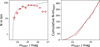 |
Fig. 6. PNLF and cumulative PNe [O III]λ 5007 luminosity function for NGC 253. The red points show the measured PNLF and cumulative function, and the dashed black line represents the best-fit model. The empty points mark the bins of the PNLF that were not considered in the fit. |
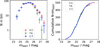 |
Fig. 7. Comparison between the luminosity functions obtained from the three individual samples described in Sect. 3.1. The left panel shows the PNLFs, while the right panel shows the cumulative luminosity function. The figure shows how the three samples significantly overlap at the bright end, while the number of PNe drops in all cases around 25.5 mag. |
Figure 8 compares the distance from our analysis to previous results from the literature6. Our measurement, shown as a solid black vertical line, is accompanied by shaded regions indicating the 1σ (dark grey) and 3σ (light grey) uncertainties. It stands out as significantly larger than most previously reported values. The commonly accepted distance to NGC 253 is ∼3.5 Mpc, with the most recent estimates reported by Newman et al. (2024) and Okamoto et al. (2024) via TRGB analysis. Our measurement exceeds this value by ∼0.35 mag (0.6 Mpc), with only two similar distances found in Willick et al. (1997), based on InfraRed Astronomical Satellite (IRAS) satellite data and the Tully-Fisher (TF) relation (Tully & Fisher 1977). Among the compiled distances, we have two other measurements via the PNLF: Rekola et al. (2005) and Jacoby et al. (2024). In the following, we compare our result directly with these two studies.
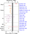 |
Fig. 8. Comparison between our measurement (solid vertical black line) with errors (1σ, dark colour, and 3σ, lighter colour) with distances from the literature. All measurements are divided depending on the method used. Distances from: Bottinelli et al. (1986), Tully & Fisher (1988), Davidge & Pritchet (1990), Davidge et al. (1991), Tully et al. (1992), Willick et al. (1997), Rekola et al. (2005), Dalcanton et al. (2009), Jacobs et al. (2009), Tully et al. (2009), Radburn-Smith et al. (2011), Tully et al. (2013), Jacoby et al. (2024), Newman et al. (2024), Okamoto et al. (2024). |
4.1. Comparison with Rekola et al. (2005)
Rekola et al. (2005) were the first to measure the distance of NGC 253 using the PNLF method through ground-based [O III]λ 5007 and Hα narrow-band images acquired with FORS. Of the 24 PNe they detected, they selected the 14 brightest ones for the PNLF fit and obtained a distance of  mag (
mag ( Mpc). Of these 14 PNe, 12 have counterparts in our sample7. We classify all of them as PNe, except one, the brightest in the Rekola et al. (2005) sample, that we classify as an H II region.
The blue circles in Fig. 9 show the difference between our photometry and Rekola et al. (2005), with solid markers denoting the sources used in their PNLF fit and open circles indicating the ones they excluded but that are within our mosaic. Their Milky Way extinction correction slightly differs from ours. To ensure consistency in the comparison, we recalculated our extinction correction using E(B − V) = 0.019, RV = 3.07, and a Fitzpatrick (1999) extinction law. There is a scatter of 0.4 mag between the two works, but without a significant offset (0.06 mag). This implies that there is no systematic difference between the two sets of measurements. The observed scatter may be related to the different observing techniques and the inherent challenge of obtaining precise photometry for dim objects against a complex background emission, such as that present in NGC 253.
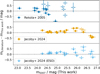 |
Fig. 9. Comparison between our PNe photometry and that of Rekola et al. (2005) and Jacoby et al. (2024). For Jacoby et al. (2024), we performed the comparison using both the data reduced by us, and the cubes directly recovered from the ESO archive. Solid symbols represent PNe that were used by the original authors in their PNLF computation. Open symbols represent objects that were not included in the final fit. |
To confirm that the difference in photometry does not influence the distance of the galaxy, we perform the fit of the PNLF using only the 12 sources in common between the two samples. We measure a distance modulus of  mag (
mag ( Mpc). This value is slightly smaller, but still within the error bars of Rekola et al. (2005) original measurement, confirming that the difference in photometry is not the cause of the discrepancy. We highlight, however, that we include in this fit the object we classify as an H II region. Given the small number of PNe, the PNLF distance is particularly sensitive to the magnitude of the brightest objects, and this nebula is significantly brighter than the second brightest one in both samples (0.34 mag according to Rekola et al. 2005 photometry and 0.77 mag according to our photometry). Therefore, we repeated the analysis removing this object from the sample, obtaining a distance modulus of
  mag (
mag ( Mpc). Although the errors are large, the value is consistent with what we recover from the full sample, confirming that the discrepancy between our results and those reported in Rekola et al. (2005) is mainly driven by the misclassification of this single object.
4.2. Comparison with Jacoby et al. (2024)
Jacoby et al. (2024) recently estimated the distance of NGC 253 via the PNLF using the two archival MUSE pointings from programme 0102.B-0078 (P.I. Zschaechner). Their analysis employs the differential emission line filter method introduced by Roth et al. (2021) to identify PN candidates. This method comprises two steps: first, generating continuum-subtracted maps for each spectral channel within a specific wavelength range centred on the [O III]λ 5007 line; second, detecting PN candidates by combining three wavelength-adjacent maps and selecting point sources that appear consistently across at least three of them. Despite the small area covered by the data, they were able to identify 34 PNe and estimate a distance modulus of  mag (
mag ( Mpc). This is one magnitude (∼2 Mpc) larger than the typically accepted value. They note that the archival MUSE pointings cover a suboptimal region for PNLF studies, the galaxy’s centre, where gas and dust structures complicate PNe identification and hinder precise photometry, likely leading to an overestimated distance. Nevertheless, we proceed with the comparison since it could still provide an important validation of our results.
We have included the same MUSE archival data in our mosaic, so all PNe identified by Jacoby et al. (2024) are included in our footprint. We identify in our catalogue only 21 of their 34 objects, and all of them are classified as PNe, except one (which we consider a SNR). Visual inspection suggests that most of the remaining 13 sources are either extremely faint in our [O III]λ 5007 map or appear as knots within the outflow-related [O III]λ 5007 emission. One exception is a source at the edge of the southern pointing, excluded from our catalogue because it appears as a pair of close candidates, making reliable photometry unfeasible. The orange points in Fig. 9 illustrate the photometric comparison between the two works. The scatter (0.17 mag) and offset (0.07 mag) are similar to those found in the comparison with Rekola et al. (2005), though the residuals reveal some structured trend, hinting at possible systematic differences.
Jacoby et al. (2024) used for their analysis the reduced version of the data publicly available through the ESO archive, which uses a different approach to the sky subtraction and exposure alignment. To assess whether this affects the measurements, we repeated our analysis using these publicly available cubes and found no significant difference for the brightest sources (Fig. 9, light blue triangles).
Following the same approach used for Rekola et al. (2005), we attempted to reproduce the Jacoby et al. (2024) PNLF using only the sources common to both catalogues8. Using all the sources we have in common, we obtain a distance of  mag (
mag ( Mpc). If we remove the two sources that were not used by Jacoby et al. (2024) in their fit, the result changes to
  mag (
mag ( Mpc).
Mpc).
Our photometry yields generally fainter magnitudes than those in Jacoby et al. (2024), leading to a slightly smaller distance estimate. The errors are quite large, however, so that the result is still within 1σ of their measurement. Moreover, this distance is significantly larger than what we obtain using our full PNe sample, supporting the interpretation by Jacoby et al. (2024) that the brightest PNe in the galaxy centre are likelymissing.
This exercise demonstrates two things. First, it shows that, even though our photometry shows some difference with respect to other measurements available in the literature, this does not significantly influence the distances recovered by the PNLF when limiting our analysis to the sample in common with previous works, and that therefore our result is reliable. Secondly, it shows that the Rekola et al. (2005) estimate of the distance of the galaxy, the only one in agreement with the commonly accepted TRGB-based value, is driven by the misclassification of one object. Therefore, all PNLF-based measurements of the distance to this galaxy are significantly overestimated compared to the TRGB-based distances. In the next section, we will investigate the possible origin of this tension.
5. Discussion
As we introduced in Sect. 4, the distance modulus we obtain from our analysis is 0.35 mag (0.6 Mpc) larger than what is recovered by other methods (mostly TRGB, ∼27.72 mag, ∼3.5 Mpc, Jacobs et al. 2009; Dalcanton et al. 2009; Radburn-Smith et al. 2011; Okamoto et al. 2024; Newman et al. 2024). Given the good reported agreement between these two methods in past work (e.g. Roth et al. 2021; Scheuermann et al. 2022; Jacoby et al. 2024), this discrepancy was unexpected. Figure 10 shows a direct comparison between TRGB and PNLF distances recovered from the NASA Extragalactic Database (NED) Redshift-Independent Distances database9. Since the database was last updated in 2020, it does not include more recent MUSE-based PNLF measurements. We therefore supplement the plot with additional distances published in Anand et al. (2021), Roth et al. (2021), Scheuermann et al. (2022), Jacoby et al. (2024), and Anand et al. (2024). The figure illustrates that TRGB- and PNLF-based distances follow a tight relation out to ∼15 Mpc10. Beyond 15 Mpc, only a handful of MUSE-based PNLF measurements are available, with increased scatter driven primarily by NGC 1433 and NGC 1512. As discussed by Scheuermann et al. (2022) and Jacoby et al. (2024), these deviations are linked to the misidentification of the TRGB in their colour-magnitude diagrams (CMD).
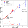 |
Fig. 10. Distance comparison for galaxies with PNLF and TRGB measurements from NED. The red points indicate galaxies where the PNLF was measured using imaging techniques, while blue points indicate PNLF measurements obtained with MUSE data. The grey line shows the one-to-one relation. The orange and light blue triangles identify the position of NGC 253 in the diagram when considering only imaging PNLF or MUSE-based PNLF, respectively. Error bars represent the range between the minimum and maximum values obtained via a specific method. We also annotated in the main panel the position of a few notable sources, and we plot Pegasus, Leo A, and WLM with open red circles. |
In contrast, this explanation does not hold for NGC 253. Its distance is significantly lower, making it easier to identify the position of the TRGB in the CMD. In fact, its TRGB-based distance has been independently measured multiple times in the literature (Jacobs et al. 2009; Dalcanton et al. 2009; Radburn-Smith et al. 2011; Okamoto et al. 2024; Newman et al. 2024), and all estimates are in mutual agreement. On the other hand, the PNLF is not an easy method to apply to star-forming galaxies, where most of the [O III]λ 5007 emission is produced by other types of nebulae. Additionally, there are known cases where the PNLF yields inconsistent distances depending on the region of the galaxy sampled (Herrmann et al. 2008; Bhattacharya et al. 2021). Several observational effects, such as extinction, background subtraction, and aperture correction, can impact the photometry of PNe and hence the distance derived from the PNLF. In the following section, we examine these factors in more detail to investigate the origin of the discrepancy.
5.1. Aperture correction
The aperture correction is one of the most critical aspects of our analysis. It is essential to recover the full flux of a point-like source when a small aperture, which does not encompass the entirety of the PSF, is used to perform photometry. Good aperture corrections should provide the same total flux for the same object regardless of the aperture size.
To assess whether the aperture correction could account for the discrepancy in our distance estimate, we conducted a series of validation tests. First, we repeated the photometry using apertures with diameters 2 and 3 times larger than the originals, and applying the corresponding aperture corrections. We then compared the resulting fluxes to our original measurements. We evaluated that doubling the diameter results in fluxes that are, on average, only 2% higher, with a standard deviation of 6%. Instead, tripling the diameter produces fluxes that are 3% higher on average, but with a slightly larger standard deviation (12%). The small average differences indicate that the aperture correction performs well overall, although the increased scatter suggests some object-to-object variability. Fig. 11 shows, however, that the scatter is negligible for the brightest objects, which means that the effect of the aperture correction on the distance estimate is negligible as well.
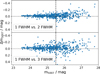 |
Fig. 11. Effect of the aperture correction on the measured magnitude of the PNe in our sample. Only the objects brighter than 25.5 mag (vertical dashed line) have been used for the PNLF fit. We define Δ[OIII] as m(X × FWHM)−m(FWHM) with X being either 2 or 3. |
To confirm this, we used the new photometry to recompute the galaxy’s distance. We obtain a distance modulus of  mag (
mag ( Mpc) when using the 2×FWHM apertures and
  mag (
mag ( Mpc) when using the 3×FWHM apertures. The final result is, in both cases, within 1σ of our original measurement (
 mag or
  Mpc). We therefore conclude that, although our aperture correction method introduces some scatter, its effect on the final distance modulus is minimal and limited to at most 0.05 mag.
5.2. Radial variation in the PNLF
The PNLF has generally been found to be stable when selecting subsamples of PNe located in different regions of a galaxy (e.g. Hui et al. 1993; Ciardullo et al. 2004, 2013). Some exceptions were observed in the halo (e.g. M31; Bhattacharya et al. 2021) and within galaxy disks (e.g. Herrmann et al. 2008), however. The comparison we performed in Sect. 4.2 suggests that a radial dependence of the PNLF may also be present in NGC 253, as the distance recovered from PNe located in the central regions is significantly larger than that obtained using the full population.
To further explore a potential environmental dependence, we divided our PNe into subsamples based on their deprojected distance from the galaxy centre. We deproject the position of each object using the parameters listed in Table 1, which are adopted from the HyperLEDA catalogue (Makarov et al. 2014) and McCormick et al. (2013), and a standard distance of 3.5 Mpc (e.g. Okamoto et al. 2024). We then defined three subsamples: the first includes PNe located within the central 4 kpc of the galaxy; the second contains those between 4 kpc and 8 kpc; and the third includes all objects beyond 8 kpc. These boundaries were chosen to divide the galaxy’s semi-major axis into roughly equal parts while ensuring that each bin contains a sufficient number of PNe brighter than 25.5 mag (∼100) to allow a reliable fit of the PNLF (see Table 3).
Summary of the three distance-based samples and results of the fit.
The result of the analysis is reported in Fig. 12. The plot shows that the central PNLF is almost 0.75 mag fainter than that obtained from the other two samples. As a consequence, the distance is significantly larger ( mag, or
  Mpc), and it agrees with the value we derived in Sect. 4.2. The other two PNLFs appear mutually consistent, although the 4–8 kpc sample contains a larger number of sources. Indeed, the distance moduli we recover are
  mag (
mag ( Mpc) and
  mag (
mag ( Mpc) for the 4–8 kpc and > 8 kpc samples, respectively.
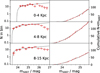 |
Fig. 12. PNLF for the three PN subsamples at different galactocentric distances. The left column shows the PNLF and their fit, and the right column shows the cumulative luminosity function. The colours and symbols are the same as in Fig. 6. |
We performed a k-sample Anderson-Darling test for each pair of sub-samples. The results are reported in Table 4, and they confirm that the central sub-sample is statistically inconsistent with being drawn from the same parent distribution as the other two sub-samples at high significance levels (1% and 3%, respectively), while the two outer sub-samples are fully consistent with being drawn from the samedistribution.
Results of the K-sample Anderson-Darling test applied to each pair of sub-samples.
Comparing the distances obtained from these sub-samples with the measurement we performed using the full sample shows that excluding the central PNe changes the final measurement only marginally. This is somewhat expected, since the distance measurement is mostly driven by the brightest nebulae and, as is clear from Fig. 12, they are not located in the centre of the galaxy.
The causes of the spatial variation of the PNLF could be several. If we exclude calibration issues, which are unlikely given the comparison performed in Sect. 4, other possibilities could be internal extinction due to dust or variations in the gas-phase metallicity, with the first being the most likely explanation. These properties could also affect the discrepancy between the PNLF and TRGB distances, so we will analyse them in the following sections.
5.3. Metallicity
As introduced in Sect. 4, empirical studies suggest that the zero point of the PNLF depends on the metallicity of the gas (e.g. Dopita et al. 1992; Ciardullo et al. 2002; Scheuermann et al. 2022), and, in particular, it increases when the metalliticy decreases. Given the shallow relation and the metallicity of NGC 253, very close to solar (12 + log(O/H) = 8.69 Beck et al. 2022), in Sect. 4 we ignored this effect, but here we will revise this assumption, considering also potential effects from the radial metallicity gradient of the galaxy.
Considering a solar metallicity from Asplund et al. (2009), the change in zero-point vs metallicity is described by the following relation (Ciardullo et al. 2002; Scheuermann et al. 2022):
![Mathematical equation: $$ \begin{aligned} \Delta M^*_{5007} = 0.928[\mathrm{O/H} ]^2 - 0.109[\mathrm{O/H} ]+0.004. \end{aligned} $$](/articles/aa/full_html/2025/08/aa54144-25/aa54144-25-eq41.gif) (5)
(5)
We can invert this equation to return the expected metallicity of the gas given the ΔM5007* needed to obtain a distance of 3.5 Mpc from our PNLF. We consider only the lower solution of the equation, given that the relation between ΔM5007* and metallicity has been characterised for metallicities lower than solar. Obtaining a distance of 3.5 Mpc from our PNe sample would require M5007* = −4.23 mag, which corresponds to ΔM5007* = 0.31 and a metallicity of 12 + log(O/H) = 8.17 (∼1/3 Z⊙). From the analysis of ∼1000 H II regions identified by McClain et al. (in prep) we recover a preliminary gradient of −0.28 dex/R25 (Congiu et al., in prep.), which makes it impossible to reach an average metallicity of 12 + log(O/H) = 8.17 starting from the Beck et al. (2022) nuclear value. This gradient also rules out metallicity as the origin of the fainter PNLF observed in the central part of the galaxy, as it would require a heavily inverted gradient, which is clearly not observed.
5.4. Extinction
When studying the PNLF of a galaxy, extinction is a delicate matter. First, the foreground extinction caused by the Milky Way and the extinction caused by dust present in the host galaxy should be removed from the [O III]λ 5007 fluxes. Such dust causes the PNe to appear fainter than they are, and in the most extreme cases it can also prevent the detection of bright objects located inside or behind the screen. Second, intrinsic extinction, that is, the extinction caused by dust produced by the AGB star during the final stages of its evolution and located within the PN itself, has traditionally not been removed (Ciardullo & Jacoby 1999; García-Rojas et al. 2018; Davis et al. 2018). As a result, the empirical functional form of the PNLF implicitly contains this bias, and any attempt to correct for intrinsic extinction may require a redetermination of the empirical functional form itself.
Removing the foreground Milky Way extinction is straightforward, as we describe in Sect. 3.3. It is extremely challenging to correct for the internal extinction without removing the intrinsic extinction of the PNe, however. A standard approach such as estimating the E(B−V) of each nebula through the Balmer decrement of their spectrum is not an option, since it does not differentiate between the host galaxy extinction and the intrinsic PN extinction. In addition, simple arguments based on the vertical distribution of PNe and dust in galaxies suggest that, in most cases, the host extinction should not affect the PNLF (e.g. Feldmeier et al. 1997). Under typical conditions, there should be a large enough number of bright and unextinguished PNe to not affect the distance estimate, so only the foreground Galactic extinction is typically applied to the data. NGC 253 is a highly inclined galaxy, however, with prominent dust features that are clearly visible throughout the disk. Extinction might therefore play a more significant role.
5.4.1. Extinction map
In Fig. 13 we show the E(B−V) map of NGC 253 recovered from the Balmer decrement. To obtain it, we convolved our mosaic to an angular resolution of 5″11 and binned it to 0.8arcsec px−1, to ensure detection of Hα and Hβ across most of the FOV. We then estimated the E(B−V) assuming a theoretical Hα/Hβ = 2.86 (Case B recombination Osterbrock & Ferland 2006), a Cardelli et al. (1989) extinction law and RV = 3.1. The resulting map shows a median E(B−V) of ∼0.36 mag (A(V)∼1.1 mag), with peaks of > 6 mag (A(V) > 18 mag) close to the centre of NGC 253. Rekola et al. (2005) determined that for an extinction similar to our average one, the effect on the measured distance modulus should be of the order of a few 0.1 mag12. The discrepancy between our distance modulus and that recovered by TRGB measurements from, for example, Okamoto et al. (2024), is ∼0.35 mag, which is, indeed, in line with the prediction of Rekola et al. (2005).
 |
Fig. 13. E(B−V) map of NGC 253. The E(B−V) was calculated from the Balmer decrement using a convolved (to a 5 arcsec FWHM Gaussian PSF) and binned version of the data in order to detect Hα and Hβ across most of the FOV. |
The MUSE extinction map represents the extinction produced by the dust screen in front of the Hα and Hβ emitting gas. In the case of a dusty interstellar medium with embedded emission, this represents approximately half of the total possible extinction. We do not know the position of each PN along the line of sight, and we also know that PNe and dust typically follow different distributions, especially in the vertical direction, so we cannot use this map to directly correct the fluxes of our PNe. Nevertheless, comparing the extinction map with the position of our PNe can still help us gauge its effect on the PNLF. For each PN, we used the 5 arcsec resolution extinction map shown in Fig. 13 to recover the average E(B−V) contained in the same aperture that we used to correct the [O III]λ 5007 fluxes for background emission. We do not simply measure the extinction at the exact location of our PNe to avoid including any effect of the intrinsic extinction, although this is probably not necessary given the resolution of our convolved data. Figure 14 shows the distribution of E(B−V) associated with the PNe in the sample (blue histogram). We have a distribution ranging from E(B−V) = 0 to E(B−V) = 1.44 mag (A(V)∼4.45 mag) with an average of 0.45 mag and a median of 0.41 mag (A(V)∼1.40 mag and 1.27 mag, respectively). This confirms that we are in a regime in which the effects of extinction on the PNLF are no longer negligible. If we consider only the PNe brighter than 25.5 mag (those included in the fit, orange histogram), we see that they have a very similar distribution. Finally, in green, we show the E(B−V) distribution for PNe located within 4 kpc of the nucleus of the galaxy. As expected, this sample includes the objects in the high-extinction tail of the distribution, which could explain the significant difference between the distance estimate we obtain using only this sub-sample of sources (see Sect. 5.2).
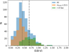 |
Fig. 14. Maximum host galaxy E(B−V) associated with each PN. In blue we show the full sample, in orange only the PNe brighter than 25.5 mag, and in green the PNe located within 4 kpc from the centre of the galaxy. The dotted line represents the median E(B−V) for the full sample, while the dashed-dotted line shows the median for PNe in the centre of the galaxy. |
5.4.2. Completeness
Another way the extinction could impact the PNLF is by affecting the completeness of the PNe sample, particularly in the dusty galaxy centre. Figure 15 shows how the number of PNe in concentric elliptical annuli changes as a function of distance from the centre of the galaxy both as an absolute measurement (top panel) and as the ratio of the number of PNe and the flux contained in the ellipse (bottom panel). To measure these quantities, we defined a series of ellipses centred on the centre of the galaxy and with constant PA and ellipticity and we counted how many PNe fell in each elliptical ring. We then used the WFI R-band image presented in Sect. 2.1.1 to extract the integrated flux in the same areas, masking bright stars, and we computed the ratio of the number of PNe and the flux contained in each annulus13. This quantity has been shown to be quite independent of the properties of the stellar population of a galaxy (Ciardullo et al. 1989; Buzzoni et al. 2006), and therefore, any variation might indicate changes in the PN sample completeness, perhaps due to dust extinction. Figure 15 shows that this quantity is relatively stable across the disk. Only rings with more that 50% coverage in our mosaic are included in the plot. At distances < 4 kpc however, the change in PNe/L is significant, which indicates a drop in the completeness. This happens both at the very centre, where we have the starburst ring and higher measured values of E(B−V), and around ∼3.5 kpc from the centre, which correspond approximately to the end of the bar. Figures 1 and 13 show strong dust lanes and high extinction values in these locations.
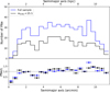 |
Fig. 15. Distribution of PNe as a function of distance from the centre of the galaxy. The top panel shows the number of PNe contained in concentric elliptical rings with growing semi-major axis. The bottom panel shows the luminosity-specific PNe number density measured in the same rings and normalised of its average value, since we are interested in the trend and not on its absolute value. We show the full sample in blue and the sample with m[OIII] < 25.5 mag in black. |
5.4.3. Modelling the extinction effects on the PNLF
In order to quantitatively assess the impact of dust extinction on the PNLF, we employ a straightforward model that describes the vertical distribution of dust and PNe within a disk to determine whether we could obtain a distance of 4.10 Mpc by applying extinction to samples of PNe extracted from the expected PNLF of a galaxy situated 3.5 Mpc away (27.72 mag), as is the case of NGC 253. Following the assumptions of Rekola et al. (2005), we consider that both PNe and dust are distributed following a Laplace distribution (also known as a double exponential distribution). This represents their vertical distribution across the galactic disk, where the maximum of the probability coincides with the disk plane. To keep the model simple, we assume a face-on disk, ignoring potential inclination effects. We first extract a sample of PNe from the PNLF and assign them a location within the disk by extracting it from their Laplace distribution. We then recover the expected extinction at their location from the cumulative distribution of dust normalised to the maximum extinction we considered. The extinction is then applied assuming a Cardelli et al. (1989) extinction law and an RV = 3.1. Finally, the modified PNLF was fitted with the method from Sect. 4.
We varied the maximum extinction from 0 to E(B−V) = 1 mag. Then, we set a fixed scale height for the PNe and examined multiple scale heights for the dust: half, one, two, four, and eight times the PNe scale height. For each combination of parameters, we repeated the entire process 50 times, considering the mean distance as our measurement and its standard deviation as our error. The results of this analysis are presented in Fig. 16. As expected, the extinction influences the distance inferred from the PNLF. Larger maximum extinctions result in more pronounced effects, making the galaxy appear further away, until a plateau is reached. Beyond this plateau, further increases in extinction do not affect the distance. The E(B−V) at which the plateau emerges depends on the relative scale heights of dust and PNe. When both are similarly distributed or when the dust has a higher scale height, we can recover our findings based on the anticipated PNLF of NGC 253. The E(B−V) at which this alignment occurs is approximately 0.3 mag if dust and PNe share the same scale height, consistent with Rekola et al. (2005). If the dust scale height exceeds that of the PNe, we need only and E(B−V) of 0.2 mag to explain our discrepancy. Finally, if the PNe scale height is larger than the dust one, the plateau is reached at very low E(B−V). In this case, the difference between the measured distance modulus and the expected one is small and cannot explain our discrepancy. This result is in line with the argument exposed by Feldmeier et al. (1997), which states that in this scenario there should always be a large enough number of bright and unextincted PNe to not affect the final distance.
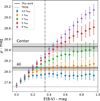 |
Fig. 16. Extinction effects on the distance modulus measured via the PNLF. The points show how the distance modulus estimated via a sample of PNe extracted from a PNLF with fixed zero-point and distance modulus (M* = −4.54 mag and 27.72 mag, respectively) changes when applying an increasing amount of extinction. In this model, both PNe and extinction (dust) follow a Laplace distribution, as described in Sect. 5.4. Different colours represent different ratios between the PNe and dust scale height. The solid horizontal lines represent our measurement of the distance modulus of the galaxy when considering both the full sample (bottom line) and only the PNe close to the centre of the galaxy (top line), while the grey areas represent their uncertainties. The dashed horizontal line represent a distance modulus of 27.72 mag, the expected one from the TRGB-based distances from the literature. Finally, the vertical dot-dashed line represents the average E(B−V) we measured from the extinction map shown in Fig. 13. |
Extinction can also explain the difference between the distances recovered from disk and the central PNLFs. In this case, Fig. 16 suggests that both a larger amount of extinction and a larger dust scale height are needed to explain our observations. In particular, it shows that the dust needs to be distributed with a scale height that is at least twice as large as the PNe one, while the maximum extinction needs to be ≳0.4, even though it changes significantly depending on the dust scale height.
This analysis suggests that internal extinction within the host galaxy is responsible for the discrepancies we observe, as well as for the differences in zero-point between the central and the disk PNLF. In particular, it suggests that in NGC 253 the dust is distributed with a similar scale height relative to the PNe in the disk, and a much larger scale height if we consider only the region close to the centre of the galaxy. This was not expected, since studies of both the Milky Way (Allen 1973; Li et al. 2018) and other edge-on nearby galaxies (e.g. Xilouris et al. 1999; Bianchi 2007; De Geyter et al. 2014) show how they exhibit a thin disk of dust, with a scale height half that of the stellar disk (where the PNe reside). In NGC 253 the starburst-driven outflow might be ejecting large quantities of dust-rich material from the centre of the galaxy, boosting the dust scale height. This effect is stronger close to the outflow, which is why we need a much larger scale height to explain the distance recovered from the central PNLF. The dust then settles when it moves further away from the outflow, but into a thicker disk with respect to more quiescentgalaxies.
The proximity of NGC 253 and availability of highly precise distance measurements from multiple techniques show how the assumption that the PNLF is independent of the amount of dust in a galaxy is not always correct. As stated by Jacoby et al. (2024), having large and heterogeneous galaxy samples with well-sampled PNLFs is essential to characterise the circumstances where the dust distribution significantly biases the PNLF distance. While correcting for the host galaxy dust extinction at any given position in the disk where a PN is found is challenging, our growing multi-wavelength views of the dust-rich ISM, along with the potential to develop rich kinematic models from the combined stellar and gas disk components, could be used to develop a statistical 3D approach to forward-model the line-of-sight dust extinction of the PNe population. Such an analysis is beyond the scope of this work but may present a novel way to refine the use of the PNLF as a rung in the cosmological distance ladder.
6. Summary and conclusions
We presented a new MUSE mosaic of the nearby starburst galaxy NGC 253. The mosaic includes 103 MUSE pointings and covers an approximate area of 20 × 5 armin2 with about nine million spectra, and it represents the largest mosaic of an extragalactic source ever observed by MUSE so far, except for the sparse mosaic of the Large Magellanic Cloud (Boyce et al. 2017). The data were observed as part of two ESO programmes (108.2289 and 0102.B-0078(A)) for a total of ∼53.5 h of observing time. The exposures were reduced using the official ESO MUSE pipeline (Weilbacher et al. 2020) through the pymusepipe wrapper (Emsellem et al. 2022) and were processed with the PHANGS data analysis pipeline, following the procedures described by Emsellem et al. (2022). Special care has been given to the sky subtraction because the redshift of the galaxy is low.
We then exploited moment-zero maps of the main emission lines ([O III]λ 5007, Hα, and [S II]λλ 6717,6731) to identify a sample of 571 PNe. We used 320 of them (those brighter than 25.5 mag, which was our estimated completeness limit) to build the PNLF of the galaxy and recover its distance. Following the procedure described by Scheuermann et al. (2022), we estimated a distance modulus of  mag (
mag ( Mpc), which is larger by ∼0.35 mag (0.6 Mpc) than expected from previous independent distance estimates based on PNLF fitting and the TRGB method. In particular, the TRGB-based distance (∼27.72 mag, 3.5 Mpc) was independently confirmed several times in the past 15 years and was proved to be a reliable reference. The PNLF analysis revealed the results we present below.
-
The distance recovered by Rekola et al. (2005) (
 mag or
  Mpc) was driven by the misclassification of their brightest region, which now appears to be an H II region. When this is removed from their sample, their distance agrees with ours.
 -
The zero-point of the relation changes significantly when only PNe located in the centre of the galaxy are considered, compared to those located in the outer disk. In particular, the inner PNLF returns a distance that is larger by ∼0.45 mag (0.9 Mpc) than the distance recovered from the remaining disk.
-
We reject metallicity as the origin of the discrepancy that we observe between our measurement and the literature. Preliminary measurement of the gas-phase metallicity and its gradient shows values corresponding to a negligible correction of the PNLF zero-point.
-
We also reject metallicity as the origin of the spatial variation in the PNLF because the observed behaviour would require an inverted metallicity gradient that is not observed in the galaxy.
-
A Balmer-decrement-based extinction map shows that the galaxy is affected by a significant amount of extinction. We estimated a median E(B−V) of ∼0.36 mag (A(V)∼1.1 mag), with peaks of > 6 mag (A(V) > 18 mag) close to the NGC 253 centre.
-
A simple model for the distribution of the PNe and dust showed that our results can be reproduced for the whole galaxy for a maximum E(B−V) ∼ 0.3 mag and the same scale height for dust and the PNe. The estimate from the central PNLF can be reproduced when the dust is distributed with at least twice the PNe scale height. This is in contrast to what is expected from scale-height studies of the Milky Way and other nearby edge-on galaxies (e.g. Allen 1973; Xilouris et al. 1999; Bianchi 2007; De Geyter et al. 2014), but it is compatible with a scenario in which the starburst-driven outflow enhances the vertical distribution of dust in NGC 253.
In conclusion, we showed that the PNLF is not a reliable method for estimating the distance of NGC 253 because its dust content is high and its distribution is peculiar. In general, it shows that dust should not be ignored in the PNLF analysis, especially for galaxies that are characterised by a high inclination and dust content. More galaxies with a well-sampled PNLF are required to characterise these effects better.
Data availability
The PNe catalogue is available at the CDS via https://cdsarc.cds.unistra.fr/viz-bin/cat/J/A+A/700/A125
Datacubes and selected products are available in the CADC (https://www.canfar.net/storage/vault/list/phangs/RELEASES/PHANGS-MUSE-NGC253) and ESO Phase 3 archive (https://doi.eso.org/10.18727/archive/100).
The absolute largest MUSE mosaic is that of the Large Magellanic Cloud and was published by Boyce et al. (2017). It covers 1 deg2 with a filling factor of 25%. Other large mosaics of Milky Way structures are available in the MUSE archive, although they have not yet been published.
skymethod=model in the scipost options.
We assume the aperture correction reported in Eq. (3) of Scheuermann et al. (2022).
On top of the abbreviations defined in the in the main text, in the figure we use the following abbreviations: BS for the brightest stars method, and Stat. for the statistical method.
Of the two missing objects the first is outside of our mosaic, while the second is not in our sample because of its extended morphology in the MUSE data.
Here we consider our original, best-estimate photometry.
The three points that significantly deviate from the relation at low distances represent very nearby dwarf galaxies: Pegasus, Leo A and WLM. Their PNLF-based distances are early attempts and are based on a very limited sample of PNe (one for Pegasus, one for Leo A and two for WLM; Jacoby & Lesser 1981). Therefore, we are not considering these three points in the analysis.
We assumed an average PSF FWHM of 0.8 across the mosaic (see Sect. 3.2) and we convolved it using a 2D Gaussian Kernel with the FWHM needed to recover a final FWHM of 5 arcsec. The spatial and spectral variation of the final FWHM is of the order of 0.1″.
Rekola et al. (2005) do not provide a model that we could test. Our analysis is based mainly on the discussion in their Sect. 3 and Fig. 4.
Since we are interested in the relative distribution of these points, and not in their absolute value, we did not convert the fluxes in luminosities.
Acknowledgments
The authors would like to thank our referee, Dr. Micheal Richer, for the excellent comments that helped improve this work. Based on observations collected at the European Organisation for Astronomical Research in the Southern Hemisphere under ESO programmes 108.2289 (PI: Congiu) and 0102.B-0078(A) (PI: Zschaechner). This work was carried out as part of the PHANGS collaboration. FS and KK acknowledge support from the Deutsche Forschungsgemeinschaft (DFG, German Research Foundation) in the form of an Emmy Noether Research Group (grant number KR4598/2-1, PI Kreckel) and the European Research Council’s starting grant ERC StG-101077573 (“ISM-METALS”). OE acknowledges funding from the Deutsche Forschungsgemeinschaft (DFG, German Research Foundation) – project-ID 541068876. E.C. and J.H. acknowledge the financial support from the visitor and mobility program of the Finnish Centre for Astronomy with ESO (FINCA). JEMD acknowledges support from project UNAM DGAPA-PAPIIT IG 101025, Mexico. A.D.B. and S.A.C. acknowledge support from the NSF under award AST-2108140. R.S.K. acknowledges financial support from the ERC via Synergy Grant “ECOGAL” (project ID 855130), from the German Excellence Strategy via the Heidelberg Cluster “STRUCTURES” (EXC 2181 – 390900948), and from the German Ministry for Economic Affairs and Climate Action in project “MAINN” (funding ID 50OO2206). RSK also thanks the 2024/25 Class of Radcliffe Fellows for highly interesting and stimulating discussions. This research has made use of the NASA/IPAC Extragalactic Database, which is funded by the National Aeronautics and Space Administration and operated by the California Institute of Technology. This research has made use of the Astrophysics Data System, funded by NASA under Cooperative Agreement 80NSSC21M00561. This research made use of Astropy, a community-developed core Python package for Astronomy (Astropy Collaboration 2013, 2018), Matplotlib (Hunter 2007), MPDAF (Bacon et al. 2016; Piqueras et al. 2017), NumPy (Harris et al. 2020), Photutils (Bradley et al. 2024), Pyneb (Luridiana et al. 2015), SciPy (Virtanen et al. 2020), Scikit-learn (Pedregosa et al. 2011).
References
- Acker, A., Marcout, J., Ochsenbein, F., et al. 1992, The Strasbourg-ESO Catalogue of Galactic Planetary Nebulae. Parts I, II (Garchingen: European Southern Observatory) [Google Scholar]
- Allen, C. W. 1973, Astrophysical Quantities (London: University of London, Athlone Press) [Google Scholar]
- Anand, G. S., Lee, J. C., Van Dyk, S. D., et al. 2021, MNRAS, 501, 3621 [Google Scholar]
- Anand, G. S., Tully, R. B., Cohen, Y., et al. 2024, ApJ, 973, 83 [Google Scholar]
- Arnaboldi, M., Aguerri, J. A. L., Napolitano, N. R., et al. 2002, AJ, 123, 760 [Google Scholar]
- Asplund, M., Grevesse, N., Sauval, A. J., & Scott, P. 2009, ARA&A, 47, 481 [NASA ADS] [CrossRef] [Google Scholar]
- Astropy Collaboration (Robitaille, T. P., et al.) 2013, A&A, 558, A33 [NASA ADS] [CrossRef] [EDP Sciences] [Google Scholar]
- Astropy Collaboration (Price-Whelan, A. M., et al.) 2018, AJ, 156, 123 [Google Scholar]
- Bacon, R., Piqueras, L., Conseil, S., Richard, J., & Shepherd, M. 2016, MPDAF: MUSE Python Data Analysis Framework, Astrophysics Source Code Library [record ascl:1611.003] [Google Scholar]
- Bailin, J., Bell, E. F., Chappell, S. N., Radburn-Smith, D. J., & de Jong, R. S. 2011, ApJ, 736, 24 [Google Scholar]
- Bates, D. R. 1946, MNRAS, 106, 509 [Google Scholar]
- Bauer, M., Pietsch, W., Trinchieri, G., et al. 2007, A&A, 467, 979 [NASA ADS] [CrossRef] [EDP Sciences] [Google Scholar]
- Beck, A., Lebouteiller, V., Madden, S. C., et al. 2022, A&A, 665, A85 [NASA ADS] [CrossRef] [EDP Sciences] [Google Scholar]
- Bendo, G. J., Beswick, R. J., D’Cruze, M. J., et al. 2015, MNRAS, 450, L80 [NASA ADS] [CrossRef] [Google Scholar]
- Bhattacharya, S., Arnaboldi, M., Gerhard, O., et al. 2021, A&A, 647, A130 [NASA ADS] [CrossRef] [EDP Sciences] [Google Scholar]
- Bianchi, S. 2007, A&A, 471, 765 [NASA ADS] [CrossRef] [EDP Sciences] [Google Scholar]
- Bolatto, A. D., Warren, S. R., Leroy, A. K., et al. 2013, Nature, 499, 450 [Google Scholar]
- Bottinelli, L., Gouguenheim, L., Paturel, G., & Teerikorpi, P. 1986, A&A, 156, 157 [NASA ADS] [Google Scholar]
- Boyce, H., Lützgendorf, N., van der Marel, R. P., et al. 2017, ApJ, 846, 14 [Google Scholar]
- Bradley, L., Sipocz, B., Robitaille, T., et al. 2024, https://doi.org/10.5281/zenodo.10671725 [Google Scholar]
- Bundy, K., Bershady, M. A., Law, D. R., et al. 2015, ApJ, 798, 7 [Google Scholar]
- Buzzoni, A., Arnaboldi, M., & Corradi, R. L. M. 2006, MNRAS, 368, 877 [Google Scholar]
- Cappellari, M. 2017, MNRAS, 466, 798 [Google Scholar]
- Cardelli, J. A., Clayton, G. C., & Mathis, J. S. 1989, ApJ, 345, 245 [Google Scholar]
- Ciardullo, R. 2010, PASA, 27, 149 [NASA ADS] [Google Scholar]
- Ciardullo, R. 2013, in Advancing the Physics of Cosmic Distances, ed. R. de Grijs, IAU Symp., 289, 247 [NASA ADS] [Google Scholar]
- Ciardullo, R., & Jacoby, G. H. 1999, ApJ, 515, 191 [Google Scholar]
- Ciardullo, R., Jacoby, G. H., Ford, H. C., & Neill, J. D. 1989, ApJ, 339, 53 [Google Scholar]
- Ciardullo, R., Feldmeier, J. J., Jacoby, G. H., et al. 2002, ApJ, 577, 31 [Google Scholar]
- Ciardullo, R., Durrell, P. R., Laychak, M. B., et al. 2004, ApJ, 614, 167 [Google Scholar]
- Cronin, S. A., Bolatto, A. D., Congiu, E., et al. 2025, ApJ, 987, 92 [Google Scholar]
- Croom, S. M., Lawrence, J. S., Bland-Hawthorn, J., et al. 2012, MNRAS, 421, 872 [NASA ADS] [Google Scholar]
- Dalcanton, J. J., Williams, B. F., Seth, A. C., et al. 2009, ApJS, 183, 67 [Google Scholar]
- Davidge, T. J., & Pritchet, C. J. 1990, AJ, 100, 102 [Google Scholar]
- Davidge, T. J., Le Fevre, O., & Clark, C. C. 1991, ApJ, 370, 559 [Google Scholar]
- Davis, B. D., Ciardullo, R., Jacoby, G. H., Feldmeier, J. J., & Indahl, B. L. 2018, ApJ, 863, 189 [Google Scholar]
- De Geyter, G., Baes, M., Camps, P., et al. 2014, MNRAS, 441, 869 [CrossRef] [Google Scholar]
- Della Bruna, L., Adamo, A., Bik, A., et al. 2020, A&A, 635, A134 [NASA ADS] [CrossRef] [EDP Sciences] [Google Scholar]
- Della Bruna, L., Adamo, A., Amram, P., et al. 2022, A&A, 660, A77 [NASA ADS] [CrossRef] [EDP Sciences] [Google Scholar]
- D’Odorico, S., Dopita, M. A., & Benvenuti, P. 1980, A&AS, 40, 67 [Google Scholar]
- Dopita, M. A., Jacoby, G. H., & Vassiliadis, E. 1992, ApJ, 389, 27 [Google Scholar]
- Draine, B. T. 2011, Physics of the Interstellar and Intergalactic Medium (Princeton University Press) [Google Scholar]
- Drory, N., Blanc, G. A., Kreckel, K., et al. 2024, AJ, 168, 198 [NASA ADS] [CrossRef] [Google Scholar]
- Emsellem, E., Schinnerer, E., Santoro, F., et al. 2022, A&A, 659, A191 [NASA ADS] [CrossRef] [EDP Sciences] [Google Scholar]
- Erroz-Ferrer, S., Carollo, C. M., den Brok, M., et al. 2019, MNRAS, 484, 5009 [Google Scholar]
- Feldmeier, J. J., Ciardullo, R., & Jacoby, G. H. 1997, ApJ, 479, 231 [NASA ADS] [CrossRef] [Google Scholar]
- Fitzpatrick, E. L. 1999, PASP, 111, 63 [Google Scholar]
- Gaia Collaboration (Brown, A. G. A., et al.) 2018, A&A, 616, A1 [NASA ADS] [CrossRef] [EDP Sciences] [Google Scholar]
- García-Rojas, J., Delgado-Inglada, G., García-Hernández, D. A., et al. 2018, MNRAS, 473, 4476 [CrossRef] [Google Scholar]
- Grasha, K., Chen, Q. H., Battisti, A. J., et al. 2022, ApJ, 929, 118 [NASA ADS] [CrossRef] [Google Scholar]
- Hanuschik, R. W. 2003, A&A, 407, 1157 [NASA ADS] [CrossRef] [EDP Sciences] [Google Scholar]
- Harris, C. R., Millman, K. J., van der Walt, S. J., et al. 2020, Nature, 585, 357 [NASA ADS] [CrossRef] [Google Scholar]
- Hartke, J., Arnaboldi, M., Longobardi, A., et al. 2017, A&A, 603, A104 [NASA ADS] [CrossRef] [EDP Sciences] [Google Scholar]
- Hartke, J., Arnaboldi, M., Gerhard, O., et al. 2020, A&A, 642, A46 [NASA ADS] [CrossRef] [EDP Sciences] [Google Scholar]
- Herrmann, K. A., Ciardullo, R., Feldmeier, J. J., & Vinciguerra, M. 2008, ApJ, 683, 630 [Google Scholar]
- Hlavacek-Larrondo, J., Carignan, C., Daigle, O., et al. 2011, MNRAS, 411, 71 [NASA ADS] [CrossRef] [Google Scholar]
- Hui, X., Ford, H. C., Ciardullo, R., & Jacoby, G. H. 1993, ApJ, 414, 463 [Google Scholar]
- Hunter, J. D. 2007, Comput. Sci. Eng., 9, 90 [NASA ADS] [CrossRef] [Google Scholar]
- Husemann, B., Jahnke, K., Sánchez, S. F., et al. 2013, A&A, 549, A87 [NASA ADS] [CrossRef] [EDP Sciences] [Google Scholar]
- Iodice, E., Arnaboldi, M., Rejkuba, M., et al. 2014, A&A, 567, A86 [NASA ADS] [CrossRef] [EDP Sciences] [Google Scholar]
- Jacobs, B. A., Rizzi, L., Tully, R. B., et al. 2009, AJ, 138, 332 [NASA ADS] [CrossRef] [Google Scholar]
- Jacoby, G. H. 1989, ApJ, 339, 39 [NASA ADS] [CrossRef] [Google Scholar]
- Jacoby, G. H., & De Marco, O. 2002, AJ, 123, 269 [Google Scholar]
- Jacoby, G. H., & Lesser, M. P. 1981, AJ, 86, 185 [Google Scholar]
- Jacoby, G. H., Ciardullo, R., Roth, M. M., Arnaboldi, M., & Weilbacher, P. M. 2024, ApJS, 271, 40 [Google Scholar]
- Jarrett, T. H., Cluver, M. E., Brown, M. J. I., et al. 2019, ApJS, 245, 25 [Google Scholar]
- Kippenhahn, R., Weigert, A., & Weiss, A. 2013, Stellar Structure and Evolution (Berlin, Heidelberg: Springer, Berlin Heidelberg) [Google Scholar]
- Kopsacheili, M., Zezas, A., & Leonidaki, I. 2020, MNRAS, 491, 889 [CrossRef] [Google Scholar]
- Krieger, N., Bolatto, A. D., Walter, F., et al. 2019, ApJ, 881, 43 [NASA ADS] [CrossRef] [Google Scholar]
- Leroy, A. K., Bolatto, A. D., Ostriker, E. C., et al. 2015, ApJ, 801, 25 [NASA ADS] [CrossRef] [Google Scholar]
- Leroy, A. K., Sandstrom, K. M., Lang, D., et al. 2019, ApJS, 244, 24 [Google Scholar]
- Leroy, A. K., Schinnerer, E., Hughes, A., et al. 2021, ApJS, 257, 43 [NASA ADS] [CrossRef] [Google Scholar]
- Li, L., Shen, S., Hou, J., et al. 2018, ApJ, 858, 75 [NASA ADS] [CrossRef] [Google Scholar]
- Li, J., Kreckel, K., Sarbadhicary, S., et al. 2024, A&A, 690, A161 [NASA ADS] [CrossRef] [EDP Sciences] [Google Scholar]
- Lindegren, L., Hernández, J., Bombrun, A., et al. 2018, A&A, 616, A2 [NASA ADS] [CrossRef] [EDP Sciences] [Google Scholar]
- Longobardi, A., Arnaboldi, M., Gerhard, O., et al. 2013, A&A, 558, A42 [NASA ADS] [CrossRef] [EDP Sciences] [Google Scholar]
- Lopez, S., Lopez, L. A., Nguyen, D. D., et al. 2023, ApJ, 942, 108 [NASA ADS] [CrossRef] [Google Scholar]
- Lucero, D. M., Carignan, C., Elson, E. C., et al. 2015, MNRAS, 450, 3935 [NASA ADS] [CrossRef] [Google Scholar]
- Luridiana, V., Morisset, C., & Shaw, R. A. 2015, A&A, 573, A42 [NASA ADS] [CrossRef] [EDP Sciences] [Google Scholar]
- Makarov, D., Prugniel, P., Terekhova, N., Courtois, H., & Vauglin, I. 2014, A&A, 570, A13 [NASA ADS] [CrossRef] [EDP Sciences] [Google Scholar]
- McCormick, A., Veilleux, S., & Rupke, D. S. N. 2013, ApJ, 774, 126 [NASA ADS] [CrossRef] [Google Scholar]
- McLeod, A. F., Ali, A. A., Chevance, M., et al. 2021, MNRAS, 508, 5425 [NASA ADS] [CrossRef] [Google Scholar]
- Moffat, A. F. J. 1969, A&A, 3, 455 [NASA ADS] [Google Scholar]
- Newman, M. J. B., McQuinn, K. B. W., Skillman, E. D., et al. 2024, ApJ, 966, 175 [Google Scholar]
- Nossal, S. M., Mierkiewicz, E. J., Roesler, F. L., et al. 2019, J. Geophys. Res. (Space Phys.), 124, 10,674 [Google Scholar]
- Okamoto, S., Ferguson, A. M. N., Arimoto, N., et al. 2024, ApJ, 967, L24 [Google Scholar]
- Osterbrock, D. E., & Ferland, G. J. 2006, Astrophysics of Gaseous Nebulae and Active Galactic Nuclei (University Science Books) [Google Scholar]
- Pedregosa, F., Varoquaux, G., Gramfort, A., et al. 2011, J. Mach. Learn. Res., 12, 2825 [Google Scholar]
- Piqueras, L., Conseil, S., Shepherd, M., et al. 2017, arXiv e-prints [arXiv:1710.03554] [Google Scholar]
- Radburn-Smith, D. J., de Jong, R. S., Seth, A. C., et al. 2011, ApJS, 195, 18 [Google Scholar]
- Reid, W. A., & Parker, Q. A. 2010, MNRAS, 405, 1349 [NASA ADS] [Google Scholar]
- Rekola, R., Richer, M. G., McCall, M. L., et al. 2005, MNRAS, 361, 330 [NASA ADS] [CrossRef] [Google Scholar]
- Rodríguez-González, A., Hernández-Martínez, L., Esquivel, A., et al. 2015, A&A, 575, A1 [NASA ADS] [CrossRef] [EDP Sciences] [Google Scholar]
- Roth, M. M., Jacoby, G. H., Ciardullo, R., et al. 2021, ApJ, 916, 21 [NASA ADS] [CrossRef] [Google Scholar]
- Rousseau-Nepton, L., Robert, C., Martin, R. P., Drissen, L., & Martin, T. 2018, MNRAS, 477, 4152 [NASA ADS] [Google Scholar]
- Rousseau-Nepton, L., Martin, R. P., Robert, C., et al. 2019, MNRAS, 489, 5530 [NASA ADS] [CrossRef] [Google Scholar]
- Sánchez, S. F., Kennicutt, R. C., Gil de Paz, A., et al. 2012, A&A, 538, A8 [Google Scholar]
- Scheuermann, F., Kreckel, K., Anand, G. S., et al. 2022, MNRAS, 511, 6087 [NASA ADS] [CrossRef] [Google Scholar]
- Schlafly, E. F., & Finkbeiner, D. P. 2011, ApJ, 737, 103 [Google Scholar]
- Schönberner, D., Jacob, R., Sandin, C., & Steffen, M. 2010, A&A, 523, A86 [NASA ADS] [CrossRef] [EDP Sciences] [Google Scholar]
- Solomon, S. C., Hays, P. B., & Abreu, V. J. 1988, J. Geophys. Res., 93, 9867 [Google Scholar]
- Stetson, P. B. 1987, PASP, 99, 191 [Google Scholar]
- Strickland, D. K., Heckman, T. M., Weaver, K. A., & Dahlem, M. 2000, AJ, 120, 2965 [NASA ADS] [CrossRef] [Google Scholar]
- Tully, R. B., & Fisher, J. R. 1977, A&A, 54, 661 [NASA ADS] [Google Scholar]
- Tully, R. B., & Fisher, J. R. 1988, Catalog of Nearby Galaxies (Cambridge University Press) [Google Scholar]
- Tully, R. B., Shaya, E. J., & Pierce, M. J. 1992, ApJS, 80, 479 [NASA ADS] [CrossRef] [Google Scholar]
- Tully, R. B., Rizzi, L., Shaya, E. J., et al. 2009, AJ, 138, 323 [NASA ADS] [CrossRef] [Google Scholar]
- Tully, R. B., Courtois, H. M., Dolphin, A. E., et al. 2013, AJ, 146, 86 [NASA ADS] [CrossRef] [Google Scholar]
- Vazdekis, A., Koleva, M., Ricciardelli, E., Röck, B., & Falcón-Barroso, J. 2016, MNRAS, 463, 3409 [Google Scholar]
- Virtanen, P., Gommers, R., Oliphant, T. E., et al. 2020, Nat. Methods, 17, 261 [Google Scholar]
- Wake, D. A., Bundy, K., Diamond-Stanic, A. M., et al. 2017, AJ, 154, 86 [Google Scholar]
- Walter, F., Bolatto, A. D., Leroy, A. K., et al. 2017, ApJ, 835, 265 [NASA ADS] [CrossRef] [Google Scholar]
- Weilbacher, P. M., Palsa, R., Streicher, O., et al. 2020, A&A, 641, A28 [NASA ADS] [CrossRef] [EDP Sciences] [Google Scholar]
- Westmoquette, M. S., Smith, L. J., & Gallagher, J. S. I. 2011, MNRAS, 414, 3719 [NASA ADS] [CrossRef] [Google Scholar]
- Willick, J. A., Courteau, S., Faber, S. M., et al. 1997, ApJS, 109, 333 [NASA ADS] [CrossRef] [Google Scholar]
- Xilouris, E. M., Byun, Y. I., Kylafis, N. D., Paleologou, E. V., & Papamastorakis, J. 1999, A&A, 344, 868 [NASA ADS] [Google Scholar]
- Yao, P. Z., & Quataert, E. 2023, ApJ, 957, 30 [Google Scholar]
Appendix A: DAOFIND based PNLF
In this section we repeat the selection of the PN candidates using the well-known point source detection algorithm DAOFIND (Stetson 1987). We apply the algorithm in the version included in the photutils package on the [O III]λ 5007 emission line map. We used default arguments for the detection and assume a PSF size of 1 arcsec. This detection approach returns a catalogue of 10635 PN candidates. We then processed the catalogue of PN candidates following the procedures described in Sec. 3 to measure the FHWM of each source, the line fluxes, and to remove contaminants from the sample. The final number of confirmed PNe is 5494, a rather high number compared to what identified in the emission line maps with the detection method described in Sec. 3.1. In fact, a visual inspection of the new candidates reveals that the vast majority of them are probably false detections. When we only consider sources with m[OIIII] ≤ 25.5 mag, however, the number decreases to 343, quite comparable to the 319 PNe that result from visual inspection. Matching the two catalogues, we see that 309 of the 320 confirmed PNe brighter than 25.5 mag are included in the clean sample of bright PNe from DAOFIND.
We used this clean sample of bright PNe to fit the PNLF (see Fig. A.1). As expected, given the similarity between the two samples, we obtain very similar results. In particular, we obtain a distance modulus of  mag, which corresponds to a distance of
  Mpc. Although the final results of the two detection methods are similar, the large number of false detections that are classified as PNe when using the DAOFIND catalogue made us decide to rely on visual identification for the main analysis of the paper.
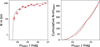 |
Fig. A.1. PNLF and cumulative luminosity function for NGC 253 using the sample of PNe recovered by DAOFIND. Panels, markers and colours as in Fig. 6. |
Appendix B: Additional tables.
Summary of the observations.
Summary of the information included in the PNe catalogue.
Wavelengths and ionisation potential of the relevant ion for each emission line.
List of FITS extensions included in the MAPS file
All Tables
Results of the K-sample Anderson-Darling test applied to each pair of sub-samples.
Wavelengths and ionisation potential of the relevant ion for each emission line.
All Figures
|
Fig. 1. Colour images of NGC 253 produced by combining broad-band images and emission-line maps extracted from the MUSE data cube. The mosaic covers an area of 20 × 5 arcmin2, and it includes roughly nine million independent spectra. The top panel shows a composition of three broad-band filters. The g band is plotted in blue, the r band in green, and the i band in red (Acknowledgement: ESO/M. Kornmesser). The bottom panel is a composition of emission line maps with [O III]λ 5007 in blue, Hα in green and [S II]λλ 6717,6731 in red. |
| In the text | |
|
Fig. 2. Hα region of the spectra in two different regions of the galaxy. The left panel represent the approaching side of the galaxy, and the right panel shows the receding side. In both panels we show in blue the spectrum extracted from the science exposure after our updated sky subtraction procedure, in orange the sky spectrum associated with the exposure, while the grey dashed lines represent the expected position of Hα at v = 0 km/s. |
| In the text | |
|
Fig. 3. Hβ region of the spectra in a circular aperture of 4 arcsec extracted from one of the pointings with an asymmetric Hβ profile. The blue line represents the spectrum obtained from the normal sky subtraction, while the orange line shows the spectrum obtained after removing the sky lines with wavelengths shorter than 5000 Å from the line list used to build the sky model from the dedicated sky offset. The vertical, dashed, grey line, represents the expected position of the Hβ emission line, considering the rotation curve of the galaxy. |
| In the text | |
|
Fig. 4. Example of the different images we used to visually detect nebulae. We show zoom-ins of four different areas of the galaxy. For each region, we show on the top the three colour map (same colours as in Fig. 1, bottom panel), in the middle the [O III]λ 5007 and in the bottom the Hα map. The circles highlight the position of nebulae in the final catalogue, with the solid circles showing the position of confirmed PNe and dotted ones showing nebulae classified either as supernova remnants or as compact H II regions. White triangles show the position of the objects identified by DAOFIND, which are, for the most part, spurious detections. |
| In the text | |
|
Fig. 5. [O III]λ 5007 line map of NGC 253. The empty circles mark the location of confirmed PNe. The dashed grey ellipses represent the boundary we used to define the radial bins presented in Sect. 5.2. |
| In the text | |
|
Fig. 6. PNLF and cumulative PNe [O III]λ 5007 luminosity function for NGC 253. The red points show the measured PNLF and cumulative function, and the dashed black line represents the best-fit model. The empty points mark the bins of the PNLF that were not considered in the fit. |
| In the text | |
|
Fig. 7. Comparison between the luminosity functions obtained from the three individual samples described in Sect. 3.1. The left panel shows the PNLFs, while the right panel shows the cumulative luminosity function. The figure shows how the three samples significantly overlap at the bright end, while the number of PNe drops in all cases around 25.5 mag. |
| In the text | |
|
Fig. 8. Comparison between our measurement (solid vertical black line) with errors (1σ, dark colour, and 3σ, lighter colour) with distances from the literature. All measurements are divided depending on the method used. Distances from: Bottinelli et al. (1986), Tully & Fisher (1988), Davidge & Pritchet (1990), Davidge et al. (1991), Tully et al. (1992), Willick et al. (1997), Rekola et al. (2005), Dalcanton et al. (2009), Jacobs et al. (2009), Tully et al. (2009), Radburn-Smith et al. (2011), Tully et al. (2013), Jacoby et al. (2024), Newman et al. (2024), Okamoto et al. (2024). |
| In the text | |
|
Fig. 9. Comparison between our PNe photometry and that of Rekola et al. (2005) and Jacoby et al. (2024). For Jacoby et al. (2024), we performed the comparison using both the data reduced by us, and the cubes directly recovered from the ESO archive. Solid symbols represent PNe that were used by the original authors in their PNLF computation. Open symbols represent objects that were not included in the final fit. |
| In the text | |
|
Fig. 10. Distance comparison for galaxies with PNLF and TRGB measurements from NED. The red points indicate galaxies where the PNLF was measured using imaging techniques, while blue points indicate PNLF measurements obtained with MUSE data. The grey line shows the one-to-one relation. The orange and light blue triangles identify the position of NGC 253 in the diagram when considering only imaging PNLF or MUSE-based PNLF, respectively. Error bars represent the range between the minimum and maximum values obtained via a specific method. We also annotated in the main panel the position of a few notable sources, and we plot Pegasus, Leo A, and WLM with open red circles. |
| In the text | |
|
Fig. 11. Effect of the aperture correction on the measured magnitude of the PNe in our sample. Only the objects brighter than 25.5 mag (vertical dashed line) have been used for the PNLF fit. We define Δ[OIII] as m(X × FWHM)−m(FWHM) with X being either 2 or 3. |
| In the text | |
|
Fig. 12. PNLF for the three PN subsamples at different galactocentric distances. The left column shows the PNLF and their fit, and the right column shows the cumulative luminosity function. The colours and symbols are the same as in Fig. 6. |
| In the text | |
|
Fig. 13. E(B−V) map of NGC 253. The E(B−V) was calculated from the Balmer decrement using a convolved (to a 5 arcsec FWHM Gaussian PSF) and binned version of the data in order to detect Hα and Hβ across most of the FOV. |
| In the text | |
|
Fig. 14. Maximum host galaxy E(B−V) associated with each PN. In blue we show the full sample, in orange only the PNe brighter than 25.5 mag, and in green the PNe located within 4 kpc from the centre of the galaxy. The dotted line represents the median E(B−V) for the full sample, while the dashed-dotted line shows the median for PNe in the centre of the galaxy. |
| In the text | |
|
Fig. 15. Distribution of PNe as a function of distance from the centre of the galaxy. The top panel shows the number of PNe contained in concentric elliptical rings with growing semi-major axis. The bottom panel shows the luminosity-specific PNe number density measured in the same rings and normalised of its average value, since we are interested in the trend and not on its absolute value. We show the full sample in blue and the sample with m[OIII] < 25.5 mag in black. |
| In the text | |
|
Fig. 16. Extinction effects on the distance modulus measured via the PNLF. The points show how the distance modulus estimated via a sample of PNe extracted from a PNLF with fixed zero-point and distance modulus (M* = −4.54 mag and 27.72 mag, respectively) changes when applying an increasing amount of extinction. In this model, both PNe and extinction (dust) follow a Laplace distribution, as described in Sect. 5.4. Different colours represent different ratios between the PNe and dust scale height. The solid horizontal lines represent our measurement of the distance modulus of the galaxy when considering both the full sample (bottom line) and only the PNe close to the centre of the galaxy (top line), while the grey areas represent their uncertainties. The dashed horizontal line represent a distance modulus of 27.72 mag, the expected one from the TRGB-based distances from the literature. Finally, the vertical dot-dashed line represents the average E(B−V) we measured from the extinction map shown in Fig. 13. |
| In the text | |
|
Fig. A.1. PNLF and cumulative luminosity function for NGC 253 using the sample of PNe recovered by DAOFIND. Panels, markers and colours as in Fig. 6. |
| In the text | |
Current usage metrics show cumulative count of Article Views (full-text article views including HTML views, PDF and ePub downloads, according to the available data) and Abstracts Views on Vision4Press platform.
Data correspond to usage on the plateform after 2015. The current usage metrics is available 48-96 hours after online publication and is updated daily on week days.
Initial download of the metrics may take a while.