| Issue |
A&A
Volume 700, August 2025
|
|
|---|---|---|
| Article Number | A199 | |
| Number of page(s) | 13 | |
| Section | Extragalactic astronomy | |
| DOI | https://doi.org/10.1051/0004-6361/202554939 | |
| Published online | 21 August 2025 | |
The undetectable fraction of core-collapse supernovae in luminous infrared galaxies
1
Tuorla Observatory, Department of Physics and Astronomy, University of Turku, 20014 Turku, Finland
2
School of Sciences, European University Cyprus, Diogenes Street, Engomi, 1516 Nicosia, Cyprus
3
School of Mathematical and Physical Sciences, Macquarie University, Sydney NSW 2109, Australia
4
Astrophysics and Space Technologies Research Centre, Macquarie University, Sydney NSW 2109, Australia
5
Cosmic Dawn Center (DAWN), University of Copenhagen, Jagtvej 128, 2200 København N, Denmark
6
Niels Bohr Institute, University of Copenhagen, Jagtvej 128, 2200 København N, Denmark
7
Finnish Centre for Astronomy with ESO (FINCA), University of Turku, 20014 Turku, Finland
8
South African Astronomical Observatory, P.O. Box 9, Observatory, 7935 Cape Town, South Africa
⋆ Corresponding author: This email address is being protected from spambots. You need JavaScript enabled to view it.
Received:
1
April
2025
Accepted:
20
June
2025
Abstract
Context. A large fraction of core-collapse supernovae (CCSNe) in luminous infrared galaxies (LIRGs) remain undetected due to extremely high line-of-sight host galaxy dust extinction and a strong contrast between the SN and the galaxy background in the central regions of LIRGs where the star formation is concentrated. This fraction of undetected CCSNe, unaccounted for by typical extinction corrections, is an important factor in determining CCSN rates, in particular at redshifts z ≳ 1, where LIRGs dominate the cosmic star formation.
Aims. Our aim is to derive a robust estimate for the undetected fraction of CCSNe in LIRGs in the local Universe. Our study is based on the K-band multi-epoch SUNBIRD survey dataset of a sample of eight LIRGs using the Gemini-North Telescope with the ALTAIR/NIRI laser guide star adaptive optics system.
Methods. We used simulated SNe and a standard image subtraction method to determine limiting detection magnitudes for the dataset. Subsequently, we used a Monte Carlo method to combine the limiting magnitudes with the survey cadence, and an adopted distribution of CCSN subtypes and their light curve evolution to determine SN detection probabilities. Lastly, we combined these probabilities with the intrinsic CCSN rates of the sample galaxies estimated based on their detailed radiative transfer modelling to derive the fraction of undetectable CCSNe in local LIRGs.
Results. For high angular resolution near-infrared surveys, we find an undetectable fraction of 66.0−14.6+8.6%, assuming that CCSNe with host extinctions up to AV = 16 mag are detectable, corresponding to the most obscured CCSN discovered in our dataset. Alternatively, assuming a host extinction limit of AV = 3 mag, corresponding to typical optical surveys, we find an undetectable CCSN fraction of 89.7−4.4+2.6%.
Key words: supernovae: general / dust, extinction / galaxies: star formation
© The Authors 2025
 Open Access article, published by EDP Sciences, under the terms of the Creative Commons Attribution License (https://creativecommons.org/licenses/by/4.0), which permits unrestricted use, distribution, and reproduction in any medium, provided the original work is properly cited.
This article is published in open access under the Subscribe to Open model. This email address is being protected from spambots. You need JavaScript enabled to view it. to support open access publication.
1. Introduction
Core-collapse supernovae (CCSNe) are the terminal explosions at the end of the lifetime of massive stars above ∼8 M⊙ (e.g., Smartt 2009). Due to the relatively short life cycles of massive stars (∼4 to ∼40 Myr), CCSNe trace the star formation rate (SFR). This offers an approach to estimate the SFR independently from the most commonly used galaxy luminosity-based methods. There is some disagreement about whether the observed CCSN rates match the theoretical CCSN rates based on SFR estimates. Horiuchi et al. (2011) suggests that up to z ≈ 0.4 the predicted CCSN rate is a factor of ∼2 higher than the observed CCSN rate. Cappellaro et al. (2015) agrees with this claim at 0.0 < z < 1.0, while Botticella et al. (2017) finds disagreements between the observed and the predicted CCSN rates at 0.15 < z < 0.35. The variety of methods of estimating SFRs might explain some of the disagreements (see e.g. Gruppioni et al. 2020). For example, Botticella et al. (2012) finds that their SFRs estimated from Hα and far-ultraviolet luminosities resulted in different CCSN rates between the two methods. Mattila et al. (2012) concludes that the likely reason for the discrepancy between the CCSN rate and SFR estimates is a large population of CCSNe that remain undetected due to extreme host extinctions. Their estimate for this additional missing fraction of CCSNe ranges from 19% at z = 0 to 38% at z ≈ 1.2. Melinder et al. (2012) and Dahlen et al. (2012) use the results of Mattila et al. (2012) to correct for the effects of the missing fraction, and find that the theoretical and observed CCSN rates match within the errors at 0.1 < z < 1.0 and 0.4 < z < 1.0, respectively. However, the results of Strolger et al. (2015) suggest that the observed and expected CCSN rates are in a reasonable agreement at 0.1 < z < 2.5.
Luminous infrared galaxies (LIRGs) and ultraluminous infrared galaxies (ULIRGs) are defined as galaxies with 1011 L⊙ < LIR < 1012 L⊙ and 1012 L⊙ < LIR < 1013 L⊙, respectively, which have enhanced SFRs (e.g. IC 883 with a high SFR of roughly 233 M⊙ yr−1; Kankare et al. 2021). The source of the high infrared luminosity can be an active galactic nucleus (AGN), star formation, or both. They often show signs of past interaction, or are actively merging. The primary source of LIR in LIRGs with enhanced SFRs is the reprocessing of light from young hot stars via dust and gas (Kennicutt 1998; Pérez-Torres et al. 2021). Since the star formation in LIRGs is concentrated in the nuclear and circumnuclear regions at scales of ∼0.1 to ∼1 kpc (Soifer et al. 2001), a considerable fraction of SNe are not discovered due to extinction and insufficient spatial resolution of the observations (Kool et al. 2018). The differences between the observed and predicted CCSN rates are likely to only increase at higher redshifts, where LIRGs start to dominate star formation, with increasing contributions as redshift increases (Le Floc’h et al. 2005; Magnelli et al. 2011). At z = 1 the contribution of LIRGs is ∼50% to the SFR (e.g. Magnelli et al. 2009).
Core-collapse supernova rate studies typically correct their observed rates with extinction correction models (e.g. Riello & Patat 2005). However, a fraction of CCSNe can have very high localised extinctions that these extinction correction models do not take sufficiently into account. This population of CCSNe with extreme host extinctions that remain undiscoverable, and unaccounted for after CCSN rate extinction corrections, results in an additional fraction of CCSNe that are missed by surveys, hereafter referred to as the missing fraction. Furthermore, we use the term undetectable fraction to refer to the combined fraction of SNe that would remain undiscovered due to belonging either to the population with sufficiently high host extinctions described by the extinction correction model or to the population described by the missing fraction.
Mattila et al. (2012) estimate that as much as  of CCSNe in LIRGs are missed by optical surveys due to extreme host extinctions. This estimate is based on a number of CCSNe found in one nearby LIRG system (Arp 299) by several surveys over 14 years. Miluzio et al. (2013) find that in ground-based seeing K-band observations, where the extinction is ∼10% of the optical extinction, the percentage of CCSNe missed in LIRGs can be as high as ∼60% to 75%. Their estimate is based on artificial star experiments on their sample galaxies. This is in general agreement with a previous result by Mannucci et al. (2007), which estimates that ∼30% of CCSNe are missed at z ≈ 1, since 50% of SFR is in LIRGs at that redshift. A survey with the Spitzer Space Telescope at 3.6 μm by Fox et al. (2021) monitored a sample of (U)LIRGs for 2 years, and detected 9 CCSNe out of the expected intrinsic number of 51.9 CCSNe in the 32 (U)LIRGs at < 150 Mpc within which the survey was found to be sufficiently sensitive; this suggests that ∼83% of CCSNe remained undetected.
An excellent alternative to space-based surveys are monitoring observations with adaptive optics (AO) at near-IR wavelengths from 8 metre-class ground-based telescopes, as shown by multiple CCSN discoveries in LIRGs (Mattila et al. 2007; Kankare et al. 2008, 2012; Kool et al. 2018). The distribution of all optical or infrared detected CCSNe in LIRGs is presented by Kool et al. (2018, see their Figure 11) with the projected nuclear offsets and discovery methods reported. While optical surveys find most of the CCSNe in the sample at nuclear distances of > 4 kpc, non-AO and AO NIR surveys dominate closer to the nucleus when taking into account the smaller sample size. The data also suggests that performing a survey in less dust-obscured NIR bands alone is not enough due to the poorer spatial resolution of non-AO NIR surveys compared to the high-resolution methods, and a combination of AO and NIR bands are required to effectively detect CCSNe in the nuclear regions of LIRGs. Therefore, the usage of near-IR bands compared to optical bands has the most important influence on the detectability of obscured CCSNe in LIRGs, with the high-resolution methods providing a crucial addition for the surveys. Thus, accurate estimates for the percentage of CCSNe that remain undetected by CCSN rate surveys can be estimated with improved accuracy using this high-resolution method.
Deep IR observations with the James Webb Space Telescope (JWST) have recently started producing CCSN discoveries at redshifts beyond z = 3 (DeCoursey et al. 2025) whereas Euclid and Roman Space Telescope will be increasing substantially the CCSN rate statistics at z ≳ 1. Reliable corrections for the CCSNe remaining undetected by these surveys due to very high extinctions in dusty galaxies across the redshift (e.g. Mattila et al. 2012) will allow detailed comparisons with the rates expected from the cosmic SFRs.
Core-collapse supernovae are classically divided into subtypes based on their light curves and spectral features (Filippenko 1997). This work considers CCSN subtypes II, IIn, IIb, Ib, Ic, and SN 1987A-like. Type IIb, Ib, and Ic are called stripped envelope SNe and exhibit spectral features indicative of increased envelope stripping, respectively showing some hydrogen, helium but no hydrogen, and neither hydrogen nor helium. Type II refers to hydrogen-rich SNe, which are sometimes further classified to Type II-P and II-L based on their light curve evolution. Type IIn SNe are hydrogen-rich, but exhibit narrow spectral lines (≲1000 km s−1). Finally, SN 1987A-like events are peculiar hydrogen-rich CCSNe that resemble SN 1987A with a slowly rising optical light curve.
Our method of analysing the data (Sect. 2) was the following. Algorithmic image subtraction (Sect. 3.1) was used as a method to detect SNe in the dataset. The limiting magnitudes (Sect. 3.2) were determined for CCSN detections via injection of artificial SNe and automated detection of these sources. Subsequently, a Monte Carlo method (Sect. 3.3) was used for collating effects of different CCSN subtypes, peak magnitude variation, evolution timescale variability of CCSNe, host extinction, and observational cadence to produce CCSN detection probabilities for the dataset. The intrinsic CCSN rates were estimated for the dataset using modelling of the spectral energy distribution (SED) of the sample LIRGs, where radiative transfer models for different components of the galaxy were fitted to the SEDs. The intrinsic CCSN rates were then compared with the observed rates to derive the missing fraction estimate, and the adopted host extinction model was used to derive the survey depth dependent fraction of CCSNe that would remain undiscovered. These two effects were combined to derive the total undetectable fraction of CCSNe in LIRGs, and is reported in Sect. 4. Conclusions are provided in Sect. 5.
2. Dataset
The dataset analysed in this study was obtained by the Supernovae UNmasked By Infra-Red Detection (SUNBIRD) collaboration (Kool et al. 2018) with the aim to discover and study CCSNe in high-SFR LIRGs. The data consists of 67 epochs of eight different LIRGs in total, spanning from March 2007 to August 2012, see Table 1. The data were obtained using the Gemini-North Telescope with the Near-InfraRed Imager (NIRI; Hodapp et al. 2003) and the ALTtitude conjugate Adaptive optics for the InfraRed (ALTAIR) laser guide star AO system (0.022″ pixel−1) in K-band. The total on-source exposure times of the analysed images were typically 9 × 30 s; however, in a few cases the number of co-adds varied from a minimum of four to a maximum of 18. Each 30 s image was obtained in individual exposures of one to ten seconds depending on the brightness of the galaxy nucleus. No separate frames were taken for sky background subtraction, instead the sky images were created from the dithered 30 s images of the target. The data reduction was carried out with the external gemini package in Image Reduction and Analysis Facility (IRAF, Tody 1986) to perform the typical steps of flat field correction, sky subtraction, and co-addition of the processed images. For each galaxy, all the ALTAIR/NIRI images were aligned to match the epoch with the best seeing using the IRAF tasks geomap and geotran.
Summary of the dataset.
The photometric calibration was based on the Two Micron All Sky Survey (2MASS; Skrutskie et al. 2006). Due to the small 22″ × 22″ field of view (FOV) of the ALTAIR/NIRI setup, there were no isolated 2MASS point sources in the target frames. Magnitudes of bootstrapped sequence stars in the fields were adopted for IRAS 17138−1017, IC 883, Arp 299-A, and Arp 299-B from the analyses of Kankare et al. (2008, 2012, 2014), previously obtained for the studies of CCSNe discovered in these LIRGs. For the calibration of the images of the other LIRGs, we made use of Ks-band images of the galaxy fields obtained using the Nordic Optical Telescope (NOT; Djupvik & Andersen 2010) with the NOT near-infrared Camera and spectrograph (NOTCam) instrument. The NOTCam images were reduced using the external notcam package in IRAF, which included flat field correction, sky subtraction, and co-adding individual frames for higher signal-to-noise ratio. With the NOTCam FOV of 4′×4′ typically several 2MASS point sources were found in the reduced images to calibrate their zeropoints. Subsequently, common point sources in both the NOTCam and the ALTAIR/NIRI images were identified and their magnitudes were measured to use them for the calibration of the ALTAIR/NIRI data of IRAS 16516−0948 and IRAS 17578−0400. The aperture photometry was carried out using the Source Extractor program (Bertin & Arnouts 1996). In the case of two galaxies, CGCG 049−057 and MCG+08-11-002, there were no point sources in the ALTAIR/NIRI images. In these cases the whole galaxy was measured with a largest possible aperture for the ALTAIR/NIRI images, and calibrated accordingly with an identical aperture using the NOTCam images. In these two galaxies the aperture photometry was performed with IRAF due to the poor performance of Source Extractor with extended objects.
The point spread function (PSF) of the AO images includes a narrow core and extended wings. The exact sizes of these and the Strehl ratio depends on observational conditions, for example seeing, brightness of the natural guide star and its distance from the target. In our dataset, the median measured full width at half maximum (FWHM) of the PSF core was six pixels (corresponding to 0.13″), the standard deviation was 3.1 pixels, and the 95th percentile was at 9.4 pixels. Performing aperture photometry with conventional aperture sizes can miss a significant portion of the flux from the extended wings. We measured the effect of this by performing aperture photometry on a field star from an AO image with a progressively larger aperture until the measured brightness of the star remained constant. The resulting aperture correction was the difference between this end magnitude and the magnitude at the aperture size used in the photometry. The bootstrapped magnitudes from the NOTCam images were then corrected by this aperture correction.
Five CCSNe have been previously reported based on the ALTAIR/NIRI dataset: SN 2010cu (Type IIP, AVhost = 0 mag) and SN 2011hi (Type IIP, AVhost = 6 mag) in IC 883 (Kankare et al. 2012), SN 2010O (Type Ib, AVhost = 1.9 mag) and SN 2010P (Type IIb, AVhost = 7 mag) in Arp 299-A/B (Kankare et al. 2014), and SN 2008cs (Type IIn, AVhost = 16 mag) in IRAS 17138−1017 (Kankare et al. 2008). No new previously unreported CCSN candidates were discovered in the dataset during our analysis. The discovered number of CCSNe was compared to the expected number of events in our analysis.
3. Method
We begin by summarising the overall method. First, we developed an automated process for the template subtraction of the survey images, which was carried out for the dataset. Second, we derived spatially variable limiting magnitudes for each epoch of each galaxy. Third, we derived detection probabilities of individual simulated SNe for each galaxy in the dataset via a Monte Carlo simulation. Finally, the detection probabilities were combined with intrinsic CCSN rates estimated with radiative transfer modelling of the SEDs of the sample galaxies to derive the missing fraction of CCSNe in LIRGs. The undetectable fractions of CCSNe were derived combining the results from the host extinction model and missing fraction estimate. Details of these individual steps are provided in the following subsections.
3.1. Automatic image subtraction
We used the method described by James & Anderson (2006) to create galaxy region maps for each of the sample LIRGs in the ALTAIR/NIRI data. First, we created a median stacked image for every sample galaxy, where each pixel value is the median value of that pixel from all the aligned epochs of the images. Then a background level was subtracted from the median image. This background level was selected as an area far from the galaxy and field stars. Finally, the pixel values were summed from the lowest to the highest. The ranked pixels are considered to be part of the background until the sum reaches zero, and the not yet included pixels belong to the galaxy. Regions of a few hundred pixels in width at the edges of the images with a lower signal-to-noise ratio were excluded from the process. Field stars were manually removed from the galaxy maps. An example of a median stacked image and the corresponding galaxy map is shown in Fig. 1. The exact location of the background sample area does have some effect on the galaxy maps (i.e. in the extent of the outer edges of the galaxy). However, the effect of this on our method is minimal, since the expected CCSN rate at the outer edges of the galaxy is low.
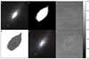 |
Fig. 1. Galaxy IC 883 in different stages of determining the limiting magnitudes. (a) 22″ × 22″ median stacked image of the sample galaxy IC 883. (b) Galaxy map constructed from the median stacked image. (c) Example of a template subtraction. (d) Limiting magnitudes of IC 883 with the scale on the right. The two white pixels in the centre of the galaxy represent areas where persistent template subtraction artefacts prevented analysis; further details are provided in Sect. 3.2. (e) Example stamp positions for four sets of stamp lists. The red squares denote the non-varied stamps in the stamp lists and the blue squares denote the varied stamp. The positions of both sets was changed in a subsequent run to ensure that the whole galaxy was covered. (f) Example of the limiting magnitude iteration process. Visible point sources are simulated SNe at 16.8 mag, which are positioned on the galaxy map, excluding the stamp areas, separated by 7 × FWHM = 42 pixels. |
Image subtraction is a basic method used by SN search programs. Sources in an image that remain constant between epochs (e.g. stars and galaxies) disappear in a good quality subtraction. Conversely, transient sources (e.g. sufficiently bright CCSNe) remain detectable in the subtracted image if the source brightness has evolved sufficiently between the epochs or the source is not present in one of the images. However, in practice, the image subtraction methods can leave residuals in the subtracted image, in particular to the brightest regions of the field. Furthermore, the noise in the image is increased by a factor of  in the process. The optimised subtraction parameters were obtained for each image in the dataset. For each image the subtraction template image was selected based on having the most similar image quality and at least 200 days difference in time between the epochs of the images.
The image subtraction process in our analysis was carried out using a slightly modified version of the ISIS2.2 package (Alard & Lupton 1998; Alard 2000). The user provides the software two aligned images, with a similar PSF for best results, and enables the software to select stamp regions automatically or provides them externally for the code. These stamps consist of two co-centric squares with inner and outer areas. The inner areas are used to generate a convolution kernel to convolve the image with the narrower PSF to match the image with the broader PSF. The outer area is used to measure the background of the image. After calculating the convolution kernel, the software performs the image convolution, scales the fluxes to match, and subtracts the images pixel by pixel. The quality of the image subtraction result is highly dependent on some of the adopted parameters (e.g. Melinder et al. 2012). In order to reduce the subjective bias in this process, we developed an automatic algorithm to optimise the parameter selection.
Our algorithm optimises three key image subtraction parameters for ISIS2.2, assuming that they are largely independent: the kernel size, the size of the background fit region, and the degree of the kernel fit. The degree of the kernel fit dictates how much the kernel is allowed to vary across the image. Too high of a degree compared to the number of stamps provided can cause overfitting. The algorithm starts with a set of initial guesses for the values for kernel and stamp size provided by the user. The program then performs a subtraction using all the combinations of the initial guesses. It then chooses the best combination of the kernel and stamp sizes. The quality of the subtraction is measured as the variance of pixel values across the area included in the galaxy map, excluding the stamp regions. A new set of values for the parameters are then generated above and below the previously selected best values. The program then performs subtractions using all the combinations of these new values, and again chooses the best ones. This iterative process continues until no improvements are made anymore, or the upper or lower bounds of the parameters set by the user are reached. One caveat of this approach would be that it might converge to some local minima, and miss the optimal parameter values. However, according to our tests, the quality of the subtraction evolves smoothly as a function of these variables, and thus this is not a major concern. After kernel and stamp sizes are set, the algorithm tests which degree of kernel variation is optimal.
Furthermore, our algorithm varies the selection of the used stamps from an initial list provided by the user (see Fig. 1). If a SN occurs within a stamp location used to derive the convolution kernel by the image subtraction package, the SN might disappear or become fainter in the process. ISIS2.2 includes an automatic step that should reject such stamps; however, this is uncertain if the SN is faint compared to the surrounding pixels and close to the detection threshold. Therefore, the algorithm is given two sets of stamps: one set that is fixed during a run and a second set which is varied during the optimisation process. The results of the process are two lists of optimal stamp locations and corresponding image subtraction parameter values, where the varied stamp locations do not overlap between the two lists. In an optimal scenario two varied stamp lists is enough to cover the entire galaxy; however, in most cases one to two additional varied stamp lists are required to ensure high-quality subtractions over the whole galaxy when the results are combined. An example subtraction is shown in Fig. 1.
3.2. Limiting magnitudes
Noise in the subtracted images and image subtraction residuals affect the detection probabilities of SNe. To take this into account, we developed a program to simulate artificial SNe in sequences of different magnitudes on the ALTAIR/NIRI images with the aim to recover them after the image subtraction process to derive the detection thresholds. This results in spatially variable limiting magnitudes for each epoch. An example of a final product of this method is shown in Fig. 1.
The artificial SNe were created with the IRAF routine mkobjects. Simulated SNe have a Moffat profile with a Moffat parameter of 2.5, which is typical for seeing limited profiles, and a seeing value that matches the FWHM of the narrow core PSF of point sources in the analysed image. This approach was chosen since most of the sample galaxies in the ALTAIR/NIRI data did not have bright point sources in the FOV and two of the LIRGs (MCG+08-11-002 and CGCG 049-057) did not have any point sources from which to determine an accurate description of the full AO PSF including the faint and extended wings. Thus for consistency across the dataset we used the Moffat profile for the whole dataset. In order to estimate the effect of this, we repeated the limiting magnitude procedure for the LIRG IRAS 17578−0400 with the usage of a PSF of a bright star in the FOV (including the AO PSF wings) instead of the Moffat profile. The resulting limiting magnitude differences from those with the Moffat profile were on average less than the 0.2 mag step used to derive the detection threshold. Therefore, the usage of the Moffat profile to describe the dominant narrow PSF core seems sufficient for our analysis.
The SNe are simulated on the pixels based on the galaxy map; however, limited to a grid size that corresponds to the FWHM of the narrow PSF core of point sources in the image. For example, for a typical image with a FWHM ≈ 5 pixels, the artificial SNe are simulated on the galaxy map covered area in a grid where the sources are separated by 5 pixels in both the x and y directions. However, if all these artificial SNe would be created in the image simultaneously, their detection as individual sources would be impossible due to the blending of the sources; therefore, the complete grid of simulated SNe has to be divided into subgrid parts. Based on our tests, a separation of 7 times the image FWHM between each SN was sufficient to prevent any notable overlap effects. Therefore, the initial grid is divided into 64 subgrids where the artificial SNe are separated by ≥7 × FWHM. An example of a subgrid is presented in Fig. 1.
An iterative process was then carried out for these 64 subgrids consecutively. The automatic process consisted of creating artificial SNe with IRAF, carrying out the image subtraction with ISIS2.2, detecting the SNe with Source Extractor, and iterating the process making the SNe fainter until none are detected. Areas within 10 × FWHM of known real SNe were excluded from the analysis in epochs where the events were detectable. This was done to avoid any pre-existing SN from affecting the detection of nearby simulated SNe. We note that the probability of two simultaneous SNe with overlapping locations is extremely low and the excluded regions were small.
Simulated SNe were detected from the subtracted images using Source Extractor with the following parameters: minimum pixel area of 9 and a detection threshold of 5σ above background. The minimum pixel area was chosen to strike a balance between weeding out most image subtraction artefacts, while having a minimal effect on the detection of dim artificial SNe. The 5σ level was chosen conservatively, and result in a threshold where the SNe are sufficiently distinguishable by eye. Occasionally noise effects shifted the location of the simulated SNe approximated by Source Extractor in the subtracted image. To prevent this effect from causing false non-detections, a simulated SN was counted as a detection if a source was detected within four pixels of a simulated SN position. The range of four pixels was found by testing to be sufficient, while not causing false positives. Since Source Extractor does not perform PSF fitting of the sources, it is more challenging to avoid identifying artefacts as detections compared to PSF fitting-based methods. These false detections were confirmed to be artefacts rather than real detections by inspecting their light profiles. Their profiles were unnaturally narrow and asymmetric to be real detections. The locations with an artefact in the subtracted image were not analysed with simulated SNe. The effect of these artefacts was mitigated by performing multiple sets of image subtractions; however, in some unfortunate cases artefacts can appear in the same locations of subtracted images also with different sets of selected stamps. In these few cases those grid points are conservatively considered as non-detectable for the purpose of the analysis.
The iterative process to determine the detection threshold magnitudes was the following. Initially, a subgrid set of artificial SNe with an apparent magnitude of 16 mag were simulated on the image to be analysed. This was considered as a conservative starting magnitude for the simulated sources, which would be clearly detectable in a vast majority of the image subtracted pixels. The image subtraction was then carried out with the optimal parameters and stamp selections determined by the algorithm, and the resulting artificial SN detections were recorded. Subsequently, the process was repeated with simulated SNe that were 0.2 mag fainter than before, until either all SNe result in non-detections, or 40 iterations have been carried out. Following this, another spatially shifted subgrid of SN positions was analysed, and the process continued until the full set of 64 subgrids is complete. Finally, if there were any simulated SNe that were undetected at 16 mag, the complete process was repeated for those locations starting at 14 mag. The 14 mag limit for the brightest simulated SNe was chosen to roughly match the brightest expected CCSNe in the nearest galaxy of the dataset. For those artificial SN positions that had a detection threshold magnitude determined more than once in a set of stamp lists, the faintest magnitude was chosen as the threshold. The limiting magnitudes were determined for each epoch in the dataset, and each pixel in the galaxy maps. If the two epochs used in the subtraction had very similar FWHM values, the same detection limits were adopted for the two images.
3.3. Monte Carlo method
Miluzio et al. (2013) used a Monte Carlo method to estimate SN detection probabilities in their dataset. This involved simulating SNe in different regions of their galaxy sample, with varying luminosities and using K-band light curve models for the different SN subtypes. Depending on the explosion dates, extinction parameters and limiting magnitudes, the individual SNe were counted as either detections or missed events. Our approach is similar to their work, with the focus on AO searches for CCSNe in LIRGs extending over more years.
The individual components required for the method were the following: detection thresholds for the faintest detectable SNe in each pixel in each epoch of the dataset, templates for the light curve evolution for each CCSN subtype and limits within which they vary, a model for the host extinction, the survey cadence, the adopted relative rates of CCSN subtypes, and finally the intrinsic total CCSN rates for the dataset. Each run of the Monte Carlo program simulated 107 SNe. The following procedure was used. Time resolution for the simulation was set to one day and spatial resolution to one pixel in the galaxy maps. First a CCSN subtype is chosen, then a random day is chosen within the typical detection window (i.e. control time, see Sect. 3.3.3) for that subtype of chosen galaxy as the explosion date. Then a pixel in the galaxy map was randomly chosen as the SN location based on the probability to host a CCSN. This probability was assumed to be directly proportional to the ratio of the flux within a radius of five pixels around that position and the total flux of the LIRG in K-band. The total flux was the measured sum of the pixel values within the galaxy map area in the median stack of all epochs of the galaxy. Next the CCSN subtype template light curve was generated, and its absolute brightness was determined based on the time to the next observation epoch. Finally the distance modulus was added to the absolute magnitude and the galactic and host extinction effects were included. The resulting SN apparent magnitude was then compared against the limiting magnitude of that pixel in the epoch where the SN would be first observable. If the SN was brighter than the limit, it was counted as a detection.
3.3.1. Template light curves
Core-collapse supernova subtypes included in the simulation were: II, IIn, IIb, Ib, Ic, and SN 1987A-like. The relative rates of these CCSN subtypes were adopted from the observed volume-limited results of the Lick Observatory Supernova Search (LOSS, Li et al. 2000) with CCSN classifications revised by Shivvers et al. (2017). Our work adopted the CCSN magnitudes and their revised subtypes with small modifications; we did not separate Type II SNe into subtypes Type II-P and II-L, as there is some evidence of them being the same population (e.g. Anderson et al. 2014), the relative rates of Type IIb-peculiar SNe were merged with the Type IIb SNe, and both Type Ic-peculiar and broad-line Type Ic SNe were included in the Type Ic SN fraction. This is justified by the low rates combined with the lack of high-quality K-band light curves for these rare subtypes. Type Ia SNe were not considered in the analysis due to their low relative rates (∼5%) compared to CCSNe in high SFR galaxies (see e.g. Mattila et al. 2007). These relative rates assume identical explosion time windows for the CCSNe, which is not the case in the Monte Carlo simulation. The relative rates were slightly adjusted for each galaxy to counteract this effect. For example, if one CCSN subtype has double the time window to explode compared to the rest, its relative rate needs to be doubled so that the number of CCSNe per year for that subtype stays constant.
Requirements for the K-band SN light curve datasets from the literature to be adopted as templates were the following: smooth evolution with small photometric errors and an adequate cadence, early photometric points to sufficiently cover the light curve rise and peak, and a sufficient late-time coverage. Furthermore, the explosion date of the SN was required to be well constrained. This resulted in only a few candidates for each subtype. Thus, it was opted to adopt for each subtype only the most representative high-quality light curve as the template. Due to the similar K-band light curve evolution of the stripped-envelope SNe (types IIb, Ib, Ic) these were represented by the well observed Type IIb SN 2011dh (Ergon et al. 2014, 2015). For the Type II template light curve SN 1999em was chosen (Krisciunas et al. 2009). For the Type IIn template light curve SN 1998S was chosen (Fassia et al. 2000; Pozzo et al. 2004). For the SN 87A-like light curve SN 1987A was chosen (Bouchet et al. 1989; Bouchet & Danziger 1993). For these subtypes and the selected template SNe relevant information is listed in Table 2.
Template light curve parameters.
The unfiltered peak absolute magnitude distributions for each SN subtype were obtained from the sample of Li et al. (2011), corrected with the updated SN classifications by Shivvers et al. (2017). Only CCSNe with unambiguous classifications were included. Since the data by Li et al. (2011) does not include any estimates or corrections for the host galaxy extinction, we limited the sample selection to SNe with host inclinations of < 75° to reduce the effect of the extinction in our absolute magnitude distributions by excluding the most edge-on galaxies. This reduced the number of CCSNe used for these distributions from 88 to 69. The peak absolute magnitude distributions of Li et al. (2011) were obtained without a filter, which is best approximated by R-band.
We examined CCSN light curves from the literature and measured their R − K colours at both the R and K-band light curve peaks, see Table 2. We limited our peak colour sample to CCSNe with the same criteria as used for the template light curves, which resulted in four H-poor SNe and four Type II SNe. For Types IIn and SN 87A-like we used only the model SNe themselves due to the poor availability of high quality light curves. For SN 1998S we adopted a more recent extinction estimate by Shivvers et al. (2015) of AV = 0.16 mag, as opposed to the value of AV = 0.68 mag by Fassia et al. (2000). The four H-poor SNe included here were: SN 2002ap (Borisov et al. 2002), SN 2007gr, SN 2009jf (Bianco et al. 2014), and SN 2011dh (Ergon et al. 2014, 2015). The four Type II SNe included were: SN 1999em (Krisciunas et al. 2009), SN 2007aa, SN 2008in (Hicken et al. 2017), and SN 2013ej (Yuan et al. 2016). We applied the yielded colour values to the unfiltered absolute peak magnitude distributions to obtain K-band absolute peak magnitude distributions. An alternative approach would have been to derive peak magnitude statistics directly from the K-band light curves from the literature, which we deemed as an inferior method due to the poor availability of K-band absolute peak magnitudes.
For H-poor SNe, the time evolution of the template was multiplied by a factor based on the distribution of light curve decline rate, mΔ15. This parameter is defined as the difference in magnitude between peak and 15 days after peak (Phillips 1993). The SNe used here were the same that were used in the peak colour investigation. This time factor was based on the statistics of the mΔ15 values of the sample. The factor was normally distributed, with the limitation that the factor cannot make the SN template evolve faster than the fastest evolving SN of the sample, to avoid unphysically narrow light curve shapes. The probability of this occurring was outside the 2σ variability of the time factor; therefore, this did not skew the shape of the distribution in a major way. This factor was only applied to first 35 days of the template. This was done to prevent the late time evolution from being unphysically fast or slow. A similar approach was taken with Type II SNe, except instead of mΔ15 we used the optically thick phase duration (OPTd; Anderson et al. 2014), and applied the factor only to the length of the plateau phase of the light curve. The CCSN subtype templates and ranges for their variability are shown in the Fig. 2 and the adopted time factor parameters are listed in Table 2.
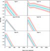 |
Fig. 2. Possible ranges of the K-band template light curves. The dark blue line is the median value and the light blue and red areas are the ranges within 1σ and 2σ, respectively. All parameters follow a Gaussian distribution, except for the H-poor templates. Their fastest possible evolution is limited to match the fastest SN in our template sample to avoid unrealistically rapid evolution. All templates are extrapolated with a linear tail phase. |
3.3.2. Host extinction
Unfortunately, the intrinsic distribution of host extinctions of CCSNe in LIRGs is uncertain. Using radio observations Mattila & Meikle (2001) estimated extinctions towards 19 SN remnants in the central 500 pc region of the nearby IR bright starburst galaxy M 82 finding a mean extinction of AV = 24 ± 9 mag. So far, the largest extinction towards a SN discovered at IR wavelengths is reported by Kankare et al. (2008) for SN 2008cs discovered at 1.5 kpc projected distance from the centre of the LIRG IRAS 17138−1017. However, the exact shape of the extinction distribution becomes irrelevant for our study at very high extinction, for example any SN suffering from a host extinction of AV ≳ 40 mag is equally unobservable in our dataset. Thus the shape of the high host extinction distribution is not important, but rather the fraction of the high extinction events. The host extinction of the simulated SNe in the Monte Carlo simulation was split into two components: A surface component, fraction taken into account with the extinction model, and an extremely obscured deep component that corresponds to the missing fraction. For the surface component, we fitted a set of host galaxy extinctions for 19 CCSNe discovered by previous optical or near-IR searches in central regions of LIRGs from Kankare et al. (2021) with an exponential function. The best fit resulted in a function P(AV) = 0.881e−0.084AV, with a median probability of AV = 7.7 mag (Fig. 3). The extinction values applied to the simulated CCSNe were randomly selected from this distribution. SNe in the missing fraction are considered to be completely undetectable, exploding at extremely dusty nuclear and circum-nuclear regions of their host galaxy. The probability was set before each run for a simulated SN to belong either to the surface extinction fraction or to the missing fraction, with the aim to constrain the latter. This missing fraction probability was varied between 0% and 99%. Galactic extinctions were based on the dust map calibration of Schlafly & Finkbeiner (2011) for the sample galaxies and were acquired from NASA/IPAC Extragalactic Database (NED), and are listed in Table 1. For comparison, the SED models used to derive the intrinsic CCSN rates in Sect. 3.3.4 assume the following extinction ranges for the different galaxy components: AV ≲ 20 mag for the diffuse dust component, AV ∼ 50 − 250 mag for the star-forming regions and giant molecular clouds, and AV ∼ 250 − 1500 mag for the AGN torus.
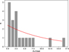 |
Fig. 3. Host extinction of CCSNe in central regions of LIRGs from Kankare et al. (2021) fitted with an exponential function (red curve) resulting in P(AV) = 0.881e−0.084AV. |
3.3.3. Control times
Total control time (TCT) is a measure of how long a galaxy has had an opportunity to produce detectable SNe within a survey (Zwicky 1938; Cappellaro et al. 1993), and is computed from individual control times (CT). For example, a five year survey with one year cadence would not automatically result in a TCT of five years, since many SNe could have potentially exploded and faded between the observations. Calculation of the CTs requires information on the absolute peak magnitude distribution and the light curve evolution for a given SN type, distance modulus, line-of-sight extinction, and the limiting magnitudes of the image. Therefore, the CT describes how long on average a SN could be detected. The descriptions of the adopted SN absolute peak magnitude distributions and light curve evolution are provided in the previous section.
For limiting magnitudes, each image epoch was handled separately. Each pixel in the limiting magnitude image was multiplied by a weight, equal to the ratio of the flux of the pixel compared to the total flux of the galaxy, and then their mean was calculated; this mean value was adopted as the limiting magnitude of the epoch for the purpose of the CT calculation. Subsequently, a Monte Carlo method was used to generate a total of 105 light curves of each SN subtype by applying absolute peak magnitude, timescale randomisation and random host extinction on the template light curves based on the parameters described in Table 2. For each light curve it was measured for how long the apparent magnitude of the SN was brighter than the flux weighted average limiting magnitude for that epoch. Finally, the CT for that epoch was estimated as the mean of those times. This process was repeated for each galaxy and each epoch in the dataset. Variance in repeated runs of this process was less than one day, which was the time resolution of the main Monte Carlo method.
To calculate the TCTs, the time differences between the observed epochs were summed, except if the time difference was larger than the CT, in which case the CT was used instead of the time difference. The CTs and TCTs were calculated for each CCSN subtype separately. The start date for the detection probability Monte Carlo simulation was the beginning date of the CT of the first observed epoch. In the process CCSNe were simulated only within the CT ranges. The median CT of the fastest evolving CCSN template IIb was 71 days.
3.3.4. Intrinsic CCSN rates
Intrinsic CCSN rates for the dataset were obtained with an adapted version of SED Analysis Through Markov Chains (SATMC) Monte Carlo code (Johnson et al. 2013; Efstathiou et al. 2022). The LIRG SEDs were constructed from a combination of archival photometry and spectra. Included were data from the Galaxy Evolution Explorer (GALEX), 2MASS, the Infrared Astronomical Satellite (IRAS), and the Infrared Space Observatory (ISO) photometric data via the NASA/IPAC Extragalactic Database and references therein. Photometric data was also obtained from the Data Release 2 of the Panoramic Survey Telescope and Rapid Response System (Pan-STARRS; Chambers et al. 2016), and the Herschel Space Observatory image atlas by Chu et al. (2017). Furthermore, Spitzer spectra used in a SED analysis by Herrero-Illana et al. (2017) were also employed.
The components of the radiative transfer model were as follows: starburst (Efstathiou et al. 2000; Efstathiou & Siebenmorgen 2009), AGN (Efstathiou & Rowan-Robinson 1995; Efstathiou et al. 2013), and a spheroidal galaxy (Efstathiou et al. 2021) or a disc galaxy (Efstathiou et al. 2022). SATMC method fits simultaneously the different model components to the SED of a galaxy to estimate the contribution of each component. The contribution of the starburst component constrains the total mass and age of the starburst. The model adopts the Salpeter initial mass function (IMF), solar metallicity and stellar population synthesis models of Bruzual & Charlot (2003). The model determines the starburst age from the SED fit and then follows the stellar population models to that age to determine the CCSN rate. The model assumes that the massive stars on their stellar tracks can explode as CCSNe up to an age of ∼42.6 Myr, corresponding to masses of ∼8 M⊙. However, since the starburst ages derived for the LIRGs in the dataset are younger than this, the exact lower mass limit of CCSNe is not critical. The intrinsic CCSN rate estimates were derived in this work for CGCG 049−057, IRAS 16516−0948, IRAS 17578−0400, and MCG+08-11-002 with the SED fits shown in Fig. 4. Intrinsic CCSN rates for IRAS 17138−1017, IC 883, and Arp 299-A/B were obtained from Kankare et al. (2021) and derived with the same method. Intrinsic CCSN rate for Arp 299-A/B was obtained for the combined system, which was divided between the A and B systems based on results by Mattila et al. (2012). The resulting CCSN rates, SFRs, and starburst ages from the SATMC are listed in Table 1.
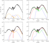 |
Fig. 4. Our SED models (solid black curves) for the observations (black points) of four sample LIRGs, including IRAS 17578−0400 (top left), MCG+08-11-002 (top right), CGCG 049−057 (bottom left), and IRAS 16516−0948 (bottom right). The model components include a spheroidal (dot dashed orange) or a disc (dot dashed green), starburst contribution (dashed red), and an AGN (dotted blue). We note that the starburst component of IRAS 17578−0400 dominates the total emission and is overlapped by the combined model curve, due to the small contribution of the other components. |
3.4. Error estimation
Due to the random nature of the Monte Carlo method, the impact of the individual sources of error become chaotic. The effect of this was estimated by running the main Monte Carlo program with selected parameters offset by their respective errors, for example the CCSN template peak luminosities increased by their 1σ variance, to evaluate its effect on the results. The relevant parameters and their respective errors are the following. First, the process of determining the limiting magnitudes for the images used a step of 0.2 mag, giving an error of ±0.2 mag. Next, for the photometric zero point calibration a conservative error of ±0.3 mag was estimated based on the largest difference between the photometric zero point corrections across the dataset. Another uncertainty to take into account is the error of the MR − MK colour difference to estimate the K-band peak magnitudes based on the R-band absolute peak magnitudes. H-poor templates had a standard deviation of ±0.26 mag and Type II templates a standard deviation of ±0.07 mag. Since the 87A-like and IIn templates had only one light curve on which the shift was based, they had no statistical error to use. Conservatively, we adopted the largest errors for this uncertainty. Finally, the error on the distance modulus for the galaxies from NED was ±0.15 mag. Thus, the overall error as the square root of the sum of squares is ±0.47 mag.
The number of intrinsic CCSNe predicted by the Monte Carlo simulation is small, and thus sensitive to small number statistics. Therefore, we adopt Poissonian confidence limits by Gehrels (1986) to the estimated number of events as their uncertainty.
Estimated percentage of recoverable CCSNe in the survey data of the sample galaxies, for different adopted missing fraction values.
Expected number of detected CCSNe for each galaxy in the dataset, for different missing fractions.
4. Results
The output of the Monte Carlo simulation is an average detection probability of SNe for each galaxy (i.e. the fraction of detectable CCSNe from the estimated intrinsic number of CCSNe, as a function of the missing fraction). These values are presented for all the sample galaxies in Table 3 for a selection of missing fraction values. The SATMC method has provided us with intrinsic CCSN rates for the galaxies in our sample. The intrinsic CCSN rates were split amongst all the CCSN subtypes according to rates by Shivvers et al. (2017), and then multiplied by their respective TCTs to acquire the intrinsic number of CCSNe of each subtype. An example for IC 883: The total CTs of different CCSN subtypes are 1.70, 1.82, 1.95, 2.16, 2.48, and 4.77 yr for the Type IIb, Ib, Ic, II, 87A-like, and IIn SNe, respectively. The intrinsic CCSN rate is 2.1 SN yr−1, which corresponds to 0.30, 0.34, 0.32, 2.79, 0.17, and 1.0 SN after adjusting the relative rates for the difference in CTs, and multiplying by the corresponding CTs. However, only a fraction of these are detected due to the combined effects of host extinction and light curve evolution bringing the SN brightness below the limiting magnitude at the explosion position. The resulting values are presented in Table 4 for a selection of missing fraction values. Figure 5 plots expected CCSN detections as a function of the missing fraction.
 |
Fig. 5. Number of expected CCSNe detections from the Monte Carlo simulation compared to the missing fraction. Red line: Total number of expected CCSN detections from the dataset over the survey period as a function of the missing fraction. Shaded red areas: 1σ and 2σ confidence areas for the total number of expected CCSN detections from the dataset over the survey period as a function of the missing fraction. Poissonian upper and lower limits due to small number statistics and the cumulative effect of other error sources are combined here. Dashed black: Number of real detected CCSNe in the survey. |
Based on the number of five detected CCSNe in the survey, we obtain a missing fraction of 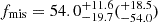 % with 1σ and (2σ) uncertainties. This is the missing fraction of CCSNe which have extremely high host extinctions and thus cannot be discovered by optical or NIR observations. Additionally, CCSNe not included in the missing fraction may also remain undiscovered due to moderate host extinctions. The fraction of these moderately obscured and undiscovered CCSNe depends on the survey depth and can be calculated by integrating the host extinction model curve over the relevant extinction range. Within the compiled sample of CCSNe discovered in the central regions of LIRGs by Kankare et al. (2021), the largest estimated host galaxy extinction among the reported optically discovered CCSNe was AV = 3.1 mag. Therefore, as an example, in the context of a survey that is able to detect objects up to AV = 3 mag, the fraction of CCSNe with AV ≤ 3 mag and AV > 3 mag is 22% and 78%, respectively, within the CCSNe not included in the missing fraction, resulting in the total fraction of undetectable CCSNe of
  %. Similarly for near-infrared surveys, choosing extinction threshold examples of AV = 13 and 16 mag, we obtain the total fractions of undetectable CCSNe of
  and
and  %, respectively. The limit AV = 16 was chosen as the highest host extinction of a SN in the dataset. The limit AV = 13 mag was calculated to be representative of the ALTAIR/NIRI dataset on average. The median limiting magnitude of the dataset was 19.4 mag, and the median luminosity distance was 74.7 Mpc. The extinction limit was then chosen as the amount of host extinction after which the most common CCSN subtype template, Type II, would remain detectable for its median CT of 100 days. The median galactic extinction AKGal for the dataset was 0.05 mag, and was thus assumed to be zero in this calculation.
In Table 5 we list the detected fraction of CCSNe with host extinctions within the P(AV) distribution below a detection threshold AV, limit calculated as fAV = ∫0AV, limitP(AV) dAV; the fraction of CCSNe that remain undetected due to host extinction described by the host extinction model calculated as fext = [(1 − fAV)×(1 − fmis)]; and the total undetected fraction calculated as the sum of the missing fraction and the fraction of CCSNe that remain undetected due to host extinction described by the host extinction model, ftot = fext + fmis. Surveys with deeper detection thresholds are able to detect more of the CCSN population not included in the missing fraction, which is assumed to remain always undetected.
Total undetectable fractions calculated from the missing fraction and the extinction model.
We additionally note that the median CT for the fastest evolving CCSN template (Type IIb) is 71 days. This suggests that a minimum cadence of ∼2 months is optimal for a similar survey as our dataset to expect to detect half of the Type IIb SNe that could be discovered in at least one epoch, assuming minimal extinction in K-band.
Comparing our undetectable fraction estimate of  % for infrared surveys with a limit of AV = 16 mag, we find very similar undetectable fraction to the one by Miluzio et al. (2013) of ∼60% to 75%. This is not surprising since we have very similar methods. Their galaxy sample is also similar including 30 starburst galaxies of which only one is a non-(U)LIRG and two are ULIRGs. They also performed their analysis in K-band, with a notable difference of using non-AO data for this.
Mattila et al. (2012) estimate that  % of CCSNe remain undetected by optical observations in LIRGs due to high host extinctions based on the reported discoveries of CCSNe in the nearby LIRG Arp 299. Assuming an optical survey extinction limit of 3 mag, our total fraction of undetectable CCSNe results in
  %, which is in good agreement with the results of Mattila et al. (2012). The intrinsic CCSN rate of Arp 299 in their work was calculated with SED fitting similarly to our work, but the A and B cores were treated separately, and the SED data was limited in wavelength coverage. The CCSN rate of the C nucleus (in combination with the C’ component) and the circumnuclear regions were determined from the empirical equation by Mattila & Meikle (2001) which estimates the CCSN rate based on the infrared luminosity of the LIRG. This resulted in a CCSN rate of 1.29 and 0.30 − 0.61 CCSN yr−1 for the nuclei and the circumnuclear regions, respectively. This work adopts the more recent results from Kankare et al. (2021) where the SED fit was carried out for the whole Arp 299 system with one SED that also includes a broader wavelength range, which resulted in a total CCSN rate of
  CCSN yr−1. The resulting CCSN rate was divided in this work between the A and B+C nuclei based on their IR luminosities.
Based on their results, Fox et al. (2021) missed ∼83% of the CCSNe in their sensitivity range. They estimated the intrinsic CCSN rates based on infrared luminosity with the equation by Mattila & Meikle (2001). Their undetected fraction of ∼83% is significantly higher than our 66% that we derive for AV = 16 mag host extinction limit, despite the similar wavelength of the search. They explain that the poor resolution of Spitzer and its asymmetric PSF result in strong image subtraction residuals and low sensitivity at the central regions of the sample galaxies. Therefore, a comparably higher undetected fraction can be expected.
The extinction calculations in this work have assumed the commonly used Cardelli et al. (1989) extinction law with RV = 3.1, which results in AK/AV = 0.114. For comparison, we calculated some of the survey thresholds with alternative reddening laws, including the Cardelli et al. (1989) extinction law with RV = 2.7 (Small Magellanic Cloud) and RV = 4.05 (starforming galaxy), the Calzetti et al. (2000) attenuation law with RV = 4.05, and the Fitzpatrick (1999) extinction law with RV = 3.1. These result in AK/AV ratios of 0.107, 0.124, 0.091, and 0.116, respectively. Converting these ratios for AV = 16 mag results in AK values of 1.8 mag for the Cardelli et al. (1989) law with RV = 3.1, and 1.7, 2.0, 1.5, 1.9 mag for the rest, respectively. Therefore, the differences are not large and are basically within one 0.2 mag step in our detection threshold simulations.
5. Conclusions
We have presented new estimates for the fraction of undetectable CCSNe in LIRGs in the local Universe with a detailed description of our method. The analysis is based on the SUNBIRD survey near-IR K-band monitoring dataset of eight LIRGs using the Gemini-North Telescope with the ALTAIR/NIRI laser guide star AO system, which has yielded detections of five CCSNe. We have also presented a new extinction distribution for CCSNe in the central regions of LIRGs P(AV) = 0.881e−0.084AV (with a median probability of AV = 7.7), based on the distribution of estimated extinctions for CCSNe discovered in the central regions of LIRGs at optical and near-IR wavelengths (Kankare et al. 2021). This distribution still excludes those CCSNe that have the highest extinctions and are accounted for in the missing SN fraction. Based on the analysed SUNBIRD dataset, the resulting missing fraction for CCSNe in LIRGs is  %.
%.
The total fraction of undetectable CCSNe depends on the survey detection threshold for the host galaxy extinction. The additional contribution to the undetectable fraction can be calculated by integrating over our adopted extinction model probability distribution above the extinction limit. For assumed typical examples of host extinction limits for near-infrared (AV = 16 mag) and optical (AV = 3 mag) surveys result in a total undetectable fraction of  % and
% and  %, respectively.
Transient surveys locally and at intermediate redshifts will be revolutionised by next-generation programmes like the Legacy Survey of Space and Time (LSST) of the Vera C. Rubin Observatory whereas the JWST will be able to probe the CCSN rates in the cosmic noon. Estimates for the undetected fraction of CCSNe in local LIRGs will be crucial for calibrating the CCSN rates derived by the LSST, JWST, and other next-generation facilities.
Acknowledgments
We thank the anonymous referee for useful comments. I.M. and E.K. acknowledge financial support from the Emil Aaltonen foundation. T.M.R. is part of the Cosmic Dawn Center (DAWN), which is funded by the Danish National Research Foundation under grant DNRF140. S.M. and T.M.R. acknowledge support from the Research Council of Finland project 350458. C.V. acknowledges financial support from the Vilho, Yrjö and Kalle Väisälä Fund. Based on observations obtained at the international Gemini Observatory, a program of NSF NOIRLab, which is managed by the Association of Universities for Research in Astronomy (AURA) under a cooperative agreement with the U.S. National Science Foundation on behalf of the Gemini Observatory partnership: the U.S. National Science Foundation (United States), National Research Council (Canada), Agencia Nacional de Investigación y Desarrollo (Chile), Ministerio de Ciencia, Tecnología e Innovación (Argentina), Ministério da Ciência, Tecnologia, Inovações e Comunicações (Brazil), and Korea Astronomy and Space Science Institute (Republic of Korea). Based on observations made with the Nordic Optical Telescope, owned in collaboration by the University of Turku and Aarhus University, and operated jointly by Aarhus University, the University of Turku and the University of Oslo, representing Denmark, Finland and Norway, the University of Iceland and Stockholm University at the Observatorio del Roque de los Muchachos, La Palma, Spain, of the Instituto de Astrofisica de Canarias. This publication makes use of data products from the Two Micron All Sky Survey, which is a joint project of the University of Massachusetts and the Infrared Processing and Analysis Center/California Institute of Technology, funded by the National Aeronautics and Space Administration and the National Science Foundation. This research has made use of the NASA/IPAC Extragalactic Database (NED), which is operated by the Jet Propulsion Laboratory, California Institute of Technology, under contract with the National Aeronautics and Space Administration.
References
- Alard, C. 2000, A&AS, 144, 363 [NASA ADS] [CrossRef] [EDP Sciences] [Google Scholar]
- Alard, C., & Lupton, R. H. 1998, ApJ, 503, 325 [Google Scholar]
- Anderson, J. P., González-Gaitán, S., Hamuy, M., et al. 2014, ApJ, 786, 67 [Google Scholar]
- Bertin, E., & Arnouts, S. 1996, A&AS, 117, 393 [NASA ADS] [CrossRef] [EDP Sciences] [Google Scholar]
- Bianco, F. B., Modjaz, M., Hicken, M., et al. 2014, ApJS, 213, 19 [Google Scholar]
- Borisov, G., Dimitrov, D., Semkov, E., et al. 2002, Inf. Bull. Var. Stars, 5264, 1 [Google Scholar]
- Botticella, M. T., Smartt, S. J., Kennicutt, R. C., et al. 2012, A&A, 537, A132 [NASA ADS] [CrossRef] [EDP Sciences] [Google Scholar]
- Botticella, M. T., Cappellaro, E., Greggio, L., et al. 2017, A&A, 598, A50 [NASA ADS] [CrossRef] [EDP Sciences] [Google Scholar]
- Bouchet, P., & Danziger, I. J. 1993, A&A, 273, 451 [NASA ADS] [Google Scholar]
- Bouchet, P., Moneti, A., Slezak, E., Le Bertre, T., & Manfroid, J. 1989, A&AS, 80, 379 [NASA ADS] [Google Scholar]
- Bruzual, G., & Charlot, S. 2003, MNRAS, 344, 1000 [NASA ADS] [CrossRef] [Google Scholar]
- Calzetti, D., Armus, L., Bohlin, R. C., et al. 2000, ApJ, 533, 682 [NASA ADS] [CrossRef] [Google Scholar]
- Cappellaro, E., Turatto, M., Benetti, S., et al. 1993, A&A, 268, 472 [Google Scholar]
- Cappellaro, E., Botticella, M. T., Pignata, G., et al. 2015, A&A, 584, A62 [NASA ADS] [CrossRef] [EDP Sciences] [Google Scholar]
- Cardelli, J. A., Clayton, G. C., & Mathis, J. S. 1989, ApJ, 345, 245 [Google Scholar]
- Chambers, K. C., Magnier, E. A., Metcalfe, N., et al. 2016, ArXiv e-prints [arXiv:1612.05560] [Google Scholar]
- Chu, J. K., Sanders, D. B., Larson, K. L., et al. 2017, ApJS, 229, 25 [Google Scholar]
- Dahlen, T., Strolger, L.-G., Riess, A. G., et al. 2012, ApJ, 757, 70 [NASA ADS] [CrossRef] [Google Scholar]
- DeCoursey, C., Egami, E., Pierel, J. D. R., et al. 2025, ApJ, 979, 250 [Google Scholar]
- Djupvik, A. A., & Andersen, J. 2010, Astrophys. Space Sci. Proc., 14, 211 [NASA ADS] [CrossRef] [Google Scholar]
- Efstathiou, A., & Rowan-Robinson, M. 1995, MNRAS, 273, 649 [Google Scholar]
- Efstathiou, A., & Siebenmorgen, R. 2009, A&A, 502, 541 [NASA ADS] [CrossRef] [EDP Sciences] [Google Scholar]
- Efstathiou, A., Rowan-Robinson, M., & Siebenmorgen, R. 2000, MNRAS, 313, 734 [Google Scholar]
- Efstathiou, A., Christopher, N., Verma, A., & Siebenmorgen, R. 2013, MNRAS, 436, 1873 [NASA ADS] [CrossRef] [Google Scholar]
- Efstathiou, A., Małek, K., Burgarella, D., et al. 2021, MNRAS, 503, L11 [Google Scholar]
- Efstathiou, A., Farrah, D., Afonso, J., et al. 2022, MNRAS, 512, 5183 [NASA ADS] [CrossRef] [Google Scholar]
- Ergon, M., Sollerman, J., Fraser, M., et al. 2014, A&A, 562, A17 [NASA ADS] [CrossRef] [EDP Sciences] [Google Scholar]
- Ergon, M., Jerkstrand, A., Sollerman, J., et al. 2015, A&A, 580, A142 [NASA ADS] [CrossRef] [EDP Sciences] [Google Scholar]
- Fassia, A., Meikle, W. P. S., Vacca, W. D., et al. 2000, MNRAS, 318, 1093 [Google Scholar]
- Filippenko, A. V. 1997, ARA&A, 35, 309 [NASA ADS] [CrossRef] [Google Scholar]
- Fitzpatrick, E. L. 1999, PASP, 111, 63 [Google Scholar]
- Fox, O. D., Khandrika, H., Rubin, D., et al. 2021, MNRAS, 506, 4199 [NASA ADS] [CrossRef] [Google Scholar]
- Gehrels, N. 1986, ApJ, 303, 336 [Google Scholar]
- Gruppioni, C., Béthermin, M., Loiacono, F., et al. 2020, A&A, 643, A8 [NASA ADS] [CrossRef] [EDP Sciences] [Google Scholar]
- Herrero-Illana, R., Pérez-Torres, M. Á., Randriamanakoto, Z., et al. 2017, MNRAS, 471, 1634 [Google Scholar]
- Hicken, M., Friedman, A. S., Blondin, S., et al. 2017, ApJS, 233, 6 [NASA ADS] [CrossRef] [Google Scholar]
- Hodapp, K. W., Jensen, J. B., Irwin, E. M., et al. 2003, PASP, 115, 1388 [Google Scholar]
- Horiuchi, S., Beacom, J. F., Kochanek, C. S., et al. 2011, ApJ, 738, 154 [NASA ADS] [CrossRef] [Google Scholar]
- James, P. A., & Anderson, J. P. 2006, A&A, 453, 57 [NASA ADS] [CrossRef] [EDP Sciences] [Google Scholar]
- Johnson, S. P., Wilson, G. W., Tang, Y., & Scott, K. S. 2013, MNRAS, 436, 2535 [Google Scholar]
- Kankare, E., Mattila, S., Ryder, S., et al. 2008, ApJ, 689, L97 [Google Scholar]
- Kankare, E., Mattila, S., Ryder, S., et al. 2012, ApJ, 744, L19 [Google Scholar]
- Kankare, E., Mattila, S., Ryder, S., et al. 2014, MNRAS, 440, 1052 [Google Scholar]
- Kankare, E., Efstathiou, A., Kotak, R., et al. 2021, A&A, 649, A134 [NASA ADS] [CrossRef] [EDP Sciences] [Google Scholar]
- Kennicutt, R. C. 1998, ARA&A, 36, 189 [NASA ADS] [CrossRef] [Google Scholar]
- Kool, E. C., Ryder, S., Kankare, E., et al. 2018, MNRAS, 473, 5641 [Google Scholar]
- Krisciunas, K., Hamuy, M., Suntzeff, N. B., et al. 2009, AJ, 137, 34 [Google Scholar]
- Le Floc’h, E., Papovich, C., Dole, H., et al. 2005, ApJ, 632, 169 [Google Scholar]
- Li, W. D., Filippenko, A. V., Treffers, R. R., et al. 2000, AIP Conf. Ser., 522, 103 [Google Scholar]
- Li, W., Leaman, J., Chornock, R., et al. 2011, MNRAS, 412, 1441 [NASA ADS] [CrossRef] [Google Scholar]
- Magnelli, B., Elbaz, D., Chary, R. R., et al. 2009, A&A, 496, 57 [NASA ADS] [CrossRef] [EDP Sciences] [Google Scholar]
- Magnelli, B., Elbaz, D., Chary, R. R., et al. 2011, A&A, 528, A35 [NASA ADS] [CrossRef] [EDP Sciences] [Google Scholar]
- Mannucci, F., Della Valle, M., & Panagia, N. 2007, MNRAS, 377, 1229 [NASA ADS] [CrossRef] [Google Scholar]
- Mattila, S., & Meikle, W. P. S. 2001, MNRAS, 324, 325 [Google Scholar]
- Mattila, S., Väisänen, P., Farrah, D., et al. 2007, ApJ, 659, L9 [Google Scholar]
- Mattila, S., Dahlen, T., Efstathiou, A., et al. 2012, ApJ, 756, 111 [Google Scholar]
- Melinder, J., Dahlen, T., Mencía Trinchant, L., et al. 2012, A&A, 545, A96 [NASA ADS] [CrossRef] [EDP Sciences] [Google Scholar]
- Miluzio, M., Cappellaro, E., Botticella, M. T., et al. 2013, A&A, 554, A127 [NASA ADS] [CrossRef] [EDP Sciences] [Google Scholar]
- Pérez-Torres, M., Mattila, S., Alonso-Herrero, A., Aalto, S., & Efstathiou, A. 2021, A&ARv, 29, 2 [CrossRef] [Google Scholar]
- Phillips, M. M. 1993, ApJ, 413, L105 [Google Scholar]
- Pozzo, M., Meikle, W. P. S., Fassia, A., et al. 2004, MNRAS, 352, 457 [CrossRef] [Google Scholar]
- Riello, M., & Patat, F. 2005, MNRAS, 362, 671 [Google Scholar]
- Schlafly, E. F., & Finkbeiner, D. P. 2011, ApJ, 737, 103 [Google Scholar]
- Shivvers, I., Groh, J. H., Mauerhan, J. C., et al. 2015, ApJ, 806, 213 [NASA ADS] [CrossRef] [Google Scholar]
- Shivvers, I., Modjaz, M., Zheng, W., et al. 2017, PASP, 129, 054201 [NASA ADS] [CrossRef] [Google Scholar]
- Skrutskie, M. F., Cutri, R. M., Stiening, R., et al. 2006, AJ, 131, 1163 [NASA ADS] [CrossRef] [Google Scholar]
- Smartt, S. J. 2009, ARA&A, 47, 63 [NASA ADS] [CrossRef] [Google Scholar]
- Soifer, B. T., Neugebauer, G., Matthews, K., et al. 2001, AJ, 122, 1213 [Google Scholar]
- Strolger, L.-G., Dahlen, T., Rodney, S. A., et al. 2015, ApJ, 813, 93 [NASA ADS] [CrossRef] [Google Scholar]
- Tody, D. 1986, SPIE Conf. Ser., 627, 733 [Google Scholar]
- Yuan, F., Jerkstrand, A., Valenti, S., et al. 2016, MNRAS, 461, 2003 [Google Scholar]
- Zwicky, F. 1938, ApJ, 88, 529 [Google Scholar]
Appendix A: Additional tables and figures
Survey epochs and CTs of Arp 299-A.
Survey epochs and CTs of Arp 299-B.
Survey epochs and CTs of CGCG 049-057 for each CCSN subtype.
Survey epochs and CTs of IC 883.
Survey epochs and CTs of IRAS 16516-0948.
Survey epochs and CTs of IRAS 17138-1017.
Survey epochs and CTs of IRAS 17578-0400.
Survey epochs and CTs of MCG+08-11-002.
All Tables
Estimated percentage of recoverable CCSNe in the survey data of the sample galaxies, for different adopted missing fraction values.
Expected number of detected CCSNe for each galaxy in the dataset, for different missing fractions.
Total undetectable fractions calculated from the missing fraction and the extinction model.
All Figures
|
Fig. 1. Galaxy IC 883 in different stages of determining the limiting magnitudes. (a) 22″ × 22″ median stacked image of the sample galaxy IC 883. (b) Galaxy map constructed from the median stacked image. (c) Example of a template subtraction. (d) Limiting magnitudes of IC 883 with the scale on the right. The two white pixels in the centre of the galaxy represent areas where persistent template subtraction artefacts prevented analysis; further details are provided in Sect. 3.2. (e) Example stamp positions for four sets of stamp lists. The red squares denote the non-varied stamps in the stamp lists and the blue squares denote the varied stamp. The positions of both sets was changed in a subsequent run to ensure that the whole galaxy was covered. (f) Example of the limiting magnitude iteration process. Visible point sources are simulated SNe at 16.8 mag, which are positioned on the galaxy map, excluding the stamp areas, separated by 7 × FWHM = 42 pixels. |
| In the text | |
|
Fig. 2. Possible ranges of the K-band template light curves. The dark blue line is the median value and the light blue and red areas are the ranges within 1σ and 2σ, respectively. All parameters follow a Gaussian distribution, except for the H-poor templates. Their fastest possible evolution is limited to match the fastest SN in our template sample to avoid unrealistically rapid evolution. All templates are extrapolated with a linear tail phase. |
| In the text | |
|
Fig. 3. Host extinction of CCSNe in central regions of LIRGs from Kankare et al. (2021) fitted with an exponential function (red curve) resulting in P(AV) = 0.881e−0.084AV. |
| In the text | |
|
Fig. 4. Our SED models (solid black curves) for the observations (black points) of four sample LIRGs, including IRAS 17578−0400 (top left), MCG+08-11-002 (top right), CGCG 049−057 (bottom left), and IRAS 16516−0948 (bottom right). The model components include a spheroidal (dot dashed orange) or a disc (dot dashed green), starburst contribution (dashed red), and an AGN (dotted blue). We note that the starburst component of IRAS 17578−0400 dominates the total emission and is overlapped by the combined model curve, due to the small contribution of the other components. |
| In the text | |
|
Fig. 5. Number of expected CCSNe detections from the Monte Carlo simulation compared to the missing fraction. Red line: Total number of expected CCSN detections from the dataset over the survey period as a function of the missing fraction. Shaded red areas: 1σ and 2σ confidence areas for the total number of expected CCSN detections from the dataset over the survey period as a function of the missing fraction. Poissonian upper and lower limits due to small number statistics and the cumulative effect of other error sources are combined here. Dashed black: Number of real detected CCSNe in the survey. |
| In the text | |
Current usage metrics show cumulative count of Article Views (full-text article views including HTML views, PDF and ePub downloads, according to the available data) and Abstracts Views on Vision4Press platform.
Data correspond to usage on the plateform after 2015. The current usage metrics is available 48-96 hours after online publication and is updated daily on week days.
Initial download of the metrics may take a while.