| Issue |
A&A
Volume 700, August 2025
|
|
|---|---|---|
| Article Number | A140 | |
| Number of page(s) | 12 | |
| Section | Planets, planetary systems, and small bodies | |
| DOI | https://doi.org/10.1051/0004-6361/202555209 | |
| Published online | 13 August 2025 | |
A circularly polarized low-frequency radio burst from the exoplanetary system HD 189733
1
LIRA, Observatoire de Paris, Université PSL, Sorbonne Université, Université Paris Cité, CY Cergy Paris Université, CNRS,
92190
Meudon,
France
2
Observatoire Radioastronomique de Nançay (ORN), Observatoire de Paris, Université PSL, Univ Orléans, CNRS,
18330
Nançay,
France
3
LUX, Observatoire de Paris, Université PSL, Sorbonne Université, CNRS,
75014
Paris,
France
4
Kapteyn Astronomical Institute, University of Groningen,
PO Box 800,
9700
AV
Groningen,
The Netherlands
5
Instituto de Astrofísica de Andalucía, Consejo Superior de Investigaciones Científicas (CSIC), Glorieta de la Astronomía s/n,
18008
Granada,
Spain
6
INAF,
via P. Gobetti 101,
40129
Bologna,
Italy
7
LPC2E, OSUC, Univ Orléans, CNRS, CNES, Observatoire de Paris,
45071
Orléans,
France
8
Department of Astronomy and Carl Sagan Institute, Cornell University,
Ithaca,
NY,
USA
9
Aix Marseille Université, CNRS, CNES, LAM,
Marseille,
France
10
Université Paris Cité and Université Paris Saclay, CEA, CNRS, AIM,
91190
Gif-sur-Yvette,
France
11
Institute of Radio Astronomy,
Mystetstv St. 4,
61002
Kharkiv,
Ukraine
★ Corresponding author: This email address is being protected from spambots. You need JavaScript enabled to view it.
Received:
18
April
2025
Accepted:
18
June
2025
Abstract
Aims. We aim to detect low-frequency radio emission from exoplanetary systems to gain insights into planetary magnetic fields, star–planet interactions, stellar activity, and exo-space weather. The HD 189733 system, hosting a well-studied hot Jupiter, is a prime target for such searches.
Methods. We conducted NenuFAR imaging observations in the 15–62 MHz range to cover the entire orbital phase of HD 189733 b. Dynamic spectra were generated for the target and other sources in the field, followed by a transient search in the time-frequency plane. The data processing pipeline incorporated direction-dependent calibration and noise characterization to improve sensitivity. We also searched for periodic signals using a Lomb–Scargle analysis.
Results. A highly circularly polarized radio burst was detected at 50 MHz, with a flux density of 1.5 Jy and a significance of 6σ at the position of HD 189733. No counterpart was found in Stokes I, likely because the emission is embedded in confusion noise and remains below the detection threshold. The estimated minimum fractional circular polarization of 38% suggests a coherent emission process. A periodicity search revealed no weaker signals linked to the planet’s orbital period, the star’s rotational period, or the synodic period and harmonic period between them. The burst’s properties are consistent with cyclotron maser instability (CMI) emission, however, the origin remains ambiguous. A comparison with theoretical models suggests star–planet interaction or stellar activity as potential origins. Alternative explanations such as contamination from other sources along the line of sight (e.g. the companion M dwarf) or noise fluctuation are plausible.
Key words: techniques: interferometric / planets and satellites: magnetic fields / planet-star interactions
NHFP Sagan Fellow, USA
© The Authors 2025
 Open Access article, published by EDP Sciences, under the terms of the Creative Commons Attribution License (https://creativecommons.org/licenses/by/4.0), which permits unrestricted use, distribution, and reproduction in any medium, provided the original work is properly cited.
This article is published in open access under the Subscribe to Open model. This email address is being protected from spambots. You need JavaScript enabled to view it. to support open access publication.
1 Introduction
The study of magnetic fields in exoplanetary systems is a vital frontier in astrophysics, offering profound insights into multiple planetary characteristics and phenomena (Zarka et al. 2015a; Lazio et al. 2016, 2019). Magnetic fields provide key windows into the interior structures and dynamos of exoplanets, in way that is analogous to to Jupiter and other Solar System planets (Hess & Zarka 2011; Bonati et al. 2021). Furthermore, understanding the magnetospheres of exoplanets is essential for grasping the complex dynamics of star–planet interactions (SPI), which can significantly influence planetary environments (Ip et al. 2004; Zarka 2007; Lanza 2009; Scharf 2010; Strugarek et al. 2015; Callingham et al. 2024; Zarka 2025). The presence and nature of magnetic fields are also pivotal in assessing the habitability of exoplanets, as they can shield atmospheres from stellar wind and cosmic radiation, while possibly mitigating atmospheric escape (Horner & Jones 2010; See et al. 2014; Gronoff et al. 2020; Carolan et al. 2021). Lastly, the detection and study of exoplanetary magnetic fields represent a potential avenue for the discovery and characterization of exoplanets, offering valuable methods for inferring the presence of planets beyond traditional transit and radial velocity techniques (Lazio 2018).
Magnetic fields within exoplanetary systems can be probed through various observational methods. Among these, radio observations stand out as particularly advantageous as this method enables the direct constraint of magnetic field amplitudes without relying on complex modeling assumptions and exhibits a reduced susceptibility to false positives (Grießmeier 2015; Zarka 2025). The predominant mechanisms for planetary radio emissions are cyclotron maser instability (CMI) (Zarka 1998; Treumann 2006) and synchrotron radiation (de Pater 2004), with a current research emphasis on CMI due to its high efficiency.
Overall, CMI emissions are highly circularly polarized, strongly beamed, and temporally variable (Zarka et al. 2004). They are produced near the local electron cyclotron frequency (fce), which directly links the observed emission to the amplitude of the local magnetic field strength at the source of the emission (Zarka et al. 2015a). The emission spectrum shows a sharp cutoff at a maximum frequency set by the strongest magnetic field, typically near the planetary surface. For CMI to operate, the local plasma frequency, fpe, must satisfy fpe/ fce < 0.1 (Treumann 2006); otherwise, the emission is suppressed. Furthermore, CMI is strongly anisotropic and beamed along a narrow hollow cone at large angles (70°–90°) from the local magnetic field direction (Pritchett 1986; Hess et al. 2008; Louis et al. 2017). This beaming geometry implies that detection depends on the observer’s viewing angle.
The quest to detect radio emissions from exoplanets has spanned several decades, predominantly yielding non-detections (Bastian et al. 2000; Farrell et al. 2004; Hallinan et al. 2013; Murphy et al. 2015; Lynch et al. 2017, 2018; O’Gorman et al. 2018; de Gasperin et al. 2020a). Despite these challenges, there have been multiple reports of tentative detections, such as 150 MHz radio emissions possibly emanating from exoplanets observed with the Giant Metrewave Radio Telescope (GMRT) (Lecavelier des Etangs et al. 2013; Sirothia et al. 2014), alongside GHz-band radio pulses that may have planetary origins (Bastian et al. 2018). Recent findings include the potential identification of auroral emissions, reminiscent of star–planet interactions, utilizing the Low-Frequency Array (LOFAR) and the Australia Telescope Compact Array (ATCA) (Vedantham et al. 2020; Callingham et al. 2021; Pérez-Torres et al. 2021; Turner et al. 2021). In particular, Tasse et al. (2025) have developped a new approach to generate massive amount of dynamic spectra from interformetric data. For the first time, Tasse et al. (2025) detected two bursts originated from stars hosting exoplanets, potentially revealing the first radio signatures of star–planet interactions via CMI. These intriguing observations underscore the need for meticulous follow-up studies to ascertain the planetary nature of the detected signals.
HD 189733, a binary star system located 19 parsecs from Earth, has emerged as a compelling target for radio astronomical studies, particularly due to its strong magnetic field and prior tentative detections. The system comprises a K-type primary star (HD 189733 A) and an M dwarf companion (HD 189733 B), separated by approximately 216 AU (Bakos et al. 2006). Orbiting the primary is a hot Jupiter, HD 189733 b, characterized by a short orbital period of 2.219 days and a semi-major axis of 0.0313 ± 0.0004 AU, with mass and radius estimates of 1.15 ± 0.04 MJ and 1.26 ± 0.03 RJ1, respectively (Bouchy et al. 2005). The orbital inclination of the planet with respect to the observer’s line of sight is approximately 85.7° (Boisse et al. 2009), indicating an almost edge-on orbit. Spectroscopic measurements have shown that the planet’s orbital plane is closely aligned with the stellar equator, with a projected spin–orbit angle of only 1.4° (Brogi et al. 2016). This implies that the planet transits near the stellar equator, and that our line of sight is nearly in the equatorial plane of the star.
Observational efforts have focused on delineating the magnetic properties of both the star and the orbiting exoplanet. Zeeman-Doppler imaging has mapped the stellar surface magnetic field, revealing strengths up to 40 G, and further monitoring has indicated variations in the planetary magnetic field correlating with stellar activity (Fares et al. 2010, 2017). Archival analyses of Ca II K spectral lines have detected modulations consistent with the exoplanet’s orbital period, suggesting star–planet interactions (SPI) (Cauley et al. 2018). This hypothesis is supported by X-ray observations from XMM-NEWTON and Chandra, highlighting the primary star’s high activity level and discrepancies in magnetic activity that may result from tidal interactions between the primary star and the exoplanet HD 189733 b (Pillitteri et al. 2010; Poppenhaeger et al. 2013; Pillitteri et al. 2014; Bourrier et al. 2020; Pillitteri et al. 2022).
In the radio domain, a 2.7 σ detection at 150 MHz by GMRT has been reported, although the sensitivity was insufficient to measure time variations that would allow us to firmly associate the emission with the planet (Lecavelier Des Etangs et al. 2011). Stellar wind modeling, informed by the measured magnetic field maps, suggests that planetary emissions should occur at 2–25 MHz; however, emission below 21 MHz might be obstructed by the stellar wind (Kavanagh et al. 2019). Additional stellar wind modeling suggests that a stretch-and-break SPI mechanism (Lanza 2013) could explain the observed signals (Strugarek et al. 2022), although further work on the applicability of the model (Callingham et al. 2024) and observations covering the entire orbital phase of the exoplanet are needed to confirm these findings. However, subsequent multi-wavelength analysis and observations, including some with Arecibo, caution that these tentative detections might be false positives. In such cases, the observed magnetic enhancements would be attributed to stellar activity, rather than to SPI (Route 2019; Route & Looney 2019).
To delve deeper into the potential SPI scenario, we conducted NenuFAR observations covering the full orbital phase of HD 189733 b across a broad low-frequency range. This approach is well suited to detecting beamed, low-frequency CMI emission induced by SPI, while also covering potential stellar plasma emission. Section 2 outlines the observational parameters and our comprehensive approach to covering the entire orbital phase of the system. Section 3 details the data processing pipeline used to calibrate, image, and analyze the dataset. Our results are presented in Section 4, including the detection of a highly circularly polarized burst and a search for periodic signals. In Section 5, we discuss possible origins of the detected burst, considering star–planet interaction, intrinsic stellar activity, and contamination from background sources. Finally, Section 6 summarizes our findings and outlines recommendations for future observations.
2 Observations
Our study utilizes the NenuFAR array in Nançay (New extension in Nançay upgrading LOFAR; see Zarka et al. 2012, 2015b, 2020). Designed as a low-frequency phased array and interferometer, NenuFAR operates within the 10–85 MHz range. The array is organized into hexagonal clusters of 19 dual-polarization antennas, each cluster called a mini-array (MA). The MAs are analog-phased, which results in a steerable instantaneous field of view (FoV) of 8° (85 MHz) to 60° (10 MHz). As of mid-2023 (the epoch of our observations), the array configuration includes 80 MAs positioned within a core area spanning 400 meters, complemented by 4 remote MAs situated at distances reaching up to 3 km.
Between June and October 2023, we conducted an observational campaign targeting the HD 189733 system using NenuFAR. These observations were conducted in a dual-mode setup, enabling simultaneous imaging and beamformed data collection. However, this paper focuses solely on the analysis of imaging data2. The specific parameters for the imaging observations are detailed in Table 1. To minimize the effect of ionospheric disturbance at the lower end of the frequency spectrum, observations were conducted at night, when the target’s elevation exceeded 40 degrees. Each night’s observation spanned several hours, adopting a tracking mode to maintain the target at the pointing center. For each observation, a 15-minute slot was allocated to observing a calibrator, either Cyg A or Cas A, either immediately before or after the primary observation period.
To comprehensively investigate the emissions from HD 189733 b, our observational campaign was carefully planned to span the exoplanet’s full orbital phase. This strategy stems from the anticipation that CMI emissions are beamed, becoming detectable from Earth only during specific segments of the orbital cycle (Lamy et al. 2023). The exoplanet’s orbital parameters were derived from transit timing observations by the TESS mission (Ivshina & Winn 2022). Figure 1 illustrates the orbital coverage achieved by our campaign. Over a cumulative observation duration of 103 hours, our observations covered most of HD 189733 b’s orbital phase, despite minor gaps introduced by the removal of low-quality data (see Section 3.2).
Observational parameters for the NenuFAR campaign targeting HD 189733.
3 Data reduction
Our data processing pipeline3 integrates a suite of software tools designed for NenuFAR and LOFAR datasets, leveraging the capabilities of Nenupy (Loh & the NenuFAR team 2020), Nenucal4 (Munshi et al. 2024), DP3 (van Diepen et al. 2018), AOFlagger (Offringa et al. 2012), DDFacet (Tasse et al. 2018), KillMS (Tasse 2014; Smirnov & Tasse 2015; Tasse 2023), DynspecMS (Tasse et al. 2025), and WSClean (Offringa et al. 2014). Prior to processing with our pipeline, initial preprocessing steps were performed following standard NenuFAR routines, including averaging and initial flagging of radio frequency interference (RFI). Subsequently, our pipeline executes the following comprehensive sequence: (1) identification and removal of “bad” MAs at time of observation (due to temporary issues such as electronic failure or maintenance) and of RFI; (2) initial calibration using observations of known calibrators; (3) direction-dependent (DD) calibration for mitigating pollution by prominent A-team sources (Cyg A, Cas A, Tau A and Vir A de Gasperin et al. 2020b); (4) dynamic spectra generation across various directions within the FoV; (5) application of source-finding algorithms in the dynamic spectra to identify relevant signals. A step-by-step depiction of these pipeline stages is presented in Figure 2.
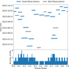 |
Fig. 1 Orbital phase coverage of HD 189733 b observations. HD 189733 b is a transiting exoplanet, with the orbital phase of 0 defined as the moment of its transit (Ivshina & Winn 2022). Observations marked in gray represent the data excluded from scientific analysis due to poor quality. |
3.1 The pipeline
First, flagging operations were applied to both the calibrator and the target data to ensure their quality. Utilizing a predefined list of channels known to be contaminated by RFI from previous observations, we proactively flagged these channels. Additionally, AOFlagger was employed for automatic RFI detection and flagging. The identification of malfunctioning MAs involves an iterative approach: an extra calibration round using the calibrator data precedes the examination of the calibration solutions, considering both amplitude and phase. Should the calibration solutions reveal significant discontinuities for any MA, the MA would then be designated as faulty, leading to the flagging of all associated baselines. On average, approximately 7% of MAs were flagged during the observations.
Following the flagging process, we proceeded with the initial full-Stokes calibration, which is direction-independent and utilizes observations of calibrators. This calibration was done with DP3, leveraging models of A-team sources comprising of point sources and Gaussians. The amplitude and phase calibration solutions derived from this step were then transferred to and applied on the target observations.
Then, we applied full-Stokes direction-dependent calibration to mitigate the influence of contaminating A-team sources on the visibilities. Given their prominence in the low-frequency radio sky, A-team sources can degrade data quality even when located within the sidelobes outside the FoV. Direction-dependent calibration is beneficial at low frequencies due to the pronounced spatial variation in calibration solutions, which arises from ionospheric disturbances and the receiver beam’s shape (Smirnov 2011). The direction-dependent calibration process unfolds in stages: initially, DDFacet is utilized to produce a deconvoluted (“cleaned”) image of the FoV, from which a sky model of sources within the FoV can be derived. Subsequently, models of the A-team sources are incorporated into this sky model. A calibration tailored to multiple directions is then conducted using KillMS, enabling the subtraction of A-team source contributions from the visibilities and isolating sources of moderate flux for further analysis.
To facilitate the search for transients within our dataset, we first generated the residual visibilities by removing the detected radio continuum sources. This involves conducting multifrequency-synthesis (MFS) imaging across the entire bandwidth to create a comprehensive sky model of the continuum sources within our FoV via clean deconvolution. Next, we subtracted these continuum sources from the visibilities, thus obtaining the residual visibilities primed for the analysis and detection of transients in the time-frequency plane.
We generated Stokes IQUV dynamic spectra from residual visibilities with DynspecMS, for the target direction (referred to as the “ON” beam) and for approximately 400 off-target directions (referred to as “OFF” beams) within NenuFAR’s FoV. The “OFF” beams, which are used to estimate the noise level5, were systematically spaced one degree apart using the Fibonacci lattice method for even distribution (Swinbank & James Purser 2006). Although dynamic spectra were created for all the Stokes parameters, our analysis specifically focused on the Stokes I and V components. This selection is based on the fact that CMI emissions are highly circularly polarized, making the Stokes V spectra particularly relevant for our study. Additionally, the noise level in Stokes V spectra is significantly lower compared to Stokes I, further improving the detection sensitivity. Nevertheless, Stokes Q and U were also examined for verification purposes in the event of potential detections. A graphical representation mapping all beam directions is presented in Figure 3.
The target dynamic spectra derived directly from the visibilities require a ‘flattening’ process to standardize the noise levels, which fluctuate across time and frequency. To achieve this, we first computed the mean and standard deviation (STD)6 for each time and frequency cell across approximately 400 “OFF” beams in the dynamic spectra, leveraging the consistency of apparent flux noise levels in various directions. Dynamic spectra corresponding to the scientific target were excluded from these calculations to avoid including genuine signals in our noise estimation. Finally, we normalized the noise levels by subtracting the mean noise level at each time-frequency pixel (averaged across all OFF beams) and dividing by the corresponding standard deviation.
Given the uncertain time/frequency widths of potential bursts, we applied a convolution process to the normalized dynamic spectra using Gaussian kernels across a range of resolutions. Time resolutions were set on a logarithmic scale, ranging from 16 seconds to 4096 seconds with a factor of 2, while frequency resolutions also followed a similar logarithmic progression, from 240 kHz to 15.36 MHz. For each combination of time and frequency resolution, we recalculated the mean and STD dynamic spectra across the “OFF” beams. Subsequently, we computed the signal-to-noise ratio (S/N) dynamic spectra by subtracting the mean from the convolved dynamic spectra and dividing with the corresponding STD.
Our search for individual transient candidates within the S/N dynamic spectra focused on identifying events with an S/N exceeding 5. This threshold ensures that the detected event is localized to the target direction, helping to distinguish genuine transients from RFI bursts, which would affect a broader area of the sky.
Upon identifying a transient candidate, we conducted a verification process by re-imaging the specific time and frequency range of the candidate using WSClean7, generating an all-sky image that includes a sidelobe area. This step helps rule out RFI contamination, ionospheric scintillation, sidelobe contamination, or noise peaks. Our approach follows a method similar to that described by Tasse et al. (2025), who highlight the potential biases introduced by time-frequency weighting and demonstrate a framework to assess detection reliability using re-weighted PSF testing. To ensure thoroughness, we employed a clustering algorithm that expands to include neighboring time/frequency cells exhibiting S/N values greater than 3, adjacent to the initial bursting range. A bright RFI is typically identified and verified within the dynamic spectra, appearing as either narrow-band signals at specific frequencies or as broadband signals with very short timescales and high brightness. Fainter RFI signals can be identified through re-imaging, as RFI typically affects multiple positions or even the entire FoV. Ionospheric scintillations are identified by re-imaging and checking for evidence of strong scintillation across the sky region, as they generally affect multiple sources rather than a single source. Sidelobe contamination can be identified by checking whether known bright sources appear at positions corresponding to sidelobes. Noise peaks are identified by re-imaging the suspected event; if no source resembling the PSF shape is visible in the image at the location of our target, the event is classified as an artifact. In cases where the imaged source matches the PSF, the event is confirmed as a transient candidate.
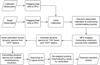 |
Fig. 2 Flowchart illustrating the stages of the data processing pipeline employed in the HD 189733 observational campaign with NenuFAR. |
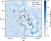 |
Fig. 3 Spatial distribution of dynamic spectra directions within the FoV, illustrated against a blue background created from a full-band MFS image prior to continuum source subtraction. The central red dot denotes the “ON” beam located in the direction of HD 189733. Orange dots represent the “OFF” beams, whose dynamic spectra are used for noise estimation. The black circle at the top marks the location of Cygnus A, which has been subtracted from visibilities. |
3.2 Data quality
Before performing scientific analysis, we assessed the quality of the data. Out of the 103 hours of observations collected during our campaign, 16 hours were deemed to be of poor quality, primarily due to thunderstorms and temporary instrumental failures. As a result, only 87 hours of data were retained for further analysis. Additionally, RFI flagging revealed that channels below 21 MHz were heavily contaminated by RFI, leading to their exclusion from further processing.
Given our focus on detecting potential CMI emissions, which are expected to exhibit strong circular polarization, it was essential to evaluate the level of polarization leakage in our data. Leakage occurs when signals from one polarization state contaminate another, potentially causing unpolarized sources to appear polarized or distorting the measured polarization fraction of polarized sources. In circular polarization, leakage typically arises in two ways: from total intensity into circular polarization or between linear and circular polarization (Sault et al. 1996; Lenc et al. 2017, often referred to as the “XY phase” issue). To quantify the leakage from total intensity into Stokes V, we compared pixel values of bright 3C sources in Stokes V and Stokes I images, estimating a leakage factor of approximately 0.75%. For leakage between linear and circular polarization, we measured the XY phase using observational data collected during a Jupiter burst, which is a strong polarized source below 40 MHz. At an S/N of about 1800, no significant leakage between linear and circular polarization was detected.
Following the leakage estimation, we assessed the noise level in our Stokes V data using both images and dynamic spectra, and compared these results with the expected thermal noise. At high time-frequency resolutions (e.g., 8 s × 195 kHz), the noise in the Stokes V data is primarily dominated by thermal noise. The lowest noise level (1.42 Jy/beam), about twice the theoretical thermal noise (0.67 Jy/beam), was observed around 50 MHz. At 21 MHz, the noise increased to nearly six times the thermal noise, likely due to ionospheric disturbances that are more pronounced at lower frequencies. However, we also note that leakage from Stokes I into Stokes V introduces additional confusion noise. For long integrations over wide frequency bands (e.g., 1 hour × 10 MHz), the noise level closely matches the estimated leaked confusion noise, making it challenging to detect signals below 50 mJy in our observations. Figure 4 illustrates the estimated noise levels for our observations. The leaked confusion noise was calculated by multiplying the leakage factor by the theoretical confusion noise in total intensity.
Besides the analysis presented in this work, the reliability of our data processing pipeline and transient search methodology is further supported by detections made in other projects using NenuFAR. Using the same pipeline, we successfully identified broadband, polarized emissions from Starlink satellites, demonstrating their impact on low-frequency radio astronomy (Bassa et al. 2024; Zhang et al. 2025). Additionally, we detected low-frequency radio bursts from other stellar and substellar systems, including repeating bursts likely originating from brown dwarfs (Zhang et al., in prep.), reinforcing the robustness of our approach when applied to astrophysical targets.
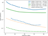 |
Fig. 4 Noise levels in the Stokes V data as achieved by the pipeline. The blue lines represent the measured noise levels from the observational data for two time-frequency integrations (8 s × 195 kHz and 1 hour × 10 MHz), derived from both dynamic spectra and images. The green lines indicate the theoretical thermal noise of NenuFAR for the same time-frequency integrations. The orange line represents the estimated confusion noise in Stokes V, caused by the 0.75% leakage from Stokes I. |
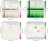 |
Fig. 5 Dynamic spectra of the HD 189733 field, showing the detection of a burst after convolution. Top-left panel: original Stokes V dynamic spectrum of HD 189733, at a resolution of 8 s × 195 kHz. The frequency range 41–43 MHz and the time range of 2–5 min are affected by RFI or temporary instrumental issues. The solid grey box marks the time-frequency region of the detected burst, though it is not visible at the native resolution. A dashed grey box, located at the same frequencies but earlier in time, serves as a control region for comparison. Top-right panel: noise dynamic spectrum, showing the standard deviation computed from ~400 off-beam directions for each time-frequency pixel. RFI-contaminated regions appear with elevated noise. Bottom-left panel: normalized Stokes V dynamic spectrum after applying noise standardization. This process flattens the noise level across the spectrum and down-weights contaminated regions. Bottom-right panel: convolved Stokes V dynamic spectrum with a resolution of 40 s × 4 MHz. The burst becomes clearly visible in the solid grey box, while no signal is seen in the control region (dashed grey box). Edge frequencies are excluded due to insufficient convolutional data. |
4 Results
Over the course of 87 hours of observations, only one transient candidate successfully passed the verification process described earlier8. This event is a 1.5 Jy circularly polarized burst, detected in the Stokes V dynamic spectrum of HD 189733 and confirmed through imaging. In addition to the search for individual bursts, we conducted a statistical analysis of possibly weaker emission from the system using the Lomb–Scargle method, aimed at identifying potential periodic signals. However, no significant periodicity was detected.
4.1 Individual burst
The burst was detected in the Stokes V dynamic spectra on 2023-09-28 at 21:18 UTC, when the exoplanet was at an orbital phase of 0.0197 (close to transit). At the original dynamic spectrum resolution of 8 s × 195 kHz, the burst was not detectable. However, after convolving the dynamic spectra to a lower time-frequency resolution of 40 s × 4 MHz, the burst exceeded the 5 σ threshold (Figure 5). The emission was detectable for approximately 96 seconds and spanned the frequency range 47.6–52.1 MHz. The actual time-frequency extent may be larger, as only the peak of the burst may have been detected due to sensitivity limits.
Re-imaging the data over the time and frequency range of the emission revealed a 6σ circularly polarized burst with a flux density of 1.5 Jy at the location of HD 189733 (Figure 6), confirming the detection. No corresponding burst was detected in the corresponding Stokes I image, indicating that the burst is highly circularly polarized. The noise level in the Stokes I image is approximately 1.3 Jy/beam, versus 0.25 Jy/beam in Stokes V9. Assuming that no detection means the Stokes I emission from HD 189733 is below the 3 σ threshold, the 1.5 Jy burst in Stokes V corresponds to a minimum fractional circular polarization of 38%. Additionally, leaked signals from bright Stokes I sources (such as 3C 409) were observed. Assuming that the bright background sources are unpolarized, we estimate the leakage level to be approximately 0.73%, ruling out instrumental leakage as the origin of the burst.
To investigate possible multi-wavelength counterparts, we searched the TESS archive10 for optical observations, but found no available data at the time of detection. A search in the HEASARC archive11 similarly yielded no overlapping UV/X-ray observations. We also checked the CHEOPS Science Archive12, which provides high-precision photometry of exoplanet host stars, but found no observations of HD 189733 around the burst time. Additionally, no relevant light curves were available from the NASA Exoplanet Watch13, a citizen science project that collects optical transit data from a global network of amateur and professional astronomers.
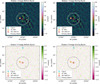 |
Fig. 6 Imaging verification of a 6σ burst in the direction of HD 189733 with NenuFAR. All the panels show apparent flux images to ensure consistent noise levels beyond the primary beam. Top-left panel: Stokes I image of the FoV before the burst, generated from visibilities corresponding to the control time-frequency range (dashed grey boxes) in dynamic spectra. The orange circle marks the 200 Jy radio source 3C 409, while the red circle marks the location of HD 189733. The cyan circle marks the location of Cyg A, which was subtracted from the visibilities. The large dashed grey circle represents the primary beam area of NenuFAR at 50 MHz (the central frequency of the detection). Top-right panel: Stokes I image corresponding to the burst’s time-frequency range (as indicated by the solid grey boxes in the dynamic spectra). Due to the relatively high noise level in Stokes I, no significant emission is detected at the location of HD 189733, while the bright source 3C 409 is clearly visible. Bottom-left panel: Stokes V image of the FoV generated from the control time-frequency range. The orange circle indicates the leakage at the location of 3C 409, while no significant emission is detected at the position of HD 189733 (red circle). Bottom-right panel: Stokes V image corresponding to bursting time-frequency range. The leakage at the location of 3C 409 is still visible (orange circle) and the red circle highlights a burst detected at the location of HD 189733. |
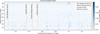 |
Fig. 7 Lomb–Scargle power distribution as a function of period (represented by the Lomb–Scargle frequency on the x-axis) and radio frequency (y-axis), based on the Stokes V dynamic spectra at the highest time-frequency resolution (8 s × 195 kHz). Orange dashed lines mark periods of scientific interest: the stellar rotation period, the orbital period of the planet, and the synodic period and the harmonic period between the two. The peaks near 1 cycle/day are likely caused by observational windowing. Only peaks with a low false alarm probability (FAP < 0.01) are considered significant. |
4.2 Search for periodicity
The detectability of cyclotron maser emissions depends strongly on the viewing geometry, as the emission is highly beamed along a thin hollow cone (Marques et al. 2017; Lamy et al. 2023). Detecting periodicity in the dynamic spectra could provide insights into the burst’s origin, particularly if the detected periods match known system timescales, such as the orbital period of the planet or the synodic period between it and the rotation of the stellar magnetic field (Louis et al. 2025). To investigate this possibility, we applied the Lomb–Scargle periodogram technique (VanderPlas 2018) to all convolved dynamic spectra across multiple time-frequency resolutions. False alarm probabilities (FAPs) were estimated using the Baluev method (Baluev 2008), which utilizes extreme value theory to provide an analytic upper limit for the FAP, reducing the need for extensive Monte Carlo simulations. We searched for periodic signals over the range of 0.74–35.82 days, covering key system timescales:
The minimum period (0.74 days) corresponds to one-third of the planet’s orbital period.
The maximum period (35.82 days) is three times the stellar equatorial rotation period.
This range includes important system periods:
Planetary orbital period: 2.22 days;
Stellar equatorial rotation period: 11.94 days;
Synodic period between the planet and star: 2.73 days,
![Mathematical equation: $\[P_{\text {synodic }}=\frac{1}{\left|\frac{1}{P_{\text {planet }}}-\frac{1}{P_{\text {star }}}\right|};\]$](/articles/aa/full_html/2025/08/aa55209-25/aa55209-25-eq1.png)
Harmonic period between the planet and star: 1.87 days,
![Mathematical equation: $\[P_{\mathrm{harmo}}=\frac{1}{\left(\frac{1}{P_{\mathrm{planet}}}+\frac{1}{P_{\mathrm{star}}}\right)}.\]$](/articles/aa/full_html/2025/08/aa55209-25/aa55209-25-eq2.png)
Additionally, since the host star undergoes differential rotation, this range includes its polar rotation period (16.53 days) (Fares et al. 2010) as well.
No periodic signals corresponding to the planetary orbit, stellar rotation, or anticipated star–planet interaction timescales were detected. The only significant periodicity appeared at 60 MHz with a period of 24 hours, probably caused by RFI and/or observational windowing, rather than an astrophysical source. The Lomb–Scargle power distribution and corresponding FAP analysis are shown in Figure 7.
5 Discussion
Identifying the origin of a single 6σ burst without an accompanying periodic signal is a challenge. To assess possible explanations, we examined the burst in the context of different emission mechanisms and compare theoretical predictions with the observed properties. We first explored whether the burst could be attributed to star–planet interaction, followed by an analysis of intrinsic stellar radio activity. We then investigated the possibility that the burst originated from a background source along the line of sight, before considering the potential for a false positive due to noise fluctuations.
5.1 Star–planet interaction
Star–planet interactions (SPI) can produce radio bursts through two primary mechanisms (Callingham et al. 2024; Zarka 2025). The first, sub-Alfvénic interaction, is analogous to the Jupiter-Io system. In this scenario, a planet, either intrinsically magnetized or conductive with an induced magnetosphere, orbits within the Alfvén surface of its host star, standing an obstacle to the stellar plasma flow. This interaction generates Alfvén waves that propagate back to the star, accelerating electrons along magnetic field lines. Radio emission is then produced via the CMI mechanism along the stellar field lines, provided the plasma-to-cyclotron frequency ratio remains sufficiently low. The second mechanism is the wind-magnetosphere interaction, which is similar to Earth’s or Saturn’s auroral processes. Here, an intrinsically magnetized planet interacts with the stellar wind, causing magnetic reconnection mainly on the planet’s one side. The accelerated electrons then travel along magnetic field lines toward the planet’s magnetic poles, triggering CMI emission along the magnetic field lines connected to the poles.
Several studies have modeled SPI-induced radio emission for HD 189733 b (Kavanagh et al. 2019; Mauduit et al. 2023; Mauduit 2024), but the predicted flux densities and frequencies vary due to uncertainties in the planet’s magnetic field strength. Assuming a planetary surface field of 10 G, Kavanagh et al. (2019) modeled the wind-magnetosphere interaction and predicted a maximum flux of 0.1 Jy at 25 MHz. Their results also suggest that planetary emission could only escape the system when the planet is near primary transit.
Mauduit (2024) used the planetary magnetic model from Reiners & Christensen (2010) to simulate both SPI mechanisms. Their sub-Alfvénic interaction model predicts a flux of 2.6 Jy, with a maximum frequency of 65.7 MHz, which is compatible with our detection. In contrast, their wind-magnetosphere interaction model predicts a lower flux of 0.23 Jy at a maximum frequency of 75.5 MHz.
Additionally, using the results from the extensive MHD simulations by Strugarek et al. (2022), which predict a dissipated SPI power of Pd ~ 1021 W, we can estimate the expected radio flux density using the radio-magnetic scaling law with the most conservative efficiency factor β = 10−4 (Zarka 2025):
![Mathematical equation: $\[S=\frac{\beta P_d}{\Omega d^2 \Delta f} \approx 3.6 ~\mathrm{Jy},\]$](/articles/aa/full_html/2025/08/aa55209-25/aa55209-25-eq3.png) (1)
(1)
where Ω = 0.16 sr is the beaming solid angle (Zarka et al. 2004), d = 19 pc is the distance to the system, and Δf ≈ 50 MHz is the assumed emission bandwidth.
Given our detected flux of 1.5 Jy, an SPI origin remains plausible, particularly via the sub-Alfvénic interaction, which predicts flux densities that are compatible with our observation. However, an important caveat arises from plasma conditions near the emission region. Assuming a dipolar magnetic field with a surface strength of 40 G (Strugarek et al. 2022), a 50 MHz emission corresponds to a height of approximately 0.3, R⋆ above the stellar surface. At such low altitudes, the plasma density is expected to be high, resulting in a plasma-to-cyclotron frequency ratio (fpe/ fce) significantly greater than 0.1 – a condition that suppresses the CMI mechanism. One possible resolution is that the emission could originate from a localized region with enhanced magnetic field strength, such as a stellar magnetic hot spot. This would allow 50 MHz emission to occur at higher altitudes, where the plasma density is lower and CMI conditions are more favorable.
5.2 Intrinsic stellar activity
In addition to star–planet interactions, stars can produce intrinsic radio emissions, which are broadly classified into two categories (Dulk 1985; Bastian et al. 1998; Güdel 2002; Vedantham 2020): 1. Coherent emission, including plasma emission and CMI, which typically occurs at decimeter to decameter wavelengths. 2. Incoherent emission, such as gyrosynchrotron, free-free, and gyromagnetic processes (Nindos 2020), which primarily dominates at millimeter and centimeter wavelengths.
Since our detection was made at meter-decameter wavelengths, and gyrosynchrotron emission is generally broadband and weakly polarized (Callingham et al. 2024), it is unlikely to be the cause of the observed burst. Free-free emission is also an improbable explanation, as it is intrinsically weakly polarized and generally optically thick at such low frequencies. Additionally, Kavanagh et al. (2019) predicted that the free-free emission from the stellar wind of HD 189733 A should be ≤5 μJy, several orders of magnitude below the 1.5 Jy burst we detected. Finally, gyromagnetic emission is not expected at the low frequencies. Given these constraints, we decided to focus on plasma emission and CMI as the most plausible explanations.
Plasma emission, analogous to type II and type III solar radio bursts, occurs when an electron beam, accelerated by either magnetic reconnection or a shock wave, propagates into a dense thermal plasma, exciting Langmuir waves that subsequently produce radio emission (Benz 2002; Ameri et al. 2019). Compared to CMI, plasma emission is generally moderately polarized, broadband, and sporadic (Vedantham 2021; Callingham et al. 2024). However, due to the absence of an accurate estimate of fractional polarization, the lack of periodicity, and the limited time-frequency resolution of our detection, distinguishing between plasma emission and CMI remains challenging.
To evaluate whether the burst could be due to plasma emission, we estimated the expected coronal scale height of HD 189733 A, following the suggestion from Callingham et al. (2024). The coronal scale height can be derived from the stellar coronal temperature using the hydrostatic equilibrium model,
![Mathematical equation: $\[H=\frac{k_B T}{\mu m_p g},\]$](/articles/aa/full_html/2025/08/aa55209-25/aa55209-25-eq4.png) (2)
(2)
where H is the coronal scale height, kB is the Boltzmann constant, T is the coronal temperature, μ is the mean molecular weight (we use μ ≈ 0.6 in analogy to the solar corona, where it accounts for a mixture of hydrogen and helium Aschwanden et al. 1992), mp is the proton mass, and g is the stellar surface gravity.
XMM-Newton observations indicate that HD 189733 A has an average coronal temperature of 0.4 keV, increasing to 0.9 keV during flares (Pillitteri et al. 2022). Using these values, along with an estimated electron density of ne = (3 − 10) × 1010 cm−3 from earlier observations (Pillitteri et al. 2014), we estimated the height of 50 MHz plasma emission to be h50 ≈ 2.4 R⋆ for the quiescent state and h50 ≈ 5.7 R⋆ for the flaring state, adopting a stellar radius of R* ≈ 0.8 R⊙ ≈ 5.43 × 10⁵ km (Boyajian et al. 2015). These values suggest that although plasma emission at 50 MHz is possible, it would require an unusually extended and dense corona or a transient energetic event, such as a powerful flare-driven shock, to sustain the necessary plasma conditions at such large heights.
We also estimated the expected height of CMI emission if it were responsible for the burst. Assuming a dipolar stellar magnetic field, the field strength at height, h, above the stellar surface follows:
![Mathematical equation: $\[B(h)=B_0\left(\frac{R_{\star}}{R_{\star}+h}\right)^3,\]$](/articles/aa/full_html/2025/08/aa55209-25/aa55209-25-eq5.png) (3)
(3)
where B(h) is the magnetic field strength at height, h, B0 = 40 G14 is the surface magnetic field strength, and R⋆ is the stellar radius. For CMI at 50 MHz, the required emission height is h50 ≈ 0.3 R⋆, where the plasma density is expected to be high. This raises a challenge for CMI, as the emission requires a plasma-to-cyclotron frequency ratio fpe/ fce ≲ 0.1. One possible resolution is that the burst originated from a localized region with stronger-than-average magnetic fields, such as a stellar magnetic hot spot. This would shift the emission to higher altitudes, where plasma densities are lower and CMI conditions more favorable. This scenario is plausible, particularly if the burst coincided with magnetic activity such as flares or reconnection events, which are known to transiently restructure coronal magnetic topology.
To further distinguish between CMI and plasma emission, we estimated the brightness temperature of the detected burst. The 50 MHz emission from HD 189733 exhibits a flux density of approximately 1.5 Jy. Using the Rayleigh-Jeans approximation, the brightness temperature TB is given by
![Mathematical equation: $\[S=\frac{2 k_B T_B}{A}\left(\frac{\omega}{\Omega}\right)=\frac{2 k_B T_B \omega}{\lambda^2},\]$](/articles/aa/full_html/2025/08/aa55209-25/aa55209-25-eq6.png) (4)
(4)
where S is the observed flux density, ![Mathematical equation: $\[A=\pi R_{*}^{2}\]$](/articles/aa/full_html/2025/08/aa55209-25/aa55209-25-eq7.png) is the emitting surface area, d = 19 pc is the distance to the star, and ω = A/d2 is the solid angle subtended by the source. Thus we obtained TB ≈ 7 × 10¹⁵ K.
is the emitting surface area, d = 19 pc is the distance to the star, and ω = A/d2 is the solid angle subtended by the source. Thus we obtained TB ≈ 7 × 10¹⁵ K.
According to Vedantham (2021), CMI can generate brightness temperatures up to 1015 K due to the efficient amplification of waves in regions with an inverted electron distribution, typically a loss-cone distribution. For comparison, CMI-generated radio bursts from Jupiter reach even higher brightness temperatures, on the order of 1018−1020 K (Zarka 2007). In contrast, plasma emission is constrained by the available energy in Langmuir waves and typically saturates at TB ~ 1012 K under typical coronal conditions.
These results suggest that the burst could originate from intrinsic emission of HD 189733 A, with both CMI and plasma emission remain viable mechanisms for the detected burst. However, each mechanism would require specific physical conditions to operate effectively at the observed frequency and intensity, such as a localized magnetic enhancement for CMI or an extended, dense coronal structure for plasma emission. A summary of how each proposed mechanism compares against key observational and theoretical constraints is provided in Table 2.
Comparison of potential emission mechanisms with key observational and physical constraints.
5.3 Possibilities of other sources along the line of sight
Given NenuFAR’s resolution of approximately 0.4 degrees15 at 50 MHz, the detected burst may not necessarily originate from the HD 189733 system. To investigate this possibility, we searched the Gaia Data Release 3 (DR3) catalog (Gaia Collaboration 2016; Gaia Collaboration 2023) for potential sources within this angular resolution, focusing on active stars and cool stars.
For these stars, we applied two selection criteria: (1) the source has been labeled as “active” in Gaia DR3 or (2) the source has an effective temperature below 6000 K, corresponding to M and K dwarfs. To exclude distant objects, we restricted the search to sources within 500 pc, resulting in 246 candidate stars. The most notable source in the range is HD 189733 B, the M dwarf companion to the primary star, while the other candidates are all at larger distances (more than 100 pc away from the Earth).
HD 189733 B has an effective temperature of 3100 K and is located at a projected separation of 216 AU from HD 189733 A (Bakos et al. 2006). Given this separation, direct magnetic interaction between the two stars is negligible. However, M dwarfs are known low-frequency radio emitters (Callingham et al. 2021), and while most detections with LOFAR are at the mJy or sub-mJy level, some have been associated with M dwarfs at distances up to 870 pc (Gloudemans et al. 2023). Since HD 189733 B is only ~19 pc away, an emission at Jy levels cannot be ruled out. Future efforts including high-resolution imaging (e.g., with LOFAR international baselines or SKA-Low) or with simultaneous multiwavelength (e.g., X-ray) observations would be crucial to spatially and temporally disentangle the emission origin between the primary K star HD 189733 A and its M dwarf companion HD 189733 B.
For completeness, we also searched the ATNF pulsar catalog (Manchester et al. 2005) for potential pulsars within the resolution limit. No known pulsars were found at that resolution. We searched the GAIA DR3 ultracool dwarf (UCD) catalog as well, but no known UCDs were located within the resolution range either.
5.4 Possibility of a noise fluctuation
A final possibility is that the detected burst is a statistical noise fluctuation rather than an astrophysical signal. Although the burst reached a significance level of 6σ, the large volume of data analyzed in this study increases the likelihood of encountering a high-significance noise peak, a phenomenon known as the “Look-Elsewhere Effect” (Gross & Vitells 2010).
In our analysis, we considered 87 hours of data, with the time-frequency resolutions varying across convolution kernels, the highest convolved resolution being 16 s × 240 kHz. This results in approximately 13.3 million “independent” time-frequency cells across all kernels.
We estimate the global probability, Pglobal, of any cell exceeding the 6σ level as
![Mathematical equation: $\[P_{\text {global }}=1-\left(1-P_{\text {local }}\right)^N=1-e^{N \ln \left(1-P_{\text {local }}\right)},\]$](/articles/aa/full_html/2025/08/aa55209-25/aa55209-25-eq8.png) (5)
(5)
where Plocal is the two-tailed probability16 of exceeding 6σ under Gaussian noise assumptions, given by
![Mathematical equation: $\[P_{\text {local }}=2 \times[1-\Phi(6)],\]$](/articles/aa/full_html/2025/08/aa55209-25/aa55209-25-eq9.png) (6)
(6)
with Φ(6) being the cumulative distribution function (CDF) of the standard normal distribution evaluated at σ = 6. Substituting the values, we find Plocal = 2 × 10⁻⁹ (corresponding to a 6σ event) and N = 13.3 million. Since Plocal is small, we can apply the first-order Taylor expansion,
![Mathematical equation: $\[\ln \left(1-P_{\text {local }}\right) \approx-P_{\text {local }}, \quad \text { for } P_{\text {local }} \ll 1,\]$](/articles/aa/full_html/2025/08/aa55209-25/aa55209-25-eq10.png) (7)
(7)
which simplifies the global probability to
![Mathematical equation: $\[P_{\text {global }}=1-e^{-P_{\text {local }} N} \approx 2.6 \%.\]$](/articles/aa/full_html/2025/08/aa55209-25/aa55209-25-eq11.png) (8)
(8)
Thus, considering the large number of independent cells, the probability of a 6σ event occurring randomly in our dataset is approximately 2.6%. However, this number is only a rough approximation, as the estimate is further complicated by the non-Gaussian nature of the noise due to leakage effects, as well as the partial dependence between the 13.3 million cells, which overlap across different time-frequency resolutions. As a result, while the burst is formally significant, the possibility of a false positive cannot be entirely excluded.
6 Conclusions and perspectives
In this work, we present the tentative detection of a low-frequency, highly circularly polarized burst from the HD 189733 system using NenuFAR. The burst, detected at 50 MHz with a flux density of 1.5 Jy and a significance of 6σ, remains an intriguing signal. Our investigation explored multiple possible origins, including star–planet interaction, intrinsic stellar activity, background sources along the line of sight, and the possibility of a noise artifact.
The properties of the burst, particularly its high circular polarization and frequency range, are consistent with CMI emission. Comparisons with theoretical models suggest that multiple emission mechanisms are viable. The sub-Alfvénic SPI and stellar CMI both match the observed frequency, but require locally low plasma density, potentially enabled by magnetic hotspots. The wind-magnetosphere scenario is energetically plausible and favored by the burst’s occurrence near transit. Plasma emission remains less likely, requiring an unusually powerful flare. We also investigated potential contributions from background sources and found that HD 189733 B, an M dwarf companion to the primary star, could be a plausible radio emitter. We also assessed the likelihood of a statistical noise peak, finding that while a false positive cannot be entirely excluded, the detection remains significant.
Future works should focus on follow-up observations to determine whether similar bursts reoccur. Detecting a second burst would help confirm the astrophysical nature of the signal, while a third would allow us to search for periodicity, providing further insights into its origin. Multi-wavelength observations, particularly in the X-ray and optical, would help determine whether the star was flaring at the time of the burst. Wideband observations at radio frequencies could also help in monitoring potential stellar activities. From a technical perspective, improving NenuFAR’s primary beam model (e.g., by adopting a full embedded element model) would enhance the polarization accuracy across the field of view. Additionally, collaborations with long-baseline instruments such as LOFAR could refine sky modeling, improving sensitivity and reducing confusion noise.
More broadly, our study illustrates how recent technical and methodological advances may help overcome long-standing limitations in the search for exoplanetary and SPI-related radio emission. In particular, low-frequency, long-duration campaigns like this one, alongside techniques such as the DynSpecMS method, enable the detection of faint, polarized radio bursts that were previously inaccessible. Applied to large-scale surveys (e.g., LoTSS, LoTSS-Deep) and future facilities (e.g., LOFAR 2.0, SKA-Low), this approach may unlock a new population of transient emitters in the substellar regime.
More progress will require three key ingredients: (1) deeper and longer low-frequency observations with good polarization calibration; (2) improved calibration and imaging techniques to extract faint transients from wide fields; and (3) refined target selection based on Gaia catalogs, updated exoplanet databases, and flare-star monitoring. Dynamic survey instruments, such as TRON at MeerKAT, could also play a key role in real-time identification of transient sources. With the right combination of observational strategy, sensitivity, and survey depth, the coming years might finally yield long-sought robust detections of magnetospheric and SPI-related exoplanetary radio emission.
Acknowledgements
The authors acknowledge funding from the ERC under the European Union’s Horizon 2020 research and innovation programme (grant agreement no. 101020459 – Exoradio). This work is based on data obtained using the NenuFAR radiotelescope. NenuFAR has benefited from the funding from CNRS/INSU, Observatoire de Paris, Observatoire Radioastronomique de Nançay, Université d’Orléans, Région Centre-Val de Loire, DIM-ACAV-ACAV+ & -Origines de la Région Ile de France, and Agence Nationale de la Recherche. We acknowledge the collective work from the NenuFAR-France collaboration for making NenuFAR operational, and the Nançay Data Center resources used for data reduction and storage. This work has made use of data from the European Space Agency (ESA) mission Gaia (https://www.cosmos.esa.int/gaia), processed by the Gaia Data Processing and Analysis Consortium (DPAC, https://www.cosmos.esa.int/web/gaia/dpac/consortium). Funding for the DPAC has been provided by national institutions, in particular the institutions participating in the Gaia Multilateral Agreement. X.Z. acknowledges the support of a postdoctoral fellowship at CSIRO, Australia, where the low-frequency polarimetry techniques developed during that time contributed to this work. A.S. acknowledges support from the European Research Council project ExoMagnets (grant agreement no. 101125367). J.D. acknowledges support acknowledges funding support by the TESS Guest Investigator Program G06165 and from NASA through the NASA Hubble Fellowship grant HST-HF2-51495.001-A awarded by the Space Telescope Science Institute, which is operated by the Association of Universities for Research in Astronomy, Incorporated, under NASA contract NAS5-26555. The authors acknowledge the use of AI-assisted copy editing (ChatGPT) to improve the text of the manuscript.
References
- Ameri, D., Valtonen, E., & Pohjolainen, S. 2019, Sol. Phys., 294, 122 [NASA ADS] [CrossRef] [Google Scholar]
- Aschwanden, M. J., Bastian, T. S., Benz, A. O., & Brosius, J. W. 1992, ApJ, 391, 380 [CrossRef] [Google Scholar]
- Bakos, G. Á., Pál, A., Latham, D. W., Noyes, R. W., & Stefanik, R. P. 2006, ApJ, 641, L57 [NASA ADS] [CrossRef] [Google Scholar]
- Baluev, R. V. 2008, MNRAS, 385, 1279 [Google Scholar]
- Bassa, C. G., Di Vruno, F., Winkel, B., et al. 2024, A&A, 689, L10 [Google Scholar]
- Bastian, T. S., Benz, A. O., & Gary, D. E. 1998, ARA&A, 36, 131 [Google Scholar]
- Bastian, T. S., Villadsen, J., Maps, A., Hallinan, G., & Beasley, A. J. 2018, ApJ, 857, 133 [NASA ADS] [CrossRef] [Google Scholar]
- Bastian, T. S., Dulk, G. A., & Leblanc, Y. 2000, ApJ, 545, 1058 [NASA ADS] [CrossRef] [Google Scholar]
- Benz, A. 2002, Plasma Astrophysics, 2nd edn., 279 [Google Scholar]
- Boisse, I., Moutou, C., Vidal-Madjar, A., et al. 2009, A&A, 495, 959 [NASA ADS] [CrossRef] [EDP Sciences] [Google Scholar]
- Bonati, I., Lasbleis, M., & Noack, L. 2021, J. Geophys. Res. (Planets), 126, e06724 [Google Scholar]
- Bouchy, F., Udry, S., Mayor, M., et al. 2005, A&A, 444, L15 [EDP Sciences] [Google Scholar]
- Bourrier, V., Wheatley, P. J., Lecavelier des Etangs, A., et al. 2020, MNRAS, 493, 559 [Google Scholar]
- Boyajian, T., von Braun, K., Feiden, G. A., et al. 2015, MNRAS, 447, 846 [Google Scholar]
- Brogi, M., de Kok, R. J., Albrecht, S., et al. 2016, ApJ, 817, 106 [Google Scholar]
- Callingham, J. R., Vedantham, H. K., Shimwell, T. W., et al. 2021, Nat. Astron., 5, 1233 [NASA ADS] [CrossRef] [Google Scholar]
- Callingham, J. R., Pope, B. J. S., Kavanagh, R. D., et al. 2024, Nat. Astron., 8, 1359 [NASA ADS] [CrossRef] [Google Scholar]
- Carolan, S., Vidotto, A. A., Hazra, G., Villarreal D’Angelo, C., & Kubyshkina, D. 2021, MNRAS, 508, 6001 [NASA ADS] [CrossRef] [Google Scholar]
- Cauley, P. W., Shkolnik, E. L., Llama, J., Bourrier, V., & Moutou, C. 2018, AJ, 156, 262 [NASA ADS] [CrossRef] [Google Scholar]
- de Gasperin, F., Lazio, T. J. W., & Knapp, M. 2020a, A&A, 644, A157 [NASA ADS] [CrossRef] [EDP Sciences] [Google Scholar]
- de Gasperin, F., Vink, J., McKean, J. P., et al. 2020b, A&A, 635, A150 [NASA ADS] [CrossRef] [EDP Sciences] [Google Scholar]
- de Pater, I. 2004, Planet. Space Sci., 52, 1449 [Google Scholar]
- Dulk, G. A. 1985, ARA&A, 23, 169 [Google Scholar]
- Fares, R., Donati, J. F., Moutou, C., et al. 2010, MNRAS, 406, 409 [NASA ADS] [CrossRef] [Google Scholar]
- Fares, R., Bourrier, V., Vidotto, A. A., et al. 2017, MNRAS, 471, 1246 [Google Scholar]
- Farrell, W. M., Lazio, T. J. W., Zarka, P., et al. 2004, Planet. Space Sci., 52, 1469 [NASA ADS] [CrossRef] [Google Scholar]
- Gaia Collaboration (Prusti, T., et al.) 2016, A&A, 595, A1 [NASA ADS] [CrossRef] [EDP Sciences] [Google Scholar]
- Gaia Collaboration (Vallenari, A., et al.) 2023, A&A, 674, A1 [NASA ADS] [CrossRef] [EDP Sciences] [Google Scholar]
- Gloudemans, A. J., Callingham, J. R., Duncan, K. J., et al. 2023, A&A, 678, A161 [NASA ADS] [CrossRef] [EDP Sciences] [Google Scholar]
- Grießmeier, J.-M. 2015, in Astrophysics and Space Science Library, 411, Characterizing Stellar and Exoplanetary Environments, eds. H. Lammer, & M. Khodachenko, 213 [Google Scholar]
- Gronoff, G., Arras, P., Baraka, S., et al. 2020, J. Geophys. Res. (Space Phys.), 125, e27639 [NASA ADS] [Google Scholar]
- Gross, E., & Vitells, O. 2010, Eur. Phys. J. C, 70, 525 [Google Scholar]
- Güdel, M. 2002, ARA&A, 40, 217 [Google Scholar]
- Hallinan, G., Sirothia, S. K., Antonova, A., et al. 2013, ApJ, 762, 34 [NASA ADS] [CrossRef] [Google Scholar]
- Hess, S., Cecconi, B., & Zarka, P. 2008, Geophys. Res. Lett., 35, L13107 [NASA ADS] [CrossRef] [Google Scholar]
- Hess, S. L. G., & Zarka, P. 2011, A&A, 531, A29 [NASA ADS] [CrossRef] [EDP Sciences] [Google Scholar]
- Horner, J., & Jones, B. W. 2010, Int. J. Astrobiol., 9, 273 [Google Scholar]
- Ip, W.-H., Kopp, A., & Hu, J.-H. 2004, ApJ, 602, L53 [NASA ADS] [CrossRef] [Google Scholar]
- Ivshina, E. S., & Winn, J. N. 2022, ApJS, 259, 62 [CrossRef] [Google Scholar]
- Kavanagh, R. D., Vidotto, A. A., Ó. Fionnagáin, D., et al. 2019, MNRAS, 485, 4529 [NASA ADS] [CrossRef] [Google Scholar]
- Lamy, L., Waters, J. E., & Louis, C. K. 2023, in Planetary, Solar and Heliospheric Radio Emissions IX, eds. C. K. Louis, C. M. Jackman, G. Fischer, A. H. Sulaiman, & P. Zucca, 103091 [Google Scholar]
- Lanza, A. F. 2009, A&A, 505, 339 [NASA ADS] [CrossRef] [EDP Sciences] [Google Scholar]
- Lanza, A. F. 2013, A&A, 557, A31 [NASA ADS] [CrossRef] [EDP Sciences] [Google Scholar]
- Lazio, T. J. W. 2018, in Handbook of Exoplanets, eds. H. J. Deeg, & J. A. Belmonte, 9 [Google Scholar]
- Lazio, J., Shkolnik, E., & Hallinan, G. 2016, Planetary Magnetic Fields – Planetary Interiors and Habitability – Final Report, in Study Report prepared for the Keck Institute for Space Studies (KISS), June 216, 147 [Google Scholar]
- Lazio, J., Hallinan, G., Airapetian, A., et al. 2019, BAAS, 51, 135 [Google Scholar]
- Lecavelier Des Etangs, A., Sirothia, S. K., Gopal-Krishna, & Zarka, P. 2011, A&A, 533, A50 [NASA ADS] [CrossRef] [EDP Sciences] [Google Scholar]
- Lecavelier des Etangs, A., Sirothia, S. K., Gopal-Krishna, & Zarka, P. 2013, A&A, 552, A65 [NASA ADS] [CrossRef] [EDP Sciences] [Google Scholar]
- Lenc, E., Anderson, C. S., Barry, N., et al. 2017, PASA, 34, e040 [Google Scholar]
- Loh, A., & the NenuFAR team. 2020, nenupy: a Python package for the lowfrequency radio telescope NenuFAR [Google Scholar]
- Louis, C. K., Lamy, L., Zarka, P., et al. 2017, Geophys. Res. Lett., 44, 9225 [NASA ADS] [CrossRef] [Google Scholar]
- Louis, C. K., Loh, A., Zarka, P., et al. 2025, A&A, submitted [arXiv:2503.18733] [Google Scholar]
- Lynch, C. R., Murphy, T., Kaplan, D. L., Ireland, M., & Bell, M. E. 2017, MNRAS, 467, 3447 [NASA ADS] [CrossRef] [Google Scholar]
- Lynch, C. R., Murphy, T., Lenc, E., & Kaplan, D. L. 2018, MNRAS, 478, 1763 [Google Scholar]
- Manchester, R. N., Hobbs, G. B., Teoh, A., & Hobbs, M. 2005, AJ, 129, 1993 [Google Scholar]
- Marques, M. S., Zarka, P., Echer, E., et al. 2017, A&A, 604, A17 [NASA ADS] [CrossRef] [EDP Sciences] [Google Scholar]
- Mauduit, E. 2024, PhD Thesis, Université PSL Paris Sciences & Lettres (PSL Research University), France [Google Scholar]
- Mauduit, E., Grießmeier, J. M., Zarka, P., & Turner, J. D. 2023, in Planetary, Solar and Heliospheric Radio Emissions IX, eds. C. K. Louis, C. M. Jackman, G. Fischer, A. H. Sulaiman, & P. Zucca, 103092 [Google Scholar]
- Munshi, S., Mertens, F. G., Koopmans, L. V. E., et al. 2024, A&A, 681, A62 [NASA ADS] [CrossRef] [EDP Sciences] [Google Scholar]
- Murphy, T., Bell, M. E., Kaplan, D. L., et al. 2015, MNRAS, 446, 2560 [Google Scholar]
- Nindos, A. 2020, Front. Astron. Space Sci., 7, 57 [NASA ADS] [CrossRef] [Google Scholar]
- Offringa, A. R., van de Gronde, J. J., & Roerdink, J. B. T. M. 2012, A&A, 539, A95 [NASA ADS] [CrossRef] [EDP Sciences] [Google Scholar]
- Offringa, A. R., McKinley, B., Hurley-Walker, et al. 2014, MNRAS, 444, 606 [NASA ADS] [CrossRef] [Google Scholar]
- O’Gorman, E., Coughlan, C. P., Vlemmings, W., et al. 2018, A&A, 612, A52 [NASA ADS] [CrossRef] [EDP Sciences] [Google Scholar]
- Pérez-Torres, M., Gómez, J. F., Ortiz, J. L., et al. 2021, A&A, 645, A77 [NASA ADS] [CrossRef] [EDP Sciences] [Google Scholar]
- Pillitteri, I., Wolk, S. J., Cohen, O., et al. 2010, ApJ, 722, 1216 [NASA ADS] [CrossRef] [Google Scholar]
- Pillitteri, I., Wolk, S. J., Lopez-Santiago, J., et al. 2014, ApJ, 785, 145 [NASA ADS] [CrossRef] [Google Scholar]
- Pillitteri, I., Micela, G., Maggio, A., Sciortino, S., & Lopez-Santiago, J. 2022, A&A, 660, A75 [NASA ADS] [CrossRef] [EDP Sciences] [Google Scholar]
- Poppenhaeger, K., Schmitt, J. H. M. M., & Wolk, S. J. 2013, ApJ, 773, 62 [Google Scholar]
- Pritchett, P. L. 1986, J. Geophys. Res., 91, 13569 [NASA ADS] [CrossRef] [Google Scholar]
- Reiners, A., & Christensen, U. R. 2010, A&A, 522, A13 [NASA ADS] [CrossRef] [EDP Sciences] [Google Scholar]
- Route, M. 2019, ApJ, 872, 79 [NASA ADS] [CrossRef] [Google Scholar]
- Route, M., & Looney, L. W. 2019, ApJ, 887, 229 [NASA ADS] [CrossRef] [Google Scholar]
- Sault, R. J., Hamaker, J. P., & Bregman, J. D. 1996, A&AS, 117, 149 [NASA ADS] [CrossRef] [EDP Sciences] [Google Scholar]
- Scharf, C. A. 2010, ApJ, 722, 1547 [NASA ADS] [CrossRef] [Google Scholar]
- See, V., Jardine, M., Vidotto, A. A., et al. 2014, A&A, 570, A99 [NASA ADS] [CrossRef] [EDP Sciences] [Google Scholar]
- Sirothia, S. K., Lecavelier des Etangs, A., Gopal-Krishna, Kantharia, N. G., & Ishwar-Chandra, C. H. 2014, A&A, 562, A108 [NASA ADS] [CrossRef] [EDP Sciences] [Google Scholar]
- Smirnov, O. M. 2011, A&A, 527, A107 [NASA ADS] [CrossRef] [EDP Sciences] [Google Scholar]
- Smirnov, O. M., & Tasse, C. 2015, MNRAS, 449, 2668 [Google Scholar]
- Strugarek, A., Brun, A. S., Matt, S. P., & Réville, V. 2015, ApJ, 815, 111 [Google Scholar]
- Strugarek, A., Fares, R., Bourrier, V., et al. 2022, MNRAS, 512, 4556 [NASA ADS] [CrossRef] [Google Scholar]
- Swinbank, R., & James Purser, R. 2006, Q. J. Roy. Meteorol. Soc., 132, 1769 [Google Scholar]
- Tasse, C. 2014, A&A, 566, A127 [NASA ADS] [CrossRef] [EDP Sciences] [Google Scholar]
- Tasse, C. 2023, killMS: Direction-dependent radio interferometric calibration package, Astrophysics Source Code Library [record ascl:2305.005] [Google Scholar]
- Tasse, C., Hugo, B., Mirmont, M., et al. 2018, A&A, 611, A87 [NASA ADS] [CrossRef] [EDP Sciences] [Google Scholar]
- Tasse, C., Hardcastle, M., Zarka, P., et al. 2025, Nat. Astron., submitted [Google Scholar]
- Treumann, R. A. 2006, A&A Rev., 13, 229 [NASA ADS] [CrossRef] [Google Scholar]
- Turner, J. D., Zarka, P., Grießmeier, J.-M., et al. 2021, A&A, 645, A59 [NASA ADS] [CrossRef] [EDP Sciences] [Google Scholar]
- van Diepen, G., Dijkema, T. J., & Offringa, A. 2018, DPPP: Default Pre-Processing Pipeline, Astrophysics Source Code Library [record ascl:1804.003] [Google Scholar]
- VanderPlas, J. T. 2018, ApJS, 236, 16 [Google Scholar]
- Vedantham, H. K. 2020, A&A, 639, L7 [NASA ADS] [CrossRef] [EDP Sciences] [Google Scholar]
- Vedantham, H. K. 2021, MNRAS, 500, 3898 [Google Scholar]
- Vedantham, H. K., Callingham, J. R., Shimwell, T. W., et al. 2020, Nat. Astron., 4, 577 [Google Scholar]
- Zarka, P. 1998, J. Geophys. Res., 103, 20159 [Google Scholar]
- Zarka, P. 2007, Planet. Space Sci., 55, 598 [Google Scholar]
- Zarka, P. 2025, Star–Planet Interactions in the Radio Domain: Prospect for Their Detection, eds. H. J. Deeg & J. A. Belmonte (Cham: Springer Nature Switzerland), 1 [Google Scholar]
- Zarka, P., Cecconi, B., & Kurth, W. S. 2004, J. Geophys. Res. (Space Phys.), 109, A09S15 [NASA ADS] [CrossRef] [Google Scholar]
- Zarka, P., Girard, J. N., Tagger, M., & Denis, L. 2012, in SF2A-2012: Proceedings of the Annual meeting of the French Society of Astronomy and Astrophysics, eds. S. Boissier, P. de Laverny, N. Nardetto, et al. 687 [Google Scholar]
- Zarka, P., Lazio, J., & Hallinan, G. 2015a, in Advancing Astrophysics with the Square Kilometre Array (AASKA14), 120 [Google Scholar]
- Zarka, P., Tagger, M., Denis, L., et al. 2015b, in 2015 International Conference on Antenna Theory and Techniques (ICATT), IEEE, 1 [Google Scholar]
- Zarka, P., Denis, L., Tagger, M., et al. 2020, in URSI GASS 2020, Rome, Italy [Google Scholar]
- Zhang, X., Zarka, P., Viou, C., et al. 2025, A&A, 698, A244 [NASA ADS] [CrossRef] [EDP Sciences] [Google Scholar]
MJ and RJ denote the mass and radius of Jupiter, respectively.
In comparison, beamformed data provide higher time/frequency resolution, but the noise level is also higher.
We also examined the OFF beams as part of a broader transient search, though such events are outside the scope of this paper and will be discussed in future work.
We also tested normalization using the median and the median absolute deviation (MAD), but ultimately chose the mean and standard deviation. While MAD-based methods are more robust to outliers, they complicate the interpretation of signal-to-noise ratios, especially in non-Gaussian noise conditions.
As indicated by the grey boxes in Figure 5.
A total of 16 transient candidates were initially identified, of which 15 were rejected due to likely RFI or calibration artifacts.
The noise level is measured in images with a Briggs weighting of 0.5.
Fares et al. (2010, 2017) estimated B0 for HD 189733 A from early studies. However, a recent ZDI magnetic map around the epoch of our observations suggests a lower B0 of approximately 10–20 G (Strugarek, priv. commun.), though this does not affect our conclusions.
This resolution is lower than the theoretical resolution of NenuFAR (0.1 degree) at the frequency, due to two of the four remote MAs being flagged during most of the observational campaign.
We adopt the two-tailed probability since Stokes V signals can be either positive or negative.
All Tables
Comparison of potential emission mechanisms with key observational and physical constraints.
All Figures
|
Fig. 1 Orbital phase coverage of HD 189733 b observations. HD 189733 b is a transiting exoplanet, with the orbital phase of 0 defined as the moment of its transit (Ivshina & Winn 2022). Observations marked in gray represent the data excluded from scientific analysis due to poor quality. |
| In the text | |
|
Fig. 2 Flowchart illustrating the stages of the data processing pipeline employed in the HD 189733 observational campaign with NenuFAR. |
| In the text | |
|
Fig. 3 Spatial distribution of dynamic spectra directions within the FoV, illustrated against a blue background created from a full-band MFS image prior to continuum source subtraction. The central red dot denotes the “ON” beam located in the direction of HD 189733. Orange dots represent the “OFF” beams, whose dynamic spectra are used for noise estimation. The black circle at the top marks the location of Cygnus A, which has been subtracted from visibilities. |
| In the text | |
|
Fig. 4 Noise levels in the Stokes V data as achieved by the pipeline. The blue lines represent the measured noise levels from the observational data for two time-frequency integrations (8 s × 195 kHz and 1 hour × 10 MHz), derived from both dynamic spectra and images. The green lines indicate the theoretical thermal noise of NenuFAR for the same time-frequency integrations. The orange line represents the estimated confusion noise in Stokes V, caused by the 0.75% leakage from Stokes I. |
| In the text | |
|
Fig. 5 Dynamic spectra of the HD 189733 field, showing the detection of a burst after convolution. Top-left panel: original Stokes V dynamic spectrum of HD 189733, at a resolution of 8 s × 195 kHz. The frequency range 41–43 MHz and the time range of 2–5 min are affected by RFI or temporary instrumental issues. The solid grey box marks the time-frequency region of the detected burst, though it is not visible at the native resolution. A dashed grey box, located at the same frequencies but earlier in time, serves as a control region for comparison. Top-right panel: noise dynamic spectrum, showing the standard deviation computed from ~400 off-beam directions for each time-frequency pixel. RFI-contaminated regions appear with elevated noise. Bottom-left panel: normalized Stokes V dynamic spectrum after applying noise standardization. This process flattens the noise level across the spectrum and down-weights contaminated regions. Bottom-right panel: convolved Stokes V dynamic spectrum with a resolution of 40 s × 4 MHz. The burst becomes clearly visible in the solid grey box, while no signal is seen in the control region (dashed grey box). Edge frequencies are excluded due to insufficient convolutional data. |
| In the text | |
|
Fig. 6 Imaging verification of a 6σ burst in the direction of HD 189733 with NenuFAR. All the panels show apparent flux images to ensure consistent noise levels beyond the primary beam. Top-left panel: Stokes I image of the FoV before the burst, generated from visibilities corresponding to the control time-frequency range (dashed grey boxes) in dynamic spectra. The orange circle marks the 200 Jy radio source 3C 409, while the red circle marks the location of HD 189733. The cyan circle marks the location of Cyg A, which was subtracted from the visibilities. The large dashed grey circle represents the primary beam area of NenuFAR at 50 MHz (the central frequency of the detection). Top-right panel: Stokes I image corresponding to the burst’s time-frequency range (as indicated by the solid grey boxes in the dynamic spectra). Due to the relatively high noise level in Stokes I, no significant emission is detected at the location of HD 189733, while the bright source 3C 409 is clearly visible. Bottom-left panel: Stokes V image of the FoV generated from the control time-frequency range. The orange circle indicates the leakage at the location of 3C 409, while no significant emission is detected at the position of HD 189733 (red circle). Bottom-right panel: Stokes V image corresponding to bursting time-frequency range. The leakage at the location of 3C 409 is still visible (orange circle) and the red circle highlights a burst detected at the location of HD 189733. |
| In the text | |
|
Fig. 7 Lomb–Scargle power distribution as a function of period (represented by the Lomb–Scargle frequency on the x-axis) and radio frequency (y-axis), based on the Stokes V dynamic spectra at the highest time-frequency resolution (8 s × 195 kHz). Orange dashed lines mark periods of scientific interest: the stellar rotation period, the orbital period of the planet, and the synodic period and the harmonic period between the two. The peaks near 1 cycle/day are likely caused by observational windowing. Only peaks with a low false alarm probability (FAP < 0.01) are considered significant. |
| In the text | |
Current usage metrics show cumulative count of Article Views (full-text article views including HTML views, PDF and ePub downloads, according to the available data) and Abstracts Views on Vision4Press platform.
Data correspond to usage on the plateform after 2015. The current usage metrics is available 48-96 hours after online publication and is updated daily on week days.
Initial download of the metrics may take a while.