| Issue |
A&A
Volume 700, August 2025
|
|
|---|---|---|
| Article Number | A260 | |
| Number of page(s) | 19 | |
| Section | Extragalactic astronomy | |
| DOI | https://doi.org/10.1051/0004-6361/202555303 | |
| Published online | 26 August 2025 | |
Towards a unified scheme of blazar evolution
Université Paris Cité, CNRS, Astroparticule et Cosmologie, 75013 Paris, France
⋆ Corresponding authors: This email address is being protected from spambots. You need JavaScript enabled to view it.
, This email address is being protected from spambots. You need JavaScript enabled to view it.
Received:
25
April
2025
Accepted:
2
July
2025
Abstract
Context. Machine learning (ML) and deep learning (DL) techniques are increasingly being adopted across many fields of astrophysics. With the growing availability of data and refined acquisition methods, these approaches can now be applied to a wide range of tasks, from redshift estimation and light curve variability studies to astrophysical source classification.
Aims. For this work, our goal was twofold. Firstly, we wanted to classify blazars from the Fermi 4LAC-DR3 catalogue in order to identify the most probable origin of those with currently unknown classifications (BCUs); secondly, we wanted to explore the full sample of blazars to investigate the structure and the redshift-luminosity evolution of the blazar population. Particular attention was given to the transition region between flat spectrum radio quasars (FSRQs) and BL Lacertae (BL Lacs), which may provide key insights into the nature and development of the accretion disk activity. Building on recent studies, we explored the role of changing-look blazars (CLBs) as potential intermediates in this transition.
Methods. We implemented a classification approach based on a strong benchmark model (XGBoost) and a state-of-the-art foundation model, pre-trained on millions of tabular datasets (TabPFN). This constitutes, to the best of our knowledge, the first application of such a pre-trained model to high-energy astrophysics. By extracting the high-dimensional latent space provided by the pre-trained model and by reducing its dimensions, we provided a two-dimensional representation of the blazar population. This enables a nuanced interpretation of the characteristics of sources that lie at the boundary between FSRQs and BL Lacs.
Results. By analysing the reduced latent representation of our data given by the pre-trained model, we identified a clear continuum between FSRQs and BL Lacs, both in terms of high-energy properties and central engine characteristics. This continuous structure reveals a population of sources with intermediate properties, CLBs, which represent a transitional evolutionary stage between FSRQs and BL Lacs. These findings support the scenario of a gradual evolution from FSRQs, with radiatively efficient accretion disks and high Compton dominance, towards BL Lacs characterized by radiatively inefficient flows.
Conclusions. A key outcome of our study is that a single probability score, combined with the pre-trained model’s latent space, can robustly describe any blazar in the sample, offering a new framework for visualizing and interpreting blazar diversity beyond discrete class boundaries. The use of a pre-trained model without the need for domain-specific optimization offers a fast and scalable tool, particularly well-suited for identifying and characterizing ambiguous or transitional sources in current and future blazar catalogues.
Key words: catalogs / BL Lacertae objects: general
© The Authors 2025
 Open Access article, published by EDP Sciences, under the terms of the Creative Commons Attribution License (https://creativecommons.org/licenses/by/4.0), which permits unrestricted use, distribution, and reproduction in any medium, provided the original work is properly cited.
This article is published in open access under the Subscribe to Open model. This email address is being protected from spambots. You need JavaScript enabled to view it. to support open access publication.
1. Introduction
Blazars are radio-loud (RL) active galactic nuclei (AGN) characterized by a relativistic jet directed along the observer’s line of sight. They emit across a broad frequency range, from the radio domain up to very high energies (VHE, E > 100 GeV) above 1 TeV. This results in a characteristic double-peaked spectral energy distribution (SED) where the low- to mid-energy peak is generated by synchrotron emission of relativistic charged particles, while the mid- to high-energy peak originates from inverse Compton (IC) scattering. Additionally, since Blazars are pointing towards us, they also exhibit high spectral and/or temporal variability. Conventionally, they are further classified into two main subtypes: BL Lacertae (BL Lacs) and flat-spectrum radio quasars (FSRQs).
The distinction between BL Lacs and FSRQs is often based on the properties of their optical spectra. One of the main criteria used to differentiate between them is the presence (or absence) of optical emission lines. Objects that are largely featureless in the optical band, showing no strong emission lines or sometimes weak emission and absorption lines, are classified as BL Lacs, indicative of their jet-dominated nature, (Urry & Padovani 1995). As first introduced by Padovani & Giommi (1995) and later extended in the Fermi context by Abdo et al. (2009), BL Lacs are further classified into three subtypes based on the frequency at which their synchrotron emission peaks in their SEDs: low-synchrotron-peaked (LSP), intermediate-synchrotron-peaked (ISP), and high-synchrotron-peaked (HSP) BL Lacs. HSP BL Lacs exhibit synchrotron maxima in the ultraviolet to X-ray regime, indicating highly energetic particle populations (Giommi & Padovani 2015). ISP BL Lacs, representing an intermediate class, have their synchrotron maxima in the optical to ultraviolet range (Giommi & Padovani 2015). LSP BL Lacs, on the other hand, are characterized by synchrotron maxima in the low-frequency regime, from infrared to optical, with inverse Compton attaining its highest intensity in the X-ray to gamma-ray range (Giommi & Padovani 2015). On the other hand, FSRQs are distinguished by their strong optical emission lines (in contrast to BL Lacs) and pronounced radio emission (Urry & Padovani 1995). They are typically associated with accretion-dominated systems, where the emission from the central engine is enhanced by thermal contributions from a radiatively efficient accretion disk (Ghisellini et al. 2011). This leads to a more luminous broad-line region (BLR) and a substantial external photon field. To explain the observed γ-ray emission in their SED, an external Compton (EC) contribution is generally required. However, for some LSP and ISP BL Lacs, reproducing the observed gamma-ray emission also requires an external photon field, albeit weaker than in FSRQs (e.g. Böttcher et al. 2013). External photon sources for inverse Compton scattering can come directly from the accretion disk or from reprocessed radiation within the BLR and the dusty torus, further enhancing the high-energy component (Böttcher 2006). As a result of IC, the scattering on the external and internal photon fields, their SED is characterized by a dominant Compton component at high energies, making them some of the most luminous blazars in the γ-ray domain. On the other hand, it is worth noting that FSRQs tend to be low-peaked blazars, with their synchrotron emission having its maximum at low frequencies, typically around 1013.4 Hz (Mingaliev et al. 2015). In contrast, the absence of strong emission lines in BL Lacs objects suggests that their jets operate in low-accretion-rate environments, where the surrounding photon fields are weaker, thus reducing the efficiency of external Compton scattering (Ghisellini et al. 2011).
Distinguishing between these classes is essential for understanding both the fundamental physics of jet emission and the characteristics of the environments where these powerful phenomena take place. However, classifying blazars as BL Lacs or FSRQs based on optical and/or multi-wavelength data is not always straightforward. A potential evolutionary scenario, initially proposed by Cavaliere & D’Elia (2002) and supported by Boettcher & Dermer (2002), suggests that FSRQs and BL Lacs may be connected through a continuous transition rather than being entirely distinct populations. In this scenario, young blazars are found in galaxies with gas- and dust-rich environments, providing abundant material for accretion. The abundance of matter in the circumnuclear region sustains a high accretion rate onto the central supermassive black hole, powering a radiatively efficient accretion disk. The disk emission is characterized by intense thermal radiation, which is subsequently scattered by the BLR, producing strong optical emission lines and a prominent high-energy component dominated by EC scattering. This leads to a high level of Compton dominance, which is typical of FSRQs. As the accretion rate decreases due to the exhaustion of the circumnuclear material, the system transitions to a radiatively inefficient regime. In this scenario, the ionizing radiation emitted by the accretion disk becomes too weak to sustain the photoionization of gas clouds in the BLR. As a result, the BLR gradually disappears, and the broad optical emission lines, which are produced by recombination in this photoionized gas, fade away. Consequently, the contribution from EC scattering diminishes, and although the high-energy component remains Compton-dominated, it becomes less pronounced. The emission is then primarily driven by synchrotron and synchrotron self-Compton (SSC) processes, as typically observed in most BL Lacs. This scenario suggests that HSP BL Lacs may have originated from FSRQs, which, after an initial phase of high accretion efficiency, gradually evolved through LSP BL Lacs and ISP BL Lacs before reaching their current state. As a result, the transition should appear gradual rather than discrete, highlighting the need for a continuous classification scheme for blazars. Observational evidence supports the idea that on average, FSRQs tend to be found at higher redshift than BL Lacs (Ajello et al. 2022), raising the question of whether a cosmological evolutionary link exists between the two populations. Furthermore, recent updates to blazar catalogues (Ajello et al. 2022; Massaro et al. 2015) have identified a growing number of sources classified as blazars of uncertain type (BCUs), highlighting the challenges in defining a clear boundary between these populations.
To address these limitations, more recent approaches rely on machine learning and deep learning techniques to automatically classify blazars based on multi-wavelength data. These methods are usually based on optimized machine learning models or neural networks. The advantage of such models is that they are trained to recognize not only the intrinsic physical properties of FSRQs and BL Lacs but also the relationship between them, allowing the model to subsequently classify BCUs. To apply such approaches effectively, accessing extensive blazar catalogues is essential.
A typical example is the extensive collection of datasets issued from the Fermi-Large Area Telescope (Fermi-LAT), which has been continuously surveying the entire sky in the GeV energy range (20 MeV–300 GeV) since its launch in 2008. By compiling data over the years, the Fermi LAT collaboration has released several generations of high-energy gamma-ray source catalogues, including the 4LAC-DR3 (the fourth edition of Fermi’s active galactic nuclei catalogue based on the third data release; Ajello et al. 2022). This catalogue primarily classifies sources as FSRQs, BL Lacs, or BCUs. Additionally, it includes a smaller fraction (less than 2% of the total sample) of non-blazar AGN sources, such as radio galaxies, Seyfert galaxies, narrow-line Seyfert 1 galaxies, steep-spectrum radio quasars, compact steep spectrum sources, and generic AGN. These sources are not included in the present analysis, which focuses exclusively on the blazar population. The detailed statistics of the sources and their types in the 4LAC-DR3 are shown in Table 1.
Summary of source classifications in the 4LAC-DR3 catalogue.
It is worth noting that in Fermi’s blazar catalogues, the source classification appears in either upper or lower case letters. Lower case letters denote associations, typically based on spatial coincidence with known counterparts, while upper case letters indicate identifications supported by additional evidence, such as correlated variability across multiple wavelengths. In our study, since the classification is based purely on physical and spectral properties, and not on positional criteria, we treat associated and identified sources equally. This allows us to group them within each class (e.g., fsrq and FSRQ) as shown in Table 1, without introducing bias linked to the identification confidence level.
Following this classification, several recent studies tried to categorize BCUs as either FSRQs or BL Lacs. For instance, Agarwal (2023) used a voting ensemble strategy combining multiple classification algorithms to classify 943 BCUs from the 4LAC-DR3 into 610 BL Lacs and 333 FSRQs. Similarly, Bhatta et al. (2024) used supervised and self-supervised learning approaches with neural networks and specific weight initialization strategies to classify 1115 BCUs from the same catalogue, assigning 820 to BL Lacs and 295 to FSRQs with their best model. These recent studies primarily focused onoptimizing the classification performance of BCUs using various models (or model ensembles) and learning strategies.
In contrast, for this study, our goal goes beyond a simple two-class separation. Rather than simply assigning a label to each BCU, we aim to gain a deeper understanding of the global structure of the blazar population and, in particular, to investigate the continuum between FSRQs and BL Lacs. By analysing the internal feature latent space of our best-performing model, we want to determine whether a continuous transition exists between these two classes, and whether some sources, including BCUs, occupy a stable intermediate region. If so, this would suggest that a subset of sources are misclassified because they represent genuine transitional objects with intermediate physical properties.
In this context, several recent studies have explored the possibility of such transitions, especially for sources whose properties deviate from those of typical FSRQs or BL Lacs.
Recent literature often refers to such transitional behaviour as changing-look AGN, which can describe two distinctphenomena:
-
Changing-obscuration AGN, where variations in the column density along the line of sight (e.g., due to moving clouds or outflows) cause the broad emission lines to appear ordisappear;
-
Changing-state AGN, where intrinsic changes in the accretion rate lead to the emergence or disappearance of the continuum emission and broad lines (Ricci & Trakhtenbrot 2023).
A well-documented example of changing-look AGN is the blazar OQ 334, which underwent rapid transitions between FSRQ-like and BL Lac-like states between 2018 and 2020 (Ren et al. 2024). During this period, significant variability was observed in its Fermi light curves and SED, including: the equivalent width of broad emission lines (above 5 Å during FSRQ-like phases), the energy density of the external photon field (UEXT), the luminosity of the accretion disk (Ld), and the gamma-ray photon index (Γ), which was harder (Γ < 2) during FSRQ phases. These rapid changes were interpreted as shifts between a standard Shakura-Sunyaev accretion disk (SSD) (Shakura & Sunyaev 1973) and an advection-dominated accretion flow (ADAF) regime (Yuan & Narayan 2014; Prandini & Ghisellini 2022). However, the physical mechanisms enabling such rapid accretion mode changes, on timescales of days to weeks, remain uncertain.
In parallel, Kang et al. (2023) introduced the concept of changing-look blazars (CLBs) to describe sources that undergo a much slower transition between FSRQ and BL Lac states. In their follow-up study, Kang et al. (2024) analysed eight observational features (among which the redshift, the photon index, and the disk luminosity) and found that the density distribution of CLBs in feature space lies between that of FSRQs and BL Lacs. Interestingly, these CLBs exhibit Eddington-scaled accretion disk luminosities in the range λ ∈ [ − 1.66, −1.59], consistent with the critical threshold expected for a transition from radiatively efficient to inefficient accretion, and supporting the evolutionary scenario proposed by Cavaliere & D’Elia (2002) and Boettcher & Dermer (2002). Thus, the CLB definition adopted in Kang et al. (2023, 2024) follows a long-term evolutionary view of blazar development, in contrast with rapid state-switching sources such as OQ 334.
This long-term evolutionary scenario serves as the foundation of our analysis, especially because we focus on the 4LAC-DR3 catalogue, which encompasses 12 years of Fermi-LAT data. In contrast, investigating rapid transitions in the accretion mode, such as the case proposed for OQ 334, would require a dedicated time-resolved spectral analysis on a period-by-period basis, which falls beyond the scope of the present work.
To effectively capture such intermediate or evolving sources, we argue that flexible and generalizable models are needed. In particular, foundation models trained on large-scale datasets offer an efficient way to transfer knowledge and adapt to diverse classification or regression tasks across observational catalogues. In this study, we adopt a transfer learning approach to classifying blazars in the 4LAC-DR3 catalogue. Crucially, our framework outputs probabilistic predictions and uncertainty estimates, rather than hard labels. In summary:
-
We optimize our models to learn the physical differences between FSRQs and BL Lacs using well-identified sources.
-
We subsequently deploy the classifiers on the BCUs, assigning each object a probability of belonging to the FSRQ or BL Lac class.
This approach not only refines the classification of BCUs, but also provides new insights into the structure of the blazar population. By visualizing the latent space of our model, we explore potential transitional regions and investigate whether BCUs, and possibly CLBs, occupy a well-defined intermediate region in parameter space. Combining class probabilities with latent space representation demonstrates that our framework enables a more nuanced and physically meaningful classification of blazars. This allows us to go beyond rigid SED-based schemes and move toward a continuous, data-driven understanding of blazardiversity.
The results of our classification, along with the two-dimensional representation of the learned latent space, are compiled into an online catalogue that is publicly available onzenodo1. This resource is intended to support further studies and facilitate reproducibility.
Our work is structured as follows: We begin with a description of the catalogue in Section 2. The classification pipeline for BL Lacs and FSRQs and the application of the model to BCUs are presented in Section 3. In Section 4 we present our results in the context of a blazar evolutionary scenario. Finally, our conclusions are given in Section 5.
2. The fourth catalogue of active galactic nuclei detected by the Fermi-LAT (4LAC-DR3)
The dataset of blazars we considered for this work was obtained from the 4LAC-DR3 catalogue (Ajello et al. 2022), published by the Fermi-LAT Collaboration, which includes both high-latitude (b > 10°) and low-latitude sources (b < −10°). The 4LAC dataset is derived from the third data release of the 4FGL (Abdollahi et al. 2022) catalogue, based on 12 years of gamma-ray data observations by the Fermi satellite (Eγ > 50 MeV), and comprises 3814 AGN, the majority of which are blazar-like. As mentioned in the introduction, blazar-like sources in the 4LAC dataset are classified as either FSRQs, BL Lacs, or BCUs.
The first step of our study is to optimize machine-learning models capable of distinguishing an FSRQ-like blazar from a BL Lac, and then to classify BCUs by deploying them. To this end, we examined all the available features for the FSRQ and BL Lac samples carrying physical properties of the SED and the information about their variability.
These features include the synchrotron peak frequency (nu_syn) and its associated flux density (nuFnu_syn); the energy of the inverse-Compton peak (HE_EPeak); the pivot energy (Pivot_Energy); the γ-ray spectral indices obtained from different spectral shapes; and the integral photon flux from 1 to 100 GeV (Flux1000). The spectral index is derived from two main models: PowerLaw, and LogParabola obtained by fitting the SED in the Fermi range with a powerlaw and log-parabola model, respectively. The 4LAC-DR3 catalogue provides, for each source, the best-fit model of its SED, selected among PowerLaw, LogParabola, and PLSuperExpCutoff4 models. However, within our final sample, only 6 sources are best described by the PLSuperExpCutoff4 model. Due to this under-representation, we chose not to include features specific to this model in our analysis. Given the strong variability of blazars, flux-related parameters provide valuable information to refine the classification. The 4LAC catalogue provides two temporal-variability diagnostics: (i) the significance metric Variability_Index, and (ii) the fractional variability parameter Frac_Variability, computed from the excess variance after accounting for both statistical and systematic uncertainties. In the 4LAC-DR3 a source is considered variable at 99% confidence if the Variability_Index is larger than a value of 21.67.
These features are summarized in Table 2 along with a short description of their meaning. As seen in this table, some of these features are only available for a fraction of the total number of sources. This is indicated in the coverage column, which shows, for instance, that nu_syn, HE_EPeak, and Frac_Variability are available for only 74%, 85%, and 74% of the sources, respectively. Since the purpose of this study is to maximize the number of classified sources, there are two possible approaches :
Key 4LAC-DR3 features for our classification analysis
-
Restricting the analysis to features available for most sources, sacrificing potentially informative variables.
-
Instead of discarding features, use a model that natively handles missing data without requiring imputation, thereby preserving valuable information from under-representedfeatures.
Given the constraints of previous approaches that relied on datasets with no missing values (Agarwal 2023), we explored the second strategy, using models capable of directly managing missing values. Additionally, when working with Fermi data, it is crucial to account for potential issues in the analysis to avoid introducing analysis-related biases. These are indicated through binary analysis flags, which signal specific problems in the data. For instance, a flag can be set if the flux (> 1 GeV) varies significantly (by more than 3σ) when changing the diffuse model. Other flags include poor localization quality or issues with the SED fit (see Abdollahi et al. 2020, Section 3.7.3). To ensure a clean and unbiased blazar sample for our analysis, we included only sources that have not triggered any analysis flags for the model optimization. In the 4LAC-DR3 catalogue, this corresponds to sources with a flag value of 0, reducing the sample to 3120 blazar-like sources. Finally, before optimizing machine learning models, examining the distributions of the selected features and their relationships is crucial to ensure they provide meaningful information regarding the class separation. The feature space of the main features of the 4LAC-DR3 is shown in Fig. A.1 of Appendix A. As expected, a clear distinction between FSRQs and BL Lacs is already visible, particularly concerning nu_syn, HE_EPeak, PL_Index, Pivot_Energy, and Frac_Variability. On the other hand, BCUs appear to form a transitional class between FSRQs and BL Lacs, as their distribution in the feature space overlaps with both populations. Further details about data preparation are given in Section B.2.
On a related note, Ajello et al. (2022) shows a clear distinction in redshift distributions between the two classes: FSRQs have a redshift (z) distribution extending well beyond z = 2 with a peak above z = 1. On the other hand, BL Lacs are mostly found at lower redshift, with a distribution peaking around z ≈ 0.3 − 0.4. However, this observed distribution may be partially influenced by selection effects, as the lack of strong optical emission lines makes it difficult to determine the spectroscopic redshift of many BL Lacs, and fainter high-redshift BL Lacs could remain undetected. Additionally, only a small fraction of sources in the 4LAC-DR3 catalogue have a measured redshift (≈51%), which limits its usability as a classification feature. Consequently, we chose not to incorporate the redshift into the classification process. Nonetheless, when available, we used this information to further interpret the final results.
Another valuable resource for understanding the link between different blazar types is the catalogue of central engine properties for Fermi blazars compiled by Paliya et al. (2021). This dataset provides key quantities such as the black hole mass (MBH), accretion disk luminosity (Ld) and Compton dominance (CD) defined as the ratio of inverse Compton to synchrotron peak luminosities. These parameters are especially relevant in the context of an accretion-mode transition between FSRQs and BL Lacs. However, this catalogue only covers about 27% of the sources in the 4LAC-DR3. To avoid bias and missing data propagation, we decided not to include these parameters in the classification process either. However, as for the redshift, we used this information about the central engine for the interpretation of the final results.
3. Designing the blazar classification pipeline
3.1. Supervised learning for blazar type prediction
When applying machine learning (ML) and deep learning (DL) techniques, it is considered good practice to begin with a simple algorithm and only move to more complex models if necessary. Using such simple models, often referred to as baseline models, provides a useful benchmark to compare the results of more sophisticated methods. It is then possible to proceed in the evaluation of the classification performance through more advanced approaches like pre-trained foundation models. In the scope of our study, we train models in a supervised manner, i.e. we use a set of features xi derived from the catalogue described in Section 2, to predict a target variable yi, which corresponds to the class of blazar (either FSRQ or BL Lac).
3.1.1. A baseline model using extreme gradient boosting (XGBoost)
As a baseline model for our classification task, we used XGBoost (Chen & Guestrin 2016), an algorithm based on decision tree ensembles and boosting strategies. A decision tree is a hierarchical structure that splits data based on discriminative features. Each node in the tree represents a condition on a feature, while the leaves contain the final predictions. However, using a single tree has several drawbacks, including over-fitting, as deep trees fit too closely to the training data, preventing the model from generalizing well on unseen data.
To address these issues and improve the performance, some models combine multiple trees. This ensemble of trees can be either trained independently on different data subsets, with their predictions being averaged, with a procedure called Bagging, used for instance in the Random Forest algorithm (Breiman 2001), or they can be trained sequentially, with each new model correcting the errors of the previous one, with a procedure called Boosting. This latter approach is used in XGBoost and often leads to higher accuracy than bagging, even with fewer trees. The primary objective of our classification task is to minimize the log-loss function, which quantifies the difference between predicted probabilities and actual class labels.
XGBoost stands out due to optimizations such as depth-wise tree growth, where trees expand vertically first, which allows it to efficiently capture complex feature interactions, often outperforming CatBoost (Prokhorenkova et al. 2018), Random Forests (Breiman 2001), Support Vector Machines (Cortes & Vapnik 1995) and Multi-Layer Perceptrons (Hornik et al. 1989) on structured data. It also incorporates advanced regularization techniques to prevent over-fitting and is optimized for CPU vectorization, GPU acceleration, and multi-threading, making it both fast and robust.
A key advantage of XGBoost for our particular case is its native handling of missing values. Unlike many other machine learning models that require explicit imputation, XGBoost learns the optimal default split direction for missing values during training. Specifically, when a feature is missing, the model determines whether the instance should be sent to the left or right leaf in a way that maximizes information gain. This mechanism ensures that missing values are efficiently accounted for within the decision trees.
While previous studies (Agarwal 2023; Bhatta et al. 2024) have explored the classification of FSRQs and BL Lacs using custom neural network architectures or ensembles of classifiers, we adopt XGBoost as a strong and well-established baseline. This choice allows for a fair and meaningful comparison for the application of TabPFN (Hollmann et al. 2025), ensuring that improvements are due to the model’s capabilities rather than excessive model tuning or architecture complexity.
3.1.2. A State-of-the-art foundation model: tabular prior-data fitted network (TabPFN)
A foundation model is a deep learning model pre-trained on large datasets, learning general patterns, relationships, and feature interactions across diverse tasks. Unlike traditional models, foundation models can be applied to new, unseen datasets with little or no additional training, a property known as zero-shot learning.
TabPFN (Hollmann et al. 2025) is built on a transformer architecture, originally developed for natural language processing tasks. Transformers use an attention mechanism, which allows the model to focus on important parts of the input data and capture complex relationships between features. In TabPFN, this attention mechanism helps assess the relevance of each feature, allowing the model to learn which features are most important. This approach is more flexible and powerful than traditional decision tree-based models, as it can uncover subtle feature interactions that may be missed by simpler models.
One of the main advantages of TabPFN is its ability to perform well without requiring further fine-tuning on specific datasets. This makes it particularly well-suited for small to medium-sized datasets, such as the 4LAC-DR3 (3814 sources). Thanks to its pre-training, TabPFN can make accurate predictions on new data without the need for additional training, thus enabling faster deployment and easier integration with multiple catalogues.
Moreover, TabPFN processes the entire dataset in a single pass during inference, enabling near-instantaneous predictions. Interestingly, during the "fit" phase, where new training data are presented to the model, it does not optimize its internal weights but rather integrates the given dataset to compute a posterior predictive distribution. Unlike traditional models, TabPFN natively handles missing values by encoding them as meaningful inputs rather than requiring explicit imputation. This is achieved through two key mechanisms. First, ordinal encoders allow missing values to propagate through the network, preserving their informational content. Second, TabPFN’s pre-training on a diverse set of synthetic datasets, with varying probabilistic relationships between features and target classes, enables it to approximate an optimal probabilistic model at inference time, inherently handling missing values without explicit imputation.
Thanks to its efficient inference process and its robust handling of missing values, TabPFN provides a practical and scalable solution for blazar classification across diverse datasets. While pre-processing missing values may still be beneficial for optimal performance, TabPFN’s ability to integrate them directly enhances its adaptability to real-world astronomical data.
TabPFN has demonstrated superior performance on real-world datasets, outperforming state-of-the-art models such as Random Forests (Breiman 2001) and XGBoost, in terms of accuracy and the area under the curve (AUC), a metric measuring the model’s ability to distinguish between different classes, (see Hollmann et al. 2023, Section 5.2). Given these advantages, TabPFN represents a significant advancement in tabular data classification and motivated us to compare its performance with our baseline model, XGBoost. Its ability to generalize well to different datasets and its efficiency make it an ideal candidate for classifying blazars of the 4LAC-DR3.
3.2. From classification results to population study
Based on both models, we adopted the following pipeline, where we:
-
Split the 4LAC-DR3 dataset into two subsets: the first contained only FSRQs and BL Lacs and was used for optimization and testing; the second consisted solely of BCUs and was reserved for subsequent classification.
-
Performed a feature selection step to retain only the most informative parameters for distinguishing between FSRQs and BL Lacs.
-
Optimized the parameters of both models.
-
Evaluated their performance on the FSRQ versus BL Lac sample using standard classification metrics, and selected the best-performing model to infer the class probabilities of BCUs.
The complete optimization process is detailed in Appendix B, including the dataset splitting strategy (B.1), the selection of features (B.2 and B.3) and the optimization of the parameter’s model (B.4). The classification performance results are presented in Appendix C, covering the performance on the FSRQ+BL Lac sample (C.1) and the application to the BCU sample (C.2). We show that TabPFN consistently outperforms XGBoost across all tested metrics, which motivates its use as the central model in our analysis.
Importantly, while most sources are confidently classified as either FSRQ or BL Lac, a subset of sources receives more ambiguous predictions. While this ambiguity could stem from model limitations, it might also reflect genuine physical differences, indicating that these sources do not belong strictly to either class. They could instead constitute a separate or transitional population.
To explore this hypothesis, we extracted the predicted BL Lac probability, PBLL, for all sources in the sample (FSRQs, BL Lacs, and BCUs). This probability, introduced in Fig. C.2 of Appendix C, and provided by TabPFN, quantifies the likelihood that a given source belongs to the BL Lac class.Specifically:
-
Values close to PBLL = 1 suggest that the source is more likely to be a BL Lac,
-
Values close to PBLL = 0 suggest that the source is more likely to be an FSRQ,
-
Intermediate values, centred at PBLL = 0.5 reflect uncertain or ambiguous classifications.
Furthermore, the kernel density estimation (KDE) analysis described in Appendix C.1 shows that most BL Lac-like sources exhibit PBLL > 0.9, while most FSRQ-like sources fall below PBLL < 0.2. Accordingly, we adopted these two thresholds in the following figures to highlight and localize the two populations. Ultimately, using PBLL rather than discrete labels introduces a continuous dimension to our analysis, allowing for a more nuanced exploration of the blazar population and potential transitional behaviours between types.
Another crucial advantage of using neural network-based models such as TabPFN lies in their internal data representation, commonly referred to as the latent space. This latent representation encodes the model’s learned features, offering a powerful tool for analysing the global structure of the blazar population. Combined with PBLL, it enables an in-depth exploration of blazar diversity and potential evolutionary links, as detailed in the following sections.
4. Results
The goal of this work goes beyond a traditional classification task, as previously explored in various studies (Agarwal 2023; Bhatta et al. 2024; Sahakyan et al. 2022). We aim to use modern machine learning tools to probe the intrinsic structure of the blazar population, identify potential intermediate sources, and gain insight into their physical nature. In the following sections, we explore the latent space and the associated class probabilities to gain insights into the overall organization of FSRQs, BL Lacs, and BCUs, with particular attention to transitional behaviours and ambiguous sources.
4.1. BL Lacs versus FSRQs
Rather than using discrete values to evaluate the model’s classification capabilities, an alternative way consists in examining how sources appear within its internal ("latent") representation, or embeddings. In the case of TabPFN, this latent space is originally high-dimensional (768 dimensions, for n_estimators = 4, see B.4), reflecting a learned feature representation that captures the underlying structure necessary to distinguish FSRQs, BL Lacs, and BCUs. By applying the uniform manifold approximation and projection technique (UMAP) (McInnes et al. 2018) to this high-dimensional space, we can visualize and interpret the distribution of sources in two or three dimensions. This reduced-dimensionality visualization helps assess source separations, identify potential overlaps or classification continua involving BCUs, and detect any unusual or potentially mislabelled sources.
However, before applying UMAP to the TabPFN embeddings, we first performed a dimensionality reduction using a linear dimensionality reduction technique, called principal component analysis or PCA, which reduced the embedding dimension from 768 to 50. This preliminary PCA step is essential because UMAP exhibits quadratic computational complexity, making it inefficient and potentially unstable when applied directly to high-dimensional data. The application of this method on the sample composed of FSRQs and BL Lacs yielded the results shown in the left panel of Fig. 1. For the UMAP projection, we adopted the following hyper-parameters: n_neighbours = 15, metric = euclidean, and min_dist = 0.1.
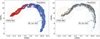 |
Fig. 1. Left: Two-dimensional UMAP representation of the TabPFN latent space for the FSRQs (red) and BL Lacs (blue) of the full FSRQ+BL Lac sample in the 4LAC-DR3 catalogue. Right: Same representation for the BCU sample. To better visualize the regions, ellipses have been overlaid to guide the eye through the latent space structure. |
Another important clarification concerns the interpretation of the latent space structure presented in Fig. 1. Before the application of the UMAP projection, the data were processed through a supervised classification model, namely TabPFN, trained using the source labels provided in the 4LAC-DR3 catalogue (as detailed in Appendix C). As a result, both the predicted probabilities and the intermediate embeddings produced by the model inherently reflect this supervised information. This setup naturally leads to a UMAP projection in which the latent space aligns with the BL Lac probability PBLL, leading to a smooth and continuous representation.
It is important to emphasize that the specific geometric shape observed in the UMAP projection of the latent space, which, in our case, is an arch-like structure, does not carry intrinsic physical meaning. This layout is a product of the UMAP algorithm’s initialization, and different parameter choices yield differently-shaped projections. What is meaningful, however, is the smooth correlation between the layout and the observational properties of the sources, such as the spectral index, the flux, the variability, etc. This correlation guarantees that our conclusions are driven by meaningful associations, rather than artifacts of the projection technique.
Looking through this continuous structure we observe an elongated region on the right, predominantly composed of BL Lacs (blue points), while FSRQs (red points) are mostly concentrated on the left. Between the BL-Lac dominated region (right) and the FSRQ-dominated region (left), we identify a third, intermediate region that can be distinguished from the two main populations. The dominant source type in this region is less clearly defined, and it may contain objects whose properties slightly deviate from both FSRQs and BL Lacs. These sources could potentially represent a transitional population between the two classes. A more comprehensive discussion on this transitional behaviour, incorporating all source types, is provided in Section 5. Interestingly, we observe that some FSRQs are located in the region dominated by BL Lacs and vice versa. This likely corresponds to originally misclassified sources in the catalogue. Finally, it is important to note that in Fig. 1, the UMAP dimensions (X and Y axes) do not carry direct physical meaning, as they only reflect the coordinates of each source in the reduced-dimensional space.
Finally, we fixed the two-dimensional UMAP mapping fitted on the 50-dimensional feature space of the FSRQs and BL Lacs, and applied this same transformation to all subsequent visualizations. Freezing this UMAP non-linear projection preserves a consistent relationship between the latent space and its two-dimensional representation, ensuring that all plots share the same geometric mapping. This consistency enables a reliable interpretation of the distribution of the sources in the latent space and facilitates a direct comparison between different blazar subsets.
4.2. The BCU population
At this step, we can visualize in the right panel of Fig. 1 the distribution of BCUs in the same latent space representation presented in Section 4.1. By comparing this to the left panel, where FSRQs and BL Lacs are found in opposite regions of the latent space, we observe that some BCUs fall within the regions dominated by either FSRQs (left) or BL Lacs (right). However, a significant fraction lies in the intermediate zone, previously discussed in Section 4.1, where the dominant class is not well defined. This spatial overlap suggests a dual nature of the BCU population: some can be reliably associated with one of the two known classes, while others may possess hybrid or atypical characteristics that prevent a straightforward classification. This indicates that some BCUs exhibit properties shared between FSRQs and BL Lacs, making their classification more challenging. Such intermediate characteristics could point to a transitional population, a possibility we examine more closely in the next section.
4.3. Population study
Once a probability PBLL (along with its associated uncertainty) was obtained for all sources, we used the UMAP-reduced dimensional latent space representation of TabPFN as a pivotal tool to explore the properties of the entire blazar population. This approach not only enables us to determine where BCUs lie in relation to FSRQs and BL Lacs, but also to characterize all sources in our sample, thereby gaining deeper insight into potential links between different types of blazars. To this end, we assign a BL Lac probability to all sources in the 4LAC-DR3.
We first visualize the latent space for the full blazar sample, comprising FSRQs, BL Lacs, and BCUs, colour-coded by their respective PBLL values. This representation allows us to evaluate how well the model captures a continuum between the two main classes. As shown in Fig. 2, the two extremes arewell-separated, with FSRQ-like sources having PBLL < 0.2 and BL Lac-like sources with PBLL > 0.9. An intermediate population fall between these, within the interval 0.2 ≤ PBLL ≤ 0.9.
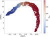 |
Fig. 2. Two-dimensional UMAP representation of the TabPFN latent space for the (FSRQ+BL Lac+BCU) blazar sample colour-coded by the probability PBLL. |
We then display the same latent space, this time coloured according to the source type (Fig. 3). Similarly to the left panel of Fig. 1, we identify on the left the region dominated by FSRQ-like sources. When considering the full blazar sample, this includes both Fermi-classified FSRQs (red) and BCUs with PBLL < 0.2 (orange). On the right, we retrieve the region dominated by BL Lac-like sources, consisting of Fermi BL Lacs (dark blue) and BCUs with PBLL > 0.9 (light blue). In contrast, sources falling within the probability range 0.2 ≤ PBLL ≤ 0.9 and located in the intermediate region are a mix of FSRQs, BL Lacs, and BCUs. This suggests a heterogeneous group whose properties blend those of FSRQs and BL Lacs.
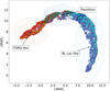 |
Fig. 3. Two-dimensional UMAP representation of the TabPFN latent space for the full blazar sample including FSRQs (red), FSRQ-like BCUs with PBLL < 0.2 (orange), BL Lacs (dark blue), BL Lac-like BCUs with PBLL > 0.9 (light blue), and BCUs with 0.2 ≤ PBLL ≤ 0.9 (green). |
This visualization indicates that the conventional FSRQ versus BL Lac classification holds primarily for extreme cases (e.g., HSP BL Lacs vs. FSRQs), but may require refinement in the intermediate region, where objects with mixed or evolving properties dominate. The presence of this intermediate region supports the concept of CLBs, as proposed in recent studies (e.g. Kang et al. 2024).
It is important to emphasize that our study focuses on a slow, long-term evolutionary scenario, consistent with the interpretation proposed by Kang et al. (2024). In this framework, CLBs correspond to FSRQs that gradually evolve towards a BL Lac state through a progressive decrease in accretion efficiency, potentially entering the ADAF regime over cosmological timescales. As such, our definition of CLBs excludes cases like OQ 334, which are characterized by rapid and reversible state changes on timescales of days to months (as previously discussed in the introduction). Accordingly, throughout this work, we adopt the terminology of Kang et al. (2024) and refer to the sources located in the intermediate region of our latent space as CLBs.
To deepen our understanding of this transition, we next provide complementary visualizations of the same latent space, in which points are colour-coded by additional physical properties. We first use the SED information, which specifies the position of the synchrotron peak when available. As shown at the bottom right of Fig. 4, we observe, as expected, that the left region, dominated by FSRQ-like objects, consists primarily of LSP sources. On the right, it is clear that HSP BL Lacs occupy the lower part of the BL Lac region, with a transition through ISP to LSP BL Lacs in the upper part. Interestingly, in the transition region, the CLBs tend to be LSP-like, which aligns with their intermediate position between FSRQs and LSP BL Lacs in Fig. 3. Then, we use the features that were most important for discriminating FSRQs from BL Lacs in our model. As shown in Fig. B.1, these include the synchrotron peak frequency (nu_syn) and the high-energy photon index (PL_Index), both of which are closely tied to the physical nature of the sources. The reduced latent space coloured by these features is presented in the top left and top right panels of Fig. 4. These visualizations confirm keytrends :
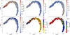 |
Fig. 4. Two-dimensional UMAP representation of the latent space for the full 4LAC-DR3 sample, colour-coded with the high-energy photon index PL_Index (top left), Variability_Index (top middle) the frequency of the synchrotron peak nu_syn (top right), the detection significance Signif_Avg (bottom left), the redshift z (bottom middle) and the SED_class (bottom right). For better visibility, missing values of the redshift (z) and of the synchrotron peak (nu_syn) are not displayed. |
-
FSRQ-like sources are located in a region with low log10(nu_syn) < 13 and soft spectra (PL_Index > 2.4).
-
Conversely, BL Lac-like sources are found in areas with high log10(nu_syn) > 16 and hard spectra (PL_Index < 2).
-
CLBs occupy a transitional zone, with intermediate values: 13 < log10(nu_syn) < 15 and 2 < PL_Index < 2.4.
It is important to emphasize that the intermediate values of the photon index PL_Index observed for CLBs are not an artifact of limited detection significance. As shown in the bottom left panel of Fig. 4, the average detection significance (Signif_Avg) appears to be smoothly distributed across the latent space, without being confined to a specific region. This suggests that the intermediate PL_Index values found in the transition region genuinely reflect intrinsic physical properties of these sources, rather than being driven by observational biases.
Interestingly, we also identify a distinct branch in the latent space associated with sources exhibiting higher Signif_Avg values. As shown in the top middle panel of Fig. 4, this branch corresponds to highly variable sources. By examining Fig. 3, we note that this region is primarily populated by non-BCU sources, suggesting that BCUs in the 4LAC-DR3 generally exhibit lower levels of variability.
Another key feature for investigating source properties is the redshift z. As mentioned in Section 2, FSRQs are generally found at higher redshift than BL Lacs, a trend well documented in recent blazar catalogues like the 4LAC-DR3 (Ajello et al. 2022). When colouring the latent space with the redshift (bottom middle panel of Fig. 4), this trend is indeed recovered: high-redshift sources are concentrated on the left region (dominated by FSRQs), while low-redshift sources are found on the right (dominated by BL Lacs). However, the transition between these regions is less evident, likely due to incomplete redshift data making it difficult to fully resolve a continuous distribution.
To further investigate this transition and better characterize the redshift distribution of each population, we divided the continuous PBLL distribution into three intervals, using the thresholds defined in Appendix C.1: (i) PBLL < 0.2, (ii) 0.2 ≤ PBLL ≤ 0.9, and (iii) PBLL > 0.9.
The goal was to assess whether we can distinguish three distinct groups: high-redshift FSRQs, low-redshift BL Lacs, and an intermediate group potentially corresponding to CLBs. The results are shown in Fig. 5 using the KDE algorithm.
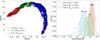 |
Fig. 5. Left: Two-dimensional UMAP representation of the latent space for the full 4LAC-DR3 sample split into PBLL bins. Right: Corresponding redshift density distributions. The shaded regions represent high-density intervals based on a KDE. |
It is important to note that the shaded regions do not represent formal confidence intervals. Instead, they correspond to high-density intervals centred around the peak values of the distributions, as defined using a KDE approach. This method is well suited to account for potentially broad or asymmetric distribution shapes, and it helps to better visualize and interpret the results. The redshift distributions indeed reveal three distinguishable populations:
-
FSRQs (PBLL < 0.2): mean redshift ⟨z⟩ = 1.25, with a high-density interval of [0.59, 1.90].
-
BL Lacs (PBLL > 0.9): ⟨z⟩ = 0.40, with [0.03, 0.77].
-
CLBs (0.2 ≤ PBLL ≤ 0.9): ⟨z⟩ = 0.79, with [0.20, 1.40].
While CLBs do occupy an intermediate range of redshift, their distribution is flatter and overlaps with both the FSRQ and BL Lac distributions, making them less sharply defined. Nonetheless, this result aligns with the findings of Kang et al. (2024), where CLBs also appear at intermediate redshift, supporting the hypothesis of a cosmological evolution from FSRQs to BL Lacs.
Furthermore, their study reported a similar transition in the photon index, moving from soft FSRQ spectra to hard BL Lac spectra through intermediate values for CLBs. This trend is consistent with the 4LAC-DR3 results (see Ajello et al. 2022, Fig. 1) where three distinct populations of photon index (corresponding to FSRQs, BCUs, and BL Lacs) were noted. We expand on this aspect in Fig. 6, where we show the density distributions of PL_Index and other meaningful features across the three PBLL bins. As expected, since PL_Index is the most discriminative feature for the model, we observe in the top left panel of Fig. 6 three well-separated populations in terms of photon index, with a value of PL_Index centred around 2.3 for CLBs. Similar patterns appear in the distributions of Pivot_energy (top right panel) and HE_EPeak (bottom right panel). Although the distinction in nu_syn (bottom left panel) is less pronounced, likely due to the high rate of missing data, the overall trend remains consistent: CLBs exhibit intermediate values between FSRQs and BL Lacs.
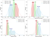 |
Fig. 6. PL_Index, Pivot_energy, nu_syn and HE_EPeak density distributions for different PBLL bins. |
These results, together with the gradual evolution of the source classification based on the SED properties, as illustrated in the bottom right panel of Fig. 4, support a scenario in which CLBs represent an intermediate evolutionary phase within a continuous transition from FSRQs to BL Lac objects. In this transition, sources progress through the sequence: FSRQ → CLB → LSP BL Lac → ISP BL Lac → HSP BL Lac, reflecting a gradual shift from low- to high-synchrotron-peaked SEDs. Their physical properties, across both SED features and gamma-ray spectra, suggest that their accretion disks are not yet fully depleted, but are evolving towards a radiatively inefficient state. The transition we find is consistent with evolutionary models of blazars where the gradual depletion of the circumnuclear material leads to changes in the accretion regime (Cavaliere & D’Elia 2002; Boettcher & Dermer 2002). In the early stages, FSRQs are fuelled by gas-rich environments that allow high accretion rates and luminous, radiatively efficient disks (Yuan & Narayan 2014; Prandini & Ghisellini 2022). Over cosmic time, the reservoir of gas diminishes, accretion weakens, and the sources transition into the BL Lac population. In this framework, the sources in the transition region of the latent space are likely undergoing this shift, from efficient to inefficient accretion. This scenario naturally explains the continuous evolution of observational properties such as spectral indices, emission line strengths, and SED peak locations. If the depletion is driven by AGN feedback mechanisms or galaxy mergers, these processes could also regulate the timescales of the transition(Fabian 2012).
4.4. Towards a cosmological evolution: The central engine
Finally, in the context of the evolutionary scenario proposed by Cavaliere & D’Elia (2002) and Boettcher & Dermer (2002), if FSRQs evolve towards a radiatively inefficient accretion regime, characteristic of BL Lacs, such evolution should also be reflected in the physical properties of the central engine.
To investigate this aspect, Kang et al. (2024) made use of the catalogue of central engine properties for Fermi blazars compiled by Paliya et al. (2021). As mentioned in Section 2, this catalogue provides key parameters such as the black hole mass (MBH), the logarithm of the accretion disk luminosity (logLd) and the Compton dominance (CD), defined as the ratio between the inverse Compton and synchrotron peak luminosities, an indicator of the relative strength of the high-energy emission. Their analysis reveals that CLBs lie in an intermediate region of the feature space concerning both logLd and CD, supporting the idea of a gradual transition in accretion properties. However, no such trend was found for MBH, suggesting that black hole mass alone may not play a primary role in driving this evolution.
Building on these results, we present in Fig. 7 our reduced latent space representation coloured by logLd and CD. Additionally, we further applied a logarithmic transformation to logLd and CD to better highlight differences between populations in the reduced latent space. Prior to this transformation, we ensured that only strictly positive values of logLd and CD were retained, to avoid undefined or non-physical values. These maps clearly show a distinction between FSRQs, characterized by high logLd and CD values on the left side of the latent space, and BL Lacs, which exhibit significantly lower values and dominate the right region. This is consistent with the physical interpretation that FSRQs harbour radiatively efficient accretion disks and strong external photon fields, resulting in a more prominent inverse Compton component. We note that in the FSRQ-dominated region of the latent space, a few sources show lower-than-average values of CD and logLd. This may reflect a transitional phase, where the accretion disk and external photon fields are fading, reducing both observables while the source still displays broad optical lines and is thus classified as an FSRQ. Misclassification may also contribute: as shown in Fig. C.2, a small fraction of BL Lacs in the 4LAC catalogue have a low BL Lac probability (PBLL < 0.2) and fall within the FSRQ region. These represent only about 1% of the total, and thus have minimal impact on the overall interpretation. As in previous sections, we further investigated this transition by displaying the density distributions of logLd and CD across the three PBLL bins, as shown in Fig. 8. These distributions again reveal a continuoustransition between FSRQs and BL Lacs, with CLBs occupying the intermediate regime. To better visualize the central trend, we also report the mean of logLd and CD in logarithmic units. The resulting average values in log scale are ⟨log10(logLd)⟩ = 1.65 and ⟨log10(CD)⟩ = 0.44, reinforcing the classification of CLBs as a transitional population in terms of central engine activity.
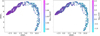 |
Fig. 7. Two-dimensional latent space representation of the full blazar sample, colour-coded by logLd (left panel) and CD (right panel). The missing values are not shown. |
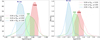 |
Fig. 8. logLd and CD density distributions for different PBLL bins. |
Together with the results in Section 4.3, which showed similar transitions in redshift and photon index, these findings further support a scenario in which blazars evolve from FSRQs to BL Lacs via an intermediate CLB phase. Initially, young FSRQs possess high accretion rates and standard thin accretion disks, producing strong emission lines. Over time, as their gas reservoir depletes, they transition into CLBs with intermediate accretion properties, eventually becoming BL Lacs, whose central engines are characterized by low accretion rates and radiatively inefficient flows, such as ADAFs (Yuan & Narayan 2014; Prandini & Ghisellini 2022).
In this work, we not only confirm the trends reported in Kang et al. (2024), but also introduce a unified latent representation that allows for a direct and intuitive visualization of the blazar evolutionary sequence. This latent space framework, combined with the inferred probability PBLL, provides a powerful tool to track the progressive changes in both jet and central engine properties across the blazar population.
5. Discussion
5.1. A new way of characterizing blazars
Based on these results and our latent space representation, we propose an alternative framework for characterizing blazars. Instead of assigning a discrete class label, each source can be described using two complementary and continuousdescriptors:
-
Its probability PBLL of being a BL Lac.
-
Its position in the UMAP-projected latent space of the TabPFN model.
By combining these two pieces of information, we move beyond rigid binary classification and enable a more flexible, interpretable, and physically motivated description of the blazar population. This approach is particularly well suited for sources with ambiguous or intermediate properties, such as BCUs or, more generally, CLBs, and can be directly applied to future releases of blazar catalogues.
Furthermore, this framework allows for an intuitive exploration of blazar evolution. By colour-coding the latent space with key features (e.g., spectral indices, accretion-related quantities), users can easily investigate the progressive transition from FSRQs to BL Lacs, with CLBs forming an intermediate bridge. This visual exploration can be enriched with histograms (see Section 4.4) to define typical parameter ranges across the transition. In light of these findings, we propose a unified visualization of blazar evolution, shown in Fig. 9. Each evolutionary phase, discretized into three bins of PBLL, is associated with characteristic ranges for the most discriminating features. These include the gamma-ray photon index, redshift, accretion disk luminosity, and Compton dominance, which act as proxies for the underlying physical processes driving the transition from FSRQs to BL Lacs. This representation constitutes a significant step towards a unified scheme of blazar evolution. It offers a data-driven and interpretable framework for the understanding of the diversity in the blazar population and their potential evolutionaryconnection.
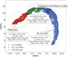 |
Fig. 9. Unified representation of blazar evolution. The continuous UMAP representation of the TabPFN latent space has been divided into three bins of PBLL, corresponding to the three potential evolutionary phases. For each phase, we provide the characteristic ranges for the most discriminating features. These ranges represent high-density intervals around the KDE peaks identified in the histograms presented in previous sections. |
Finally, to strengthen our results, we included a sample of CLB candidates identified in
Kang et al. (2025). In that study, the authors built upon their previous work
(Kang et al. 2024), where CLBs were defined as sources showing intermediate values in key physical parameters such as the Compton dominance, the accretion disk luminosity, and the redshift.
In their follow-up analysis, Kang et al. (2025) applied an unsupervised clustering algorithm to these parameters and identified four optimal combinations that could effectively separate FSRQs, BL Lacs, and CLBs. They compiled a catalogue that includes the original classification from Kang et al. (2024) alongside the clustering results for the four parametercombinations.
To ensure consistency with the gradual evolutionary scenario proposed in Kang et al. (2024), we selected only the sources that were: (i) classified as CLBs in the original study, and (ii) consistently identified as CLB candidates (CLBCs) in all four clustering combinations of Kang et al. (2025). The resulting sample consists of 42 blazars, which we display in our latent space projection (Fig. 10).
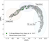 |
Fig. 10. Two-dimensional UMAP representation of the TabPFN latent space showing a subset of CLBCs from Kang et al. (2025), highlighted in green. All other sources in the sample are shown in grey. The clustering of CLBCs in the intermediate region supports the interpretation of this zone as a transitional phase between FSRQ-like and BL Lac-like states. |
We observe that the majority of CLBCs from Kang et al. (2024, 2025) fall within, or very close to, the intermediate region of our reduced latent space. This observation supports our interpretation that this region corresponds to a transitional phase, where sources evolve gradually from an FSRQ-like state towards a BL Lac-like state.
A smaller fraction of CLBCs are found outside this region, primarily in the area dominated by FSRQs. This is likely due to the overlap between the CLB and FSRQ clusters in the feature space of Kang et al. (2025) (see Fig. 5 therein), indicating that some sources classified as CLBs still share characteristics with the FSRQ population.
Overall, the spatial consistency between our latent space representation and the independently identified CLBCs provides strong support for the validity of our approach. It confirms the ability of the latent representation to reflect meaningful evolutionary trends within the blazar population, and demonstrates its potential as a powerful framework to identify and investigate sources undergoing, or susceptible to undergo, long-term transitions between blazar subclasses.
5.2. A tool for investigating missing data
An additional and particularly compelling application of the reduced latent space representation is its potential to provide insights into missing data. As illustrated at the bottom right of Fig. 4, we overlaid the regions where the SED_class information, available in the 4LAC-DR3 catalogue, is missing. Interestingly, the spatial coherence in the distribution of sources with known SED classes suggests that their neighbours in latent space share similar physical properties. This implies that the latent space serves as a valuable proxy to infer likely values for missing observational quantities, such as the synchrotron peak position, the redshift, or even the black hole mass. While not a substitute for direct measurements, such inferences can offer useful priors or guide observational follow-ups. In this way, our latent representation becomes a powerful tool not only for classification and population studies but also for mitigating the impact of incomplete data in blazar catalogues.
6. Conclusions
In this study, we explored the application of the TabPFN model for blazar classification on a major dataset: the 4LAC-DR3 catalogue. The model was trained on well-identified sources (FSRQs and BL Lacs) and subsequently applied to BCUs, providing a more complete and probabilistic characterization of the blazar population. Our main findings can be summarized as follows:
-
The classification probabilities assigned by TabPFN are consistent with known blazar properties, revealing a smooth transition from FSRQs to BL Lacs, notably through an intermediate population of CLBs. This observation supports an evolutionary scenario in which blazars gradually evolve from FSRQs to HSP BL Lacs due to the depletion of circumnuclear material (Cavaliere & D’Elia 2002; Boettcher & Dermer 2002), as also suggested by Kang et al. (2024).
-
The use of the continuous probability score PBLL allows a flexible characterization of sources within the intermediate range 0.2 ≤ PBLL ≤ 0.9. This avoids rigid, pre-defined classification schemes (such as SED_class) and is further strengthened by bootstrap-based uncertainty estimates that quantify the reliability of each prediction.
-
Interestingly, CLBs consist of a heterogeneous mix of FSRQs, BL Lacs, and BCUs, most of which are LSP sources. This suggests that CLBs may retain FSRQ-like properties, such as a thin and efficient accretion disk, even during this transitional phase.
-
By segmenting the latent space based on PBLL, we uncover four distinct populations with respect to key physical properties: gamma-ray photon index, redshift, accretion disk luminosity, and Compton dominance. In each of these features, CLBs consistently occupy an intermediate regime, supporting the hypothesis of a continuous cosmological evolution from efficient to inefficient accretion.
-
This intermediate region is significantly populated by CLB candidates identified in recent studies (Kang et al. 2024, 2025), further validating the physical relevance of our latent space representation and reinforcing the robustness of our conclusions.
A central strength of our approach lies in the combination of the latent space representation and the scalar PBLL probability. This enables an insightful visualization of the relationship between blazar type and physical properties.
The latent representation provides a basis for inferring missing values, such as redshift or SED_class, by examining a source’s position within the continuous distribution of known observational properties. This could serve as a prior for sources with incomplete data.
Ultimately, we proposed a visualization-based framework that supports a possible unified evolutionary scheme for blazars, underscoring the power of combining machine learning with physical interpretation.
Nevertheless, it is important to note that uncertainties in feature measurements were not incorporated in the current implementation, as neither TabPFN nor UMAP natively accounts for uncertainties. Future work could implement this approach by incorporating observational errors with an updated method, by applying our current method to other blazar catalogues, and by integrating complementary data into our current approach (e.g., spectroscopic redshift, polarization, or variability measurements). These enhancements would provide even stronger constraints on the proposed evolutionary scenario from FSRQs to BL Lacs via CLBs.
Of particular interest, and to the best of our knowledge, this work represents the first application of a pre-trained foundation model for tabular data to the field of high-energy astrophysics. We showcased the strength of this approach, which requires no model-specific training or optimization, apart from minimal hyper-parameter tuning, and which yet provides fast and interpretable results.
In conclusion, this study demonstrates how modern deep learning models, such as TabPFN, when guided by astrophysical understanding, can offer powerful new ways to explore the nature and evolution of blazars.
Acknowledgments
The authors acknowledge the support provided by Université Paris Cité to Prof. Yvonne Becherini through the Chaire Professorale IdEX, as well as support from the Data Intelligence Institute of Paris (diiP) at Université Paris Cité. We also thank Maximilian Eff for carefully reading the final manuscript and offering valuable feedback. We thank the anonymous referee for the useful comments, which helped clarify some concepts in the paper. Minor language edits were assisted by AI tools.
References
- Abdo, A. A., Ackermann, M., Ajello, M., et al. 2009, ApJ, 716, 30 [Google Scholar]
- Abdollahi, S., Acero, F., Ackermann, M., et al. 2020, ApJS, 247, 33 [Google Scholar]
- Abdollahi, S., Acero, F., Baldini, L., et al. 2022, ApJS, 260, 53 [NASA ADS] [CrossRef] [Google Scholar]
- Agarwal, A. 2023, ApJ, 946, 109 [Google Scholar]
- Ajello, M., Baldini, L., Ballet, J., et al. 2022, ApJS, 263, 24 [NASA ADS] [CrossRef] [Google Scholar]
- Akiba, T., Sano, S., Yanase, T., Ohta, T., & Koyama, M. 2019, in Proceedings of the 25th ACM SIGKDD International Conference on Knowledge Discovery& Data Mining, 2623 [Google Scholar]
- Bhatta, G., Gharat, S., Borthakur, A., & Kumar, A. 2024, MNRAS, 528, 976 [Google Scholar]
- Boettcher, M., & Dermer, C. D. 2002, ApJ, 564, 86 [CrossRef] [Google Scholar]
- Böttcher, M. 2006, Astrophys. Space Sci., 309, 95 [Google Scholar]
- Böttcher, M., Reimer, A., & Sweeney, K. 2013, ApJ, 768, 54 [NASA ADS] [CrossRef] [Google Scholar]
- Breiman, L. 2001, Mach. Learn., 45, 5 [Google Scholar]
- Cavaliere, A., & D’Elia, V. 2002, ApJ, 571, 226 [NASA ADS] [CrossRef] [Google Scholar]
- Chen, T., & Guestrin, C. 2016, in Proceedings of the 22nd ACM SIGKDD International Conference on Knowledge Discovery and Data Mining, 785 [Google Scholar]
- Cortes, C., & Vapnik, V. 1995, Mach. Learn., 20, 273 [Google Scholar]
- Fabian, A. C. 2012, ARA&A, 50, 455 [Google Scholar]
- Ghisellini, G., Tavecchio, F., Foschini, L., & Ghirlanda, G. 2011, MNRAS, 414, 2674 [NASA ADS] [CrossRef] [Google Scholar]
- Giommi, P., & Padovani, P. 2015, MNRAS, 450, 2404 [Google Scholar]
- Hollmann, N., Müller, S., Eggensperger, K., & Hutter, F. 2023, in International Conference on Learning Representations (ICLR) [Google Scholar]
- Hollmann, N., Müller, S., Purucker, L., et al. 2025, Nature, 637, 319 [CrossRef] [Google Scholar]
- Hornik, K., Stinchcombe, M., & White, H. 1989, Neural Networks, 2, 359 [CrossRef] [Google Scholar]
- Kang, S.-J., Zheng, Y.-G., & Wu, Q. 2023, MNRAS, 525, 3201 [NASA ADS] [CrossRef] [Google Scholar]
- Kang, S.-J., Lyu, B., Wu, Q., Zheng, Y.-G., & Fan, J. 2024, ApJ, 962, 122 [NASA ADS] [CrossRef] [Google Scholar]
- Kang, S., Ren, S., Zheng, Y., & Wu, Q. 2025, ApJ, 980, 122 [Google Scholar]
- Mahesh, T. R., Vinoth Kumar, V., Dhilip Kumar, V., et al. 2023, Patterns, 4, 100835 [Google Scholar]
- Massaro, E., Maselli, A., Leto, C., et al. 2015, Astrophy. Space Sci., 357, 75 [Google Scholar]
- McInnes, L., Healy, J., Saul, N., & Großberger, L. 2018, J. Open Source Software, 3, 861 [CrossRef] [Google Scholar]
- Mingaliev, M., Sotnikova, Y., Mufakharov, T., Erkenov, A. K., & Udovitskiy, R. Y. 2015, Astrophys. Bull., 70, 264 [Google Scholar]
- Padovani, P., & Giommi, P. 1995, ApJ, 444, 567 [NASA ADS] [CrossRef] [Google Scholar]
- Paliya, V. S., Domínguez, A., Ajello, M., Olmo-García, A., & Hartmann, D. 2021, ApJS, 253, 46 [NASA ADS] [CrossRef] [Google Scholar]
- Prandini, E., & Ghisellini, G. 2022, Galaxies, 10, 35 [NASA ADS] [CrossRef] [Google Scholar]
- Prokhorenkova, L., Gusev, G., Vorobev, A., Dorogush, A. V., & Gulin, A. 2018, in Advances in Neural Information Processing Systems, 31 [Google Scholar]
- Ren, S. S., Zhou, R. X., Zheng, Y. G., Kang, S. J., & Wu, Q. 2024, A&A, 685, A140 [NASA ADS] [CrossRef] [EDP Sciences] [Google Scholar]
- Ricci, C., & Trakhtenbrot, B. 2023, Nat. Astron., 7, 1282 [Google Scholar]
- Sahakyan, N., Vardanyan, V., & Khachatryan, M. 2022, MNRAS, 519, 3000 [Google Scholar]
- Shakura, N. I., & Sunyaev, R. A. 1973, A&A, 24, 337 [NASA ADS] [Google Scholar]
- Sklearn 2025, Model Evaluation, scikit-learn 1.4.2 documentation, https://scikit-learn.org/stable/modules/model_evaluation.html [Google Scholar]
- Urry, C. M., & Padovani, P. 1995, Publ. Astron. Soc. Pac., 107, 803 [NASA ADS] [CrossRef] [Google Scholar]
- Yuan, F., & Narayan, R. 2014, ARA&A, 52, 529 [NASA ADS] [CrossRef] [Google Scholar]
Appendix A: Feature visualization
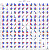 |
Fig. A.1. Visual representation of the feature space for the key 4LAC-DR3 parameters. A log10 transformation is applied. Missing values are not shown. |
Appendix B: Training strategy and optimization
B.1. Data split and cross-validation
For our dataset (4LAC-DR3), we initially divided the samples into two subsets: one subset, containing only FSRQs and BL Lacs, used for training and testing, and another subset, consisting solely of BCUs, reserved for subsequent predictions. Thus, the dataset of FSRQs and BL Lacs was used to train models for this classification end, based on their physical properties. Once trained, the models can then be applied to unseen data (the BCU sample) to classify uncertain blazars. A straightforward approach to training these models is to split the FSRQ and BL Lac dataset into two subsets: a training set, typically comprising 80% of the data, used to learn patterns, and a test set, consisting of the remaining 20%, used to evaluate the model’s performance. However, evaluating performance on a single test set might not adequately represent the entire dataset. This approach can introduce significant variability in results and produce models that fail to generalize well, increasing the risk of over-fitting.
To ensure robust training and evaluation, we employed cross-validation, a widely used technique in machine learning that involves training and testing a model multiple times on different subsets of the data. In our study, we used a method called Stratified K-Fold Cross-Validation (Mahesh et al. 2023) to reliably evaluate our models. This involves dividing the data into K equal parts. The model is trained on K − 1 parts and then tested on the remaining part. We repeated this process K times, each time testing on a different part. Finally, the overall performance is calculated by averaging the results from all K tests. Unlike standard K-Fold cross-validation, Stratified K-fold Cross-Validation ensures that class proportions are maintained across all folds. This is particularly useful in our case, as in 4LAC-DR3, BL Lacs (1458) are more numerous than FSRQs (792). As we describe in the next sections, cross-validation is crucial not only for evaluating classification performance but also for the optimization of the model parameters (in a procedure called hyper-parameter tuning) and for the selection of the most relevant features for classification.
B.2. Data preparation through feature optimization
Before obtaining the final classification results, it is crucial to refine the dataset by removing features that do not significantly help in classifying FSRQs and BL Lacs. Optimizing the dataset offers several advantages. Firstly, using a smaller set of relevant features helps the model to make better predictions by avoiding the possible memorization of irrelevant details (over-fitting), which improves accuracy on new data. Secondly, it makes the results easier to understand and explain, since fewer and more meaningful features provide clearer insights into the relation between the input and the output. Finally, it speeds up the analysis: fewer features mean lower memory usage and faster computations. For instance, in XGBoost, this results in fewer splits in decision trees, resulting in faster execution.
In this section, we present the data preparation process for the training task. This includes:
-
Simple feature engineering, transforming raw data into meaningful features to optimize learning.
-
Feature scaling, which standardizes features to ensure that they contribute equally to the model.
-
Feature importance evaluation, by using permutation methods coupled with cross-validation to assess the significance of each feature in predicting the target variable.
When dealing with features that span multiple orders of magnitude, like in our case, a log10 transformation can be an effective preprocessing step. This transformation compresses the scale of variables with wide ranges, reducing the influence of outliers while preserving the relative relationships between values. Therefore, to mitigate skewness and potentially improve the classification performance, a log10 transformation was applied to all features. Note that the log10 transformation, implemented using numpy, was applied only to numerical data, automatically ignoring missing values. During model training, missing values are explicitly converted to NaNs (“Not a Number”), allowing the classification algorithms to handle them appropriately within the learning process. After applying the logarithmic transformation, standardizing the data to have zero mean (μ = 0) and unit variance (σ = 1) further normalizes the features, ensuring they contribute equally to subsequent analyses or modelling techniques. This step ensures well-defined distributions closer to normality, which is essential for foundation models like TabPFN, as they have been pre-trained on normalized distributions (see Hollmann et al. 2023, Section C.2.1). However, tree-based models like XGBoost do not require such feature scaling approaches, as they inherently handle different feature scales, although applying them can sometimes improve convergence and stability. Therefore, we applied both transformations (logarithmic + standardization) for TabPFN, while for XGBoost, we only applied the log10 transformation.
To further evaluate the significance of our features, we applied a permutation importance method combined with cross-validation. The principle behind this method is to evaluate how much the model’s performance is affected when the values of a given feature are randomly shuffled. This process helps determine the contribution of each feature for the classification task: if the model performance drops, the feature is important, while if the performance remains unchanged, the feature is less relevant or redundant. To ensure stability, the permutation process was repeated multiple times averaging the results to obtain a robust estimate of feature importance. For XGBoost, this feature importance analysis was performed in parallel with stratified cross-validation across the full dataset. However, as mentioned in Section 3.1, TabPFN is designed to operate in a zero-shot manner, meaning it does not require multiple training iterations. Consequently, applying stratified cross-validation for feature optimization on TabPFN would result in high computational costs and long execution times, even with parallelization. To mitigate this, feature importance analysis for TabPFN was performed without cross-validation. This approach provides a sufficiently accurate estimation of the most relevant features for distinguishing FSRQs from BL Lacs, while maintaining computational efficiency.
Feature optimization results for the 4LAC-DR3, with TabPFN (top) and XGBoost (bottom), can be seen in Fig. B.1. Since we have an imbalanced dataset (FSRQs vs BL Lacs), the accuracy (percentage of correctly classified sources) is not the most reliable metric to evaluate classification performance. We therefore consider the following key metrics (see Sklearn 2025) that better reflect the model’s ability to distinguish between both source types:
-
Balanced accuracy which takes into account the accuracy for each class independently, providing a better evaluation in case of class imbalance.
-
ROC-AUC (receiver operating characteristic - area under the curve) measuring how well the model separates FSRQs from BL Lacs. It is based on the ROC curve, which plots the true positive rate (TPR) against the false positive rate (FPR). A ROC-AUC score of 0.5 means the model is making random guesses, while a score of 1 indicates a perfect classification.
-
F1-score that balances precision (how many of the sources classified as BL Lacs are truly BL Lacs) and recall (how many of the actual BL Lacs are correctly identified). It is particularly useful when dealing with imbalanced datasets, as it avoids misleadingly high performance due to majority class dominance.
B.3. Identifying key features in the 4LAC catalogue
Based on these metrics, we observe that the most relevant features for distinguishing FSRQs from BL Lacs in the 4LAC catalogue includes :
-
The spectral indices that represent the high-energy SED spectral behaviour, captured by the power-law and log-parabolic indices (PL_Index, LP_Index). These features separate the two classes by encoding distinctions in their gamma-ray spectral shapes.
-
The synchrotron peak which represents the synchrotron peak frequency (nu_syn) and reflects the difference in the jet emission physics.
-
The pivot energy which represents the reference energy (Pivot_energy) at which the gamma-ray spectral parameters are most tightly constrained. This feature serves as a reference energy, reflecting differences in the inverse Compton peak energies of FSRQs and BL Lacs. FSRQs typically exhibit lower pivot energies, while BL Lacs often show higher pivot energies.
-
The source variability which represents the flux variability of the source (quantified by Variability_Index) and often offers supplementary discriminative power.
It is worth noting that both models account for potential correlations between features. In the case of TabPFN, this is handled during the pre-training phase through a technique called block-wise feature sampling, where adjacent features are grouped to reflect the correlated behaviour observed in the data. This approach allows for the inclusion of a wider range of features during the feature selection process without imposing restrictions on their correlation.
As shown in Fig. B.1, it appears that TabPFN assigns notable importance to a broader range of features than XGBoost. This is likely due to the fact that TabPFN is a more complex model, capable of capturing intricate relationships between features. Interestingly, while PL_Index consistently ranks among the most important features for distinguishing FSRQs from BL Lacs in both models, information related to the energy/flux of the inverse Compton peak appears to be less relevant. In contrast, features related to variability, the synchrotron peak, and the high-energy slope seem to play a more crucial role in classification.
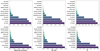 |
Fig. B.1. Feature importance results for different classification metrics (balanced_accuracy, roc_auc and f1) with TabPFN (top panel) and XGBoost (bottom panel). |
When using only the top key features, we observe an improvement across all evaluated metrics (balanced accuracy, ROC AUC, and F1 score). Consequently, we chose to retain the 8 most important features for each model, as shown in Fig. B.1. This decision is further supported by the fact that complex models like TabPFN tend to perform better when provided with a compact yet informative set of features, as they are capable of capturing intricate patterns in the feature space.
B.4. Fine-tuning model parameters
Once the data have been properly prepared, it is often crucial to fine-tune the parameters of the classification model, also known as hyper-parameters, in a process referred to as hyper-parameter optimization.
In the case of XGBoost, hyper-parameter tuning is essential. Since XGBoost is based on decision trees, it has numerous hyper-parameters that influence the performance and require careful optimization to achieve the best results. For example, the depth of the trees controls the complexity of the model, and adjusting this value helps in avoiding over-fitting (where an overly complex model memorizes the data instead of generalizing) or under-fitting (where the model is too simple to identify meaningful patterns). Similarly, key hyper-parameters such as the learning rate and the number of estimators regulate the learning process and its efficiency. Additionally, given the imbalanced nature of the dataset, adjusting the class weights during training helps to account for the fact that certain source types (e.g. BL Lacs) are overrepresented compared to others (e.g. FSRQs) in datasets like 4LAC-DR3.
On the other hand, TabPFN is fundamentally different from XGBoost, as it is based on pre-trained neural networks that make instantaneous predictions without requiring specific training on the blazar catalogues. As a result, hyper-parameter optimization is unnecessary, since TabPFN has already been optimized beforehand to adapt to a wide range of tabular datasets, considering different possible data distributions.
Consequently, we focused our hyper-parameter optimization efforts on XGBoost, using the Python library Optuna (Akiba et al. 2019). This tool explores the hyper-parameter space by testing different configurations, based on advanced Bayesian optimization methods. In parallel, we also performed cross-validation with 10 folds to ensure robust results. For each catalogue of blazars, we performed 100 trials with Optuna, leading to a selection of 10 hyper-parameters for tuning (including the number of estimators, max-depth, learning rate, and class weight), along with their optimal values. This optimization improves accuracy, as well as the roc_auc and F1 score metrics. One advantage of this method is that it automatically adjusts class weights, addressing the imbalance in the dataset.
As a side note, we can still apply hyper-parameter optimization in the case of TabPFN for 5 different parameters, including the n_estimators (the number of estimators in the TabPFN ensemble), softmax_temperature (which controls the confidence of the model’s predictions), and balance_probabilities (which adjusts the output probabilities to treat the classes as if they were equally likely).
Nevertheless, only slight performance differences were observed across these configurations, reflecting TabPFN’s overall robustness.
Appendix C: Testing the quality of the model
C.1. Performance on FSRQs versus BL Lacs
After selecting the most relevant features and optimizing the hyper-parameters to enhance the classification of FSRQs and BL Lacs, we proceeded to fit the models (XGBoost and TabPFN) on the training data. We then checked how well the model performed by testing it on different parts of the data, using ten-fold cross-validation. The performance of XGBoost and TabPFN are summarized in Table C.1. Both models perform exceptionally well, with TabPFN showing slightly better performance across the board. Key metrics like accuracy, precision, recall, and F1-score are consistent with those reported in Agarwal (2023) and Bhatta et al. (2024), which primarily relied on more traditional machine learning approaches. In contrast, our use of a foundation model (TabPFN) yields comparable performance while benefiting from its inherent ability to generalize and adapt across datasets without extensive hyper-parameter tuning.
Classification performance of XGBoost and TabPFN for the sample of FSRQs and BL Lacs in the 4LAC-DR3.
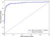 |
Fig. C.1. ROC curve obtained with the application of TabPFN to the sample of FSRQs vs BL Lacs in the 4LAC-DR3. |
Both models achieve AUC values exceeding 0.95, with TabPFN reaching 0.969. This result outperforms the AUC reported in recent works such as Agarwal (2023) and Bhatta et al. (2024), underlining the effectiveness of foundation models in tabular classification tasks involving complex astrophysical data. As mentioned previously, XGBoost was primarily used as a strong baseline to benchmark our foundation model. The results confirm that TabPFN consistently outperforms XGBoost, achieving higher accuracy and AUC scores.
To further assess TabPFN’s performance, we display Fig. C.1 the ROC curve which illustrates the model’s ability to distinguish between FSRQs and BL Lacs. The AUC score quantifies this performance: a value close to 1 indicates that the model is highly effective in separating the two classes. Additionally, Fig. C.2 shows the distribution of BL Lac classification probabilities (PBLL) as predicted by TabPFN. These probabilities were obtained for all sources in a test sample, consisting exclusively of BL Lacs and FSRQs.
In these plots, each bar represents several sources, with the colour corresponding to the true classification from the 4LAC catalogue. The X-axis indicates the predicted probability PBLL, which quantifies the likelihood of a source being classified as a BL Lac. A well-separated distribution with peaks near 0 and 1 suggests that the model confidently distinguishes between FSRQs and BL Lacs. High-density peaks are observed at both ends of the distribution, around PBLL = 0 (for FSRQs) and PBLL = 1 (for BL Lacs). Sources with PBLL near 0 correspond to the true FSRQs (as indicated by the red colour). Similarly, sources with PBLL close to 1 correspond to the true BL Lacs (as indicated by the blue colour). Only a small fraction of true BL Lacs is assigned a low PBLL, and conversely, only a small fraction of true FSRQs has a high PBLL. This result highlights TabPFN’s ability to correctly distinguish between the two classes. Notably, the performance reported in Table C.1, which is lower for the FSRQ class than for BL Lacs, is due to a higher proportion of misclassified FSRQs, as illustrated in Fig. C.2. These correspond to sources originally classified as FSRQs in the 4LAC catalogue but exhibiting observational properties identical to BL Lacs (i.e., a high PBLL value). Finally, we applied a KDE to the distribution of PBLL values in order to locate the probability density peaks associated with each population (kde_peak). This allowed us to define two classification thresholds: one above which sources are considered BL Lac-like, and another below which sources are considered FSRQ-like. To ensure that the thresholds remained close to the respective high-density peaks and avoid ambiguous cases near PBLL ∼ 0.5, we adopted a conservative criterion based on a small shift from the peak, defined as kde_peak ± 0.5 × std, where std is the standard deviation of the distribution around the peak. The resulting thresholds are shown in Fig. C.2, with a BL Lac-like threshold set at PBLL = 0.91 (blue dashed line) and a FSRQ-like threshold at PBLL = 0.19 (red dashed line) which we rounded to 0.9 and 0.2.
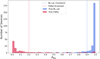 |
Fig. C.2. Distribution of BL Lac classification probabilities (PBLL) for all sources in the test set, as predicted by TabPFN. The X-axis represents PBLL, indicating the predicted probability of a source being a BL Lac, while the colour of each bar corresponds to its true classification in the catalogue. The dashed vertical lines indicate the thresholds derived from the KDE analysis, marking regions where sources are most confidently identified as either BL Lac-like (PBLL > 0.9) or FSRQ-like (PBLL < 0.2). |
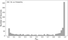 |
Fig. C.3. Distribution of BL Lac classification probabilities (PBLL) for all BCUs, as predicted by TabPFN. The predictions were obtained using a bootstrap method with 50 instances of TabPFN trained on different subsets of the data. |
C.2. Application on BCUs
After optimizing TabPFN on the FSRQ/BL Lac subsets of the 4LAC-DR3 catalogue, we applied the model to classify BCUs. Fig. C.3 shows the distributions of the predicted BL Lac probability, PBLL, for these BCUs. As in Section C.1, many predictions cluster near 0 or 1, suggesting that the model can efficiently classify a significant proportion of BCUs as either FSRQs or BL Lacs.
To quantify the reliability of these predictions, we estimated uncertainties via an ensemble approach. Specifically, we generated 50 bootstrapped training sets (resampling data with replacement) and trained a separate TabPFN instance, each with a unique random initialization, on each data sample. For every BCU, we then averaged its 50 probability estimates (⟨PBLL⟩) and computed their standard deviation as an uncertainty measure. The probability distribution in Fig. C.3 was obtained using this method, aggregating predictions from 50 TabPFN models trained on different data subsets. This approach helps us estimating how much predictions can vary without relying on strict assumptions about the error distribution. Therefore by simulating different training scenarios, we can estimate the uncertainty in the predictions. This approach is particularly valuable for methods like TabPFN, which does not provide explicit Bayesian-style uncertainty estimates out of the box.
To further analyse these uncertainties, we plot them as a function of the averaged predicted probabilities (⟨PBLL⟩) in Fig. C.4. A parabolic fit is overlaid to highlight the general trend. As expected, the highest uncertainties occur when the predicted probability is close to 0.5. This is because sources with a probability near 50% of being a BL Lac (PBLL ≈ 0.5) also have an equal probability (1–0.5 = 50%) of being an FSRQ. Such cases indicate that, based on their physical properties, the model struggles to confidently classify them as either type. In particular, we observe that a significant number of BCUs exhibit uncertainties greater than 25% when their predicted BL Lac probability is close to 50%. These outliers may represent a transitional class between FSRQs and BL Lacs, exhibiting properties that slightly deviate from both categories. To further highlight the classification reliability, a red box has been drawn around BCUs with a low probability of being BL Lac (PBLL < 0.2), meaning they are most likely FSRQs. Conversely, a blue box encloses BCUs with a high probability of being BL Lacs (PBLL > 0.8). These boxes also account for uncertainties by including only sources with prediction uncertainties below 0.1. Therefore, to study BCUs that closely resemble either FSRQs or BL Lacs, we focused on the sources within these respective boxes, while avoiding those located outside of them, as they exhibit greater classification ambiguity.
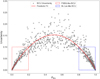 |
Fig. C.4. Average bootstrap BL Lac probabilities versus associated uncertainties for 4LAC-DR3 BCUs. A parabolic fit is overlaid to emphasize the trend and highlight potential outliers. The red and blue boxes enclose BCU sources with a high probability of being FSRQ and BL Lac, respectively, both exhibiting low uncertainty. |
All Tables
Classification performance of XGBoost and TabPFN for the sample of FSRQs and BL Lacs in the 4LAC-DR3.
All Figures
|
Fig. 1. Left: Two-dimensional UMAP representation of the TabPFN latent space for the FSRQs (red) and BL Lacs (blue) of the full FSRQ+BL Lac sample in the 4LAC-DR3 catalogue. Right: Same representation for the BCU sample. To better visualize the regions, ellipses have been overlaid to guide the eye through the latent space structure. |
| In the text | |
|
Fig. 2. Two-dimensional UMAP representation of the TabPFN latent space for the (FSRQ+BL Lac+BCU) blazar sample colour-coded by the probability PBLL. |
| In the text | |
|
Fig. 3. Two-dimensional UMAP representation of the TabPFN latent space for the full blazar sample including FSRQs (red), FSRQ-like BCUs with PBLL < 0.2 (orange), BL Lacs (dark blue), BL Lac-like BCUs with PBLL > 0.9 (light blue), and BCUs with 0.2 ≤ PBLL ≤ 0.9 (green). |
| In the text | |
|
Fig. 4. Two-dimensional UMAP representation of the latent space for the full 4LAC-DR3 sample, colour-coded with the high-energy photon index PL_Index (top left), Variability_Index (top middle) the frequency of the synchrotron peak nu_syn (top right), the detection significance Signif_Avg (bottom left), the redshift z (bottom middle) and the SED_class (bottom right). For better visibility, missing values of the redshift (z) and of the synchrotron peak (nu_syn) are not displayed. |
| In the text | |
|
Fig. 5. Left: Two-dimensional UMAP representation of the latent space for the full 4LAC-DR3 sample split into PBLL bins. Right: Corresponding redshift density distributions. The shaded regions represent high-density intervals based on a KDE. |
| In the text | |
|
Fig. 6. PL_Index, Pivot_energy, nu_syn and HE_EPeak density distributions for different PBLL bins. |
| In the text | |
|
Fig. 7. Two-dimensional latent space representation of the full blazar sample, colour-coded by logLd (left panel) and CD (right panel). The missing values are not shown. |
| In the text | |
|
Fig. 8. logLd and CD density distributions for different PBLL bins. |
| In the text | |
|
Fig. 9. Unified representation of blazar evolution. The continuous UMAP representation of the TabPFN latent space has been divided into three bins of PBLL, corresponding to the three potential evolutionary phases. For each phase, we provide the characteristic ranges for the most discriminating features. These ranges represent high-density intervals around the KDE peaks identified in the histograms presented in previous sections. |
| In the text | |
|
Fig. 10. Two-dimensional UMAP representation of the TabPFN latent space showing a subset of CLBCs from Kang et al. (2025), highlighted in green. All other sources in the sample are shown in grey. The clustering of CLBCs in the intermediate region supports the interpretation of this zone as a transitional phase between FSRQ-like and BL Lac-like states. |
| In the text | |
|
Fig. A.1. Visual representation of the feature space for the key 4LAC-DR3 parameters. A log10 transformation is applied. Missing values are not shown. |
| In the text | |
|
Fig. B.1. Feature importance results for different classification metrics (balanced_accuracy, roc_auc and f1) with TabPFN (top panel) and XGBoost (bottom panel). |
| In the text | |
|
Fig. C.1. ROC curve obtained with the application of TabPFN to the sample of FSRQs vs BL Lacs in the 4LAC-DR3. |
| In the text | |
|
Fig. C.2. Distribution of BL Lac classification probabilities (PBLL) for all sources in the test set, as predicted by TabPFN. The X-axis represents PBLL, indicating the predicted probability of a source being a BL Lac, while the colour of each bar corresponds to its true classification in the catalogue. The dashed vertical lines indicate the thresholds derived from the KDE analysis, marking regions where sources are most confidently identified as either BL Lac-like (PBLL > 0.9) or FSRQ-like (PBLL < 0.2). |
| In the text | |
|
Fig. C.3. Distribution of BL Lac classification probabilities (PBLL) for all BCUs, as predicted by TabPFN. The predictions were obtained using a bootstrap method with 50 instances of TabPFN trained on different subsets of the data. |
| In the text | |
|
Fig. C.4. Average bootstrap BL Lac probabilities versus associated uncertainties for 4LAC-DR3 BCUs. A parabolic fit is overlaid to emphasize the trend and highlight potential outliers. The red and blue boxes enclose BCU sources with a high probability of being FSRQ and BL Lac, respectively, both exhibiting low uncertainty. |
| In the text | |
Current usage metrics show cumulative count of Article Views (full-text article views including HTML views, PDF and ePub downloads, according to the available data) and Abstracts Views on Vision4Press platform.
Data correspond to usage on the plateform after 2015. The current usage metrics is available 48-96 hours after online publication and is updated daily on week days.
Initial download of the metrics may take a while.