| Issue |
A&A
Volume 700, August 2025
|
|
|---|---|---|
| Article Number | A208 | |
| Number of page(s) | 10 | |
| Section | Extragalactic astronomy | |
| DOI | https://doi.org/10.1051/0004-6361/202555599 | |
| Published online | 20 August 2025 | |
Transient quasiperiodic oscillations of Fermi-LAT blazars under the curved jet model
1
Department of Physics and Astronomy, Clemson University, Kinard Lab of Physics, Clemson SC 29634-0978, USA
2
Istituto Nazionale di Fisica Nucleare, Sezione di Padova, 35131 Padova, Italy
3
Julius-Maximilians-Universität Würzburg, Fakultät für Physik und Astronomie, Emil-Fischer-Str. 31, D-97074 Würzburg, Germany
4
Deutsches Elektronen-Synchrotron DESY, Platanenallee 6, 15738 Zeuthen, Germany
⋆ Corresponding authors: This email address is being protected from spambots. You need JavaScript enabled to view it.
; This email address is being protected from spambots. You need JavaScript enabled to view it.
Received:
20
May
2025
Accepted:
4
July
2025
Abstract
Context. This study explores transient quasiperiodic oscillations (QPOs) in the γ-ray emission of two blazars, PMN J0531−4827 and PKS 1502+106, using over a decade of Fermi Large Area Telescope observations.
Aims. The analysis focuses on identifying QPO signatures in their long-term light curves and interpreting the variability through a curved jet model, which predicts multiplicative oscillations with exponentially decaying amplitudes.
Methods. We developed an analysis methodology to characterize the QPOs and the specific properties of the amplitudes of such QPOs.
Results. The findings offer insights into the dynamic processes driving relativistic jet evolution and their potential connections to underlying mechanisms, such as binary systems or other phenomena influencing the observed characteristics of these blazars.
Key words: methods: statistical / techniques: photometric / astronomical databases: miscellaneous / galaxies: active / BL Lacertae objects: general
© The Authors 2025
 Open Access article, published by EDP Sciences, under the terms of the Creative Commons Attribution License (https://creativecommons.org/licenses/by/4.0), which permits unrestricted use, distribution, and reproduction in any medium, provided the original work is properly cited.
This article is published in open access under the Subscribe to Open model. This email address is being protected from spambots. You need JavaScript enabled to view it. to support open access publication.
1. Introduction
Blazars, a class of active galactic nuclei (AGNs) characterized by powerful relativistic jets oriented close to our line of sight (e.g., Wiita 2006), are known for being the main source of extragalactic γ-ray emission (e.g., Ghisellini et al. 1998). Their emission exhibits complex variability across a wide range of timescales, from minutes to years (e.g., Fan 2005; Peñil et al. 2024; Raiteri et al. 2024). Among the diverse variability patterns, quasiperiodic oscillations (QPOs) have attracted increasing interest due to their potential to reveal fundamental aspects of jet physics and black hole accretion processes (e.g., Otero-Santos et al. 2023; Adhikari et al. 2024). QPOs in the γ-ray emission of AGNs are particularly intriguing, as these quasi-periodicities may be linked to, among other scenarios, oscillatory mechanisms within the relativistic jet structure (e.g., Camenzind & Krockenberger 1992; Caproni et al. 2017) or the dynamics of the central supermassive black hole (SMBH) system (e.g., Sandrinelli et al. 2016; Sobacchi et al. 2017).
Transient QPOs are characterized by their brief duration and episodic appearance within the light curves (LCs) of blazars (Sarkar et al. 2020; Roy et al. 2022). The detection of transient QPOs in blazars has helped advanced our understanding of AGN emission mechanisms, as these events often signal an underlying periodicity associated with specific physical processes. However, such transient QPOs can stem from turbulent processes within the jet or the broader AGN environment, which are inherently stochastic (e.g., Ruan et al. 2012; Covino et al. 2018) since they result from red-noise processes. (Vaughan et al. 2016). These transient modulations in γ rays have been reported in several blazars (Gong et al. 2023; Chen et al. 2024).
Different interpretations have been proposed to explain transient QPOs in the γ-ray emission of blazars using theoretical models of relativistic jets. One explanation involves a precessing jet (Camenzind & Krockenberger 1992), where the precession could result from different mechanisms, such as Lense-Thirring precession of the accretion disk (Fragile & Meier 2009; Franchini et al. 2016) or the orbital motion of a binary SMBH (Valtonen et al. 2008; Qian 2022). These dynamic processes could produce periods of ≳1 year (Rieger 2004). Another hypothesis suggests that transient QPOs arise from turbulence mechanisms within the jet, particularly in regions influenced by moving or stationary shocks (e.g., Marscher et al. 1992). Given the stochastic nature of turbulence, such oscillations are unlikely to persist over multiple cycles.
In this work we explore QPOs in the γ-ray LCs of two blazars using data collected by the Fermi Large Area Telescope (LAT; Atwood et al. 2009). These QPOs are short-lived, typically occurring over a limited number of cycles and spanning several years. We interpret such transient oscillations based on a curved jet model to explore whether the transient periodicities observed can be attributed to the changing orientation of the jet (e.g., Sarkar et al. 2021; Prince et al. 2023). In the curved jet model, the trajectory of the jet follows a curved path. This jet structure has been observed in some AGNs in radio observations (e.g., Lister 2001).
The structure of this paper is as follows. In Sect. 2 we introduce the sources analyzed in this study and discuss the Fermi-LAT data utilized. Section 3 details the methodology followed to characterize these QPOs. In Sect. 4 we describe the theoretical model applied to interpret the QPOs observed in our blazar sample. In Sect. 5 we present and discuss the results obtained for each blazar. Finally, Sect. 6 summarizes our main findings and conclusions.
2. Sample
The sample selection criteria relied on the 1492 variable jetted AGNs contained in the 4FGL-DR2 catalog (Ballet et al. 2020), constructed with the first 12 years of data from the Fermi-LAT telescope. This sample was analyzed to search for long-term trends (an increase or decrease in flux over time) in the γ-ray LCs (Peñil et al. 2025). Out of the 1492 objects, 494 have also been analyzed by (selected based on brightness and variability criteria Rico et al. 2025) using a novel tool for time series analysis described in Sect. 3.
We performed a systematic periodicity analysis using the pipeline described in Peñil et al. (2020), which resulted in a total of 998 sources that did not exhibit statistically significant long-term quasiperiodic emission, defined as having a period with a significance of ≤1.5σ. Then, a cross-identification was performed between this subsample and the 337 objects that presented signatures of long-term increasing and/or decreasing trends studied in (Peñil et al. 2025). This cross-match of the two subsamples results in a total of 93 identified sources potentially showing both characteristics, that is, potential transient QPO signatures and trends in their γ-ray emission.
These 93 sources are further studied with a detailed periodicity analysis using the continuous wavelet transform (CWT; see Torrence & Compo 1998). Time series tools based on wavelet methods, such as the CWT, allow us to simultaneously transform the data into the time and frequency domains, identifying possible periodic variations and determining their persistence over time. Therefore, they are ideal for evaluating the presence of transient QPOs and finding the specific LC segments where they may occur (see Fig. 1). Finally, among the studied blazars, we selected those showing properties similar to those studied in Sarkar et al. (2021) and Prince et al. (2023), specifically, sources that show potential QPOs with decreasing multiplicative amplitudes. Based on these criteria, we identified two blazars with these characteristics showing promising signatures of QPOs in their LCs (see Fig. 2): (i) PMN J0531−4827 (J0532.0-4827) is a BL Lacertae (BL Lac) at a redshift of 0.8116 (Titov et al. 2017). (ii) PKS 1502+106 (J1504.4+1029) is a flat-spectrum radio quasar (FSRQ) at a redshift of 1.839 (Akiyama et al. 2003).
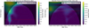 |
Fig. 1. Wavelet spectra of the complete γ-ray LCs of PMN J0531−4827 (left) and PKS 1502+106 (right). The color map represents the signal’s power spectrum, with color intensity indicating the strength of QPO components at different timescales. Yellow represents a higher power, suggesting stronger QPO signals, while purple corresponds to weaker or insignificant variations. This visualization identifies patterns and scales of variability and highlights any QPO presence. The shaded area marks regions where potential modulations are too close to either the sampling interval or the signal’s total duration, reducing reliability, known as the cone of influence (COI). The red horizontal line indicates evidence of transient QPOs. For PMN J0531−4827, a potential transient QPO appears around MJD 55500, with a similar occurrence noted for PKS 1502+106. |
PKS 1502+106 was proposed as a neutrino candidate by Britzen et al. (2021), who identified a periodicity of approximately 3 years in γ-ray emission within a time frame similar to our observations. However, their study did not include a statistical significance analysis, highlighting the need for future investigation. They considered the possibility of a binary SMBHsystem as the driving mechanism behind the observables.
The Fermi-LAT data analysis was performed following the procedure detailed in Peñil et al. (2022), Rico et al. (2025). In particular, we used a binned likelihood analysis considering all data ≥0.1 GeV. The data were binned in 28-day time bins, allowing us to study the long-term behavior of the emission of the selected sources. Their LCs are shown in Figs. 2 and A.1.
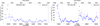 |
Fig. 2. LCs where the CWT analysis indicates the presence of a potential transient QPO. Left: Segment of the LC of PMN J0531−4827 with a potential presence of QPO. Right: γ-ray LC of PKS 1502+106. These LCs are further analyzed in detail in Sect. 5, where we investigate the temporal behavior; we present our theoretical modeling in Sect. 4. |
3. Methodology
This section details the methodology employed to analyze the LCs and identify their key properties, providing the foundation for the flux analysis of each blazar.
3.1. Methods used in the search for QPOs
After the first screening performed during the source sample selection (see Sect. 2), we based the QPO evaluation on two different techniques, the singular spectrum analysis (SSA; Greco et al. 2016; Nina Golyandina 2020) and the generalized Lomb-Scargle periodogram (GLSP; Zechmeister & Kürster 2009). Singular spectrum analysis is a nonparametric approach that breaks down a time series into its main components since it is able to identify trends, oscillatory patterns, and noise (see Fig. 3). This method is particularly effective for identifying quasiperiodic signals embedded within noisy datasets (Rico et al. 2025). Unlike many other techniques, SSA does not rely on predefined assumptions about periodicity and does not require the signal to be sinusoidal, making it a versatile and reliable tool for detecting QPOs with diverse frequencies andamplitudes.
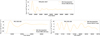 |
Fig. 3. SSA decomposition of LCs of the blazars PMN J0531−4827 (top) and PKS 1502+106 (bottom), revealing the oscillatory component in the signal. The bottom panels show the decomposition of the two analyzed segments of the LC. The oscillatory patterns extracted from the LCs highlight a periodic component, with the inferred periods and uncertainties. The SSA decomposition follows the steps detailed in Rico et al. (2025). |
The second method, GLSP, built on the traditional Lomb-Scargle periodogram (Lomb 1976; Scargle 1982), is a commonly applied tool in periodicity studies dealing with unevenly-sampled, red-noise dominated datasets. The GLSP enhances the original method by accommodating non-sinusoidal periodic signals and integrating weights based on the uncertainties of individual data points, improving its sensitivity and accuracy. This method is applied as a second step after the SSA on the isolated oscillatory component, when any, determining its period and statistical significance over the dominant red noise, following the methodology outlined by Rico et al. (2025). To obtain an approximate estimate of the uncertainty in the derived periods from GLSP and SSA, we adopted the half width at half maximum of the corresponding peaks (e.g., Otero-Santos et al. 2023).
3.2. Test statistics of the QPOs
Identifying QPOs in time-series data is often complicated by noise, which can obscure or hinder genuine periodic signals. In blazar LCs, the dominant red noise contribution frequently leads to false detections (Vaughan et al. 2016), as it often mimics the expected behavior of a genuine periodic signal during a few cycles. This, combined with the Poisson white-noise-like component arising from the random photon detection process that particularly affects γ-ray LCs, is the main factor affecting the detectability of real (quasi)periodic signals in AGN time series.
To assess the statistical significance of the QPOs discussed in this work, we adopted the procedure described in Peñil et al. (2022). Following the methodology from Emmanoulopoulos et al. (2013), we generated 150 000 synthetic stochastic LCs that reproduce both the power spectral density and the probability distribution function of the observed data (see the example shown in Fig. 4). These simulations provide a large ensemble of surrogate LCs that serve as a noise-only baseline, allowing us to evaluate how often the peaks in the observed QPOs could arise purely from stochastic variability. The resulting distributions from these synthetic datasets were then used to estimate the confidence levels (quoted as σ values in the next section) associated with the observed QPOs.
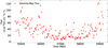 |
Fig. 4. Example of a synthetic LC used to estimate the significance associated with the periods obtained from SSA and GLSP analyses. |
The power spectral density is modeled as a power-law function, A * f−β + C, where A is the normalization, β is the spectral index, f is the frequency, and C accounts for the Poisson noise component. The best fit is obtained through a Maximum Likelihood Estimation method and refined through Markov chain Monte Carlo analysis1. This approach allows for a robustcharacterization of the noise properties of our data, improving the reliability of QPO detections.
3.3. Results
The results derived for the potential QPOs of the two sources analyzed here with the methodology described above are summarized in Table 1. For PMN J0531−4827, the observed QPO period is 188 ± 39 days (2.7σ) using SSA and 213 ± 46 days (1.1σ) with GLSP, showing consistent results within uncertainties. It is important to highlight that the results of the two methods are notably different in terms of the derived significance, suggesting that SSA effectively reduces the contribution of noise components by isolating the genuine QPO, enhancing its detectability with respect to the GLSP.
For PKS 1502+106, the estimated period is 689 ± 108 days (2.4σ) for SSA and 661 ± 72 days (2.1σ) for GLSP. Again, both methods show a very close agreement with the reported values, in this case with a comparable significance level, suggesting a robust periodicity detection. The similarity in results from the two methods indicates that the periodic signal is likely intrinsic rather than an artifact of the analysis technique. However, the moderate significance levels imply that the periodicity is still influenced by the decay in the amplitudes, as visible in Fig. 2, or the reduced number of oscillations of the QPOs.
4. Theoretical model
Several scenarios and hypotheses have been proposed in recent years to interpret QPOs in the emission of AGNs and blazars. One of them, which we adopted in this work, is based on plasma blobs following helical paths within a curved jet (e.g., Sarkar et al. 2021; Prince et al. 2023). In this scenario, the blobs are ejected from the central region, often as a result of instabilities in the accretion disk or magnetic reconnection events near the SMBH (Mohan & Mangalam 2015). These blobs travel outward along the curved jet, maintaining a helical trajectory due to the combined effects of the geometry of the jet and the magnetic field structure. Their motion can then produce quasiperiodic enhancements of the emission whenever they traverse regions of the jet that align with the observer’s line of sight and the opposite effect when the alignment is lower (Fig. 5). In these instances, relativistic beaming modifies the observed intensity. However, as the blob moves within the curved jet, the oscillatory signal diminishes over time, ultimately fading (e.g., Sarkar et al. 2021; Prince et al. 2023).
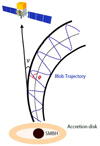 |
Fig. 5. Sketch of the curved jet model based on Sarkar et al. (2021). The angle ϕ represents the inclination between the jet axis and the direction of the plasma blob’s motion, while ψ denotes the angle between the jet axis and the observer’s line of sight. The dotted blue line traces the theoretical trajectory of the plasma blob within the jet, depicting its motion as influenced by the jet’s curvature. |
Several interpretations have been proposed for the origin of this scenario. Rieger (2004) explored how differential Doppler boosting, caused by the helical motion of emitting components within the jet, can lead to observable periodicity. This motion is non-ballistic, meaning the radiating plasma elements follow curved trajectories rather than moving in straight lines. Rieger (2004) identified three possible physical mechanisms for helical jet motion in blazars. The first is non-ballistic motion driven by the orbital motion in an SMBH binary, and thus, the QPO is linked to the orbiting motion of the binary. The second involves either ballistic or non-ballistic helical jet paths induced by jet precession, which may result from gravitational torques exerted by a secondary black hole or from accretion disk warping. The third mechanism attributes non-ballistic helical motion to intrinsic jet instabilities. The first two scenarios are particularly viable for explaining Pobs ≳ 1 year.
Alternatively, distortions in the jet structure could result from the Lense-Thirring effect, where frame-dragging caused by a rotating SMBH induces precession in a tilted accretion disk. This precession propagates down the jet, potentially causing it to bend (e.g., Caproni et al. 2004). A warped accretion disk, driven by gravitational torques or differential radiation pressure, can also induce global precession down to the structure (e.g., Liska et al. 2021).
In another scenario, magnetic fields interacting with the plasma in the accretion disk exert torques that can align ormisalign sections of the disk, depending on the system’s initial configuration (e.g., McKinney et al. 2013). When the disk is misaligned with the SMBH’s spin axis, magnetic torques align the inner disk with the black hole’s equatorial plane, while the misaligned outer disk experiences differential torques. This leads to the precession of the disk plane, which propagates outward and causes changes in the jet’s orientation.
The bending of the jet can also be attributed to the magnetic pressure exerted by an oblique field, which acts asymmetrically on the jet and causes it to deviate from its initial trajectory (Koide 1997). Alternatively, velocity shear between the jet and the surrounding medium can induce Kelvin-Helmholtz instabilities, leading to the formation of helical distortions and potential jet bending (Hardee 1987). Finally, compact objects such as stars, stellar remnants, or dense molecular clouds passing near or through an AGN jet can significantly affect its properties. Their strong gravitational influence may deflect the jet, cause fragmentation, or alter its collimation (e.g., Torres-Albà 2019). In this context, Raiteri et al. (2024) proposed a jet model incorporating an inhomogeneous, curved, and twisting structure, where a wiggling, filamentary jet, interpreted as a rotating double-helix, reproduces the multiwavelength variability of BL Lacs.
4.1. Model expressions
Due to the close alignment of the jet and the line of sight, the emission of blazars is highly enhanced through relativistic Doppler boosting. The relativistic Doppler factor (δ), which quantifies this enhancement, can be expressed as
![Mathematical equation: $$ \begin{aligned} \delta =\frac{1}{\Gamma [1-\beta \cos (\theta )]}, \end{aligned} $$](/articles/aa/full_html/2025/08/aa55599-25/aa55599-25-eq1.gif) (1)
(1)
where Γ is the Lorentz factor, β corresponds to the velocity of the jet in units of the light speed, and θ represents the viewing angle. As introduced above, the helical motion of the blobs along the jet results in changes in the viewing angle. According to Eq. (1), this results in variations in the radiation boosting and, therefore, the observed flux. The helical nature of this trajectory gives place to recurrent changes of the viewing angle θobs(t), inducing the observed quasiperiodic behaviors. This, combined with the curved morphology of the jet, can lead to the transient, fading QPOs observed in these sources. Under this scenario, we can express the viewing angle θobs(t) as a function of the angle between the jet and the direction of the plasma blob – known as pitch angle ϕ – and the angle between the jet and the line of sight ψ, as (see, e.g., Sarkar et al. 2021)
 (2)
(2)
Moreover, we can express the emitted flux as
 (3)
(3)
The Fν and Fν′′ correspond to the observed and rest-frame flux, respectively, n represents the Doppler boosting factor and α is intrinsic spectral index. Taking Eqs. (1) and (2) into account, we can express the sources’ flux as
![Mathematical equation: $$ \begin{aligned} F_{\nu }&\propto \frac{F_{\nu \prime }\prime }{\Gamma ^{(n+\alpha )} (1 + \sin (\phi ) \sin (\psi ))^{(n+\alpha )}} \nonumber \\&\quad \times \left[ 1 - \frac{\beta \cos (\phi ) \cos (\psi )}{1 + \sin (\phi ) \sin (\psi )} \cos \left(\frac{2\pi t}{P_{\rm obs}}\right) \right]^{-(n+\alpha )}. \end{aligned} $$](/articles/aa/full_html/2025/08/aa55599-25/aa55599-25-eq4.gif) (4)
(4)
This emission model is therefore characterized first by the helical motion of the blob along the jet causing the observed recurrent variations and second by the change of the viewing angle of the jet with time, ψ ≡ ψ(t), which describes the fading nature of this quasiperiodic variability. The combination of these two effects describes the time-dependent trajectory of the blob. As a result, flux variations, as expressed in Eq. (4), are directly influenced by the evolving dynamics of ψ(t) and ϕ, providing a framework for interpreting the observed flux variations over time.
4.2. Flux fit
The curved jet model relies on the characteristic exponential decay of oscillations over time as a result of the changing viewing angle as the blob propagates along the jet due to its curved nature. As noted in studies such as Sarkar et al. (2021) and Prince et al. (2023), in this scenario, QPOs often begin with a flaring state, from which the oscillations exhibit initially high amplitudes that progressively decrease in an exponential manner. This behavior is consistent with the transient nature of QPOs and is visually represented in Fig. 2, where the oscillatory amplitudes attenuate over time, consistent with the predictions of the curved jet framework (Sarkar et al. 2021; Prince et al. 2023).
To evaluate this hypothesis, we expressed a temporal variation of ψ as ψ(t)=ae−bt following previous studies based on curved jet scenarios (Sarkar et al. 2021; Prince et al. 2023). This change of the jet viewing angle, coupled with the assumed nature of the motion of the blob, captures the changing amplitude of the QPOs, allowing us to model the observed flux data. Additionally, the model is also dependent on the values of the period of the QPO – derived from our periodicity analysis – the Lorentz factor (Γ), the intrinsic spectral index (α), and the Doppler boosting factor (n).
To assess the quality of the adopted LC model, we employed the R-squared (R2) metric as a measurement of the goodness of the fit. R2 can take values between 0 and 1 (or 0–100 percent). A higher value is indicative of a better agreement between the model and the real data. We adopted the same criteria as in Hair et al. (2011), where three categories or agreement levels are defined based on the value of R2: “weak” for 25%, “moderate” for 50%, and “substantial” for 75%. These thresholds provide a framework for interpreting the accuracy and effectiveness of the model.
5. Results and discussion
We tested for the two selected sources, the curved jet scenario introduced above, where the helical motion of plasma blobs generates periodic variations in the observed flux, while the changing viewing angle of the jet due to its curvature leads to the exponential decay in the QPO amplitudes. As mentioned in Sect. 4.2, this model also depends on other parameters, in particular Γ, β, and ϕ.
No specific Lorentz factors in γ rays were found for these objects in the literature. Consequently, for the Lorentz factors of PKS 1502+106 and PMN J0531−4827, we assumed a value Γ = 15 in our model, within typical values often measured for blazars, as reported by Ghisellini et al. (2010). This can be used to estimate the value of β as Γ = 1/(1 − β−2)1/2, resulting in β = 0.99777. The pitch angle, ϕ, is another variable that is associated with a broad range, typically between 1.5° and 10.0° (e.g., Jorstad et al. 2017; Butuzova 2018). However, no specific pitch angles were obtained from the literature for these blazars; thus, in alignment with Sarkar et al. (2021), Prince et al. (2023), we used a pitch angle of ϕ = 2°.
Moreover, the values of the period Pobs, the index of the exponential function b, the spectral index α, and the Doppler boosting index n are left free to optimize the agreement between the model and the data in the fitting process. We modeled the flux LC for each object with Eq. (4), converging to the values of Pobs, b, α and n that result in the highest value of R2. This process is performed systematically with an iterative approach. We considered values of Pobs within the uncertainty of the period reported in Sect. 3. As for the spectral index, we refer to the mean photon index measured by Singal et al. (2014) in a systematic study of Fermi-LAT blazars, corresponding to a spectral index ∼1.4. Therefore, we tested α values of 1.2, 1.3, 1.4, 1.5, and 1.6 for the model adopted here.
For n, we considered a range of values based on the types of blazars analyzed in this study. As discussed in Sect. 2, our sample includes an FSRQ and a BL Lac, which exhibit different ranges of values of the beaming factor (n) due to variations in their dominant γ-ray emission mechanisms. BL Lacs, characterized by weaker external photon fields compared to FSRQs, predominantly emit through synchrotron radiation and synchrotron self-Compton (SSC) processes (e.g., Ghisellini & Tavecchio 2009). Synchrotron radiation, being more isotropic in the jet’s rest frame, exhibits a relatively weak dependence on the Doppler factor. SSC processes introduce a slightly stronger sensitivity to Doppler boosting but are still moderate compared to the external Compton (EC) mechanisms that dominate in FSRQs. Consequently, for BL Lac objects, the Doppler boosting factor is typically n ≈ 2 − 3 (Dermer 1995). FSRQs are characterized by strong external photon fields originating from the broad-line region, accretion disk, and the dusty torus, which typically make EC scattering the dominant emission mechanism at γ-ray energies (e.g., Ghisellini & Tavecchio 2009). This leads to a higher sensitivity of the observed flux to the Doppler factor, with n ≈ 3 − 5 (Dermer 1995). This heightened sensitivity arises because EC scattering, where seed photons from external sources, such as the accretion disk, broad-line region, or dusty torus, are up-scattered by relativistic electrons, enhances energy transformations more significantly than SSC. The external photon field, which typically has a higher energy density than the synchrotron photon field inside the jet, results in stronger Doppler boosting. As a result, the observed flux becomes more sensitive to the Doppler factor, amplifying the effects of relativistic beaming (Dermer 1995).
Finally, the parameters a and b describing the exponential change of ψ are defined by the pair of values that maximize the goodness of the fit R2, using the initial exponential indices shown in Fig. 6. The results of the optimization of the model for each blazar are summarized in Table 1, and the resulting LC models are shown in Figs. 7 and 9.
 |
Fig. 6. SSA LC decomposition of the studied blazars, revealing the exponential decay component in the signal. Top: PMN J0531−4827. Bottom left: First segment of PKS 1502+106. Bottom right: Second segment of PKS 1502+106. The initial value of the exponential index is indicated for each blazar. The SSA decomposing follows the steps detailed in Rico et al. (2025). |
 |
Fig. 7. LC from Fig. 2, illustrating the flux fit of PMN J0531−4827. Red lines indicate the emission fit based on Eq. (4). The plot legends display the fit parameters, showing the derived period and exponential decay estimated to optimize the R2 value. |
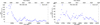 |
Fig. 8. Segments of the LC of PKS 1502+106 analyzed. Left: First segment (54696–56936 MJD). Right: Second segment (56992–58756 MJD). |
5.1. PMN J0531−4827
The fit values are shown in Table 1 and Fig. 7. We obtain an R2 of 46.9%, indicating approximately a “moderate” fit based on the classification described in Sect. 3. The derived values for n and α are 3 and 1.2, respectively. The difference in R2 for n = 2 is 30% smaller. Regarding the values for α, the differences range from 2% to 8%. Figure 10 illustrates the temporal evolution of the jet’s viewing angle, providing key insights into the dynamical changes in its orientation. The inferred period is 191 days. According to the scenarios presented in (see our Sect. 4 Rieger 2004), this result suggests that the underlying physical mechanism is an intrinsic phenomenon within the jet. These can be associated with helical jet instabilities, plasma turbulence, or internal shock interactions. The helical motion of the jet due to magnetohydrodynamic instabilities can lead to periodic variations in emission (Rieger 2004). At the same time, turbulence in the relativistic plasma can introduce quasi-regular fluctuations in the jet structure (Marscher 2014). Additionally, internal shocks caused by variations in the jet’s velocity could create periodic enhancements in particle acceleration, modulating the observed emission and contributing to the QPO (Spada et al. 2001).
5.2. PKS 1502+106
As shown in Fig. 2, we identify two distinct segments in the LC that exhibit potentially transient QPOs. The first segment spans MJD 54696–56936, while the second covers MJD 56992–58756 (Fig. 8). The corresponding oscillatory components extracted via SSA are presented in Fig. 3. Each segment is analyzed independently to evaluate its periodic behavior and underlying physical properties.
5.2.1. First segment
The values of the best fit for the first segment of this source are also reported in Table 1. Moreover, the derived LC model is shown in Fig. 9. In this case, the best fit is found with a goodness value R2 = 55.9%, which can again be considered approximately as a “moderate” fit according to the categorization defined in Sect. 3. The Doppler boosting factor and spectral index converge to values of n = 3 and α = 1.2 as for the previous case, with a degradation of R2 down to 37% for larger values of n and 20% in the case of α. Figure 10 depicts the temporalevolution of the jet’s viewing angle, changing from ∼0.2° to ∼1.4°, highlighting its characteristic exponential decay over time.
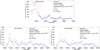 |
Fig. 9. Flux fits of each analyzed segment of PKS 1502+106. Top: First segment (54696–56936 MJD). Bottom: Second segment (54992–58756). For this segment, two different flux fits are done, based on the two potential periods reported for the QPO. Left: Flux fit considering a period of 283 ± 47. Right: Flux fit considering a period of 593 ± 53. Red lines indicate the emission fit based on Eq. (4). The plot legends display the fit parameters, showing the derived period and exponential decay estimated to optimize the R2 value. |
5.2.2. Second segment
The second segment of the LC of PKS 1502+106 yields two different candidate periods based on the analysis using SSA and the GLSP. As shown in Table 1, both detected periods have a relatively low significance (≤1.5). The first period, reported by SSA, is 283 ± 47 days, while the second, at 593 ± 63 days, is consistent with the period found in the first segment of the LC (see Fig. A.2).
To explore the potential periodic modulation of the flux, we performed two separate exponential fits using each of the candidate periods. The fit associated with the ≈300-day period yields an R2 value of 42.7%, while the fit using the ≈600-day period gives a lower R2 of 32.4%. The parameters a and b from the exponential model are compatible in both cases, suggesting a similar flux evolution trend regardless of the assumed period. However, based on the higher R2 value, the fit associated with the ≈300-day period is favored. This suggests that the ≈300-day period provides a better description of the observed flux modulation in the second segment of the LC. Figure 10 shows the temporal evolution of the jet’s viewing angle, from ∼0.8° to ∼1.3° degrees, significantly different from the viewing angle evolution of the first segment.
 |
Fig. 10. Jet viewing angle (ψ) as a function of time. Top: PMN J0531−4827. Center: PKS 1502+106, first segment. Bottom: PKS 1502+106, second segment. We use the parameters with best R2 (Table 1). The panels for PKS 1502+106 show the differences in the jet viewing angle that are the consequence of the different exponential trend fits (Table 1). |
5.2.3. Discussion
The inferred period of ≈600 days in the first segment of the LC can be attributed to the helical motion of a plasma blob along the jet, a scenario commonly associated with binary SMBH systems. As suggested by Rieger (2004), such long-term periodicities could arise from the orbital motion in a binary SMBH system (see Sect. 4). Indeed, the possibility of a binary SMBH at the core of PKS 1502+106 has previously been proposed by Britzen et al. (2021). In this context, Villata & Raiteri (1999) predicted that the relativistic jet could become bent due to the orbital dynamics of the binary system. Additionally, Raiteri et al. (2017) show that interactions between the magnetized jet plasma and the surrounding environment can induce a helical twist in the jet structure. This type of geometry may contribute to periodic variability in the observed flux via relativistic Doppler modulation, as also discussed by Liska et al. (2021) in the context of precessing accretion flows.
The second segment of the LC yields two possible periods with relatively low significance, complicating the interpretation. One of these periods (≈600 days) is consistent with the period found in the first segment, providing additional, though tentative, support for the binary SMBH scenario. However, the alternative period of approximately ≈300 days results in a better fit to the flux modulation, as indicated by the higher R2. Although Rieger (2004) also considered binary systems capable of producing shorter periodicities (1-year-like QPOs), the lack of consistency between the two candidate periods casts doubt on the binary scenario as a unique explanation.
Additionally, the exponential flux trend parameters (specifically, the a and b coefficients) differ between the two segments. This discrepancy suggests a variation in the Doppler boosting factor, which can be interpreted as a change in the jet’s viewing angle, as shown in Fig. 10.
Despite the inconsistencies found after analyzing the two transient QPOs, the binary scenario cannot be discarded completely. The binary interaction could result in complex scenarios, resulting in a complex structure in the LC (e.g., Qian et al. 2019; Britzen et al. 2018). For instance, in the case of PKS 1502+106, during a different orbital phase, the geometry of the system may cause the jet to sweep past the observer’s line of sight much more rapidly. This could occur if the orbital motion causes a sharper angular curvature in the jet trajectory. In this scenario, the alignment with the observer is brief and less stable. Therefore, the Doppler factor peaks quickly and then declines rapidly as the angle shifts away. The resulting QPO event would appear sharper, with a steeper exponential decay in the LC following the maximum (first transient QPO). In contrast, during another orbital phase, the jet axis may shift more gradually into near-perfect alignment with the observer’s line of sight. In this case, these conditions are sustained for leading to a smoother decay in the QPO amplitude after the peak, exhibiting a slow exponential decay in flux (second transient QPO). However, during these phases, other intrinsic jet processes (Marscher 2014) may become more prominent in the observed LCs. Such phenomena, like turbulence or localized particle acceleration, can overlap with or obscure the primary QPO signature, complicating the identification of a consistent period for the two transient QPOs. Britzen et al. (2021) proposed the presence of a curved jet in PKS 1502+106, whose kinematics appear perturbed by the surrounding, such as narrow-line region clouds or disk-driven winds, further increasing the complexity of the jet.
Therefore, the results for PKS 1502+106 could suggest that a single, curved jet structure is not fully accounted for the transient nature of the QPOs observed in this blazar. The variability in the both period and flux profile points to a more complex scenario, possibly involving multiple physical mechanisms (Britzen et al. 2021), not necessarily considering the binary system. In this context, a possible explanation for the QPOs of this blazar is provided by the interaction between a plasma blob and standing shocks within relativistic jets. As shown by Fichet de Clairfontaine et al. (2022), when a high-speed perturbation encounters a recollimation shock, it can trigger a sequence of relaxation shocks that propagate downstream. These relaxation shocks act as secondary dissipation sites, producing delayed emission events or “flare echoes”. Due to the progressive energy dissipation and the weakening of the shock structure over time, each subsequent emission episode can appear fainter, potentially leading to an exponentially decaying profile.
An alternative explanation is provided by the model proposed by Wiita (2011). In this framework, non-axisymmetric magnetic field structures within the jet create localized irregularities. As a shock wave propagates outward, it interacts with these inhomogeneities, producing fluctuations in the emitted flux. When the shock moves through a helical structure within the jet, the effect is similar to a change in the jet’s direction, resulting in an apparent shift in the viewing angle. If the jet remains approximately cylindrical and the shock velocity is constant, the emission pattern can maintain a consistent period, especially if similar helical structures are encountered sequentially. Furthermore, Wiita (2011) suggests that turbulence behind a propagating shock can also generate quasiperiodic features. In this scenario, a dominant turbulent cell can periodically enhance the emission via Doppler boosting. However, due to the stochastic and decaying nature of turbulence, the amplitude of such QPOs will diminish over time. Changes in the size, strength, or speed of the turbulent cells can also cause variations in the observed period.
6. Summary
We have investigated the transient QPOs observed in the γ-ray emission of blazars PMN J0531−4827 and PKS 1502+106 using over a decade of Fermi-LAT observations. Through the analysis of their LCs, we characterized the periods of these transient QPOs, with values of ≈200 days for PMN J0531−4827. In the case of PKS 1502+106, we analyzed two independent segments exhibiting QPO-like behavior, both of which suggested a characteristic period of ≈600 days. However, in the second segment, an alternative solution with a period of ≈300 days provided a better fit to the flux modulation pattern. Concerning the physical origin of these transient QPOs, the oscillation detected in PMN J0531−4827 can plausibly be interpreted within the framework of a curved jet scenario.
For PKS 1502+106, we initially explored a curved jet scenario in which the observed quasiperiodic behavior could result from jet precession, potentially induced by a binary SMBH system. However, modeling the two QPO segments requires a discontinuous shift in phase around MJD 57000, from ψ = 1.4° to ψ = 0.8°, which is difficult to reconcile with the smooth, continuous precession expected in binary-driven scenarios. Moreover, the differing temporal evolution and decay patterns across the two segments are inconsistent with the stable, long-term periodic modulation typically associated with binary-induced jet wobble. These aspects break the continuity of the curved jet model and challenge its physical plausibility in this context. As a more plausible alternative, we propose that the QPOs in PKS 1502+106 arise from internal shocks within the relativistic jet. This interpretation is consistent with recent models of relaxation shocks in perturbed jets and naturally explains the transient, evolving character of the observed QPOs.
We utilized the PYTHON package emcee.
Acknowledgments
P.P. and M.A. acknowledge funding under NASA contract 80NSSC20K1562. J.O.-S. acknowledges founding from the Istituto Nazionale di Fisica Nucleare (INFN) Cap. U.1.01.01.01.009. This work was supported by the European Research Council, ERC Starting grant MessMapp, S.B. Principal Investigator, under contract no. 949555, and by the German Science Foundation DFG, research grant “Relativistic Jets in Active Galaxies” (FOR 5195, grant No. 443220636).
References
- Adhikari, S., Peñil, P., Westernacher-Schneider, J. R., et al. 2024, ApJ, 965, 124 [CrossRef] [Google Scholar]
- Akiyama, M., Ueda, Y., Ohta, K., Takahashi, T., & Yamada, T. 2003, ApJS, 148, 275 [NASA ADS] [CrossRef] [Google Scholar]
- Atwood, W. B., Abdo, A. A., Ackermann, M., et al. 2009, ApJ, 697, 1071 [CrossRef] [Google Scholar]
- Ballet, J., Burnett, T. H., Digel, S. W., & Lott, B. 2020, ArXiv e-prints [arXiv:2005.11208] [Google Scholar]
- Britzen, S., Fendt, C., Witzel, G., et al. 2018, MNRAS, 478, 3199 [NASA ADS] [Google Scholar]
- Britzen, S., Zajaček, M., Popović, L. Č., et al. 2021, MNRAS, 503, 3145 [NASA ADS] [CrossRef] [Google Scholar]
- Butuzova, M. S. 2018, Astron. Rep., 62, 116 [Google Scholar]
- Camenzind, M., & Krockenberger, M. 1992, A&A, 255, 59 [NASA ADS] [Google Scholar]
- Caproni, A., Mosquera Cuesta, H. J., & Abraham, Z. 2004, ApJ, 616, L99 [Google Scholar]
- Caproni, A., Abraham, Z., Motter, J. C., & Monteiro, H. 2017, ApJ, 851, L39 [NASA ADS] [CrossRef] [Google Scholar]
- Chen, J., Yu, J., Huang, W., & Ding, N. 2024, MNRAS, 528, 6807 [NASA ADS] [CrossRef] [Google Scholar]
- Covino, S., Sandrinelli, A., & Treves, A. 2018, MNRAS, 482, 1270 [Google Scholar]
- Dermer, C. D. 1995, ApJ, 446, L63 [NASA ADS] [CrossRef] [Google Scholar]
- Emmanoulopoulos, D., McHardy, I. M., & Papadakis, I. E. 2013, MNRAS, 433, 907 [NASA ADS] [CrossRef] [Google Scholar]
- Fan, J.-H. 2005, Chin. J. Astron. Astrophys. Suppl., 5, 213 [NASA ADS] [CrossRef] [Google Scholar]
- Fichet de Clairfontaine, G., Meliani, Z., & Zech, A. 2022, A&A, 661, A54 [NASA ADS] [CrossRef] [EDP Sciences] [Google Scholar]
- Fragile, P. C., & Meier, D. L. 2009, ApJ, 693, 771 [CrossRef] [Google Scholar]
- Franchini, A., Lodato, G., & Facchini, S. 2016, MNRAS, 455, 1946 [NASA ADS] [CrossRef] [Google Scholar]
- Ghisellini, G., & Tavecchio, F. 2009, MNRAS, 397, 985 [Google Scholar]
- Ghisellini, G., Celotti, A., Fossati, G., Maraschi, L., & Comastri, A. 1998, MNRAS, 301, 451 [NASA ADS] [CrossRef] [Google Scholar]
- Ghisellini, G., Tavecchio, F., Foschini, L., et al. 2010, MNRAS, 402, 497 [Google Scholar]
- Gong, Y., Tian, S., Zhou, L., Yi, T., & Fang, J. 2023, ApJ, 949, 39 [Google Scholar]
- Greco, G., Kondrashov, D., Kobayashi, S., et al. 2016, in The Universe of Digital Sky Surveys, eds. N. R. Napolitano, G. Longo, M. Marconi, M. Paolillo,&E. Iodice, Astrophys. Space Sci. Proc., 42, 105 [Google Scholar]
- Hair, J., Ringle, C., & Sarstedt, M. 2011, J. Mark. Theory Pract., 19, 139 [CrossRef] [Google Scholar]
- Hardee, P. E. 1987, ApJ, 318, 78 [Google Scholar]
- Jorstad, S. G., Marscher, A. P., Morozova, D. A., et al. 2017, ApJ, 846, 98 [Google Scholar]
- Koide, S. 1997, ApJ, 478, 66 [Google Scholar]
- Liska, M., Hesp, C., Tchekhovskoy, A., et al. 2021, MNRAS, 507, 983 [NASA ADS] [CrossRef] [Google Scholar]
- Lister, M. L. 2001, ApJ, 562, 208 [NASA ADS] [CrossRef] [Google Scholar]
- Lomb, N. R. 1976, Ap&SS, 39, 447 [Google Scholar]
- Marscher, A. P. 2014, ApJ, 780, 87 [Google Scholar]
- Marscher, A. P., Gear, W. K., & Travis, J. P. 1992, in Variability of Blazars, eds. E. Valtaoja,&M. Valtonen, 85 [Google Scholar]
- McKinney, J. C., Tchekhovskoy, A., & Blandford, R. D. 2013, Science, 339, 49 [NASA ADS] [CrossRef] [Google Scholar]
- Mohan, P., & Mangalam, A. 2015, ApJ, 805, 91 [CrossRef] [Google Scholar]
- Nina Golyandina, A. Z. 2020, Singular Spectrum Analysis for Time Series, 2nd edn. (Berlin, Heidelberg: Springer) [Google Scholar]
- Otero-Santos, J., Peñil, P., Acosta-Pulido, J. A., et al. 2023, MNRAS, 518, 5788 [Google Scholar]
- Peñil, P., Domínguez, A., Buson, S., et al. 2020, ApJ, 896, 134 [CrossRef] [Google Scholar]
- Peñil, P., Ajello, M., Buson, S., et al. 2022, ArXiv e-prints [arXiv:2211.01894] [Google Scholar]
- Peñil, P., Otero-Santos, J., Ajello, M., et al. 2024, MNRAS, 529, 1365 [Google Scholar]
- Peñil, P., Domínguez, A., Buson, S., et al. 2025, ApJ, 980, 38 [Google Scholar]
- Prince, R., Banerjee, A., Sharma, A., et al. 2023, A&A, 678, A100 [NASA ADS] [CrossRef] [EDP Sciences] [Google Scholar]
- Qian, S. J. 2022, ArXiv e-prints [arXiv:2206.14995] [Google Scholar]
- Qian, S. J., Britzen, S., Krichbaum, T. P., & Witzel, A. 2019, A&A, 621, A11 [NASA ADS] [CrossRef] [EDP Sciences] [Google Scholar]
- Raiteri, C. M., Villata, M., Acosta-Pulido, J. A., et al. 2017, Nature, 552, 374 [NASA ADS] [CrossRef] [Google Scholar]
- Raiteri, C. M., Villata, M., Carnerero, M. I., et al. 2024, A&A, 692, A48 [NASA ADS] [CrossRef] [EDP Sciences] [Google Scholar]
- Rico, A., Domínguez, A., Peñil, P., et al. 2025, A&A, 697, A35 [NASA ADS] [CrossRef] [EDP Sciences] [Google Scholar]
- Rieger, F. M. 2004, ApJ, 615, L5 [NASA ADS] [CrossRef] [Google Scholar]
- Roy, A., Chitnis, V. R., Gupta, A. C., et al. 2022, MNRAS, 513, 5238 [Google Scholar]
- Ruan, J. J., Anderson, S. F., MacLeod, C. L., et al. 2012, ApJ, 760, 51 [Google Scholar]
- Sandrinelli, A., Covino, S., Dotti, M., & Treves, A. 2016, AJ, 151, 54 [NASA ADS] [CrossRef] [Google Scholar]
- Sarkar, A., Kushwaha, P., Gupta, A. C., Chitnis, V. R., & Wiita, P. J. 2020, A&A, 642, A129 [NASA ADS] [CrossRef] [EDP Sciences] [Google Scholar]
- Sarkar, A., Gupta, A. C., Chitnis, V. R., & Wiita, P. J. 2021, MNRAS, 501, 50 [Google Scholar]
- Scargle, J. D. 1982, ApJ, 263, 835 [Google Scholar]
- Singal, J., Ko, A., & Petrosian, V. 2014, ApJ, 786, 109 [NASA ADS] [CrossRef] [Google Scholar]
- Sobacchi, E., Sormani, M. C., & Stamerra, A. 2017, MNRAS, 465, 161 [NASA ADS] [CrossRef] [Google Scholar]
- Spada, M., Ghisellini, G., Lazzati, D., & Celotti, A. 2001, MNRAS, 325, 1559 [NASA ADS] [CrossRef] [Google Scholar]
- Titov, O., Pursimo, T., Johnston, H. M., et al. 2017, AJ, 153, 157 [Google Scholar]
- Torrence, C., & Compo, G. P. 1998, BAMS, 79, 61 [NASA ADS] [CrossRef] [Google Scholar]
- Torres-Albà, N. 2019, High Energy Phenomena in Relativistic Outflows VII, 5 [Google Scholar]
- Valtonen, M. J., Lehto, H. J., Nilsson, K., et al. 2008, Nature, 452, 851 [Google Scholar]
- Vaughan, S., Uttley, P., Markowitz, A., et al. 2016, MNRAS, 461, 3145 [NASA ADS] [CrossRef] [Google Scholar]
- Villata, M., & Raiteri, C. M. 1999, A&A, 347, 30 [NASA ADS] [Google Scholar]
- Wiita, P. J. 2006, ArXiv e-prints [arXiv:astro-ph/0603728] [Google Scholar]
- Wiita, P. J. 2011, J. Astrophys. Astron., 32, 147 [Google Scholar]
- Zechmeister, M., & Kürster, M. 2009, A&A, 496, 577 [CrossRef] [EDP Sciences] [Google Scholar]
Appendix A: Figures
This section includes the complete γ-ray LCs of PMN J0531−4827 (Fig. A.1). Additionally, we include the complete LC of PKS 1502+106, denoting the potential high-flux emission states based on a period of 600 days, an approximation of the results obtained in Sect. 5.2 (Fig. A.2).
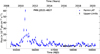 |
Fig. A.1. γ-ray LC of PMN J0531−4827. |
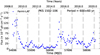 |
Fig. A.2. γ-ray LC of PKS 1502+106. The gray vertical bars are used to approximate the high-flux periods, based on a period of ≈600 days, which are suggested by our analysis. The width of these gray bars represents the uncertainty associated with the periodic signal, which is an approximation of the results included in Table 1. |
All Tables
All Figures
|
Fig. 1. Wavelet spectra of the complete γ-ray LCs of PMN J0531−4827 (left) and PKS 1502+106 (right). The color map represents the signal’s power spectrum, with color intensity indicating the strength of QPO components at different timescales. Yellow represents a higher power, suggesting stronger QPO signals, while purple corresponds to weaker or insignificant variations. This visualization identifies patterns and scales of variability and highlights any QPO presence. The shaded area marks regions where potential modulations are too close to either the sampling interval or the signal’s total duration, reducing reliability, known as the cone of influence (COI). The red horizontal line indicates evidence of transient QPOs. For PMN J0531−4827, a potential transient QPO appears around MJD 55500, with a similar occurrence noted for PKS 1502+106. |
| In the text | |
|
Fig. 2. LCs where the CWT analysis indicates the presence of a potential transient QPO. Left: Segment of the LC of PMN J0531−4827 with a potential presence of QPO. Right: γ-ray LC of PKS 1502+106. These LCs are further analyzed in detail in Sect. 5, where we investigate the temporal behavior; we present our theoretical modeling in Sect. 4. |
| In the text | |
|
Fig. 3. SSA decomposition of LCs of the blazars PMN J0531−4827 (top) and PKS 1502+106 (bottom), revealing the oscillatory component in the signal. The bottom panels show the decomposition of the two analyzed segments of the LC. The oscillatory patterns extracted from the LCs highlight a periodic component, with the inferred periods and uncertainties. The SSA decomposition follows the steps detailed in Rico et al. (2025). |
| In the text | |
|
Fig. 4. Example of a synthetic LC used to estimate the significance associated with the periods obtained from SSA and GLSP analyses. |
| In the text | |
|
Fig. 5. Sketch of the curved jet model based on Sarkar et al. (2021). The angle ϕ represents the inclination between the jet axis and the direction of the plasma blob’s motion, while ψ denotes the angle between the jet axis and the observer’s line of sight. The dotted blue line traces the theoretical trajectory of the plasma blob within the jet, depicting its motion as influenced by the jet’s curvature. |
| In the text | |
|
Fig. 6. SSA LC decomposition of the studied blazars, revealing the exponential decay component in the signal. Top: PMN J0531−4827. Bottom left: First segment of PKS 1502+106. Bottom right: Second segment of PKS 1502+106. The initial value of the exponential index is indicated for each blazar. The SSA decomposing follows the steps detailed in Rico et al. (2025). |
| In the text | |
|
Fig. 7. LC from Fig. 2, illustrating the flux fit of PMN J0531−4827. Red lines indicate the emission fit based on Eq. (4). The plot legends display the fit parameters, showing the derived period and exponential decay estimated to optimize the R2 value. |
| In the text | |
|
Fig. 8. Segments of the LC of PKS 1502+106 analyzed. Left: First segment (54696–56936 MJD). Right: Second segment (56992–58756 MJD). |
| In the text | |
|
Fig. 9. Flux fits of each analyzed segment of PKS 1502+106. Top: First segment (54696–56936 MJD). Bottom: Second segment (54992–58756). For this segment, two different flux fits are done, based on the two potential periods reported for the QPO. Left: Flux fit considering a period of 283 ± 47. Right: Flux fit considering a period of 593 ± 53. Red lines indicate the emission fit based on Eq. (4). The plot legends display the fit parameters, showing the derived period and exponential decay estimated to optimize the R2 value. |
| In the text | |
|
Fig. 10. Jet viewing angle (ψ) as a function of time. Top: PMN J0531−4827. Center: PKS 1502+106, first segment. Bottom: PKS 1502+106, second segment. We use the parameters with best R2 (Table 1). The panels for PKS 1502+106 show the differences in the jet viewing angle that are the consequence of the different exponential trend fits (Table 1). |
| In the text | |
|
Fig. A.1. γ-ray LC of PMN J0531−4827. |
| In the text | |
|
Fig. A.2. γ-ray LC of PKS 1502+106. The gray vertical bars are used to approximate the high-flux periods, based on a period of ≈600 days, which are suggested by our analysis. The width of these gray bars represents the uncertainty associated with the periodic signal, which is an approximation of the results included in Table 1. |
| In the text | |
Current usage metrics show cumulative count of Article Views (full-text article views including HTML views, PDF and ePub downloads, according to the available data) and Abstracts Views on Vision4Press platform.
Data correspond to usage on the plateform after 2015. The current usage metrics is available 48-96 hours after online publication and is updated daily on week days.
Initial download of the metrics may take a while.