| Issue |
A&A
Volume 700, August 2025
|
|
|---|---|---|
| Article Number | A245 | |
| Number of page(s) | 16 | |
| Section | Interstellar and circumstellar matter | |
| DOI | https://doi.org/10.1051/0004-6361/202555901 | |
| Published online | 25 August 2025 | |
CHemical Evolution in MassIve star-forming COres (CHEMICO)
I. Evolution of the temperature structure
1
INAF – Osservatorio Astrofisico di Arcetri,
Largo E. Fermi 5,
50125
Florence,
Italy
2
LUX, Observatoire de Paris, PSL Research University, CNRS, Sorbonne Université,
92190
Meudon,
France
3
Max-Planck-Institut für extraterrestrische Physik,
Giessenbachstraße 1,
85748
Garching bei München,
Germany
4
Centro de Astrobiología (CAB), CSIC-INTA,
Ctra. de Ajalvir Km. 4,
28850
Torrejón de Ardoz, Madrid,
Spain
5
Dipartimento di Chimica “Giacomo Ciamician”, Università di Bologna,
Via P. Gobetti 85,
40129
Bologna,
Italy
6
INAF – Istituto di Astrofisica e Planetologia Spaziali,
Via Fosso del Cavaliere 100,
00133
Roma,
Italy
7
Research Laboratory for Astrochemistry, Ural Federal University,
Kuibysheva St. 48,
Yekaterinburg
620026,
Russia
★ Corresponding author: This email address is being protected from spambots. You need JavaScript enabled to view it.
Received:
11
June
2025
Accepted:
1
July
2025
Abstract
Context. Increasing evidence shows that most stars in the Milky Way, including the Sun, are born in star-forming regions that also contain high-mass stars. However, due to both observational and theoretical challenges, our understanding of their chemical evolution is much less clear than that of their low-mass counterparts.
Aims. In this work, we present the project ‘CHemical Evolution of MassIve star-forming COres’ (CHEMICO). The project aims to investigate aspects of the chemical evolution of high-mass star-forming cores by observing representatives of the three main evolutionary categories: high-mass starless cores, high-mass protostellar objects, and ultra-compact HII (UCHII) regions.
Methods. We carried out an unbiased spectral line survey of the entire bandwidth at 3, 2, and 1.2 mm with the 30m telescope of the Insitut de Radioastronomie millimétrique towards three targets that represent the three evolutionary stages.
Results. The number of detected lines and species increases with evolution. In this first study, we derive the temperature structure of the targets through the analysis of the carbon-bearing species C2H, c-C3H, c-C3H2, C4H, CH3CCH, HC3N, CH3CN, and HC5N. The excitation temperature, Tex, increases with evolution in each species, although not uniformly. Hydrocarbons tend to be associated with the smallest Tex values and enhancements with evolution, while cyanides are associated with the highest Tex values and enhancements. In each target, the higher the number of atoms in the molecule, the higher Tex tends to be.
Conclusions. The temperature structure evolves from a cold (~20 K), uniform envelope traced by simple hydrocarbons in the high-mass starless core stage, to a more stratified envelope in the protostellar stage made by a hot core (≥100 K), an intermediate shell with Tex ~30–60 K, and a larger cold envelope. Finally, in the UCHII stage, a hot core surrounded only by a cold envelope remains. These results suggest a steepening of the Tex radial profile as a function of time.
Key words: astrochemistry / stars: formation / stars: massive / stars: protostars / ISM: clouds / ISM: molecules
© The Authors 2025
 Open Access article, published by EDP Sciences, under the terms of the Creative Commons Attribution License (https://creativecommons.org/licenses/by/4.0), which permits unrestricted use, distribution, and reproduction in any medium, provided the original work is properly cited.
This article is published in open access under the Subscribe to Open model. This email address is being protected from spambots. You need JavaScript enabled to view it. to support open access publication.
1 Introduction
Growing evidence now indicates that our Sun was born in a crowded stellar cluster including high-mass stars, i.e. stars more massive than ~8 M⊙ (e.g. Adams 2010; Pfalzner et al. 2015; Jensen et al. 2019; Arzoumanian et al. 2023). The case of the Sun is not unique, as it is now well established that most stars are born in rich clusters (e.g. Carpenter 2000; Lada & Lada 2003) which likely included high-mass stars (e.g. Rivilla et al. 2014). Therefore, studying the properties of high-mass star-forming regions can provide important information not only on the formation of high-mass stars but also on the heritage of both the Solar System and most stars in the Milky Way.
Our knowledge of how high-mass stars are born is still limited, owing to both observational and theoretical problems (e.g. Zinnecker & Yorke 2007; Tan et al. 2014; Krumholz 2015; Motte et al. 2018). Observations are challenging because (i) there are fewer high-mass star-forming cores (i.e. molecular compact structures) that have the potential to form high-mass stars and/or clusters with respect to their low-mass counterparts, (ii) they have smaller angular dimensions (being located at distances ≥1 kpc), and (iii) they are typically ‘polluted’ by large amounts of ambient gas and/or nearby star formation activity. Theoretical problems arise primarily from the fact that high-mass star-forming cores evolve over timescales of ≤105 years, typically shorter than those of their low-mass counterparts, and, in particular, accretion persists longer than contraction (Yorke 1986). This implies that high-mass stars switch on while still accreting and the radiation pressure of the embryo star could be sufficient to impede any further accretion (Larson & Starrfield 1971; Appenzeller & Tscharnuter 1974). Although models can address this problem (e.g. McKee & Tan 2003; Bonnell et al. 2004), the steps of the high-mass star formation process remain debated and are not clearly separated into evolutionary classes, as is the case for the low-mass star formation process (see, e.g., Shu et al. 1987; André et al. 2000). Therefore, identifying a chemical evolutionary sequence would be extremely useful in defining a physical evolutionary sequence that is still uncertain.
Several attempts have been made to empirically classify pc-scale high-mass star-forming cores in different evolutionary stages (e.g. Tan et al. 2014; Motte et al. 2018). Following the sequence established for low-mass star-forming cores, these schemes typically divide the evolution into three main phases (see Fig. 1). The earliest stage is that of high-mass starless cores (HMSCs). These objects, mostly found in infrared-dark, dense molecular clouds, are in a physical stage immediately before (or at the very beginning of) the gravitational collapse. They are characterised by low kinetic temperatures (Tk~10–20 K) and exhibit high densities (n ≥ 103−105 cm−3, depending on size). They can also show evidence of outflows or signs of star formation at very early stage, or such indications may be entirely absent. During these early cold phases, atoms and simple molecules are thought to freeze out onto dust grain surfaces. As a result, surface chemistry is very active, and gas-phase chemistry processes, particularly neutral-neutral and endothermic reactions, are inhibited. As evolution proceeds, these cores transition into high-mass protostellar objects (HMPOs). These are collapsing cores with evidence of deeply embedded protostar(s), typically characterised by higher densities and temperatures than in the previous stage (n ≃ 106 cm−3, Tk ≥ 20 K). In these warm(er) environments, molecules in the mantles sublimate back into the gas phase, and reactions inefficient at low temperatures proceed and form new complex molecules. Collimated jets and molecular outflows from the protostar(s) can also trigger local high-energy, non-equilibrium chemistry typical of shocked gas. The final phase corresponds to the formation of ultra-compact HII regions (UCHIIIs). These cores contain at least one embedded zero-age main-sequence star associated with an expanding HII region. The surrounding molecular cocoon (n ≥ 105 cm−3, Tk~20–100 K) can be influenced by its progressive expansion and by heating and irradiation from the central star.
Chemical and physical evolution are expected to proceed in parallel, but only an unbiased survey of the whole (sub-)millimetre band towards sources with well-established evolutionary stages can fully characterise the chemical evolution from one stage to another. In particular, identifying evolutionary diagnostic tools for use in future studies of larger samples is crucial. Such studies can also provide constraints on chemicaldynamical models (e.g. Sipilä & Caselli 2018) of high-mass star-forming regions, elucidating important chemical processes occurring at the three different evolutionary stages, which, in turn, will help to link these stages in a unified scenario. Previous studies have highlighted potential evolutionary indicators that are particularly useful for tracing specific phases. For example, certain deuterated molecules are excellent tracers of the earliest stages (e.g. Fontani et al. 2011, 2015a; Sabatini et al. 2024), whereas some complex organic molecules (COMs) or sulphur-bearing species appear to trace later phases (e.g. Coletta et al. 2020; Fontani et al. 2023).
We present the project ‘CHemical Evolution in Massive star-forming COres’ (CHEMICO), in which we perform the first full spectral survey in the millimetre bands with the Institut de RadioAstronomie Millimétrique (IRAM) 30m telescope towards three dense cores that best represent the three evolutionary stages of high-mass star formation. The observed lines allow us to derive the column densities of all the molecules detected from all observable transitions. From the molecular column densities, the abundances are also derived using the H2 column densities, N(H2), previously calculated for all objects (Fontani et al. 2018). Because chemical evolution has been studied extensively for low-mass star-forming cores (see, e.g. the reviews by Caselli & Ceccarelli 2012; Jørgensen et al. 2020), this project also aims to compare chemical evolution in the low- and high-mass regimes.
In this paper, we present the data, sample, and method used to identify and analyse the molecules. We also present the analysis of some carbon-chain and hydrocarbon species. Carbon chains are ubiquitous in the interstellar medium and have been linked to the evolutionary stage in low-mass star-forming regions (see, e.g. Taniguchi et al. 2024 and references therein). The fact that they can be formed from atomic carbon (e.g. Suzuki et al. 1992; Taniguchi et al. 2019) suggests that their production is favoured before CO formation, that is, in the early stages of star formation. This interpretation agrees with the detection of long hydrocarbons and cyanopolyynes in cold, dark cores (Loren et al. 1984; Cernicharo et al. 2021; Loomis et al. 2021). However, this simple scenario is challenged by the fact that carbon-chain and carbon-rich species (which we define in this study as molecules with at least three carbon atoms and no oxygen) are also abundant in warm (T ≥ 30 K) low-mass and high-mass protostellar cores (e.g. Sakai & Yamamoto 2013; Taniguchi et al. 2023). For example, reactions originating from gaseous methane (CH4) evaporated from ice mantles, have been invoked to explain their abundances in the evolved protostellar stages (e.g. Sakai & Yamamoto 2013). Carbon chains also increase their abundances in the presence of locally accelerated cosmic rays (e.g. Fontani et al. 2017), as well as in the cavity walls of outflows (e.g. Zhang et al. 2018; Tychoniec et al. 2021). Furthermore, carbon-chain and other carbon-rich species, such as CH3CCH and HC3N, are commonly used as temperature tracers (e.g. Fontani et al. 2002; Taniguchi et al. 2019) in star-forming cores, owing to their molecular structure and the large number of rotational transitions observable in the (sub-)millimetre regime. Understanding the temperature variations in the targets is critical for properly modelling the chemistry. Therefore, in this first paper we analyse carbon-chain and carbon-rich species not only to inspect how their abundances vary with evolution but also to investigate variations in the thermal structure of the cores. In this context, we also include in our study the analysis of CH3CN, a carbon-bearing COM that is neither a carbon-chain nor a carbon-rich species, but serves as a good gas thermometer and a species sensitive to evolution (e.g. Mininni et al. 2021).
The paper is organised as follows. Sect. 2 presents the source sample. In Sect. 3 we describe the observations and the procedures adopted for data reduction, line identification, and analysis. Section 4 presents the line and the physical parameters derived from the detected carbon-bearing species. In Sect. 5, we discuss our results, with emphasis on the evolution of both the temperature structure(s) and the molecular abundances. Conclusions and future steps of this project are summarised in Sect. 6.
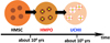 |
Fig. 1 Scheme of the coarse evolutionary classification for high-mass star-forming cores in HMSCs, HMPOs, and UCHIIs (Colzi 2020, adapted from Motte et al. 2018). |
Source coordinates and basic physical parameters.
2 Sample
The sources are part of a sample that has been extensively studied over the past decade, consisting of 27 carefully selected targets (Fontani et al. 2011) and divided into the three evolutionary classes described in Sect. 1: 11 HMSCs, nine HMPOs, and seven UCHIIs. To date, we have investigated specific aspects of chemical evolution, such as D and N fractionation (e.g. Fontani et al. 2015a,b; Colzi et al. 2018a,b; Rivilla et al. 2020a), P-bearing molecules (Fontani et al. 2016, 2019; Mininni et al. 2018), the rare ions HOCO+ and HCNH+ (Fontani et al. 2018, 2021, and selected COMs (dimethyl ether, methyl formate, and formamide, Coletta et al. 2020).
We selected G034G2(MM2), hereafter G034, as representative of HMSCs, AFGL5142–MM (hereafter AFGL) as the HMPO, and G5.89-0.39 (hereafter G589) as the UCHII, based on the following selection criteria. (1) Cores were required to have available interferometric images of the continuum (and some lines) to ensure the selection of only isolated objects and to avoid contamination from nearby sources. This condition excluded HMSCs classified as ‘warm’ in Fontani et al. (2011). The interferometric continuum images are published by Tan et al. (2013) for G034, Rivilla et al. (2020b) for AFGL, and Hernández-Hernández et al. (2014) for G589. From these images, we were able to exclude the presence of other significant millimetre continuum sources within an angular distance of ≤20″ from the target, which is larger than the maximum telescope beam radius in our observations (~16″). This allowed us to rule out any significant emission from nearby continuum sources in our spectra. G034 contains two millimetre cores separated by less than ~15″, resolved in Atacama Large Millimeter Array (ALMA) images (Tan et al. 2013), but both are starless and thus the source reliably represents the first stage of the evolutionary sequence shown in Fig. 1. (2) Cores that, in previous observations, showed the strongest emission in 13CH3OH (an optically thin tracer of surface chemistry; Fontani et al. 2015a) and in DCO+ J = 3–2 (an optically thin tracer of gas-phase chemistry; Fontani et al., in prep.). Applying these criteria, we selected one target for each evolutionary group. However, among HMSCs, the selected target would have been G028–C1, but this source was excluded because it was found to be associated with a young bipolar outflow (Tan et al. 2016), and thus with ongoing star formation. Source coordinates and local standard of rest (LSR) velocities used to centre the receiver bands are listed in Table 1.
3 Observations and data reduction
3.1 Observations
Observations were conducted during two observing runs. The data for AFGL were obtained from 30 March to 2 April 2021 (project 124-20), and those for the other two sources were acquired from 9 to 19 April 2022 (project 129-21). We covered almost the entirety of the three bands at 3, 2, and 1.3 mm of the Eight MIxer Receiver (EMIR) receiver (hereafter E0, E1 and E2) for the three targets, using the permitted combinations E0/E2 and E0/E1. After the observations of AFGL, the subsequent observations of G034 and G589 in bands E0, E1 and E2 were optimised to include lines not covered in AFGL (for example, the J = 8–7 transition of HC3N). This resulted in a marginal difference in frequency coverage for the three targets, amounting to only ~0.5–2 GHz depending on the band (Table 2). Band E3 was observed only towards AFGL using the E1/E3 combination in the first observing run. It was not observed towards G034 and G589 in subsequent runs, because the band E2 revealed almost no line towards G034, and the spectral region was becoming too densely populated with blended lines at high frequencies toward G589. Each band was covered with individual bands of ~7.78 GHz (dual polarisation), provided by the fast Fourier transform spectrometer with 200 kHz spectral resolution (FTS200).
Table 2 presents the observed spectral ranges, together with technical details for each range: the beam full width at half maximum (HPBW), velocity resolution (Vres), and the telescope beam and forward efficiencies (Beff and Feff, respectively) which were used to convert the spectra from antenna temperature to main beam temperature units. The observations were carried out in wobbler-switching mode, with a wobbler throw of 220″. Pointing was checked approximately every hour on nearby quasars or bright HII regions. Focus was checked on planets at the beginning of observations and after sunset and sunrise. Data were calibrated using the chopper wheel technique (see Kutner & Ulich 1981), with a calibration uncertainty of approximately 10%. The goal sensitivity was 10–20 mK in ![Mathematical equation: $\[T_{\mathrm{a}}^{*}\]$](/articles/aa/full_html/2025/08/aa55901-25/aa55901-25-eq1.png) units in all spectra. Due to variable observational (mainly weather) conditions, the final root mean square (rms) noises are inhomogeneous. A representative range of achieved 1σ rms values is provided in Table 2.
units in all spectra. Due to variable observational (mainly weather) conditions, the final root mean square (rms) noises are inhomogeneous. A representative range of achieved 1σ rms values is provided in Table 2.
3.2 Data reduction, line identification, and fitting
The first steps of data reduction (e.g. averaging scans, baseline removal, flagging bad scans and channels) were performed using the Continuum and Line Analysis Single-dish Software (CLASS) package of the Grenoble Image and Line Data Analysis Software (GILDAS1) following standard procedures. The baseline-subtracted spectra in main beam temperature (TMB) units were then imported into the MAdrid Data CUBe Analysis (MADCUBA2, Martín et al. 2019) software, using the tool IMPORT SPECTRA CLASS FILE.
To perform line identification and fitting we used the Spectral Line Identification and Modelling (SLIM) tool of MADCUBA, which includes, among others, the Cologne Database for Molecular Spectroscopy (CDMS3; Endres et al. 2016) and the Jet Propulsion Laboratory molecular database (JPL, Pickett et al. 1998) catalogue. We used SLIM to generate synthetic spectra of the targeted molecules under the assumption of local thermodynamic equilibrium (LTE) and compared with the observed spectra. Once a molecule was identified, we fitted the spectra using the Slim-autofit tool, which provides the best non-linear least-squares LTE fit to the data using the Levenberg–Marquardt algorithm. The parameters used in the LTE model were the molecular column density (N), excitation temperature (Tex), peak velocity (Vp), and full width at half maximum (FWHM) of the Gaussian line profiles. Because the source size for each tracer is not known – a requirement for accurately calculating the beam dilution factor, which could also vary for each transition – we assumed that the emission fills the telescope beam in each transition (i.e., no beam dilution). This assumption is partially justified by the angular extension of the millimetre continuum emission (~10–20″) as observed in high-angular-resolution images (see reference works in Sect. 2). However, since the transitions with high Eup (e.g. ≥100 K) are expected to arise from compact regions that could be smaller than the telescope beam, the excitation temperatures derived for molecules including these transitions should be considered as lower limits. The outcome of SLIM-AUTOFIT provides the value of the parameters, along with their associated uncertainties. For some species, Tex had to be fixed, either because we did not detect a sufficient number of lines with different excitation conditions or because the fit could not converge, even with a sufficient number of such lines. As described in Sect. 4, in this study the species for which we fixed Tex to derive the molecular column densities are C2H and C4H towards G034. The rationale for the chosen Tex is also explained in Sect. 4.
Observational parameters.
3.3 Line richness
Figure 2 shows two spectral windows in the EMIR band E0 and band E1 observed towards the three CHEMICO targets. Although this paper does not aim to provide a complete picture of the chemical inventory in the three sources, the plot highlights the differences in chemical richness between them. The number of lines in the spectra increases with evolution, as well as their intensities and width. The figure shows that the two COMs, CH3OH and CH3CN, exhibit the highest intensity enhancement with evolution, while this effect is less apparent for simple species, such as HNC and N2H+. In the spectra extracted from band E 1, the J = 2–1 line of two deuterated species, DCO+ and DCN, is also displayed. We note that while the intensity of the DCN line increases with evolution (like that of almost all other lines), the intensity of DCO+first increases and then decreases. This is in agreement with a different dependence of the two molecules on the increasing gas kinetic temperature. Specifically, the formation of DCO+is favoured in cold gas and inhibited with increasing temperature, whereas the formation of DCN is efficient at higher temperatures (e.g. Roueff et al. 2007, 2013). We also note the detection of molecules containing 13C and 34S. A thorough analysis of the chemical inventory in the three CHEMICO sources will be presented in future papers.
4 Results
In this work, we focus our analysis on C2H, c-C3H, c-C3H2, C4H, CH3CCH, HC3N, CH3CN, and HC5N, as these molecules provide insights into the evolution of carbon-chain and carbonrich species and provide estimates of the gas temperature. The species detected in all targets are C2H, c-C3H2, CH3CCH, and HC3N. Both HC5N and CH3CN are clearly detected towards AFGL and G589, but not towards the HMSC G034. For HC5N, the non-detection can be explained by the fact that the energies of the upper levels of the transitions (Eu) observable in the EMIR bands start from ~51 K, and hence they are not easily excited in the earliest cold phase. Regarding the non-detection of CH3CN, although lines with Eu down to ~9 K could be observed, this molecule is a well-known hot core tracer whose abundance decreases by an order of magnitude from the HMPO phase to the HMSC stage (Mininni et al. 2021). We also searched for larger cyanopolyynes (e.g. HC7N), but they were undetected in all sources.
Table 3 lists the excitation temperatures (Tex) of the afore-mentioned species. In general, Tex increases with evolution in each species, although the degree of increase varies. For example, simple hydrocarbons increase by a factor of approximately 3–4 from the HMSC phase to the HMPO-UCHII phase, while cyanopolyynes are associated with Tex enhancements up to a factor of approximately 10. A detailed comparison among the various excitation temperatures is presented in Sect. 5.1. The lines detected with the highest signal-to-noise ratio are those of HC3N. Table 4 lists the rotational transitions of HC3N that are observable in the EMIR bands. We used this species as a reference for the most accurate temperature estimate due to the huge number of transitions detected, which cover a range of Eu of ~20–300 K. Although some of these lines could be optically thick, the spectral fit performed with MADCUBA takes into account the opacity of the transitions. Towards G034, we detected up to the J = 12–11 transition; towards AFGL, up to J = 36–35; and towards G589, up to J = 30–29 (as noted previously, we did not observe the band E3 lines towards G589). Table 6 presents the total molecular column densities, derived from the best (Gaussian) fits to the lines as described in Sect. 3.2. The best-fit peak velocities (Vp) and full widths at half maximum (FWHM) are listed in Tables A.1 and A.2, respectively.
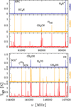 |
Fig. 2 Sample spectra of the three CHEMICO sources. The two spectral windows are extracted from band E0 and band E1. The HMSC G034 is illustrated as blue histograms, the HMPO AFGL and the UCHII G589 as orange and red histograms, respectively. Relevant molecular lines are indicated. |
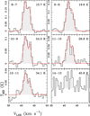 |
Fig. 3 Spectra of the HC3N lines detected towards the HMSC G034. The red curve corresponds to the best fit obtained with MADCUBA using two velocity components. Rotational quantum numbers and Eu of each transition are indicated in the top left and right corners, respectively, in each frame. |
4.1 Line parameters and Tex in the HMSC G034
In G034, as shown by the spectra in Fig. 3, the HC3N lines are well fit by two velocity features with similar FWHM (~1–1.5 km s−1) but different VLSR. The presence of two velocity components in G034 has previously been reported in the HCN isotopologues (Colzi et al. 2018a) and in the NH3 (1,1) and (2,2) inversion transitions (Fontani et al. 2015a). This is due to the two starless cores identified in the ALMA images (Tan et al. 2013) which are not resolved by the IRAM 30m beam (as discussed in Sect. 2). Because both the FWHM and the velocity separation of the two components are similar in all HC3N lines–and the same structure is apparent in C2H, c-C3H2, and C4H– it is natural to interpret these features as two cores embedded within the IRAM 30m beam.
The Tex measured from HC3N and c-C3H2 are 6.8 ± 0.2 K and 4.5 ± 0.4 K, respectively, for the velocity component centred at ~41.3 km s−1, and 6.3 ± 0.5 and 5.7 ± 0.6 K, respectively, for the velocity component centred at ~43.3 km s−1. These values indicate that the emission from these molecules originates from cold and quiescent gas. For CH3CCH, the two velocity components are not resolved, implying that the FWHM of each component is larger than (or comparable to) their velocity separation (2 km s−1). Therefore, the CH3CCH emission is associated with gas that is warmer and more turbulent than that responsible for the HC3N and c-C3H2 emission. Indeed, the Tex measured in CH3CCH is 14.2 ± 1.2 K. This value also agrees with Tk estimated from NH3 (Table 3), indicating that CH3CCH can be in LTE conditions. In contrast, the low Tex values derived from HC3N and c-C3H2 could indicate that these species arise predominantly from a diffuse, low-density envelope, where their lines are likely sub-thermally excited. Because both molecules have large dipole moments (e.g. Shirley 2015), their critical densities are relatively high (≃105−106 cm−3). We also estimated Tex for C2H. However, in this case, the fit to the two velocity features does not converge if both Tex and the total column density are left as free parameters. Therefore, to derive Ntot, we created synthetic spectra by fixing Tex to an integer value between 3 and 15 K, that is, between the cosmic microwave background temperature and the kinetic temperature derived from ammonia (see Table 3), and found that 4 K yields the lowest residuals between the synthetic spectrum and the data.
Excitation temperatures derived with MADCUBA.
Rotational lines of HC3N observable in the four EMIR bands.
4.2 Line parameters and Tex in the HMPO AFGL
Figure 4 shows the HC3N lines detected towards AFGL. Each line is well fitted by two Gaussian features centred at similar velocity: a narrow component with a FWHM of about 3 km s−1, which dominates the profile in the lines with Eu up to ~120 K, and a broad component with FWHM ~7 km s−1, which becomes increasingly prominent in transitions at higher energies. To fit the lines, we used the CDMS spectral parameters, which account for the hyperfine structure. However, the velocity separation among the relevant hyperfine components (i.e. those with an Einstein coefficient of spontaneous emission, Aul, ≥10−5 s−1) is at most ~1 km s−1, which is significantly smaller than the FWHMs of the lines. Figure 4 shows the spectra with the best fit to the two features, as well as their sum. The narrow component is detected up to the J = 32–31 line and has a FWHM comparable to that of all hydrocarbons and HC5N (Table A.2), while the broad component is clearly detected in all transitions of HC3N (Table A.2). The absence of such a broad component in the other molecular species may be due either to an insufficient sensitivity to such fainter emission or because the other species are not appropriate to trace this gas. As shown in Fig. 5, the data for the two velocity components are in excellent agreement with a linear relation, as expected in LTE, but with different Tex. The narrow HC3N component arises from colder gas (Tex~37 K, Table 3) than that associated with the broad component (Tex~125 K). In particular, the Tex of the broad HC3N component agrees, within the errors, with that derived from CH3CN (~117 K, Table 3).
The CH3CN and broad HC3N emissions have very similar FWHM values (~6–7 km s−1, Fig. A.1), and both likely arise from the central region of AFGL, which harbours several millimetre cores, some of which are characterised by hot core-like temperatures (e.g. Zhang et al. 2007; Rivilla et al. 2020b). Rivilla et al. (2020b) also detected an extended outflow, which may contribute to the emission in this broad component. Considering the other Tex estimates, the three simple hydrocarbons c-C3H2, c-C3H, and C2H have Tex between ~14–18 K, while the narrow component of HC3N, HC5N, and CH3CCH have Tex values between ~37–54 K. In general, the lines observed in the IRAM bands are associated with an energy range that is specific to each species: smaller molecules are detected in transitions with lower energy ranges than those observable for the larger molecules. For example, the Eup range of the observable transitions are: C2H is ~4–25 K; C4H is ~17–185 K (~17–304 K in AFGL); HC3N: ~16–203 K (~20–323 K in AFGL); CH3CCH: ~12–696 K (~12–2762 K in AFGL); CH3CN: ~9–670 K (~9–2204 K in AFGL); and HC5N: ~52–684 K (~52–1088 K in AFGL). The ranges of observable and detected transitions for each target are listed in Table 5. However, the lines detected in the CHEMICO dataset span a broad range of overlapping energies (Table 5). Therefore, the differences in Tex derived for hydrocarbons and cyanides depend only partially on the different energy range probed by the observed transitions.
The different Tex values found in AFGL suggest a temperature structure that can be approximated with layers at different temperatures: a cold envelope traced by simple carbon chains with Tk≤20 K; a hot core region with Tk≥100 K; and an intermediate warm region between the cold envelope and the hot core, with Tk~40–50 K. The temperature stratification inferred from our results is illustrated in Fig. 6, where we highlight the difference from the earlier HMSC phase, which is characterised by a uniform temperature. Higher angular resolution observations of the carbon-bearing species studied here are needed to reveal the details of this structure and to quantify the radial extension of each layer.
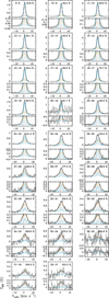 |
Fig. 4 Spectra of the HC3N lines detected towards the HMPO AFGL. In each panel, the best Gaussian fits to the narrow and broad velocity components are shown by the blue and orange curves, respectively; the black curve shows their sum. The panels at the bottom of each spectrum present a zoom on the Y-axis to highlight the high-velocity wings. The rotational quantum numbers and Eu of each transition are indicated in the top-left and top-right corner, respectively. |
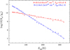 |
Fig. 5 Rotational diagram obtained with MADCUBA towards AFGL (HMPO) from the detected HC3N lines. Blue and red lines indicate the narrow (cold) and broad (hot) velocity features, respectively. The error bars on the y-axis reflect the uncertainties from the fit procedure and the calibration error of 10% on the line integrated intensity. |
Ranges of observed and detected Eu for each species in each source.
Total column densities derived with MADCUBA.
4.3 Line parameters and Tex in the UCHII G589
The lines of HC3N detected towards G589 are shown in Fig. 7. This target exhibits the most intense transitions. As in AFGL, the HC3N lines are best fit by two velocity components: a narrow component (~4 km s−1) and a broad component (~11 km s−1). Figure 8 presents the rotational diagram obtained by fitting these two velocity components separately. The narrower component has an FWHM comparable to that of all hydrocarbons (Table A.2), as in AFGL, and also matches that of CH3CN. This difference indicates that the gas turbulence is progressively increasing. The broad HC3N component is likely associated with the powerful outflow driven by the source(s) embedded in the centre of the UCHII region (Zapata et al. 2020).
4.4 Molecular column densities and fractional abundances
As described in Sect. 3.2, we analysed the spectra using an LTE approach that provided both the Tex and total molecular column densities, Ntot. These values are listed in Table 6. For each detected species, Ntot increases with evolution. The species associated with the highest Ntot enhancement (by two or more orders of magnitude) from the HMSC to the later stages are CH3CN and CH3CCH. From the N(H2) column densities listed in Table 1, we also derived the molecular fractional abundances, X, by dividing Ntot by N(H2). All X are listed in Table 7. Because N(H2) is an average value over an angular region of 28″, and Ntot is computed assuming the emission fills the beam of the CHEMICO observations, X is likewise an average value over 28″. In cases where two velocity components are present, we summed the column densities and obtained X by dividing the sum by N(H2). The most abundant species are C2Hand CH3CCH, both with X of the order 10−9. The remaining species all have X in the range 10−10−10−11. A detailed comparison of the fractional abundances and their relation to the evolutionary stage of the sources is presented in Sect. 5.2.
5 Discussion
5.1 Evolution of the excitation temperatures
Figure 9 presents all Tex derived for the three targets, highlighting trends with evolutionary stage. For each source, hydrocarbons and cyanides are shown separately, with the molecules ordered by increasing number of atoms. The figure also shows Tk in the three targets, as measured from the ammonia (1,1) and (2,2) inversion transitions (Fontani et al. 2015a), which, having critical densities of ~103 cm−3 (e.g. Shirley 2015), are excellent tracers of the kinetic temperature in the moderately dense gas. Several trends are apparent. First, for each tracer, Tex increases from HMSC to the later stages, and in some cases (such as CH3CCH and HC5N) also from the HMPO to the UCHII stage. Second, in each stage, hydrocarbons tend to be associated with lower excitation temperatures than molecules containing a cyanide group, with the exception of CH3CCH. As mentioned in Sect. 4.2, this is in part because hydrocarbons are generally observed in transitions with lower Eu compared to cyanides. However, as highlighted in Table 5, the CHEMICO dataset in principle contains transitions spanning Eu values from ~10 K up to ≫ 100 K for all molecules, except C2H; nevertheless, only those with lower excitation are detected towards small hydrocarbons. Therefore, these species intrinsically trace colder gas more effectively than cyanides. Third, the higher the number of atoms in the molecule, the higher Tex tends to be. In Appendix A, we present a figure similar to Fig. 9 that plots the FWHM of the lines. The FWHM also increases from the earliest to the latest stage, indicating a corresponding increase in the gas turbulence, whereas there is no obvious trend with the number of atoms in the molecule.
Inspecting the Tex changes in more detail, we find that the HMSC G034 consistently exhibits Tex values below 20 K, and these are also smaller than (or comparable to, in the case of CH3CCH) the kinetic temperature derived from ammonia (~15 K). In the HMPO AFGL, a much broader range of Tex is observed: from ~14–18 K in the hydrocarbons c-C3H, c-C3H2, and C2H, up to ~117–125 K in CH3CN and the broad component of HC3N (see Sect. 4.2). A similar range of Tex is derived in the UCHII G589, but with two significant differences. First, the highest temperatures are measured in HC5N, while both CH3CN and the broad component of HC3N both have Tex values < 100 K. Second, in G589, an intermediate Tex of ~20–60 K is absent. These trends indicate an evolution of the temperature structure.
We propose that an envelope with a Tk below or of the order of ~20 K is present in all evolutionary stages. This envelope, well traced by the NH3 inversion transitions at low excitation, experiences a marginal temperature increase with evolution and is preferentially traced by simple hydrocarbons (C2H, c-C3H2, c-C3H). As the embedded protostar(s) heats up the surrounding gas, an inner protostellar envelope becomes warmer than 20 K, and the core is now associated with a Tk gradient. This envelope is traced by larger molecules and cyanide species, and consists of a warm component (Tex~30–60 K) and a hot component (Tex≥100 K), traced respectively by CH3CCH, HC5N and the narrow component of HC3N and CH3CN and the broad component of HC3N. In the UCHII phase, the Tex of the cyanide species and of the complex hydrocarbon CH3CCH increase further. In this late phase, only gas with Tex above 60 K and below 20 K is present. This increased temperature stratification may result from the envelope having had more time to warm up at larger distances from the core centre. Two species, CH3CN and the broad component of HC3N, display a countertrend, showing a decrease in Tex between the HMPO and the UCHII stage. We speculate that this is due to the fact that in the UCHII phase, the innermost part of the hot core–which is the hottest portion of the molecular environment of the nascent protostar(s)–is destroyed by the ionised expanding region. The hot molecular cocoon heated during the HMPO stage becomes reduced to a thinner region in the UCHII stage. Because this thinner hot core is further away from the central nascent star(s), the average Tex is lower than in the intact core in the HMPO stage. The innermost ionised region of G589 is traced in the CHEMICO spectra by hydrogen recombination lines. We detected from the H44α line at ~74.644 GHz to the H29α line at ~256.302 GHz. The FWHM (~60 km s−1) of these lines is consistent with a very hot gas, as confirmed by a preliminary analysis of the excitation temperature of these lines, which exceeds 2000 K. A detailed analysis of these recombination lines will be presented in a forthcoming paper (Fontani et al., in prep.).
A schematic of the temperature structure of G589 based on the CHEMICO data, and the comparison with the earlier evolutionary stages, is shown in Fig. 6.
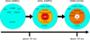 |
Fig. 6 Sketch of the temperature structure in G034, AFGL, and G589. Molecules studied in this work that preferentially trace each layer are indicated. |
Molecular fractional abundances relative to H2.
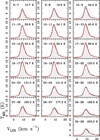 |
Fig. 7 Spectra of the HC3N lines detected towards the UCHII G589. The red curve corresponds to the best fit obtained with MADCUBA using two velocity components. The rotational quantum numbers and the energy of the upper level of each transition are indicated in the top-left and top-right corners, respectively. |
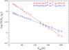 |
Fig. 8 Rotational diagram obtained with madcuba towards G589 (UCHII) from the detected HC3N lines. The blue and red lines indicate the narrow and broad velocity features, respectively. The error bars on the y-axis are calculated as detailed in the caption of Fig. 5. |
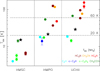 |
Fig. 9 Molecular excitation temperatures. Different colours indicate different species; carbon chains and hydrocarbons are shown in blue, cyan and green and are plotted to the left on the x-axis for each source. Molecules containing the cyanide group are shown in red, orange and pink and are plotted to the right. Black stars indicate the kinetic temperatures as derived from ammonia. For each group, the molecules on the x-axis are ordered from left to right according to increasing number of atoms. |
5.2 Evolution of the fractional abundances
Figure 10 shows the fractional abundances in the three targets, including upper limits for the non-detections. For species with two detected velocity components, abundances were computed by summing the column densities of both components. As in Fig. 9, hydrocarbons and cyanides are displayed separately for each source, with molecules ordered by their number of atoms. For reference, we also plot the fractional abundance of 13CN for cyanide species. In general, the X of the simple species do not vary significantly across the three sources. The only simple molecule associated with a significant increase from the HMSC phase to the later stages is C2H. However, the increase is less than a factor of four and the Tex used to derive Ntot in G034 had to be fixed, as discussed in Sect. 4.1. The only species with clear abundance enhancements with evolution are the two COMs, CH3CCH and CH3CN, whose X values increase by more than an order of magnitude from the HMSC to the HMPO stage. This increase is likely associated with the evaporation of ice mantles from dust grains that releases COMs and their precursors in the gas phase.
Column density ratios for species that are thought to be chemically related (e.g. parent-daughter species, or species formed via similar pathways) are presented in Fig. 11. To simplify the plot, we computed only the ratios associated with the strongest velocity feature in G034 and the narrow velocity features in the AFGL and G589 sources. The only ratio that shows a clear decrease with evolution is C2H/CH3CCH, with C2H being more abundant than CH3CCH in the HMSC and becoming less abundant in the UCHII. Since C2H is a gas-phase precursor of CH3CCH, a decrease could indicate a progressive destruction of C2H into CH3CCH. A tentative decrease is also observed in 13CN/CH3CN, and as CN is also a progenitor of CH3CN, the tentative decrease could be due to the same reason. Ratios that show a significant increase include the CH3CCH/CH3CN ratio between the two COMs, which is enhanced by a factor of ~2.5 from the HMPO to the UCHII stage. The HC3N/HC5N ratio also increases by a factor of 1.7, but this variation is within the error bars. Finally, some ratios show an increase from the HMSC phase to the HMPO phase and then a decrease to the UHCII phase. These include C2H/c-C3H2, 13CN/HC3N, 13CN/HC3N, and 13CN/CH3CN. In particular, the C2H/c-C3H2 ratio increases by an order of magnitude from the HMSC to the HMPO phase. This increase is driven solely by the increasing abundance of C2H, since the abundance of c-C3H2 remains constant (Fig. 10).
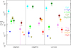 |
Fig. 10 Molecular fractional abundances. As in Fig. 9, hydrocarbons are characterised by blue, cyan, and green colours and are grouped to the left on the x-axis for each source. Molecules with a cyanide group are indicated in red, orange, and pink and are grouped to the right. The molecules on the x-axis are ordered from left to right according to increasing number of atoms (or carbon atoms in the case of equal total atom counts). Upper limits are indicated by downward-pointing triangles. |
5.3 Comparison with other evolution studies
As discussed in Taniguchi et al. (2024), carbon-chain molecules are proposed to be evolutionary indicators in low-mass star-forming cores, although it remains unclear whether this is also the case for high-mass star-forming regions. Based on chemical simulations, Taniguchi et al. (2021) proposed that the C2H/HC5N ratio decreases as temperature increases. In our data, such a decrease is seen between the HMPO and UCHII stages, but not between the HMSC and HMPO stages (Fig. 11). Moreover, the derived ratios, which range from 100 to 300, are between those measured towards the low-mass star-forming core L1527 (~600) and the high-mass cores observed by Taniguchi et al. (2021) (~15). This indicates a large variation in this ratio from one source to another, making it difficult to claim it as an evolutionary indicator.
The ratio between the two cyanopolyynes, HC3N/HC5N, can also potentially be an indicator of evolution. In particular, Fontani et al. (2017) showed that this ratio is sensitive to variations of the cosmic-ray ionisation rate, ζ: a higher ζ value corresponds to a lower HC3N/HC5N ratio. Because protostars are sources of local cosmic rays (e.g. Padovani et al. 2016), ζ close to protostellar objects is expected to be enhanced with respect to that associated with quiescent phases, and therefore the HC3N/HC5N ratio should decrease from the HMSC phase to the later phases. Although we did not detect HC5N in G034, the ratio does not decrease with evolution in our data, perhaps indicating that local cosmic rays do not significantly affect cyanopolyyne abundances on the large angular scales of our observations.
Mininni et al. (2021) found that the abundance of CH3CN is an evolutionary indicator for high-mass star-forming cores, since its abundance increases by more than an order of magnitude between the HMSC and HMPO stages. We confirm this finding and we also confirm the upper limit for the abundance of CH3CNin high-mass starless cores, which is ≤4 × 10⁻¹¹, higher than the value measured toward G034.
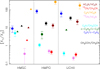 |
Fig. 11 Molecular abundance ratios of chemically related species. As in Fig. 9, hydrocarbons are shown in blue, cyan, and green, and are grouped to the left on the x-axis for each source. containing a cyanide group are indicated in red, orange, and pink. The ratio between the two COMs CH3CCH and CH3CN are indicated in black. Lower limits are indicated by downward-pointing triangles. |
6 Conclusions and outlook
We have presented an overview of the project ‘CHemical Evolution of MassIve star-forming COres’ in which, thanks to an unbiased, full spectral survey of the 3, 2, and 1.2 mm receiver bands of the IRAM 30m telescope, we investigate various aspects of the chemical evolution of three dense cores at different evolutionary stages. The chemical richness is found to increase with evolution in terms of both the species and lines detected. In this first paper, we analyse the carbon-bearing species C2H, c-C3H, c-C3H2, C4H, CH3CCH, HC3N, CH3CN, and HC5N, and derive from them the variation in temperature structure using an LTE approach. Hydrocarbons are associated with Tex lower than those of cyanides. Moreover, the higher the number of atoms in the molecule, the higher Tex. The fractional abundances with respect to H2 show significant enhancement with evolution only for the two COMs, CH3CCH and CH3CN.
We propose that the temperature structure evolves with time as follows. The HMSC stage is characterised by a cold (~20 K) uniform temperature envelope, preferentially traced by simple hydrocarbons (C2H, c-C3H2, c-C3H). Protostellar heating in the HMPO stage creates a temperature structure which can be described as an innermost hot core (Tex≥100 K) traced by CH3CN and the broad components of cyanopolyynes. This hot core is surrounded by a shell at intermediate temperature (30–60 K), traced by CH3CCH, HC5N, and the narrower HC3N component, with a cold extended envelope unaffected by protostellar heating, as in the HMSC stage. Finally, in the UCHII phase, Tex of the cyanide species and of the complex hydrocarbon CH3CCH increase further, and the inner layer with intermediate temperature disappears.
This first study demonstrates the potential of CHEMICO in determining the change in not only the chemical complexity but also the physical structure of the sources with evolution. Followup studies at higher angular resolution will be essential to better investigate the core-scale chemical and physical structure of the three CHEMICO targets, providing key constraints for a direct comparison with chemical models.
Acknowledgements
This work is based on observations carried out under project number [124-20] and [129-21] with the IRAM 30m telescope. IRAM is supported by INSU/CNRS (France), MPG (Germany) and IGN (Spain). We acknowledge the IRAM staff for help provided during the observations. V.M.R. and L.C. acknowledge support from the grant PID2022-136814NBI00 by the Spanish Ministry of Science, Innovation and Universities/State Agency of Research MICIU/AEI/10.13039/501100011033 and by ERDF, UE. V.M.R. also acknowledges support from the grant RYC2020-029387-I funded by MICIU/AEI/10.13039/501100011033 and by “ESF, Investing in your future”, and from the Consejo Superior de Investigaciones Científicas (CSIC) and the Centro de Astrobiología (CAB) through the project 20225AT015 (Proyectos intramurales especiales del CSIC); and from the grant CNS2023-144464 funded by MICIU/AEI/10.13039/501100011033 and by “European Union NextGenerationEU/PRTR”. H.M-C. acknowledges support from the grant JAE-intro (JAEINT-23-01443) from the Consejo Superior de Investigaciones Científicas (CSIC). The research leading to these results has received funding from the European Union’s Horizon 2020 research and innovation program under grant agreement No 101004719 [URP].
Appendix A Fit results for Vp and FWHM
Best fit peak velocity and full width at half maximum obtained with MADCUBA for the lines analysed in this paper. In Fig. A.1 we also plot the FWHM of the lines derived for all molecules in each source. The molecules are plotted as in Fig. 9.
Best-fit Vp.
Best-fit FWHM.
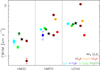 |
Fig. A.1 Line FWHM of all molecules detected in each tracer. Different colours indicate different species as in Fig. 9: carbon chains and hydrocarbons are characterised by blue-cyan-green colours and for each source they are plotted to the left on the x-axis; molecules with the cyanide group are indicated by red-orange-pink colours and are plotted to the right. The black stars are the FWHM derived from ammonia (2,2) (Fontani et al. 2015a). For each group, the molecules on the x-axis are ordered from left to right according to increasing number of atoms. |
Appendix B Spectra of representative lines
Sample spectra of lines representatives of the species analysed in this paper (except HC3N, whose lines are shown in Figs. 3, 4, and 7) for each source.
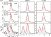 |
Fig. B.1 Spectra of a sample of C2H lines. The red curves are the best LTE fits obtained with MADCUBA. Towards G034, the total fit obtained towards the two velocity components is shown. Quantum numbers and energy of the upper level of the transition are shown in the top left and top right corners, respectively, of the HMSC line plots. |
References
- Adams, F. C. 2010, ARA&A, 48, 47 [NASA ADS] [CrossRef] [Google Scholar]
- André, P., Ward-Thompson, D., & Barsony, M. 2000, in Protostars and Planets IV, eds. V. Mannings, A. P. Boss, & S. S. Russell (Tucson: University of Arizona Press), 59 [Google Scholar]
- Appenzeller, I., & Tscharnuter, W. 1974, A&A, 30, 423 [Google Scholar]
- Arzoumanian, D., Arakawa, S., Kobayashi, M. I. N., et al. 2023, ApJ, 947, L29 [Google Scholar]
- Bonnell, I. A., Vine, S. G., & Bate, M. R. 2004, MNRAS, 349, 735 [Google Scholar]
- Caselli, P., & Ceccarelli, C. 2012, A&ARv, 20, 56 [Google Scholar]
- Carpenter, J. M. 2000, AJ, 120, 3139 [Google Scholar]
- Cernicharo, J., Cabezas, C., Agúndez, M., et al. 2021, A&A, 647, L3 [EDP Sciences] [Google Scholar]
- Coletta, A., Fontani, F., Rivilla, V. M., et al. 2020, A&A, 641, 54 [Google Scholar]
- Colzi, L. 2020, Isotopic fractionation study towards massive star-forming regions across the Galaxy, PhD thesis, Firenze University Press, Premio tesi di dottorato [Google Scholar]
- Colzi, L., Fontani, F., Caselli, P., et al. 2018a, A&A, 609, A129 [NASA ADS] [CrossRef] [EDP Sciences] [Google Scholar]
- Colzi, L., Fontani, F., Rivilla, V. M., et al. 2018b, MNRAS, 478, 3693 [Google Scholar]
- Di Francesco, J., Johnstone, D. K. H., MacKenzie, T., & Ledwosinska, E. 2008, ApJS, 175, 277 [Google Scholar]
- Endres, P., Schlemmer, S., Schilke, P., Stutzki, J., & Müller, H. S. P. 2016, J. Mol. Spectrosc., 327, 95 [NASA ADS] [CrossRef] [Google Scholar]
- Fontani, F., Cesaroni, R., Caselli, P., & Olmi, L. 2002, A&A, 389, 603 [NASA ADS] [CrossRef] [EDP Sciences] [Google Scholar]
- Fontani, F., Palau, A., Caselli, P., et al. 2011, A&A, 529, L7 [NASA ADS] [CrossRef] [EDP Sciences] [Google Scholar]
- Fontani, F., Sakai, T., Furuya, K., et al. 2014, MNRAS, 440, 448 [NASA ADS] [CrossRef] [Google Scholar]
- Fontani, F., Busquet, G., Palau, A., et al. 2015a, A&A, 575, A87 [NASA ADS] [CrossRef] [EDP Sciences] [Google Scholar]
- Fontani, F., Caselli, P., Palau, A., Bizzocchi, L., & Ceccarelli, C. 2015b, ApJ, 808, L46 [NASA ADS] [CrossRef] [Google Scholar]
- Fontani, F., Rivilla, V. M., Caselli, P., Vasyunin, A., & Palau, A. 2016, ApJ, 822, L30 [NASA ADS] [CrossRef] [Google Scholar]
- Fontani, F., Ceccarelli, C., Favre, C., et al. 2017, A&A, 605, A57 [NASA ADS] [CrossRef] [EDP Sciences] [Google Scholar]
- Fontani, F., Vagnoli, A., Padovani, M., et al. 2018, MNRAS, 481, L79 [NASA ADS] [CrossRef] [Google Scholar]
- Fontani, F., Rivilla, V. M., van der Tak, F. F. S., et al. 2019, MNRAS, 489, 45 [Google Scholar]
- Fontani, F., Colzi, L., Redaelli, E., Sipilä, O., & Caselli, P. 2021, A&A, 651, A94 [NASA ADS] [CrossRef] [EDP Sciences] [Google Scholar]
- Fontani, F., Roueff, E., Colzi, L., & Caselli, P. 2023, A&A, 680, A58 [NASA ADS] [CrossRef] [EDP Sciences] [Google Scholar]
- Hernández-Hernández, V., Zapata, L., Kurtz, S., & Garay, G. 2014, ApJ, 786, 38 [Google Scholar]
- Jensen, S. S., Jørgensen, J. K., Kristensen, L. E., et al. 2019, A&A, 631, A25 [NASA ADS] [CrossRef] [EDP Sciences] [Google Scholar]
- Jørgensen, J. K., Belloche, A., & Garrod, R. T. 2020, ARA&A, 58, 727 [Google Scholar]
- Krumholz, M. R. 2015, The Formation of Very Massive Stars, in Very Massive Stars in the Local Universe, ed. J. S. Vink, 412, Astrophysics and Space Science Library [Google Scholar]
- Kutner, M. L., & Ulich, B. L. 1981, ApJ, 250, 341 [NASA ADS] [CrossRef] [Google Scholar]
- Lada, C. J., & Lada, E. A. 2003, ARA&A, 41, 57 [Google Scholar]
- Larson, R. B., & Starrfield, S. 1971, A&A, 13, 190 [NASA ADS] [Google Scholar]
- Loomis, R. A., Burkhardt, A. M., Shingledecker, C. N., et al. 2021, NatAs, 5, 188 [Google Scholar]
- Loren, R. B., Wootten, A., & Mundy, L. G. 1984, ApJ, 286, L23 [Google Scholar]
- Martín, S., Martín-Pintado, J., Blanco-Sánchez, C., et al. 2019, A&A, 631, A159 [Google Scholar]
- McKee, C. F., & Tan, J. C. 2003, ApJ, 585, 850 [Google Scholar]
- Mininni, C., Fontani, F., Rivilla, V. M., et al. 2018, MNRAS, 476, L39 [CrossRef] [Google Scholar]
- Mininni, C., Fontani, F., Sánchez-Monge, Á., et al. 2021, A&A, 653, A87 [NASA ADS] [CrossRef] [EDP Sciences] [Google Scholar]
- Motte, F., Bontemps, S., & Louvet, F. 2018, ARA&A, 56, 41 [NASA ADS] [CrossRef] [Google Scholar]
- Padovani, M., Marcowith, A., Hennebelle, P., & Ferriére, K. 2016, A&A, 590, A8 [NASA ADS] [CrossRef] [EDP Sciences] [Google Scholar]
- Pfalzner, S., Davies, M. B., Gounelle, M., et al. 2015, PhyS, 90, 6 [Google Scholar]
- Pickett, H. M., Poynter, R. L., Cohen, E. A., et al. 1998, J. Quant. Spectr. Rad. Transf., 60, 883 [Google Scholar]
- Rivilla, V. M., Jiménez-Serra, I., Martín-Pintado, J., & Sanz-Forcada, J. 2014, MNRAS, 437, 1561 [Google Scholar]
- Rivilla, V. M., Colzi, L., Fontani, et al. 2020a, MNRAS, 496, 1990 [NASA ADS] [CrossRef] [Google Scholar]
- Rivilla, V. M., Drozdovskaya, M. N., Altwegg, K., et al. 2020b, MNRAS, 492, 1180 [Google Scholar]
- Roueff, E., Parise, B., & Herbst, E. 2007, A&A, 464, A245 [Google Scholar]
- Roueff, E., Gerin, M., Lis, D. C., et al. 2013, JPCA, 117, 9959 [Google Scholar]
- Sabatini, G., Bovino, S., Redaelli, E., et al. 2024, A&A, 692, A265 [NASA ADS] [CrossRef] [EDP Sciences] [Google Scholar]
- Sakai, N., & Yamamoto, S. 2013, Chem. Rev., 113, 8981 [Google Scholar]
- Shirley, Y. L. 2015, PASP, 127, 299 [Google Scholar]
- Shu, F. H., Adams, F. C., & Lizano, S. 1987, ARA&A, 25, 23 [Google Scholar]
- Sipilä, O., & Caselli, P. 2018, A&A, 615, A15 [Google Scholar]
- Suzuki, H., Yamamoto, S., Ohishi, M., et al., 1992, ApJ, 392, 551 [Google Scholar]
- Tan, J. C., Kong, S., Butler, M. J., Caselli, P., & Fontani, F. 2013, ApJ, 779, 96 [Google Scholar]
- Tan, J. C., Beltrán, M. T., Caselli, P., et al. 2014, Protostars and Planets VI, eds. H. Beuther, R. S. Klessen, C. P. Dullemond, & T. Henning (Tucson: University of Arizona Press), 914, 149 [Google Scholar]
- Tan, J. C., Kong, S., Zhang, Y., et al. 2016, ApJ, 821, L3 [Google Scholar]
- Taniguchi, K., Herbst, E., Caselli, P., et al. 2019, ApJ, 881, 57 [Google Scholar]
- Taniguchi, K., Herbst, E., Majumdar, L., et al. 2021, ApJ, 908, 100 [NASA ADS] [CrossRef] [Google Scholar]
- Tychoniec, Ł., van Dishoeck, E. F., van’t Hoff, M. L. R., et al. 2021, A&A, 655, A65 [NASA ADS] [CrossRef] [EDP Sciences] [Google Scholar]
- Taniguchi, K., Majumdar, L., Caselli, P., et al. 2023, ApJS, 267, 4 [CrossRef] [Google Scholar]
- Taniguchi, K., Gorai, P., & Tan, J. C. 2024, Ap&SS, 369, 34 [NASA ADS] [CrossRef] [Google Scholar]
- Yorke, H. W. 1986, ARA&A, 24, 49 [Google Scholar]
- Zapata, L. A., Ho, P. T. P., Fernández-López, M., et al. 2020, ApJ, 902, L47 [Google Scholar]
- Zhang, Q., Hunter, T. R., Beuther, H., et al., 2007, ApJ, 658, 1152 [NASA ADS] [CrossRef] [Google Scholar]
- Zhang, Y., Higuchi, A. E., Sakai, N., et al. 2018, ApJ, 864, 76 [NASA ADS] [CrossRef] [Google Scholar]
- Zinnecker, H., & Yorke, H. W. 2007, ARA&A, 45, 481 [Google Scholar]
MADCUBA is a software developed at the Madrid Center of Astrobiology (CAB, CSIC-INTA) for visualisation and analysis of single spectra and data cubes: https://cab.inta-csic.es/madcuba/
All Tables
All Figures
|
Fig. 1 Scheme of the coarse evolutionary classification for high-mass star-forming cores in HMSCs, HMPOs, and UCHIIs (Colzi 2020, adapted from Motte et al. 2018). |
| In the text | |
|
Fig. 2 Sample spectra of the three CHEMICO sources. The two spectral windows are extracted from band E0 and band E1. The HMSC G034 is illustrated as blue histograms, the HMPO AFGL and the UCHII G589 as orange and red histograms, respectively. Relevant molecular lines are indicated. |
| In the text | |
|
Fig. 3 Spectra of the HC3N lines detected towards the HMSC G034. The red curve corresponds to the best fit obtained with MADCUBA using two velocity components. Rotational quantum numbers and Eu of each transition are indicated in the top left and right corners, respectively, in each frame. |
| In the text | |
|
Fig. 4 Spectra of the HC3N lines detected towards the HMPO AFGL. In each panel, the best Gaussian fits to the narrow and broad velocity components are shown by the blue and orange curves, respectively; the black curve shows their sum. The panels at the bottom of each spectrum present a zoom on the Y-axis to highlight the high-velocity wings. The rotational quantum numbers and Eu of each transition are indicated in the top-left and top-right corner, respectively. |
| In the text | |
|
Fig. 5 Rotational diagram obtained with MADCUBA towards AFGL (HMPO) from the detected HC3N lines. Blue and red lines indicate the narrow (cold) and broad (hot) velocity features, respectively. The error bars on the y-axis reflect the uncertainties from the fit procedure and the calibration error of 10% on the line integrated intensity. |
| In the text | |
|
Fig. 6 Sketch of the temperature structure in G034, AFGL, and G589. Molecules studied in this work that preferentially trace each layer are indicated. |
| In the text | |
|
Fig. 7 Spectra of the HC3N lines detected towards the UCHII G589. The red curve corresponds to the best fit obtained with MADCUBA using two velocity components. The rotational quantum numbers and the energy of the upper level of each transition are indicated in the top-left and top-right corners, respectively. |
| In the text | |
|
Fig. 8 Rotational diagram obtained with madcuba towards G589 (UCHII) from the detected HC3N lines. The blue and red lines indicate the narrow and broad velocity features, respectively. The error bars on the y-axis are calculated as detailed in the caption of Fig. 5. |
| In the text | |
|
Fig. 9 Molecular excitation temperatures. Different colours indicate different species; carbon chains and hydrocarbons are shown in blue, cyan and green and are plotted to the left on the x-axis for each source. Molecules containing the cyanide group are shown in red, orange and pink and are plotted to the right. Black stars indicate the kinetic temperatures as derived from ammonia. For each group, the molecules on the x-axis are ordered from left to right according to increasing number of atoms. |
| In the text | |
|
Fig. 10 Molecular fractional abundances. As in Fig. 9, hydrocarbons are characterised by blue, cyan, and green colours and are grouped to the left on the x-axis for each source. Molecules with a cyanide group are indicated in red, orange, and pink and are grouped to the right. The molecules on the x-axis are ordered from left to right according to increasing number of atoms (or carbon atoms in the case of equal total atom counts). Upper limits are indicated by downward-pointing triangles. |
| In the text | |
|
Fig. 11 Molecular abundance ratios of chemically related species. As in Fig. 9, hydrocarbons are shown in blue, cyan, and green, and are grouped to the left on the x-axis for each source. containing a cyanide group are indicated in red, orange, and pink. The ratio between the two COMs CH3CCH and CH3CN are indicated in black. Lower limits are indicated by downward-pointing triangles. |
| In the text | |
|
Fig. A.1 Line FWHM of all molecules detected in each tracer. Different colours indicate different species as in Fig. 9: carbon chains and hydrocarbons are characterised by blue-cyan-green colours and for each source they are plotted to the left on the x-axis; molecules with the cyanide group are indicated by red-orange-pink colours and are plotted to the right. The black stars are the FWHM derived from ammonia (2,2) (Fontani et al. 2015a). For each group, the molecules on the x-axis are ordered from left to right according to increasing number of atoms. |
| In the text | |
|
Fig. B.1 Spectra of a sample of C2H lines. The red curves are the best LTE fits obtained with MADCUBA. Towards G034, the total fit obtained towards the two velocity components is shown. Quantum numbers and energy of the upper level of the transition are shown in the top left and top right corners, respectively, of the HMSC line plots. |
| In the text | |
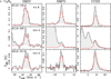 |
Fig. B.2 Same as Fig. B.1 but for c-C3H2. |
| In the text | |
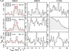 |
Fig. B.3 Same as Fig. B.1 but for C4H. |
| In the text | |
 |
Fig. B.4 Same as Fig. B.1 but for CH3CCH. |
| In the text | |
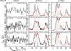 |
Fig. B.5 Same as Fig. B.1 but for CH3CN. |
| In the text | |
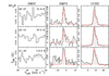 |
Fig. B.6 Same as Fig. B.1 but for HC5N. |
| In the text | |
Current usage metrics show cumulative count of Article Views (full-text article views including HTML views, PDF and ePub downloads, according to the available data) and Abstracts Views on Vision4Press platform.
Data correspond to usage on the plateform after 2015. The current usage metrics is available 48-96 hours after online publication and is updated daily on week days.
Initial download of the metrics may take a while.