| Issue |
A&A
Volume 700, August 2025
|
|
|---|---|---|
| Article Number | A257 | |
| Number of page(s) | 12 | |
| Section | Interstellar and circumstellar matter | |
| DOI | https://doi.org/10.1051/0004-6361/202556046 | |
| Published online | 26 August 2025 | |
Detection of positron in-flight annihilation from the Galaxy
1
Institut de Recherche en Astrophysique et Planétologie, Université de Toulouse, CNRS, CNES, UPS,
9 avenue Colonel Roche,
31028
Toulouse, Cedex 4,
France
2
Laboratoire Univers et Particules de Montpellier, Université de Montpellier, CNRS/IN2P3, Place Eugène Bataillon,
34095
Montpellier Cedex 5,
France
3
Honorary Senior Research Fellow, School of Physics and Astronomy, University of Birmingham,
UK
4
Max-Planck-Institut für extraterrestrische Physik,
Postfach 1603,
85740
Garching,
Germany
★ Corresponding author: This email address is being protected from spambots. You need JavaScript enabled to view it.
Received:
20
June
2025
Accepted:
9
July
2025
Abstract
Context. Although the annihilation of positrons towards the Galactic centre was established more than 50 years ago through the detection of a 511 keV γ-ray line, the origin of the positrons remains unknown. The γ-ray line should be accompanied by continuum emission from positron in-flight annihilation, which, until now, has not been detected.
Aims. We aim to detect positron in-flight annihilation emission, as it provides information on the kinetic energy of the positrons that is key in determining the origin of Galactic positrons.
Methods. We analysed archival data obtained by the COMPTEL instrument on the Compton Gamma-Ray Observatory satellite to search for positron in-flight annihilation emission in the MeV energy range.
Results. Our analysis revealed extended emission in the MeV energy range towards the bulge of the Galaxy, which we attribute to inflight annihilation of positrons produced with kinetic energies of ~2 MeV. The observed spectrum suggests that positrons are produced quasi-mono-energetically, which could occur by the annihilation of dark matter particles with masses of ~3 MeV, or through bulk motion in the jet of the microquasar 1E 1740.7–2942. We furthermore detected a point-like emission component in the MeV energy range towards the Galactic centre that is the plausible low-energy counterpart of the Fermi-LAT source 4FGL J1745.6–2859. The broad band spectrum of the source may be explained by the injection of pair plasma from the supermassive black hole Sgr A* into the interstellar medium, which would also explain the point-like 511 keV line emission component that was discovered by INTEGRAL/SPI at the Galactic centre.
Conclusions. The observed positron in-flight annihilation spectrum towards the Galactic bulge excludes β+ decays from radioactive isotopes, as well as any mechanism producing highly relativistic positrons as the origin of the Galactic bulge positrons.
Key words: stars: black holes / stars: jets / Galaxy: bulge / Galaxy: center / dark matter / gamma rays: ISM
© The Authors 2025
 Open Access article, published by EDP Sciences, under the terms of the Creative Commons Attribution License (https://creativecommons.org/licenses/by/4.0), which permits unrestricted use, distribution, and reproduction in any medium, provided the original work is properly cited.
This article is published in open access under the Subscribe to Open model. This email address is being protected from spambots. You need JavaScript enabled to view it. to support open access publication.
1 Introduction
Observations of the Galactic centre region in the 1970s revealed a 511 keV γ-ray line and continuum emission below 511 keV, which was attributed to two- and three-photon annihilation of thermalised positrons (Johnson et al. 1972; Leventhal et al. 1978). The most recent observations with the Spectrometer on INTEGRAL (SPI) suggest the existence of several positron annihilation emission components, including extended emission from the Galactic bulge that is slightly offset from the Galactic centre, a point-like emission component at the Galactic centre with a characteristic scale of no more than a few hundred parsecs, and extended emission from the Galactic disc with poorly constrained morphology (Bouchet et al. 2010; Skinner et al. 2015; Siegert et al. 2016).
Despite progress on the characterisation of the emission, the origin of the positrons remains an open question, with many possible channels for positron production discussed in the literature (Prantzos et al. 2011; Churazov et al. 2020). The initial kinetic energy of positrons varies strongly between these channels, yet observations of the 511 keV line (or the three-photon continuum emission) probe thermalised positrons that have lost their initial energy due to interactions with ambient medium, erasing the link to their sources. In addition, during the slowdown, positrons can travel substantial distances from the production site (Jean et al. 2009), blurring the link between source distribution and emission morphology.
Positrons may also annihilate in flight before having slowed down, giving rise to Doppler-shifted two-photon continuum emission in the energy interval from mec2/2 to Ep + mec23/2, where mec2 is the rest energy and Ep is the kinetic energy of the positrons. For strongly relativistic positrons, the fraction of in-flight annihilations in the interstellar medium (ISM) may reach several tens of percent, implying that a noticeable flux from positron in-flight annihilation is expected (Agaronyan & Atoyan 1981). Previous attempts to place limits on the positron injection energy include an analysis of INTEGRAL/SPI data that provided non-constraining upper limits (Churazov et al. 2011), and comparisons of expected in-flight γ-ray emission with estimates of observed flux from within a defined patch of sky that place an upper limit of 3–7.5 MeV on the injection energy, depending on the ionisation state of the ISM (Beacom & Yüksel 2006; Sizun et al. 2006).
The latter limits were based on published spectra of Galactic diffuse emission obtained using observations with the Compton Telescope (COMPTEL), an instrument operating on the Compton Gamma-Ray Observatory (CGRO) during 1991–2000. Since COMPTEL did not have direct imaging capabilities, data analysis relied on forward folding of sky distributions with the instrument response function, which allowed the reconstruction of images and spectra in the 0.75–30 MeV energy range (Schönfelder et al. 1993). Furthermore, the instrumental background, which far exceeds any celestial signal, was modelled using an iterative approach, introducing some circularity that makes the resulting images and spectra dependent on the assumed celestial intensity distribution (Bloemen et al. 1999). In particular, emission components that were not explicitly searched for will be suppressed, which implies that upper limits on the positron injection energy derived from published COMPTEL spectra of Galactic ridge emission are not very constraining.
To overcome this limitation, we performed the first dedicated analysis of COMPTEL data that explicitly searched for the signal from positron in-flight annihilation on top of the emission known to be associated with the Galactic ridge. This analysis was carried out as part of an effort to reduce the environmental footprint of astrophysical research by addressing science questions using existing data (Knödlseder et al. 2022a, 2024). We find that such an analysis enables the identification of continuum emission, one component of which has a morphology and spectrum, suggesting that it is due to in-flight annihilation from positrons1.
2 Observations and analysis methods
2.1 Data preparation
For our study, we used COMPTEL data that are publicly available at NASA’s High Energy Astrophysics Science Archive Research Center (HEASARC). Only data recorded before the second reboost of the CGRO spacecraft were used, because the second reboost resulted in a significant increase in the instrumental background at low energies, substantially decreasing the instrument sensitivity (Weidenspointner 1999; Ryan & Collmar 2023). COMPTEL data are split into so-called viewing periods, and our analysis covered 215 viewing periods, starting from viewing period 1.0 and ending with viewing period 616.1, spanning from 16 May 1991 to 18 March 1997.
COMPTEL observed the sky in the energy range from 0.75 MeV to 30 MeV, and we analysed the data using either the full energy range or one of two sub-bands, spanning 0.75–3 MeV and 3–30 MeV, respectively. The sub-bands were split at 3 MeV because around that energy there is a distinct change in the spatial morphology of the emission from the Galactic bulge. We split the data in each energy band into logarithmically spaced energy bins, excluding the 1.7–1.9 MeV energy range that contains the signal from the 1.8 MeV radioactive decay line of 26Al. In total, 16 energy bins were used for the full energy band to accurately determine any spectral cut-offs in the emission, while five and four energy bins were used for the low and high subbands, respectively. There is one more energy bin for the low sub-band compared to the high sub-band due to the exclusion of the 1.7–1.9 MeV interval from the 1.5–2.1 MeV energy bin, which split this energy bin into two.
For each energy bin, events were binned per viewing period into standard COMPTEL data cubes spanned by Compton scatter direction (χ, ψ) and Compton scattering angle ![Mathematical equation: $\[\bar{\varphi}\]$](/articles/aa/full_html/2025/08/aa56046-25/aa56046-25-eq1.png) . Bin sizes of Δχ = Δψ = 1° and
. Bin sizes of Δχ = Δψ = 1° and ![Mathematical equation: $\[\Delta \bar{\varphi}=2^{\circ}\]$](/articles/aa/full_html/2025/08/aa56046-25/aa56046-25-eq2.png) were used throughout the analysis. For each energy bin, we combined data cubes for individual viewing periods into a single data cube that was centred on the Galactic centre and spanned ±120° in Galactic longitude and ±70° in Galactic latitude. This large data cube provides a good contrast between the inner Galactic plane region, which is rich in Galactic γ-ray photons, and high-latitude regions that are essentially free of such photons, allowing a clear separation of γ-ray point sources, Galactic ridge emission, and any excess emission at the Galactic centre. At the same time, the data cube excludes events from the Crab nebula and pulsar which is by far the brightest MeV γ-ray source, avoiding any interference in our analysis by events from this source.
were used throughout the analysis. For each energy bin, we combined data cubes for individual viewing periods into a single data cube that was centred on the Galactic centre and spanned ±120° in Galactic longitude and ±70° in Galactic latitude. This large data cube provides a good contrast between the inner Galactic plane region, which is rich in Galactic γ-ray photons, and high-latitude regions that are essentially free of such photons, allowing a clear separation of γ-ray point sources, Galactic ridge emission, and any excess emission at the Galactic centre. At the same time, the data cube excludes events from the Crab nebula and pulsar which is by far the brightest MeV γ-ray source, avoiding any interference in our analysis by events from this source.
2.2 Data analysis
All data analysis was performed using version 2.1.0 of the ctools (Knödlseder et al. 2016) and GammaLib (Knödlseder 2011) software packages. We analysed the data by adjusting model components to the observed events using a maximum-likelihood method. Each model component consists of parametrised spatial and spectral models, which we fitted jointly to the data cubes for all energy bins in a given energy band. We used the comlixfit script for model fitting, which derives a model of the instrumental background event distribution in the data cubes while simultaneously adjusting the parameters of the celestial model components (Knödlseder et al. 2022b). The most critical parameter of the algorithm is Nincl, which specifies the number of ![Mathematical equation: $\[\bar{\varphi}\]$](/articles/aa/full_html/2025/08/aa56046-25/aa56046-25-eq3.png) layers of the three-dimensional data cubes used to estimate the background model. As demonstrated by Knödlseder et al. (2022b), large values of Nincl conserve the celestial source fluxes but may lead to substantial residuals attributed to an inadequate modelling of the instrumental background event distribution. Smaller values of Nincl reduce these residuals, but do so at the expense of suppressing some of the source flux and detection significance. To minimise background residuals while still conserving source fluxes, we used Nincl = 11 in this study. We used the BGDLIXF algorithm for background modelling, which is an evolution of the BGDLIXE algorithm described in Knödlseder et al. (2022b) and which properly treats background event rate variations between and within viewing periods (see Appendix A).
layers of the three-dimensional data cubes used to estimate the background model. As demonstrated by Knödlseder et al. (2022b), large values of Nincl conserve the celestial source fluxes but may lead to substantial residuals attributed to an inadequate modelling of the instrumental background event distribution. Smaller values of Nincl reduce these residuals, but do so at the expense of suppressing some of the source flux and detection significance. To minimise background residuals while still conserving source fluxes, we used Nincl = 11 in this study. We used the BGDLIXF algorithm for background modelling, which is an evolution of the BGDLIXE algorithm described in Knödlseder et al. (2022b) and which properly treats background event rate variations between and within viewing periods (see Appendix A).
We modelled the celestial γ-ray emission using components for the in-flight positron annihilation emission, ten point sources previously detected in MeV γ-rays in the examined region (see Appendix B), and components for Galactic ridge and cosmic γ-ray emission. We modelled the spectra of all point sources and the cosmic γ-ray background using power laws, while we used more elaborate spectral forms for the other components. We adjusted the spectral parameters of all components during model fitting, with the exception of the cosmic γ-ray background component, which is spatially isotropic and therefore cannot be distinguished from the instrumental background through spatial model fitting. We therefore fixed this component to the spectrum I(E) = 1.12 × 10⁻⁴(E/5 MeV)−2.2 ph cm−2 s−1 MeV−1 sr−1, as suggested by Weidenspointner (1999).
The Galactic ridge emission at energies in the MeV range is believed to originate primarily from diffuse inverse-Compton (IC) emission of cosmic-ray electrons, yet contributions from unresolved source populations cannot be excluded (Bloemen et al. 1999; Strong & Moskalenko 2000). To avoid any biases from an assumed spatial distribution of Galactic diffuse emission, and to allow for the possible presence of unresolved point sources, we implemented an empirical model using two-dimensional (2D) asymmetric Gaussian functions for the spatial distribution. For the low- and high-energy band fits, we used a single 2D asymmetric Gaussian function as the spatial model, with a power-law spectral model for which we adjusted the prefactor and index. For the full-energy band fits we used two 2D asymmetric Gaussian functions to accommodate different spatial morphologies of the Galactic ridge emission at low and high energies. We modelled the spectra of both components using log-parabola functions, adjusting the prefactor, the index, and the curvature during the fit.
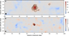 |
Fig. 1 Test statistic (TS) maps in the 0.75–3 MeV (a) and 3–30 MeV (b) energy bands. The significance, expressed in Gaussian sigma, corresponds to |
![Mathematical equation: $\[\sqrt{\mathrm{TS}}\]$](/articles/aa/full_html/2025/08/aa56046-25/aa56046-25-eq4.png)
3 Results
3.1 Excess emission maps
We searched for excess emission towards the Galactic bulge region by generating test statistic (TS) maps spanning 200° × 50° in Galactic longitude and latitude around the Galactic centre, following the method described in Knödlseder et al. (2022b). We derived the maps by fitting a point-source model to a 1° grid of source locations, on top of a reference model that includes all known γ-ray sources in the region of interest, comprising Galactic ridge emission, point sources, and cosmic γ-ray background, as well as a description of the instrumental background. As the morphology of the excess emission changes within the COMPTEL energy range, we derived separate maps for the 0.75–3 MeV and 3–30 MeV energy bands, which are shown in Fig. 1.
The TS map for the 0.75–3 MeV energy band reveals significant excess emission towards the Galactic centre, with a morphology that is clearly extended and an emission peak that appears slightly offset towards negative longitude. This is the first report of MeV excess emission from the Galactic bulge, and the resemblance of the TS map to the initial 511 keV line emission maps from INTEGRAL/SPI (Knödlseder et al. 2005) is striking. The map shows few features outside the Galactic bulge excess, indicating that the reference model adequately describes the emission from the Galactic ridge and the known point sources within the analysis region. Significant excess emission is also seen in the 3–30 MeV energy band, with a point-like morphology located at the Galactic centre. Besides the Galactic centre source, there is no other significant excess in the map.
To illustrate that the excess emissions are not artefacts of the Galactic ridge emission model and that they persist under changes of the model, we show in Fig. 2 TS maps derived using alternative Galactic ridge emission models. Galactic ridge emission at energies in the MeV range is believed to originate primarily from diffuse IC emission of cosmic-ray electrons (Strong et al. 2000); hence, we replaced the 2D asymmetric Gaussian functions in our reference model with either an IC map employed in past COMPTEL data analysis (designated by ‘COMPASS’; Youssefi & Strong 1991) or an IC map derived using GALPROP (Ackermann et al. 2012). The resulting TS maps confirm extended 0.75–3 MeV excess emission towards the Galactic bulge and the point-like 3–30 MeV excess at the Galactic centre. The 0.75–3 MeV excess is detected at significance levels exceeding those for the reference model and now shows a slightly elongated morphology along the Galactic plane. This suggests that the IC maps do not fully account for all Galactic ridge emission, which is confirmed by the presence of significant residual Galactic disc emission in the 3–30 MeV maps at negative Galactic longitudes. The IC maps therefore do not accurately describe the observed Galactic ridge emission, which was the principal motivation for employing 2D asymmetric Gaussian functions in our reference model to better describe its morphology.
Past COMPTEL data analyses partially compensated for these inadequacies by incorporating a map of Bremsstrahlung emission into the Galactic ridge emission model, although it remains unclear whether the Bremsstrahlung process actually contributes to the observed emission or instead mimics a population of unresolved point sources (Bloemen et al. 1999; Strong & Moskalenko 2000). Including Bremsstrahlung maps in the analysis (using maps derived for COMPTEL or using GALPROP; Strong et al. 1993; Ackermann et al. 2012) results in TS maps with fewer residual features outside the Galactic bulge compared to the maps derived using only the IC templates, although they do not achieve the low residual levels obtained with the reference model. The 0.75–3 MeV excess is confirmed, further demonstrating that its existence does not depend on the choice of Galactic ridge emission model. The significance of the 3–30 MeV Galactic centre excess is more sensitive to the choice of Galactic ridge emission model, falling below 3σ when a combination of GALPROP IC and Bremsstrahlung maps is used. This decrease is related to a peak in the Bremsstrahlung map towards the Galactic centre, which reflects the high ISM density in the central molecular zone (CMZ). The flux in the 3–30 MeV Galactic centre excess may therefore be overestimated in our reference model.
3.2 Characterisation of excess emissions
To characterise the excess emissions, we added a 2D Gaussian spatial model with a power-law spectrum to the reference model and fitted its free parameters (position, extension, power-law prefactor, and index) jointly with all free parameters of the reference model. This resulted in a full width at half maximum (FWHM) of 7.8° ± 1.8° for the emission in the 0.75–3 MeV energy band, with a centroid at l = −1.4° ± 0.8° and b = −0.2° ± 0.9°, slightly offset from the Galactic centre towards negative longitudes. The quoted uncertainties are statistical and correspond to a confidence level of 68%. Notably, these parameters correspond closely to those of the narrow bulge component of the 511 keV line emission model of Skinner et al. (2015), which has a FWHM of 7.5° and is centred on l = −1.15° and b = −0.25° (see also below). The model has a fitted 0.75–3 MeV flux of (21.2 ± 3.7) × 10−5 photons cm−2 s−1 and a TS value of 65.5, corresponding to a detection significance of 8.1σ. Using more complex models, such as elliptical Gaussians with fixed or free position angle, did not lead to significant fit improvements. For the 3–30 MeV energy band, the emission is unresolved, with a FWHM < 3.6° (95% confidence level) and a centroid at l = −0.1° ± 0.6° and b = 0.7° ± 0.6°. The model has a fitted 3–30 MeV flux of (3.6 ± 0.9) × 10−5 photons cm−2 s−1 and a TS value of 26.9, corresponding to a detection significance of 5.2σ.
To search for time variability of the excess emissions, we divided the full observing period into four equally long time intervals and fitted the excess emission for each of the intervals by fixing the spatial model parameters to the values that we obtained above. The results of this analysis are summarised in Table 1, along with the fluxes derived for the full observing period. The fluxes in each time interval are compatible within uncertainties with those for the full period, revealing no time variability in the excess emissions.
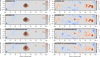 |
Fig. 2 TS maps for the 0.75–3 MeV (left) and 3–30 MeV (right) energy bands for different Galactic ridge emission models (see text). |
Fitted excess fluxes, in units of 10−5 photons cm−2 s−1, for different time intervals.
3.3 Comparison with the morphology of the 511 keV line emission
Motivated by the morphological similarity between the extended 0.75–3 MeV emission and the 511 keV line emission from the Galactic bulge, we compared the COMPTEL data in both energy bands to a model of the Galactic bulge 511 keV line emission derived by Skinner et al. (2015) from ten years of INTEGRAL/SPI data. This model is the most detailed developed to date and is comprised of three components that include a point source located at the position of Sgr A* and two symmetric Gaussians modelling the narrow and broad bulge emission components. While the broad component is centred on the Galactic centre, the narrow component is offset from the Galactic centre towards l = −1.15° and b = −0.25°. Table 2 presents the TS values and fluxes obtained for the three model components in both energy bands. For components that were not detected, 95% confidence-level upper flux limits were derived.
The log-likelihood value of the fits in both energy bands were comparable to those obtained by fitting a simple 2D Gaussian model, implying that the model of Skinner et al. (2015) contains all components needed to explain the excess emissions seen by COMPTEL. In the 0.75–3 MeV energy band, the ‘Core’ component of Skinner et al. (2015) was not detected, and most of the flux was attributed to the ‘Narrow bulge’ component. This contrasts the situation for the 511 keV line emission, where Skinner et al. (2015) found that ~70% of the flux is attributed to the ‘Broad bulge’ component, implying that the 0.75–3 MeV excess emission is less extended compared to the 511 keV line emission. In the 3–30 MeV energy band, all emission is attributed to the ‘Core’ component of Skinner et al. (2015), while no emission is attributed to the bulge components, for which only upper limits could be derived. This is consistent with Figs. 1 and 2, which show no indication of extended emission in the 3–30 MeV energy band, confirming the drastic change in emission morphology at approximately 3 MeV.
TS values and fitted fluxes, in units of 10−5 photons cm−2 s−1, for the three-component model of Skinner et al. (2015) of the Galactic bulge 511 keV line emission.
3.4 Spectral energy distributions
To advance our understanding of the nature of the excess emissions, we derived spectral energy distributions (SEDs) for extended and point-like components by performing model fits over the full 0.75–30 MeV COMPTEL energy range. To separate the SED of the extended component from that of the point-like component, we jointly fitted two models on top of the reference model: a 2D symmetric Gaussian shape to model the extended low-energy emission (hereafter the ‘Bulge component’) and a point source to model the point-like high-energy emission (hereafter the ‘Core component’). We fixed the spatial parameters of both components to the values found in the analysis of the 0.75–3 MeV and 3–30 MeV energy bands. The spectra of both components were modelled using so-called ‘bin functions’, where piecewise power laws with fixed spectral index Γ = 2 and free intensity were logarithmically spaced over the full energy range. In this way, the number of spectral points in the SED becomes independent of the number of energy bins used for the data. We chose eight spectral points for the Bulge component and three spectral points for the Core component to capture the spectral evolutions as well as possible while assuring signal detection over as broad an energy range as possible. In addition, we performed fits where the bin functions were replaced by analytical spectral laws, such as power laws, exponentially cut-off power laws, and log-parabola spectra, to study the spectral evolution of the excess emissions independently of any spectral binning. We translated uncertainties in the spectral parameters into uncertainty bands that account for the covariance between the spectral parameters of the Bulge and Core components.
The resulting SEDs and fitted analytical spectra for the Bulge and Core components are shown in Fig. 3. As expected from the excess emission maps, the Bulge component dominates the emission at low energies. Above ~2 MeV the energy flux starts to drop, and above ~3 MeV only upper flux limits could be derived, consistent with the absence of extended emission towards the Galactic bulge region in the 3–30 MeV excess emission map. The Bulge component is well fitted by either an exponentially cut-off power law or a log-parabola spectrum. For the latter, we derived 0.75–30 MeV photon and energy fluxes of (1.5±0.4) × 10−4 photons cm−2 s−1 and (3.4±0.9) × 10−10 erg cm−2 s−1. For a source situated at the distance of the Galactic centre (8.2 kpc; GRAVITY Collaboration 2019), the flux corresponds to a luminosity of (2.7±0.7) × 1036 erg s−1, which is approximately 10% of the annihilation luminosity from thermalised positrons (Churazov et al. 2020).
The Core component shows a distinctively different SED, with a steady rise of the energy flux over the COMPTEL energy range, compatible with a simple power law. We derived 0.75–30 MeV photon and energy fluxes of (5.9±2.4) × 10−5 photons cm−2 s−1 and (5.7±1.2) × 10−10 erg cm−2 s−1, corresponding to a luminosity of (4.5±1.0) × 1036 erg s−1 for a source at the distance of the Galactic centre.
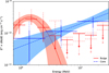 |
Fig. 3 Spectral energy distributions and fitted spectral laws for the Bulge and Core components. Systematic uncertainties related to different modelling of the Galactic ridge emission are shown as light dashed vertical bars. For upper limits, we show the smallest and largest values obtained under variation of the Galactic ridge emission model as faint dashed arrows. |
3.5 Comparison to expected positron in-flight annihilation spectra
As the morphology of the Bulge component suggests positron in-flight annihilation as the possible origin of the emission, we investigated whether the spectrum is also compatible with such a scenario and whether conclusions can be drawn about the underlying positron sources. For this purpose, we modelled the γ-ray emission from a population of energetic positrons interacting with electrons in the ISM, following the prescriptions of Beacom & Yüksel (2006), Sizun et al. (2006), and Prantzos et al. (2011). While these prescriptions are limited to the case of stationary injection of mono-energetic positrons into the ISM, we extended the formalism to arbitrary injection spectra. Following Beacom & Yüksel (2006), we normalised the resulting γ-ray intensities to be in units of equivalent 511 keV line flux Φ511, using the observed positronium fraction of fPs = 0.967 (Jean et al. 2006), so that when fitting the models to the COMPTEL data, the model normalisation is given in units of Φ511 (see Appendix C).
Figure 4 shows model spectra for the Bulge and Core components resulting from a joint fit of both components to the data over the 0.75–30 MeV energy band. The Bulge component was modelled using a 2D Gaussian spatial model with parameters fixed to the values determined from the 0.75–3 MeV energy band, combined with a spectral positron in-flight annihilation model for which Φ511 was fitted. Additional free parameters include the injection energy, Ep, for mono-energetic models (panels a and b), the maximum injection energy, Emax, and the spectral index, Γ, for the power-law particle injection spectra (panels c and d). In all fits, the Core component was modelled by a point source located at the position obtained in the 3–30 MeV energy band with a power-law spectrum.
The Bulge component is best fitted by a spectral model that assumes the stationary injection of mono-energetic positrons with kinetic energies of 2.0 ± 0.1 MeV into the ISM (panel a). The injection energy increases slightly to 2.1 ± 0.1 MeV in the case of dark matter annihilation, owing to the additional internal Bremsstrahlung emission component (panel b). Both models result in a TS value of 15.3 for the Bulge component, corresponding to a detection significance of 3.9σ for the Bulge component on top of a model comprising only the Core component. An equally good fit is obtained by assuming the injection of positrons with a power-law spectrum ![Mathematical equation: $\[N(E_{p}) \propto E_{p}^{-\Gamma}\]$](/articles/aa/full_html/2025/08/aa56046-25/aa56046-25-eq5.png) of kinetic energies that is cut off at a maximum energy of 2.2 ± 0.7 MeV, resulting in a TS value of 15.1 for the Bulge component (panel c). The fitted power-law slope of Γ ~ −7 is extremely hard, resulting in a spectrum that is heavily peaked towards the maximum kinetic energy, implying that it is quasi mono-energetic. Forcing the slope of the injection spectrum to Γ = 2 and setting Emax = 50 MeV results in a marginal TS value of 1.0 for the Bulge component (panel d), demonstrating that the injection of a broad-band spectrum of positrons into the ISM to explain the Bulge component is strongly excluded by the COMPTEL data. Finally, fitting the expected spectra for positrons produced by the β+ decays of 22Na (panel e), 26Al (panel f), 44Sc (panel g), and 56Co (panel h) results in TS values below the 3σ significance level for the Bulge component, essentially because these spectra cut off at energies below the observed cut-off of the Bulge component.
of kinetic energies that is cut off at a maximum energy of 2.2 ± 0.7 MeV, resulting in a TS value of 15.1 for the Bulge component (panel c). The fitted power-law slope of Γ ~ −7 is extremely hard, resulting in a spectrum that is heavily peaked towards the maximum kinetic energy, implying that it is quasi mono-energetic. Forcing the slope of the injection spectrum to Γ = 2 and setting Emax = 50 MeV results in a marginal TS value of 1.0 for the Bulge component (panel d), demonstrating that the injection of a broad-band spectrum of positrons into the ISM to explain the Bulge component is strongly excluded by the COMPTEL data. Finally, fitting the expected spectra for positrons produced by the β+ decays of 22Na (panel e), 26Al (panel f), 44Sc (panel g), and 56Co (panel h) results in TS values below the 3σ significance level for the Bulge component, essentially because these spectra cut off at energies below the observed cut-off of the Bulge component.
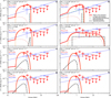 |
Fig. 4 Expected γ-ray spectra for positrons in flight (red lines), including contributions from in-flight annihilation (dashed orange lines), Bremsstrahlung (dotted brown lines), and internal Bremsstrahlung (dash-dotted green line). Positron injection spectra are shown as dash-dotted black lines. Model spectra are shown for stationary injection of mono-energetic positrons (a), dark matter annihilation (b), stationary injection of positrons obeying a power-law spectrum of slope Γ and maximum energy Emax (c, d), and β+ decays of radioactive isotopes (e–h). The power-law spectra of the jointly fitted Core component are shown as light blue lines. The SEDs of the Bulge and Core components, replicated from Fig. 3, are shown as red and light blue data points for visual comparison. Fitted parameters for the Bulge component and TS values for the Bulge and Core components are given in each panel. |
4 Discussion
4.1 Possible origin of the Bulge component
The resemblance of the morphology of the Bulge component to that of the 511 keV line bulge emission is striking. Both emissions are extended, with comparable sizes, and exhibit an emission centroid that is slightly offset from the Galactic centre towards negative longitudes. The characteristics of this emission morphology are unique, having no counterpart in the gas components or stellar populations of the Galaxy (Prantzos et al. 2011). Consequently, we suggest that the Bulge component most plausibly originates from positron in-flight annihilation.
After production, positrons do not annihilate immediately owing to the relatively low densities of the ISM (Prantzos et al. 2011). Survival times may range from ~103 years in the dense regions around the Galactic centre to several times 105 years in the Galactic disc, during which time positrons will propagate away from their sources. As positron in-flight annihilation occurs before positron thermalisation, the in-flight annihilation emission should have a more compact morphology compared with the 511 keV line emission. However, because in-flight annihilation is most probable after positrons have lost much of their initial energy, it tends to occur after positrons have travelled substantial distances. Hence, the extension of the emissions may not differ significantly. Comparison of the morphology of the Bulge component with morphology models of 511 keV line emission (cf. Table 2) suggests that the Bulge component is more compact than the 511 keV line emission, in line with expectations if the Bulge component originates from positron in-flight annihilation.
The SED of the Bulge component is difficult to explain with cosmic-ray-induced IC or Bremsstrahlung emissions, as these have broad-band spectra spanning many decades in energy and do not show the observed spectral cut-off (Strong et al. 2000). As illustrated in Fig. 4, the Bulge component is best fitted by a quasi mono-energetic injection of positrons with kinetic energies of ~2 MeV into the ISM. This excludes radioactive β+ decays as noticeable contributors to the Bulge component, since their positron spectra are limited to sub-MeV energies, producing γ-ray spectra that cut off below ~1 MeV. Some reacceleration of β+ decay positrons would be required to increase the injection energies to the observed values; however, it is unclear how such a scenario would produce the quasi mono-energetic energy distribution observed for the Bulge component. Scenarios injecting highly relativistic positrons into the ISM – such as cosmic-ray secondaries produced from π+ decays, normal pulsars, millisecond pulsars, and magnetars – are also excluded as positron sources of the Bulge component, since they would lead to a positron in-flight annihilation spectrum extending to much higher energies.
One proposed source producing mono-energetic positrons with the required kinetic energies is the annihilation of light dark matter particles (Boehm et al. 2004). If such particles exist, their annihilation would result in MeV γ-ray emission dominated by positron in-flight annihilation, with additional smaller contributions from internal and external Bremsstrahlung (Beacom & Yüksel 2006; Sizun et al. 2006; Boehm & Uwer 2006). Fitting the expected spectra to the COMPTEL data suggests a dark matter particle mass of ~3 MeV and implies a 511 keV line flux of (1.5±0.3) × 10−3 photons cm−2 s−1. For a source at the distance of the Galactic centre, this flux corresponds to a positron production rate of (2.3±0.5) × 1043 s−1. This is at the upper end of the range of positron annihilation rates inferred from INTEGRAL/SPI 511 keV line data for the bulge component, but compatible with estimates for the entire Galaxy, including the bulge and a putative disc component (Churazov et al. 2020). This may indicate that some positrons escape from the bulge into the disc region, where they thermalise and finally annihilate, producing the 511 keV line disc emission.
The offsets of the centroids of the bulge emissions towards negative longitudes, however, present a challenge for the dark matter scenario. Offsets could, in principle, be explained by ISM overdensities that enhance positron annihilation, yet the ISM distribution towards the Galactic centre is offset towards positive, not negative, longitudes (Ferrière 2008). This excludes the ISM distribution as an explanation and suggests that the offset is instead related to the positron injection site. While it cannot be excluded that the barycentre of the dark matter particles is offset from the dynamical centre of the Galaxy (Kuhlen et al. 2013), tidal forces produced by baryons, which dominate the gravitational potential near the Galactic centre, should remove such an offset within ~10 million years (Gorbunov & Tinyakov 2013).
Another issue with the dark matter hypothesis is the high ISM density in the CMZ around the Galactic centre (Ferrière 2008), which implies that any positron injected into that zone will annihilate within a few thousand years and will not propagate more than a few tens of parsecs at most. Therefore, positron sources located within the CMZ should lead to strongly peaked annihilation emission towards the Galactic centre, with an angular extent less than the ~2° size of the CMZ (Alexis et al. 2014). Since the Bulge component does not show such a compact source (cf. Table 2), it is unlikely that the source giving rise to the extended Bulge component is located in the immediate vicinity of the Galactic centre. This excludes, in particular, Sgr A* as the main positron source for the Bulge component.
A candidate positron source seen near the Galactic centre, but located at the edge or possibly even outside the CMZ, is the microquasar 1E 1740.7–2942 (Luque-Escamilla et al. 2015; Tetarenko et al. 2020). Intriguingly, its position coincides with the centroid of the 511 keV line bulge emission (Skinner et al. 2015) as well as with the centroid of the Bulge component. 1E 1740.7–2942 has been dubbed the ‘Great Annihilator’ owing to past reports of transient positron annihilation features in its spectrum (Bouchet et al. 1991; Sunyaev et al. 1991). Although these observations have been questioned (Prantzos et al. 2011), 1E 1740.7–2942 remains a plausible source of positrons, since microquasars may produce positrons in the inner region of the accretion disc or hot corona, which are then channelled into the ISM through their jets (Guessoum et al. 2006). While microquasars are variable sources, their variability occurs on timescales much shorter than the positron lifetime in the ISM. Hence, regardless of whether positrons are produced during outbursts or rather continuously, microquasars should act as steady sources of positron annihilation. The time-averaged jet power of 1E 1740.7–2942 is estimated to be (0.7–3.5) × 1037 erg s−1 (Tetarenko et al. 2020), which is sufficient to produce the observed positron annihilation luminosity of the Bulge component if the jet is composed of a pure pair plasma. The plasma’s bulk motion will inject positrons with relatively constant kinetic energies into the ISM (Heinz & Sunyaev 2002), which would explain the quasi mono-energetic positron spectrum that we inferred for the Bulge component. Bulk Lorentz factors of microquasar jets are uncertain, but values of up to Γ ~ 4 are discussed in the literature (Luque-Escamilla et al. 2015; Zdziarski et al. 2022). This would correspond to kinetic energies of ~1.5 MeV, which is close to the value inferred for the Bulge component. After injection, positrons propagate along magnetic field lines away from the source while slowing down due to scattering on gas particles and possibly plasma waves (Jean et al. 2009), giving rise to extended positron annihilation emission whose morphology depends on the magnetic field configuration and the density and dynamics of the ISM (Alexis et al. 2014). While some positrons may annihilate in the CMZ, the strong turbulence in the inner Galaxy, combined with gas outflows (Sarkar 2024), may transport positrons away from the source, leading to the observed extended emission feature (Panther et al. 2018).
The obvious question in this scenario is why no positron annihilation emission is observed around other microquasars. The object 1E 1740.7–2942 is unique among microquasars, remaining persistently in the bright outburst state and accreting near peak luminosity most of the time, which are properties shared only with GRS 1758–258 (Tetarenko et al. 2016). However GRS 1758–258 has a lower jet power (Tetarenko et al. 2020) and is located further away from the Galactic centre, placing it in a less dense region of the ISM. Lower ISM densities imply larger positron propagation distances and higher escape fractions, reducing positron annihilation emission intensities. The combination of a powerful positron source located in a dense ISM region could explain why 1E 1740.7–2942 is the only currently detectable microquasar source of positrons.
4.2 Possible origin of the Core component
The SED of the Core component differs significantly from that of the Bulge component (cf. Fig. 3), suggesting distinct origins. It is nevertheless intriguing that both the 511 keV line and MeV continuum emissions exhibit a compact component at the Galactic centre (Skinner et al. 2015; Siegert et al. 2016), raising the question of whether the Core component is also related to positron annihilation. A central component could, in principle, be produced by the enhanced gas density in the CMZ, leading to enhanced positron annihilation emission; however, in that scenario, the SEDs of the Core and Bulge components would be similar.
The missing link is likely the compact source in the GeV energy range, 4FGL J1745.6–2859, observed by Fermi-LAT at the Galactic centre (Malyshev et al. 2015; Abdollahi et al. 2022; Cafardo et al. 2021). This is by far the brightest Fermi-LAT source in the field of the Core component. As illustrated in Fig. 5, the SEDs of the Core component and 4FGL J1745.6–2859 connect rather well, making the Fermi-LAT source the most plausible high-energy counterpart of the Core component. While the 8.8–30 MeV flux of the Core component is slightly in excess of a smooth spectral connection, the modelling of the Galactic ridge emission introduces some systematic uncertainties in the flux levels. This also applies for the Fermi-LAT low-energy fluxes (Malyshev et al. 2015; Abdollahi et al. 2022; Cafardo et al. 2021). Within these uncertainties, the connection between the two SEDs is satisfactory.
4FGL J1745.6–2859 is a non-variable γ-ray source of unknown nature. However, the production of relativistic hadrons or leptons by Sgr A* is generally invoked to explain its GeV emission (Cafardo et al. 2021). Fig. 5 shows the γ-ray spectrum arising from the continuous injection of a relativistic pair plasma into the ISM at the Galactic centre, with a particle spectrum slope Γ of 2.1 and maximum energy of 1 TeV. This model satisfactorily explains the observed SEDs of the Core component and 4FGL J1745.6–2859, while simultaneously producing a 511 keV line emission of 10−4 photons cm−2 s−1. This flux corresponds to the observed flux for the central 511 keV line emission component (Skinner et al. 2015; Siegert et al. 2016). In such a model, the γ-ray emission would primarily be IC emission due to the high radiation field at the Galactic centre (Kusunose & Takahara 2012), with contributions from positron in-flight annihilation and Bremsstrahlung at low energies. The high radiation field and large ISM density at the Galactic centre imply that positrons will thermalise quickly and propagate less, explaining the compact appearance of the source. Once thermalised, positron annihilation will lead to 511 keV line emission which produces the central component observed in the INTEGRAL/SPI data (Skinner et al. 2015; Siegert et al. 2016).
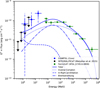 |
Fig. 5 Modelling the SED of the Core component. The Core component SED is shown together with the SED of the Fermi-LAT source 4FGL J1745.6–2859 (Abdollahi et al. 2022) and upper limits from INTEGRAL/PICsIT (Malyshev et al. 2015) (black). A best-fitting model for a pair plasma injected by Sgr A* is shown as a solid blue line. Contributions to the model from IC (dotted line), positron in-flight annihilation (dashed line), and Bremsstrahlung (dash-dotted line) emissions are also shown. |
5 Conclusions
By analysing archival data from the COMPTEL telescope we establish the presence of MeV excess emission on top of the Galactic ridge γ-ray emission towards the Galactic centre region. The morphology of this excess emission changes markedly within the COMPTEL 0.75–30 MeV energy range, switching from an extended emission morphology below ~3 MeV to a point-like appearance above that energy. A spectral analysis reveals the presence of two distinct excess emission components towards the Galactic centre.
We plausibly identify the first component to originate from positron in-flight annihilation and reveal that its spectrum matches a scenario in which Galactic bulge positrons are produced by dark matter annihilation (Beacom & Yüksel 2006; Sizun et al. 2006; Boehm & Uwer 2006). If this scenario applies, we estimate the rest mass of the dark matter particles to be ~3 MeV. The only other candidate source, besides dark matter annihilation, that satisfies the observations is positron injection through the jets of the microquasar 1E 1740.7–2942; however, it remains unclear whether that scenario can satisfactorily explain the extended morphology of the emission. Thus, the precise origin of positrons in the Galactic bulge remains unknown, but our observations exclude many sources previously proposed (Prantzos et al. 2011). In particular, β+ decays from radioactive isotopes and sources producing highly relativistic positrons, such as cosmic-ray secondaries produced from π+ decays, normal pulsars, millisecond pulsars, and magnetars, can be clearly discarded as primary source of Galactic bulge positrons.
We plausibly identify the second component as the low-energy counterpart of the Fermi-LAT point source 4FGL J1745.6–2859, which coincides with the location Sgr A*. While the production of relativistic hadrons or leptons by Sgr A* has been invoked as the origin of the emission (Cafardo et al. 2021), the detection of a low-energy counterpart by COMPTEL favours a leptonic scenario. The broad-band spectrum of the source is well explained by the injection of a relativistic pair plasma into the ISM, and the high matter density at the Galactic centre would limit plasma propagation and explain the point-like appearance of the source. Interestingly, the pair plasma scenario also explains the point-like component in the 511 keV line emission observed by INTEGRAL/SPI towards the Galactic bulge, attributing it to the annihilation of thermalised positrons in the plasma.
Our work illustrates the discovery potential inherent in the exploitation of archival data, enabling science advances with modest environmental impact. We estimate that the computing for this analysis produced about 600 kgCO2e of greenhouse gases, which is about 40 times less than the median perpublication emissions associated with the analysis of data from an active astronomical observatory (Knödlseder et al. 2022a). Expanding the exploitation of archival data, while simultaneously reducing the deployment pace of new facilities, therefore provides a powerful measure to reduce the carbon footprint of astrophysical research while continuing to advance the field.
Acknowledgements
This work has made use of the Python 2D plotting library matplotlib (Hunter 2007).
Appendix A Modelling of instrumental background events
COMPTEL data are dominated by instrumental background events that arise from cosmic-ray particles, geomagnetically trapped radiation-belt particles, albedo neutrons, and γ-ray photons that interact with the spacecraft and detector materials (Weidenspointner et al. 2001). Event rates due to celestial γ-ray sources are much lower than instrumental background event rates, with typical signal-to-noise ratios of a few percent. Consequently, the accurate modelling of the distribution of instrumental background events in the three-dimensional COMPTEL data space is crucial for a reliable determination of γ-ray source characteristics from the data.
For our analysis we modelled the instrumental background event distribution using an algorithm that we dubbed BGDLIXF, which is an evolution of the BGDLIXE algorithm that was introduced in section 3.5.3 of Knödlseder et al. (2022b). While BGDLIXE has been shown to provide an accurate model of the instrumental background event distribution for individual viewing periods (Knödlseder et al. 2022b), the algorithm does not cope with background event rate variations between viewing periods, which is problematic when viewing periods are combined for analysis. Viewing periods have typical durations of two weeks during which the CGRO satellite had a stable pointing, and for our analysis we combined 215 viewing periods that span a duration of almost 6 years of observations. During this period the instrumental background event rates varied substantially (Weidenspointner 1999), and ignoring these variations introduces significant features in the TS maps that are attributable to inadequacies of the instrumental background model.
To introduce the BGDLIXF algorithm, we start by rewriting the BGDLIXE algorithm as
![Mathematical equation: $\[\begin{aligned}& \operatorname{DRB}_i(\chi, \psi, \bar{\varphi})=\operatorname{DRW}_i(\chi, \psi, \bar{\varphi}) \times \\& \frac{\sum_{\chi^{\prime} \in\{A_\chi\}} \sum_{\psi^{\prime} \in\{A_\psi\}} \sum_{\bar{\varphi}^{\prime} \in\{R_{\bar{\varphi}}\}} \operatorname{DRE}_i(\chi^{\prime}, \psi^{\prime}, \bar{\varphi}^{\prime})-\operatorname{DRM}_i(\chi^{\prime}, \psi^{\prime}, \bar{\varphi}^{\prime})}{\sum_{\chi^{\prime} \in\{A_\chi\}} \sum_{\psi^{\prime} \in\{A_\psi\}} \sum_{\bar{\varphi}^{\prime} \in\{R_{\bar{\varphi}}\}} \operatorname{DRW}_i(\chi^{\prime}, \psi^{\prime}, \bar{\varphi}^{\prime})}\end{aligned}\]$](/articles/aa/full_html/2025/08/aa56046-25/aa56046-25-eq6.png) (A.1)
(A.1)
where DRBi(χ, ψ, ![Mathematical equation: $\[\bar{\varphi}\]$](/articles/aa/full_html/2025/08/aa56046-25/aa56046-25-eq7.png) ) is the background model for viewing period i and DRWi(χ, ψ,
) is the background model for viewing period i and DRWi(χ, ψ, ![Mathematical equation: $\[\bar{\varphi}\]$](/articles/aa/full_html/2025/08/aa56046-25/aa56046-25-eq8.png) ) corresponds to the term DRBphinor(χ, ψ,
) corresponds to the term DRBphinor(χ, ψ, ![Mathematical equation: $\[\bar{\varphi}\]$](/articles/aa/full_html/2025/08/aa56046-25/aa56046-25-eq9.png) ) used in Knödlseder et al. (2022b) that we call here the ‘weighting cube’ for viewing period i. Furthermore, DREi(χ, ψ,
) used in Knödlseder et al. (2022b) that we call here the ‘weighting cube’ for viewing period i. Furthermore, DREi(χ, ψ, ![Mathematical equation: $\[\bar{\varphi}\]$](/articles/aa/full_html/2025/08/aa56046-25/aa56046-25-eq10.png) ) is the data cube of observed events and DRMi(χ, ψ,
) is the data cube of observed events and DRMi(χ, ψ, ![Mathematical equation: $\[\bar{\varphi}\]$](/articles/aa/full_html/2025/08/aa56046-25/aa56046-25-eq11.png) ) is the data cube of modelled events from celestial γ-ray sources for viewing period i. The variables χ, ψ, and
) is the data cube of modelled events from celestial γ-ray sources for viewing period i. The variables χ, ψ, and ![Mathematical equation: $\[\bar{\varphi}\]$](/articles/aa/full_html/2025/08/aa56046-25/aa56046-25-eq12.png) are the Compton scatter direction and scatter angle that span the three-dimensional COMPTEL data space, while {Aχ}, {Aψ} and
are the Compton scatter direction and scatter angle that span the three-dimensional COMPTEL data space, while {Aχ}, {Aψ} and ![Mathematical equation: $\[{R_{\bar{\varphi}}}\]$](/articles/aa/full_html/2025/08/aa56046-25/aa56046-25-eq13.png) correspond to running intervals in each data space dimension that are used for averaging (Knödlseder et al. 2022b). Weighting cubes are first order background models for each viewing period based on the geometry functions DRGi(χ, ψ,
correspond to running intervals in each data space dimension that are used for averaging (Knödlseder et al. 2022b). Weighting cubes are first order background models for each viewing period based on the geometry functions DRGi(χ, ψ, ![Mathematical equation: $\[\bar{\varphi}\]$](/articles/aa/full_html/2025/08/aa56046-25/aa56046-25-eq14.png) ) that are normalised so that they reproduce the observed number of background events and are given by
) that are normalised so that they reproduce the observed number of background events and are given by
![Mathematical equation: $\[\begin{aligned}\operatorname{DRW}_i(\chi, \psi, \bar{\varphi})= & \operatorname{DRG}_i(\chi, \psi, \bar{\varphi}) \Omega(\chi, \psi) ~\times \\& \frac{\sum_{\chi^{\prime}, \psi^{\prime}} \operatorname{DRE}_i(\chi^{\prime}, \psi^{\prime}, \bar{\varphi})-\operatorname{DRM}_i(\chi^{\prime}, \psi^{\prime}, \bar{\varphi}))}{\sum_{\chi^{\prime}, \psi^{\prime}} \operatorname{DRG}_i(\chi^{\prime}, \psi^{\prime}, \bar{\varphi}) \Omega(\chi^{\prime}, \psi^{\prime})}\end{aligned}\]$](/articles/aa/full_html/2025/08/aa56046-25/aa56046-25-eq15.png) (A.2)
(A.2)
Here the summations are taken over all Compton scatter angles χ′ and ψ′, and the geometry functions are multiplied with the solid angle Ω(χ, ψ) of the data space cells to convert interaction probabilities to absolute expected event rates. Note that Eq. (A.2) corresponds to the background model produced by the PHINOR algorithm that is described in section 3.5.1 of Knödlseder et al. (2022b).
In the original BGDLIXE algorithm, Eq. (A.1) was also applied to the combined DRE, DRM and DRG data cubes produced by the comobsadd script, where the combined DRG is the sum of the exposure weighted geometry functions of the individual viewing periods (see Eq. (21) of Knödlseder et al. 2022b). This formulation implicitly assumes that the instrumental background rate is the same for all viewing periods, and that the number of instrumental background events is directly proportional to exposure time. In reality, however, the instrumental background rate evolves over the CGRO mission due to the varying radiation environment along the orbits and the build-up of radioactive isotopes within the satellite (Weidenspointner 1999). These variations are particularly important at low energies, and ignoring them when combining viewing periods leads to important biases in the model fits and significant background residuals in sky maps.
Introducing a weighting cube DRWi(χ, ψ, ![Mathematical equation: $\[\bar{\varphi}\]$](/articles/aa/full_html/2025/08/aa56046-25/aa56046-25-eq16.png) ) for each viewing period circumvents these problems and enables modelling of temporal variations in the background rate when combining viewing periods. We extended comobsadd that now also computes the combined weighting cube
) for each viewing period circumvents these problems and enables modelling of temporal variations in the background rate when combining viewing periods. We extended comobsadd that now also computes the combined weighting cube
![Mathematical equation: $\[\operatorname{DRW}(\chi, \psi, \bar{\varphi})=\sum_i \operatorname{DRW}_i(\chi, \psi, \bar{\varphi})\]$](/articles/aa/full_html/2025/08/aa56046-25/aa56046-25-eq17.png) (A.3)
(A.3)
using the same formula that is applied for combining the observed events. Since each DRWi(χ, ψ, ![Mathematical equation: $\[\bar{\varphi}\]$](/articles/aa/full_html/2025/08/aa56046-25/aa56046-25-eq18.png) ) is normalised to the observed number of background events, the combined DRW(χ, ψ,
) is normalised to the observed number of background events, the combined DRW(χ, ψ, ![Mathematical equation: $\[\bar{\varphi}\]$](/articles/aa/full_html/2025/08/aa56046-25/aa56046-25-eq19.png) ) correctly takes into account variations in the background rate between viewing periods.
) correctly takes into account variations in the background rate between viewing periods.
To incorporate also background rate variations within the time span of a viewing period, as experienced due to the varying radiation environment along the orbits of the CGRO satellite (Weidenspointner 1999), we replaced in Eq. (A.2) the term DRGi by the more elaborate computation
![Mathematical equation: $\[\begin{aligned}\operatorname{DRW}_i(\chi, \psi, \bar{\varphi})= & \Omega(\chi, \psi) \sum_k R_k(\bar{\varphi}) \tilde{G}_k(\chi, \psi, \bar{\varphi}) ~\times \\& \frac{\sum_{\chi^{\prime}, \psi^{\prime}} \operatorname{DRE}_i(\chi^{\prime}, \psi^{\prime}, \bar{\varphi})-\operatorname{DRM}_i(\chi^{\prime}, \psi^{\prime}, \bar{\varphi})}{\sum_{\chi^{\prime}, \psi^{\prime}, k} R_k(\bar{\varphi}) \tilde{G}_k(\chi, \psi, \bar{\varphi}) \Omega(\chi^{\prime}, \psi^{\prime})}\end{aligned}\]$](/articles/aa/full_html/2025/08/aa56046-25/aa56046-25-eq20.png) (A.4)
(A.4)
where ![Mathematical equation: $\[R_{k}(\bar{\varphi})\]$](/articles/aa/full_html/2025/08/aa56046-25/aa56046-25-eq21.png) is a
is a ![Mathematical equation: $\[\bar{\varphi}\]$](/articles/aa/full_html/2025/08/aa56046-25/aa56046-25-eq22.png) -dependent event rate and
-dependent event rate and ![Mathematical equation: $\[\tilde{G}_{k}(\chi, \psi, \bar{\varphi})\]$](/articles/aa/full_html/2025/08/aa56046-25/aa56046-25-eq23.png) is the geometry function for each superpacket k, which is a bunch of 8 spacecraft telemetry packets of 16.384 s duration. To understand Eq. (A.4) we recall that
is the geometry function for each superpacket k, which is a bunch of 8 spacecraft telemetry packets of 16.384 s duration. To understand Eq. (A.4) we recall that
![Mathematical equation: $\[\operatorname{DRG}_i(\chi, \psi, \bar{\varphi})=\frac{1}{N_i} \sum_k \tilde{G}_k(\chi, \psi, \bar{\varphi})\]$](/articles/aa/full_html/2025/08/aa56046-25/aa56046-25-eq24.png) (A.5)
(A.5)
where Ni is the number of superpackets in viewing period i (see Eq. (F.1) in Knödlseder et al. 2022b). Hence the computation of DRGi(χ, ψ, ![Mathematical equation: $\[\bar{\varphi}\]$](/articles/aa/full_html/2025/08/aa56046-25/aa56046-25-eq25.png) ) assumes that each superpacket has the same weight (as needed for the computation of the instrument response), while Eq. (A.4) weights the superpackets with
) assumes that each superpacket has the same weight (as needed for the computation of the instrument response), while Eq. (A.4) weights the superpackets with ![Mathematical equation: $\[R_{k}(\bar{\varphi})\]$](/articles/aa/full_html/2025/08/aa56046-25/aa56046-25-eq26.png) . We determined
. We determined ![Mathematical equation: $\[R_{k}(\bar{\varphi})\]$](/articles/aa/full_html/2025/08/aa56046-25/aa56046-25-eq27.png) from the data themselves by counting the number of events for each
from the data themselves by counting the number of events for each ![Mathematical equation: $\[\bar{\varphi}\]$](/articles/aa/full_html/2025/08/aa56046-25/aa56046-25-eq28.png) interval within a sliding window of 5 minutes centred on each superpacket k. Taking into account the event rate variations within a viewing period slightly reduces backgound residuals in TS maps and improves the model fit as measured by the maximum log-likelihood value with respect to a background model based on Eq. (A.2). For practical purposes, the computation of DRWi(χ, ψ,
interval within a sliding window of 5 minutes centred on each superpacket k. Taking into account the event rate variations within a viewing period slightly reduces backgound residuals in TS maps and improves the model fit as measured by the maximum log-likelihood value with respect to a background model based on Eq. (A.2). For practical purposes, the computation of DRWi(χ, ψ, ![Mathematical equation: $\[\bar{\varphi}\]$](/articles/aa/full_html/2025/08/aa56046-25/aa56046-25-eq29.png) ) was implemented in the comobsbin script, where Eq. (A.2) is used when the drwmethod = CONST option is selected, while Eq. (A.4) is used for the drwmethod = PHIBAR option.
) was implemented in the comobsbin script, where Eq. (A.2) is used when the drwmethod = CONST option is selected, while Eq. (A.4) is used for the drwmethod = PHIBAR option.
Finally, the predicted events DRMi(χ, ψ, ![Mathematical equation: $\[\bar{\varphi}\]$](/articles/aa/full_html/2025/08/aa56046-25/aa56046-25-eq30.png) ) attributed to celestial γ-ray emission are only known once a model has been fitted to the data, introducing a circular dependency between models of celestial emission and instrumental background. To solve this dependency we used an iterative approach, starting from an initial fit where we set DRMi(χ, ψ,
) attributed to celestial γ-ray emission are only known once a model has been fitted to the data, introducing a circular dependency between models of celestial emission and instrumental background. To solve this dependency we used an iterative approach, starting from an initial fit where we set DRMi(χ, ψ, ![Mathematical equation: $\[\bar{\varphi}\]$](/articles/aa/full_html/2025/08/aa56046-25/aa56046-25-eq31.png) ) to zero. As a consequence, the background rate, and hence DRWi(χ, ψ,
) to zero. As a consequence, the background rate, and hence DRWi(χ, ψ, ![Mathematical equation: $\[\bar{\varphi}\]$](/articles/aa/full_html/2025/08/aa56046-25/aa56046-25-eq32.png) ), will be slightly overestimated in the presence of a γ-ray signal in this first fit. In subsequent iterations, the fitted celestial model will be used to recompute DRWi(χ, ψ,
), will be slightly overestimated in the presence of a γ-ray signal in this first fit. In subsequent iterations, the fitted celestial model will be used to recompute DRWi(χ, ψ, ![Mathematical equation: $\[\bar{\varphi}\]$](/articles/aa/full_html/2025/08/aa56046-25/aa56046-25-eq33.png) ), a procedure that converges after a few iterations. We note that this iterative procedure, together with the BGDLIXF algorithm, corresponds to the SRCFIX method that was introduced near the end of the COMPTEL mission in the COMPASS data analysis system, and that is used for most COMPTEL science analyses since then (Bloemen et al. 1999). The only aspect that is new with respect to that method is the incorporation of background rate variations within a viewing period (cf. Eq. A.4), improving slightly the background models with respect to the SRCFIX approach.
), a procedure that converges after a few iterations. We note that this iterative procedure, together with the BGDLIXF algorithm, corresponds to the SRCFIX method that was introduced near the end of the COMPTEL mission in the COMPASS data analysis system, and that is used for most COMPTEL science analyses since then (Bloemen et al. 1999). The only aspect that is new with respect to that method is the incorporation of background rate variations within a viewing period (cf. Eq. A.4), improving slightly the background models with respect to the SRCFIX approach.
Appendix B Modelling of known point sources
In our analysis we always fitted ten point sources of continuum γ-ray emission to the data that were known from previous work to emit in the COMPTEL energy range (Schönfelder et al. 2000; Zhang, S. et al. 2002; Collmar 2006). The locations of the sources were kept fixed at their nominal position, and all sources were fitted using power-law spectral models. The sources and their best-fitting spectral parameters that were obtained by fitting the data over the 0.75–30 MeV energy band are summarised in Table B.1. We also searched for γ-ray emission from additional sources that were reported in the literature (GRO J1036–55, 3C 454.3, PSR J0659+1414, PSR J1057–5226, PSR J1952+3252, PSR J2229+6114, Geminga, LSI + 61° 303, Nova Per 1992, PKS 0528+134, PKS 1222+216, PKS 1622–297, PKS 2230+114, PMN J1910–2448), yet we did not detected significant emission from any of these sources in our analysis, which was restricted in sky and time coverage.
Point sources fitted in the analysis.
Appendix C Spectral Modelling
To compare the data to expected spectra for positron in-flight annihilation, we modelled the γ-ray emission from a population of energetic positrons interacting with electrons in the ISM following the prescription in Beacom & Yüksel (2006), Sizun et al. (2006) and Prantzos et al. (2011). Specifically, energy losses through IC scattering, synchrotron emission, Bremsstrahlung emission (using the prescription of Ginzburg 1979), Coulomb scattering and ionisation were considered. While these prescriptions are limited to the case of stationary injection of mono-energetic positrons into the ISM, we extend the formalism to arbitrary injection spectra. The γ-ray emission mechanisms that are included in our modelling are positron in-flight annihilation, IC scattering, and (external) Bremsstrahlung. For the case of dark matter annihilation, we also included internal Bremsstrahlung emission following the prescription of Boehm & Uwer (2006). Explicit parameters of our model are the kinetic energy spectrum of the injected positrons, the hydrogen number density nH of the ISM in which the positrons slow down, and its ionisation fraction Ye, with Ye = 0 corresponding to the neutral and Ye = 1 to the fully ionised ISM. Following Beacom & Yüksel (2006), we normalised the resulting γ-ray intensities in units of equivalent 511 keV line flux Φ511 using the observed positronium fraction of fPs = 0.967 (Jean et al. 2006), so that when the models are fitted to the COMPTEL data the model normalisation is given in units of Φ511. From Φ511, the positron injection rate R can be derived using
![Mathematical equation: $\[R=\frac{4 \pi d^2}{2\left(1-3 / 4 f_{\mathrm{Ps}}\right)} \frac{\Phi_{511}}{P\left(E_{\mathrm{inj}}, E_{\text {therm }}\right)}\]$](/articles/aa/full_html/2025/08/aa56046-25/aa56046-25-eq34.png) (C.1)
(C.1)
where d is the distance to the positron source and P(Einj, Etherm) is the integrated survival probability of positrons as they lose energy from the injection energy Einj to the thermalisation energy Etherm (Beacom & Yüksel 2006). Note that P(Einj, Etherm) depends also on Ye and nH, and for Einj = 1–10 MeV is in the range within 0.95 − 0.99. For a source at the distance of the Galactic centre (8.2 kpc; GRAVITY Collaboration 2019) this results in R ≈ 1.5 × 1046 Φ511, with R in units of s−1 and Φ511 in units of photons cm−2 s−1.
We furthermore assumed a positron fraction N+/(N+ + N−) which is used in the computation of the IC and (external) Bremsstrahlung emissions to account for emission from both electrons and positrons. For a pure pair plasma, the positron fraction is N+/(N+ + N−) = 0.5.
We then pre-computed the expected γ-ray intensities for different model parameters and stored the spectral vectors in so-called ‘table models’. The spectral vectors of these models are interpolated when they are used in the model fitting, which enables determination of, for example, positron injection energies, cut-offs and spectral indices in a maximum likelihood fit of COMPTEL data. These models were then used to model the spectrum of either the Bulge or the Core component and adjusted jointly over the full 0.75 − 30 MeV energy band with an analytical spectral model for the other component. Specifically, a power law spectrum was used for the Core component when table models were fitted to the Bulge component, while a log-parabola spectrum was used for the Bulge component when table models were fitted to the Core component. In this process, model parameters were fitted and corresponding confidence intervals assessed, determining in particular positron injection energies and equivalent 511 keV line fluxes.
The model spectra shown for the Bulge component in Figs. 4 were derived for a hydrogen density of nH = 1 cm−3 and an ionisation fraction of Ye = 0.1 which corresponds to the value determined from 511 keV line observations (Prantzos et al. 2011). The value of nH has little relevance, since it cancels out in the normalisation to the 511 keV line flux.
This is no longer true for the model spectrum shown for the Core component in Fig. 5, since the IC emission, which is dominant in this case, does not depend on the hydrogen number density. We therefore fixed the hydrogen number density to a fiducial value of nH = 1000 cm−3 in Fig. 5 (Ferrière et al. 2007). The ISM is very inhomogeneous in the Galactic centre region, and the actual value to adopt depends on the medium in which positrons annihilate. Reducing the value of nH reduces the relative intensity of the positron in-flight annihilation and Bremsstrahlung emissions, while modifying little the total spectrum that is dominated in any case by IC emission. More crucial is the radiation density of the photon field that serves as targets for the electrons and positrons. We adopted for Fig. 5 the R3 radiation field of Hinton & Aharonian (2007), and used again an ionisation fraction of Ye = 0.1. The pair plasma was injected into the ISM following a power-law distribution with a minimum kinetic energy of 511 keV. We fixed the 511 keV line flux from thermalised positrons to the observed value of 10−4 photons cm−2 s−1 for the central component (Skinner et al. 2015; Siegert et al. 2016) and adjusted the maximum kinetic energy and the power-law slope by jointly fitting the COMPTEL and Fermi/LAT data. Note that leaving the 511 keV line flux free gave fitted 511 keV line flux values close to the value observed by INTEGRAL/SPI.
References
- Abdollahi, S., Acero, F., Baldini, L., et al. 2022, ApJS, 260, 53 [NASA ADS] [CrossRef] [Google Scholar]
- Ackermann, M., Ajello, M., Atwood, W. B., et al. 2012, ApJ, 750, 3 [NASA ADS] [CrossRef] [Google Scholar]
- Agaronyan, F. A., & Atoyan, A. M. 1981, Sov. Astron. Lett., 7, 395 [Google Scholar]
- Alexis, A., Jean, P., Martin, P., & Ferrière, K. 2014, A&A, 564, A108 [NASA ADS] [CrossRef] [EDP Sciences] [Google Scholar]
- Beacom, J. F., & Yüksel, H. 2006, Phys. Rev. Lett., 97, 071102 [NASA ADS] [CrossRef] [PubMed] [Google Scholar]
- Bloemen, H., Collmar, W., Diehl, R., et al. 1999, Astrophys. Lett. Commun., 39, 205 [Google Scholar]
- Boehm, C., & Uwer, P. 2006, arXiv e-prints [arXiv:hep-ph/0606058] [Google Scholar]
- Boehm, C., Hooper, D., Silk, J., Casse, M., & Paul, J. 2004, Phys. Rev. Lett., 92, 101301 [NASA ADS] [CrossRef] [Google Scholar]
- Bouchet, L., Mandrou, P., Roques, J. P., et al. 1991, ApJ, 383, L45 [Google Scholar]
- Bouchet, L., Roques, J. P., & Jourdain, E. 2010, ApJ, 720, 1772 [Google Scholar]
- Cafardo, F., Nemmen, R., & Fermi LAT Collaboration 2021, ApJ, 918, 30 [NASA ADS] [CrossRef] [Google Scholar]
- Churazov, E., Sazonov, S., Tsygankov, S., Sunyaev, R., & Varshalovich, D. 2011, MNRAS, 411, 1727 [Google Scholar]
- Churazov, E., Bouchet, L., Jean, P., et al. 2020, New A Rev., 90, 101548 [Google Scholar]
- Collmar, W. 2006, ASP Conf. Ser., 350, 120 [Google Scholar]
- Ferrière, K. 2008, Astron. Nachr., 329, 992 [Google Scholar]
- Ferrière, K., Gillard, W., & Jean, P. 2007, A&A, 467, 611 [NASA ADS] [CrossRef] [EDP Sciences] [Google Scholar]
- Ginzburg, V. L. 1979, Theoretical Physics and Astrophysics (Amsterdam: Elsevier) [Google Scholar]
- Gorbunov, D., & Tinyakov, P. 2013, Phys. Rev. D, 87, 081302 [Google Scholar]
- GRAVITY Collaboration (Abuter, R., et al.) 2019, A&A, 625, L10 [NASA ADS] [CrossRef] [EDP Sciences] [Google Scholar]
- Guessoum, N., Jean, P., & Prantzos, N. 2006, A&A, 457, 753 [NASA ADS] [CrossRef] [EDP Sciences] [Google Scholar]
- Heinz, S., & Sunyaev, R. 2002, A&A, 390, 751 [NASA ADS] [CrossRef] [EDP Sciences] [Google Scholar]
- Hinton, J. A., & Aharonian, F. A. 2007, ApJ, 657, 302 [NASA ADS] [CrossRef] [Google Scholar]
- Hunter, J. D. 2007, Comput. Sci. Eng., 9, 90 [NASA ADS] [CrossRef] [Google Scholar]
- Jean, P., Knödlseder, J., Gillard, W., et al. 2006, A&A, 445, 579 [NASA ADS] [CrossRef] [EDP Sciences] [Google Scholar]
- Jean, P., Gillard, W., Marcowith, A., & Ferrière, K. 2009, A&A, 508, 1099 [NASA ADS] [CrossRef] [EDP Sciences] [Google Scholar]
- Johnson, III, W. N., Harnden, Jr., F. R., & Haymes, R. C. 1972, ApJ, 172, L1 [Google Scholar]
- Knödlseder, J. 2011, Astrophysics Source Code Library [record ascl:1110.007] [Google Scholar]
- Knödlseder, J., Jean, P., Lonjou, V., et al. 2005, A&A, 441, 513 [NASA ADS] [CrossRef] [EDP Sciences] [Google Scholar]
- Knödlseder, J., Mayer, M., Deil, C., et al. 2016, Astrophysics Source Code Library [record ascl:1601.005] [Google Scholar]
- Knödlseder, J., Brau-Nogué, S., Coriat, M., et al. 2022a, Nat. Astron., 6, 503 [CrossRef] [Google Scholar]
- Knödlseder, J., Collmar, W., Jarry, M., & McConnell, M. 2022b, A&A, 665, A84 [NASA ADS] [CrossRef] [EDP Sciences] [Google Scholar]
- Knödlseder, J., Coriat, M., Garnier, P., & Hughes, A. 2024, Nat. Astron., 8, 1478 [Google Scholar]
- Kuhlen, M., Guedes, J., Pillepich, A., Madau, P., & Mayer, L. 2013, ApJ, 765, 10 [Google Scholar]
- Kusunose, M., & Takahara, F. 2012, ApJ, 748, 34 [Google Scholar]
- Leventhal, M., MacCallum, C. J., & Stang, P. D. 1978, ApJ, 225, L11 [Google Scholar]
- Luque-Escamilla, P. L., Martí, J., & Martínez-Aroza, J. 2015, A&A, 584, A122 [NASA ADS] [CrossRef] [EDP Sciences] [Google Scholar]
- Malyshev, D., Chernyakova, M., Neronov, A., & Walter, R. 2015, A&A, 582, A11 [NASA ADS] [CrossRef] [EDP Sciences] [Google Scholar]
- Panther, F. H., Crocker, R. M., Birnboim, Y., Seitenzahl, I. R., & Ruiter, A. J. 2018, MNRAS, 474, L17 [Google Scholar]
- Prantzos, N., Boehm, C., Bykov, A. M., et al. 2011, Rev. Mod. Phys., 83, 1001 [NASA ADS] [CrossRef] [Google Scholar]
- Ryan, J. M., & Collmar, W. 2023, in Handbook of X-ray and Gamma-ray Astrophysics (Berlin: Springer), 133 [Google Scholar]
- Sarkar, K. C. 2024, A&A Rev., 32, 1 [NASA ADS] [CrossRef] [Google Scholar]
- Schönfelder, V., Aarts, H., Bennett, K., et al. 1993, ApJS, 86, 657 [NASA ADS] [CrossRef] [Google Scholar]
- Schönfelder, V., Bennett, K., Blom, J. J., et al. 2000, A&AS, 143, 145 [NASA ADS] [CrossRef] [EDP Sciences] [Google Scholar]
- Siegert, T., Diehl, R., Khachatryan, G., et al. 2016, A&A, 586, A84 [NASA ADS] [CrossRef] [EDP Sciences] [Google Scholar]
- Sizun, P., Cassé, M., & Schanne, S. 2006, Phys. Rev. D, 74, 063514 [NASA ADS] [CrossRef] [Google Scholar]
- Skinner, G., Diehl, R., Zhang, X.-L., Bouchet, L., & Jean, P. 2015, PoS Integral, 2014, 054 [Google Scholar]
- Strong, A. W., & Moskalenko, I. V. 2000, AIP Conf. Ser., 510, 291 [Google Scholar]
- Strong, A. W., Bennett, K., Bloemen, H., et al. 1993, Int. Cosmic Ray Conf., 1, 132 [Google Scholar]
- Strong, A. W., Moskalenko, I. V., & Reimer, O. 2000, ApJ, 537, 763 [NASA ADS] [CrossRef] [Google Scholar]
- Sunyaev, R., Churazov, E., Gilfanov, M., et al. 1991, ApJ, 383, L49 [Google Scholar]
- Tetarenko, B. E., Sivakoff, G. R., Heinke, C. O., & Gladstone, J. C. 2016, ApJS, 222, 15 [Google Scholar]
- Tetarenko, A. J., Rosolowsky, E. W., Miller-Jones, J. C. A., & Sivakoff, G. R. 2020, MNRAS, 497, 3504 [Google Scholar]
- Weidenspointner, G. 1999, PhD thesis, Munich University of Technology, Germany [Google Scholar]
- Weidenspointner, G., Varendorff, M., Oberlack, U., et al. 2001, A&A, 368, 347 [NASA ADS] [CrossRef] [EDP Sciences] [Google Scholar]
- Youssefi, G., & Strong, A. W. 1991, Int. Cosmic Ray Conf., 1, 129 [Google Scholar]
- Zdziarski, A. A., Tetarenko, A. J., & Sikora, M. 2022, ApJ, 925, 189 [NASA ADS] [CrossRef] [Google Scholar]
- Zhang, S., Collmar, W., & Schönfelder, V. 2002, A&A, 396, 923 [NASA ADS] [CrossRef] [EDP Sciences] [Google Scholar]
All analysis results are available in numerical form for download at https://zenodo.org/records/15814023
All Tables
Fitted excess fluxes, in units of 10−5 photons cm−2 s−1, for different time intervals.
TS values and fitted fluxes, in units of 10−5 photons cm−2 s−1, for the three-component model of Skinner et al. (2015) of the Galactic bulge 511 keV line emission.
All Figures
|
Fig. 1 Test statistic (TS) maps in the 0.75–3 MeV (a) and 3–30 MeV (b) energy bands. The significance, expressed in Gaussian sigma, corresponds to |
| In the text | |
|
Fig. 2 TS maps for the 0.75–3 MeV (left) and 3–30 MeV (right) energy bands for different Galactic ridge emission models (see text). |
| In the text | |
|
Fig. 3 Spectral energy distributions and fitted spectral laws for the Bulge and Core components. Systematic uncertainties related to different modelling of the Galactic ridge emission are shown as light dashed vertical bars. For upper limits, we show the smallest and largest values obtained under variation of the Galactic ridge emission model as faint dashed arrows. |
| In the text | |
|
Fig. 4 Expected γ-ray spectra for positrons in flight (red lines), including contributions from in-flight annihilation (dashed orange lines), Bremsstrahlung (dotted brown lines), and internal Bremsstrahlung (dash-dotted green line). Positron injection spectra are shown as dash-dotted black lines. Model spectra are shown for stationary injection of mono-energetic positrons (a), dark matter annihilation (b), stationary injection of positrons obeying a power-law spectrum of slope Γ and maximum energy Emax (c, d), and β+ decays of radioactive isotopes (e–h). The power-law spectra of the jointly fitted Core component are shown as light blue lines. The SEDs of the Bulge and Core components, replicated from Fig. 3, are shown as red and light blue data points for visual comparison. Fitted parameters for the Bulge component and TS values for the Bulge and Core components are given in each panel. |
| In the text | |
|
Fig. 5 Modelling the SED of the Core component. The Core component SED is shown together with the SED of the Fermi-LAT source 4FGL J1745.6–2859 (Abdollahi et al. 2022) and upper limits from INTEGRAL/PICsIT (Malyshev et al. 2015) (black). A best-fitting model for a pair plasma injected by Sgr A* is shown as a solid blue line. Contributions to the model from IC (dotted line), positron in-flight annihilation (dashed line), and Bremsstrahlung (dash-dotted line) emissions are also shown. |
| In the text | |
Current usage metrics show cumulative count of Article Views (full-text article views including HTML views, PDF and ePub downloads, according to the available data) and Abstracts Views on Vision4Press platform.
Data correspond to usage on the plateform after 2015. The current usage metrics is available 48-96 hours after online publication and is updated daily on week days.
Initial download of the metrics may take a while.