| Issue |
A&A
Volume 701, September 2025
|
|
|---|---|---|
| Article Number | A149 | |
| Number of page(s) | 10 | |
| Section | Numerical methods and codes | |
| DOI | https://doi.org/10.1051/0004-6361/202452297 | |
| Published online | 09 September 2025 | |
A transformer-based generative model for planetary systems
1
Space Research and Planetary Sciences, Physics Institute, University of Bern,
Gesellschaftsstrasse 6,
3012
Bern,
Switzerland
2
Center for Space and Habitability, University of Bern,
Gesellschaftsstrasse 6,
3012
Bern,
Switzerland
3
Institut für Planetenforschung, German Aerospace Center (DLR),
Rutherfordstrasse 2,
12489
Berlin,
Germany
★ Corresponding author.
Received:
18
September
2024
Accepted:
9
May
2025
Abstract
Context. Numerical calculations of planetary system formation are very demanding in terms of computing power. These synthetic planetary systems can, however, provide access to correlations, as predicted in a given numerical framework, between the properties of planets in the same system. Such correlations can, in return, be used to guide and prioritise observational campaigns aimed at discovering certain types of planets, such as Earth-like planets.
Aims. Our goal is to develop a generative model capable of capturing correlations and statistical relationships between planets in the same system. Such a model, trained on the Bern model, offers the possibility to generate a large number of synthetic planetary systems with little computational cost. These synthetic systems can be used, for example, to guide observational campaigns.
Methods. We used a training database of approximately 25 000 planetary systems, each with up to 20 planets and assuming a solar-type star, generated using the Bern model. Our generative model is based on the transformer architecture, which is well-known for efficiently capturing correlations in sequences and forms the basis of all modern large language models. To assess the validity of the generative model, we performed visual and statistical comparisons, as well as machine learning-driven tests. Lastly, as a use case, we considered the TOI-469 system, in which we aimed to predict the possible properties of planets c and d based on the properties of planet b, the first planet detected in the system.
Results. Using different comparison methods, we show that the properties of systems generated by our model are very similar to those of the systems computed directly by the Bern model. We also demonstrate that different classifiers cannot distinguish between the directly computed and generated populations, adding confidence that the statistical correlations between planets in the same system are similar. Lastly, we show in the case of the TOI-469 system that using the generative model allows us to predict the properties of planets not yet observed based on the properties of the already observed planet.
Conclusions. Our generative model, which we provide to the community on our website, can be used to study a variety of problems, such as understanding correlations between certain properties of planets in systems or predicting the composition of a planetary system given some partial information (e.g. the presence of some easier-to-observe planets). Nevertheless, it is important to note that the performance of our generative model relies on the ability of the underlying numerical model – here, the Bern model – to accurately represent the actual formation process of planetary systems. Our generative model could, on the other hand, very easily be retrained using as input other numerical models provided by the community.
Key words: methods: numerical / planets and satellites: formation / planets and satellites: general
© The Authors 2025
 Open Access article, published by EDP Sciences, under the terms of the Creative Commons Attribution License (https://creativecommons.org/licenses/by/4.0), which permits unrestricted use, distribution, and reproduction in any medium, provided the original work is properly cited.
This article is published in open access under the Subscribe to Open model. This email address is being protected from spambots. You need JavaScript enabled to view it. to support open access publication.
1 Introduction
Major observational projects are currently underway or being studied to detect and characterise low-mass planets in the habitable zone of their star. One can cite, for example, the ESPRESSO spectrograph (Pepe et al. 2021), which is precise enough to detect the radial-velocity effect of planets similar in mass and period to Earth, the CHEOPS space telescope (Benz et al. 2021), which can detect the transit of these kinds of planets, the future LIFE mission concept (Quanz et al. 2022; Dannert et al. 2022; Konrad et al. 2022; Hansen et al. 2022), which aims to observe in the near-IR planets orbiting our close neighbours, or the Habitable World Observatory (HWO), which, as the name indicates, should be able to detect and characterise, in the visible and UV domains, planets like Earth. For many of these facilities, however, the detection and/or observation of low-mass, long-period planets, while possible is extremely time-consuming. Moreover, blind searches can make this impossible.
To avoid blind searches, any observable properties of planetary systems that could indicate a high (or low) likelihood of harbouring a planet like ours are useful. Such properties could be those of the central star (mass, composition, age, etc.), of the stellar environment (e.g. the presence of a close companion could hinder the presence of any planet in the habitable zone), or of other planets already observed in the same system. As a simple example, the presence of a Jupiter-like planet within 1 AU of its central star, in the case of a solar-type star, is a strong indication that such a planetary system is not the best for searching for low-mass planets in the habitable zone from the perspective of dynamical stability (Latham et al. 2011; Steffen et al. 2012).
In recent years, several advancements in observation and theory have revealed that planetary systems often exhibit distinct architectural patterns. One well-known example is the peas-in-a-pod configuration (Millholland et al. 2017; Weiss et al. 2018; He et al. 2019; Weiss et al. 2023). In this configuration planets within the same system tend to have similar radii and closely spaced orbits, as indicated by their period ratios (though some papers have questioned this trend; see, for example, Zhu 2020 and Murchikova & Tremaine 2020). Additionally, different studies based on different types of planetary system formation models have also studied the architecture of planetary systems from a theoretical point of view (Mishra et al. 2023a,b; Emsenhuber et al. 2023). Another example includes the information theory approach proposed by Gilbert & Fabrycky (2020), in which planetary systems’ patterns and classification are addressed in a more descriptive approach to avoid the bias from physical assumptions.
Nevertheless, such architectural patterns can be useful for different reasons. First, the architecture of planetary systems, its relationship with stellar metallicity (e.g. Brewer et al. 2018; Zhu & Wu 2018; Ghezzi et al. 2021; Zhu 2024; Bryan & Lee 2024), and planetary internal structure and composition offer unique and innovative insights into understanding the formation, migration, and evolution of multi-planet systems (Winn & Fabrycky 2015). Secondly, the architecture of planetary systems can be used to predict the presence and properties of planets not currently detected. Based on this idea and inspired by the architecture classification framework of Mishra et al. (2023a,b), Davoult et al. (2024) have computed the probability for a given planetary system to harbour an Earth-like planet. They showed a correlation between the architectural class of a system and the presence of an Earth-like planet. Similarly, Davoult et al. (2024) demonstrated that the properties of the inner observable planet in a system can be used to predict the presence of an Earth-like planet in the same system.
More generally, the aforementioned observational facilities would benefit tremendously from the possibility to estimate the probability of the presence of particular types of planet in a system, given certain observed properties of other planets (and the star) in the same system. Such a problem means being able to estimate the conditional probabilities of the presence and properties of some planets in a system, given a set of observations of that same system.
Such conditional properties can be easily estimated using a planetary system formation model that would compute the final properties of synthetic planetary systems. This, however, requires that the numerical model can be run millions of times in order to, for example, down-select from a multimillion-size database of synthetic planetary systems, i.e. to identify the sub-part that matches certain observed properties and ultimately compute what fraction of those harbour an Earth-like planet (if the goal is to find such a planet). Unfortunately, planetary system formation models rely on costly simulations solving ensembles of differential equations for different sets of initial conditions (Drążkowska et al. 2023; Emsenhuber et al. 2021a,b). This very high computational cost (typically weeks on a single core for a single planetary system) prevents the computation of massive populations, which are required to predict the properties of unknown planets in a system given a limited set of observations of that same system.
A first effort to classify planetary systems from an observational point of view, using machine learning (ML) and a linguistic framework, is described in Sandford et al. (2021). While this approach performs better than a naive method and is able to find correlations to classify planets, host stars, and planetary systems, it suffers from observational bias. Additionally, Dietrich & Apai (2020a) and Dietrich (2024) provide a modular framework based on population statistics that can be used to predict undetected planets, with some observational examples (Dietrich & Apai 2020b; Dietrich et al. 2022; Basant et al. 2022). While this work is also very insightful, it relies on the assumption that the properties defining the planets and their orbits are statistically independent.
In this study, we trained a planetary system generative model to emulate the results of a population synthesis model – in this case, the Bern model (Emsenhuber et al. 2021a,b; Schlecker et al. 2021a; Burn et al. 2021; Schlecker et al. 2021b; Mishra et al. 2021) – and generate millions of systems in only a few minutes. As such, our approach is not subject to observational bias and can successfully generate complete planetary systems. We, therefore, did not need to make assumptions other than those in the Bern model. Finally, we note that the approach we developed can be used with any planetary system formation model predicting the planetary properties used to train the model (mass and semi-major axis in this paper).
The paper is organised as follows: in Section 2 we present the planetary system formation models that are used to train our generative model. In Section 3, we present the architecture of our generative model, as well as the training procedure. In Section 4, we compare the results provided by our generative model with the ones from the direct numerical simulations of Section 2. Lastly, Section 6 is devoted to discussion and conclusion.
2 Planetary system formation model
Our generative model was trained on a database of synthetic planetary systems. Before describing the database we used, it is important to emphasise the fact that the prediction of our generative model, by construction, completely depends on the database that was used to train it. In other words, using our generative model to estimate conditional probabilities, as described above, implicitly assumes that the numerical model used to generate the database reflects the actual formation process of real planetary systems.
In this study, we used the results of the next generation planetary population synthesis (NGPPS) computed using the Bern model (Emsenhuber et al. 2021a,b; Schlecker et al. 2021a; Burn et al. 2021; Schlecker et al. 2021b; Mishra et al. 2021) to generate a database of approximately 25 000 systems orbiting solar-type stars. We summarise in the following lines the main features of the Bern model.
The Bern model is a global model of planetary system formation that uses the population synthesis method, as described in detail in Mordasini (2018). The model encompasses dozens of physical processes from a system’s initial state to its final state, 10 Gyr later. In the model, planets form by core accretion (Pollack et al. 1996) and accrete in the oligarchic regime (e.g. Ida & Makino 1993; Ohtsuki et al. 2002; Fortier et al. 2013). The formation phase lasts 20 Myr, during which planetary embryos embedded in a disc of gas and dust not only accrete from the material to form the final planets, but also migrate and interact dynamically thanks to an N-body simulator (ejections, giant impacts, etc.). The gas disc disappears under the effect of photo-evaporation. After 20 Myr, the model switches to the evolution phase, following the planets’ thermodynamic evolution (cooling, contracting, D-burning if necessary, and atmospheric escape) until 10 Gyr. The model and the parameters used are detailed in Emsenhuber et al. (2021a,b). A population synthesis is used to produce a population of synthetic planetary systems that are based on the same model but vary according to the initial conditions. These initial conditions are drawn from statistical distributions constrained by observations. In the same population, some parameters remain fixed (e.g. the mass of the central star, the number of planetary embryos, the gas viscosity, the distribution of gas and planetesimals in the protoplanetary disc (Veras & Armitage 2004), the size of the planetesimals, and their density). In this study, the initial conditions, which were drawn at random from statistical distributions, are: the mass of the gas disc (Beckwith & Sargent 1996), the external photo-evaporation rate Mwind (Haisch et al. 2001), the dust-to-gas ratio, fD/G (Murray et al. 2001; Santos et al. 2003), the inner edge of the gas disc, Rin, and the initial location of the embryos. The training population was generated using 20 planetary embryos, all systems, after the formation and evolution phases, have between one and 20 planets.
3 Generative model
3.1 Large language model and planetary system generation
Large language models (LLMs) are now part of our everyday life, and a significant amount of theoretical effort has been spent to increase their performance. In essence, an LLM (in its generative form) is a model that is able to predict a word given all the other words preceding it. It is therefore a system that computes the conditional probability of tokens (words or parts of words), given all previous tokens.
The generation of planetary systems can be framed in a similar way, where ’tokens’ represent synthetic planets, characterised by some of their physical properties. Generating a planetary system then relies on computing the conditional probability of planet n + 1 given the properties of planets 1 to n. In this paper, we characterise planets only by their mass and semi-major axis, but the extension to other cases (planets being characterised by their radius, composition, etc.) can be done using a similar approach.
We developed our generative model using the following procedure:
Each planetary system computed by our numerical model (see Sect. 2) was represented as a word made of characters, where each character represents a planet. Since our training data consists of planetary systems with up to 20 planets, each system was represented as a word consisting of up to 20 characters. Each planetary system was first ordered according to increasing semi-major axis, transforming the unordered set representing the collection of planets into a given system to an ordered sequence (Sandford et al. 2021).
The correspondence between a planet and a character was established simply by mapping the position of a planet in a mass versus a semi-major axis diagram (where the x-axis represents the log of the semi-major axis in astronomical units, and the y-axis represents the log of the mass in Earth masses) to a list of characters, as shown in Fig. 1. For the purposes of this work, we used a uniform grid of N2 rectangles with N = 30 in the logarithm of the semi-major axis ∈ [−3, 3] au and the logarithm of the mass ∈ [−4, 4] M⊕ space.
The list of 25 000 planetary system formation models was translated into a list of words, which were then used to train and test the generative model (see Sect. 3.2). Examples of such words and corresponding planetary systems are shown in Fig. 2.
Once the generative model was trained, it was used to predict new ‘words’. Each character was then mapped to a synthetic planet using the inverse mapping method as presented above. Since the width of every cell in the grid is non-zero, the exact values of the mass and semi-major axis of the synthetic planets were randomly chosen within the cell. This inevitably led to some imprecision in the values of the planet parameters, which can be reduced by increasing the number of cells in the grid.
A uniform grid for the encoding technique was chosen for simplicity purposes. After testing different refinements, N = 30 seems the best compromise for capturing the features of the planetary systems and having enough training samples. Note that if the grid is too refined, the generative model might not be able to capture the correlations between the different planets in a planetary system, as each character is only represented a small number of times in the training set. On the other hand, if the grid is coarsely refined, several planets will be encoded using the same character while having relatively different properties. Lastly, note the inevitable loss of information in any similar encoding used.
As a straightforward decoding approach to retrieve the planets from a newly generated word, we mapped the character back to its rectangle and used random sampling to compute the semi-major axis and mass. This method can lead to instabilities in the newly decoded planetary systems, as a pair of planets (located in the same or two different rectangles) can be stable or unstable depending on their precise location in the rectangles. To avoid generating unstable systems, we used a simplistic planetary system stability criterion,![Mathematical equation: $\[\Delta=\left(a_{p_{2}}-a_{p_{1}}\right) / R_{\text {Hill }} \lesssim 2 \sqrt{3}\]$](/articles/aa/full_html/2025/09/aa52297-24/aa52297-24-eq1.png) (Marchal & Bozis 1982; Chen et al. 2024), where the Hill radius, RHill, is defined as
(Marchal & Bozis 1982; Chen et al. 2024), where the Hill radius, RHill, is defined as
![Mathematical equation: $\[R_{\text {Hill }}=\left(\frac{m_{p_1}+m_{p_2}}{3 m}\right)^{1 / 3}\left(\frac{a_{p_1}+a_{p_2}}{2}\right),\]$](/articles/aa/full_html/2025/09/aa52297-24/aa52297-24-eq2.png) (1)
(1)
and mp1 and mp2 are the masses of two adjacent planets in ascending order of semi-major axis, ap1 and ap2 are their semi-major axis, and m is the mass of the central star.
While this criterion is known to be approximate (in particular, the real dynamical stability of a pair depends on all orbital parameters and not just the semi-major axis), it allows us to rapidly infer which planet pairs would be unstable. To decode a generated word into a synthetic planetary system, we sampled at random from the rectangles corresponding to the different characters of the word. Then, we checked whether the planet pairs were stable according to the criterion presented above. If any planet pair was found unstable, we sampled again from the problematic rectangle, until the pair became stable.
It is important to stress the limitations of this encoding-decoding technique. For example, it does not allow for the accurate modelling of mean-motion resonances. Additionally, the stability of the system can only be evaluated considering pairs of planets, rather than the system as a whole. We reserve the development of new encoding and decoding techniques (e.g. to consider mean-motion resonances) as well as better stability criteria for a future study.
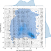 |
Fig. 1 Example of the uniform encoding grid of N2 rectangles (with N = 30) used to encode the planets over the logarithm of the mass and semi-major axis of the planets. For each rectangle, we attribute a unique Unicode character, in order to encode a planet lying inside. In blue the density distribution is shown for the population of the 25 000 planetary systems used to train the model. The levels correspond to fractions of 0.0001, 0.001, 0.01, 0.1, 0.2, 0.3, 0.4, 0.5, 0.6, 0.7, 0.8, 0.9, and 1. Note that if two planets (from the same system) are located in the same rectangle, they are encoded as two identical characters. |
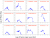 |
Fig. 2 Example of planetary systems belonging to our training database. The x-axis represents the log of the semi-major axis (in AU), the y-axis represents the log of the mass (in Earth masses). Each planetary system is represented as a broken line joining points, themselves representing planets. The characters in red in each of the panels correspond to the encoding of the planetary system into a word (see Sect. 3.1). |
Best cross entropy test loss obtained for different architectures of the generative model.
3.2 Transformer
Our model is based on the well-known transformer architecture, which leverages self-attention mechanisms (Vaswani et al. 2017). In this paper we do not describe all the details related to the transformer architecture. Instead, we point to the original paper by Vaswani et al. (2017). Our baseline model comprises only a decoder stack, which consists of three transformer layers, each using a single attention head. Contrary to language models, we did not use positional encoding, since the ‘position’ of a planet in the sequence encoding a planetary system is already hinted at by the character representing each planet1. The initial embedding for the different characters has a size of 32, while the final feed-forward neural network has one hidden layer with 128 units and uses the GeLU activation function (Hendrycks & Gimpel 2023). Our code was developed using PyTorch and closely follows the Makemore code of A. Karpathy2. The total number of parameters for the model is around 60 000.
3.3 Training
Our sample of 25 000 planetary systems was randomly split into a training set consisting of 24 000 samples and a test set consisting of 1000 samples. We trained our model using the AdamW optimiser of PyTorch3 with default parameters. We chose a learning rate of 5 × 10⁻⁴ and a weight decay of 0.01. The training was done over 70000 steps where the samples were processed in batches of 32. The entire training set was therefore processed, on average, every 730 steps.
For each sample/word, the model was trained to predict the next character accounting for the previous ones in the sequence. Each planetary system (or ‘word’) therefore contains many training sub-samples at once: to begin, we predicted the first character; then, we predicted the second given the first; then the third given the first two, and so on.
To evaluate the training phase, cross-entropy loss was used. This choice was justified by its popularity for multi-class classification problems and also because it provides a smooth and differentiable function for optimisation (Mao et al. 2023). In our case, the classes correspond to the different possible characters that can be attributed to a single planet.
The training took a few hours on a MacBook with an M2 Pro chip, and we achieved a best cross-entropy loss of 2.4014 after around 49 000 epochs (with one epoch corresponding to the evaluation of a batch of 32 samples). Table 1 shows the best test losses obtained for the different architectures, and Fig. 4 shows the evolution of the loss as a function of the training epoch for the best model. While decreasing and stagnating training and test loss over the training period are good indications that the model has learned the relationships between the different characters and how the words were formed, the loss value also provides insights into the success of the training. If a word were generated randomly from the different possible characters, a cross-entropy loss of log N, where N is the number of possible characters, would be expected. In our case, we can select from 440 different characters4, meaning that the cross-entropy loss for the worst generative model would be ~6.09. A cross-entropy loss of zero would indicate a perfect model, and a model with a loss around 2.40, as in our case, indicates a good model, capable of capturing the essence of the word generation, i.e. the planetary system’s architecture.
We also explored the effect of varying the parameters of our model, namely the dimension of the embedding, the number of blocks, the number of attention heads, and the inclusion of positional embedding (whose size is equal to the embedding). For all the tests, the number of units in the feed-forward network is equal to four times the embedding size. Table 1 shows that the value achieved for the best loss does not strongly vary for all the models we considered. For the rest of the paper, we only consider our nominal model.
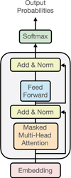 |
Fig. 3 Model architecture. The model is made of one embedding layer (dimension 16 to 128), two to eight blocks (grey rectangle) and one soft-max layer that predicts the probability of each character knowing all the previous ones. Each block is made of a masked multi-head attention layer (between one and eight heads), followed by a normalisation layer, a feed-forward neural network (one hidden layer, the number of units being four times the size of the embedding size), and a second normalisation layer. The different architectures tested (number of blocks, size of the embedding layer, and number of attention heads) as well as the best obtained cross-entropy loss are indicated in Table 1. |
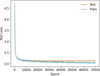 |
Fig. 4 Evolution of training and test cross-entropy loss as a function of the training epoch for the best generative model (see Table 1). |
4 Results
4.1 Visual comparison
We first examined the mass versus semi-major axis diagram of generated planetary systems to determine if they could be distinguished from those resulting from direct numerical simulations. Some examples are provided in Fig. 8. In some cases, the generated nature of an example can be inferred, while in others, it is difficult to determine from which population the sample is drawn.
4.2 Statistical comparison
Secondly, we conducted an initial comparison between the three populations: the original synthetic population (computed using the Bern model), a degraded synthetic population (using the Bern model, but applying an encoding followed by a decoding operation), and the generated population (computed with our generative model). In this case, the degraded synthetic population allows for a fair evaluation of the generative model alone, while comparing with the original population enables an evaluation of the entire process (including encoding-decoding) and an assessment of the total information loss. Fig. 5 shows the distributions of various quantities for the two populations. Some quantities are linked to the physical properties of planets (mass and semi-major axis), while others are linked to the representation of planetary systems as broken lines in a 2D plane. These quantities consist of:
the distribution of planetary masses (first row, left in Fig. 5);
the distribution of planetary semi-major axis (first row, middle);
the number of planets in the system (first row, right);
the (Euclidean) distance between two points representing two consecutive planets in the same system (second row, left); and
the angle between two segments of the broken line (second row, right).
As seen in Fig. 5, the statistical properties of the three populations are very similar in most cases. For the angle and length distributions, there is a mismatch around the smaller values, which is an artefact from the grid-based encoding and decoding method.
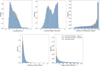 |
Fig. 5 Comparison between different properties of the populations considered. The numerical one is shown in orange; the degraded one (encoded and decoded to assess information loss) is shown in purple; and the one generated by the transformer is shown in blue. |
4.3 Machine learning-based comparison
Using our nominal model, we produced 25 000 generated systems. Together with the 25 000 synthetic systems, we randomly mixed the two populations, assigning the label one to the synthetic systems and the label zero to the generated ones. We then considered 18 different classifiers in order to classify the samples in the mixed population. For the classification problem, the 50 000 samples were split into 40 000 training samples, 5000 test samples, and 5000 validation samples. Our goal was to check whether the ML-based classification algorithms could distinguish between the two populations. We ran this exercise at different steps (each 100 epochs) during the training of our nominal model, as we expected that, very early in the training, it would be straightforward to distinguish between the numerical and generated populations. In contrast, in the ideal case – when the generative model is fully trained – it should become impossible to distinguish between the two populations.
Each of the classifiers, after training, produces a single value (between zero and one) that can be used to decide if a sample belongs to the numerical population or the generated one. For each classifier and each training step of our generative model, we computed the area under the curve (AUC) of the so-called receiver operating characteristic curve (ROC curve)5. A perfect classifier would have an AUC equal to 1, whereas in principle a value of 0.5 indicates a purely random choice. We used the Sci-kit library to compute the AUC6, and the classifiers were implemented using the Sci-kit (linear, support vector, and random forest) or Keras (feed forward deep neural networks) libraries7.
Table 2 summarises the different classifiers we considered, as well as some of their characteristics. We also quote, in this table, the AUC obtained by randomly splitting the numerical population equally into two parts, with one half being assigned the label zero, the other half the label one. In principle, since this is a homogeneous population, we expect that no classifier can solve this problem. We indeed see in the table that the AUC for each classifier is close to 0.5. We lastly quote the AUC obtained when classifying the numerical population versus the generated population computed using our generative model after training.
In Fig. 6, we plot the classification performances (quantified by the AUC) of a set of ML classifiers as a function of the training of the generative model. As expected, in the beginning, when there is little or no training of the generative model, all classifiers are able to distinguish between the numerical and generated populations (all values are close to one). As we train the generative model, it learns how to generate planetary systems properly (statistically similar to the training sample), and it becomes more and more difficult to distinguish generated systems from numerically computed ones. In this way, the performances of the classifiers decrease. At the end of the training, the AUC is very close to the values in Table 2, showing that no classifier can efficiently distinguish between the two populations. While it is possible that other classifiers could achieve better performance, this result gives us confidence that the statistical properties of the generated and numerical populations are very similar.
Classifiers considered for ML-based comparisons according to selected parameters.
Properties of planets b, c, and d from the TOI-469 system.
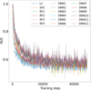 |
Fig. 6 AUC as a function of the training epoch of our generative model for different classification algorithms. |
5 Example
As a use case of our generative model, we considered the TOI-469 system (Damasso et al. 2023). This system, which has three observed planets, was first discovered by TESS with the detection of planet b and later observed using ESPRESSO, where two additional planets, c and d, were found. With additional observations (Egger et al. 2024), it was possible to characterise the properties of the three observed planets with high precision. Some of these properties are listed in Table 3.
We considered a scenario that could have followed shortly after the TESS discovery, when only TOI-469 b was known. We used our generative model to estimate the potential properties and number of planets in the system, accounting only for the properties of planet b. For this, we generated 300 000 planetary systems and selected the ones with a planet similar to TOI-469 b, allowing for a 10% uncertainty on the mass and 1% uncertainty on the semi-major axis. We assumed a minimum detectability threshold for the radial velocity (RV) semi-amplitude of K = 1.5 m/s and only considered planets that met this criterion for plotting. From the ~300 000 planetary systems, only around 350 have a TOI-469 b-like planet.
The final results can be seen in Fig. 7. The 2D histogram shows two concentrations of planets: one around the position of TOI-469 c and TOI-469 d, and one for the giant planets around 1 AU. Considering the distribution of the semi-major axis, planets c and d are located close to the main peak in the histogram. They are, on the other hand, slightly less massive than the peak of the mass histogram. According to our model, the number of planets with an RV semi-amplitude larger than the adopted cut-off ranges from two to four, and only 40% of the systems would have a giant planet (more massive than 100 M⊕ – such a planet would have been easily detected by ESPRESSO). We therefore conclude that the properties of systems compatible with those of TOI-469 b are consistent with the properties of the system characterised by ESPRESSO and CHEOPS.
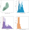 |
Fig. 7 Predictions, based on our generative model, of the properties of planets in systems that harbour one planet similar to TOI-469 b. Upper-left: 2D histogram in the log semi-major axis versus the log mass. The positions of planets c and d are indicated with a red cross, whereas the position of TOI-469 b is indicated by a white cross. Upper-right and lower-left: distribution of the log semi-major axis and the log mass, respectively. The positions of planets c and d are indicated by the red lines with a 10% uncertainty (light red region). Lower-right: distribution of the number of observable planets with K ≥ 0.15 m/s. |
6 Conclusions
We developed a model, which can be used to compute generated planetary systems. The model, based on the transformer architecture, was trained on a database of around 25 000 synthetic planetary systems computed using the ‘Bern model’ (Emsenhuber et al. 2021a,b), assuming a central star similar to the Sun. We only considered two features of synthetic planets (i.e. their total mass and their semi-major axis). We conclude that our generative model is able to produce generated planetary systems whose properties are statistically similar to those of the training database. This similarity was first checked visually8, then demonstrated by comparing different statistics of planetary systems, and further confirmed using machine-learning algorithms of different types.
Our model can be used to study fine statistics related to planetary system architecture, as well as to compute the probability distribution of some planet’s properties, given the observed properties of other planets in the same system. In a future step, we plan to develop this model to condition the generation of sequences on the main properties of the star and the protoplanetary disc in which the system was formed.
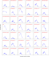 |
Fig. 8 Examples of planetary systems: half generated by our generative model, half from our training dataset. The x-axis represents the log of the semi-major axis (in AU); the y-axis represents the log of the mass (in Earth masses). Each planetary system is represented as a broken line connecting points, with each point representing a planet. The characters in red in each of the panels indicate the encoding of the planetary system (see Sect. 3.1). The exact populations, either generated or from numerical simulations, to which each system belongs is indicated in a footnote in our conclusions (Sect. 6). |
Data availability
The code is available at https://www.ai4exoplanets.com
Acknowledgements
The authors acknowledge support from the Swiss NCCR PlanetS and the Swiss National Science Foundation. This work has been carried out within the framework of the NCCR PlanetS supported by the Swiss National Science Foundation under grants 51NF40182901 and 51NF40205606. Part of this work has been developed in the framework of the Certificate for Advanced Studies ‘Advanced Machine Learning’ of the University of Bern. The authors thank the teachers and students of the CAS-AML.
References
- Basant, R., Dietrich, J., Apai, D., & Malhotra, R. 2022, AJ, 164, 12 [NASA ADS] [CrossRef] [Google Scholar]
- Beckwith, S. V. W., & Sargent, A. I. 1996, Nature, 383, 139 [NASA ADS] [CrossRef] [Google Scholar]
- Benz, W., Broeg, C., Fortier, A., et al. 2021, Exp. Astron., 51, 109 [Google Scholar]
- Brewer, J. M., Wang, S., Fischer, D. A., & Foreman-Mackey, D. 2018, ApJ, 867, L3 [NASA ADS] [CrossRef] [Google Scholar]
- Bryan, M. L., & Lee, E. J. 2024, ApJ, 968, L25 [NASA ADS] [CrossRef] [Google Scholar]
- Burn, R., Schlecker, M., Mordasini, C., et al. 2021, A&A, 656, A72 [NASA ADS] [CrossRef] [EDP Sciences] [Google Scholar]
- Chen, C., Martin, R. G., Lubow, S. H., & Nixon, C. J. 2024, AJ, 961, L5 [Google Scholar]
- Damasso, M., Rodrigues, J., Castro-González, A., et al. 2023, A&A, 679 [Google Scholar]
- Dannert, F. A., Ottiger, M., Quanz, S. P., et al. 2022, A&A, 664, A22 [NASA ADS] [CrossRef] [EDP Sciences] [Google Scholar]
- Davoult, J., Alibert, Y., & Mishra, L. 2024, A&A, 689, A309 [NASA ADS] [CrossRef] [EDP Sciences] [Google Scholar]
- Dietrich, J. 2024, AJ, 168, 119 [Google Scholar]
- Dietrich, J., & Apai, D. 2020a, AJ, 160, 107 [NASA ADS] [CrossRef] [Google Scholar]
- Dietrich, J., & Apai, D. 2020b, AJ, 161, 17 [Google Scholar]
- Dietrich, J., Apai, D., & Malhotra, R. 2022, AJ, 163, 88 [Google Scholar]
- Drążkowska, J., Bitsch, B., Lambrechts, M., et al. 2023, in Protostars and Planets VII, eds. S. Inutsuka, Y. Aikawa, T. Muto, K. Tomida, & M. Tamura, ASP Conference Series, 534, 717 [Google Scholar]
- Egger, J. A., Osborn, H. P., Kubyshkina, D., et al. 2024, A&A, 688 [Google Scholar]
- Emsenhuber, A., Mordasini, C., Burn, R., et al. 2021a, A&A, 656, A69 [NASA ADS] [CrossRef] [EDP Sciences] [Google Scholar]
- Emsenhuber, A., Mordasini, C., Burn, R., et al. 2021b, A&A, 656, A70 [NASA ADS] [CrossRef] [EDP Sciences] [Google Scholar]
- Emsenhuber, A., Mordasini, C., & Burn, R. 2023, Eur. Phys. J. Plus, 138, 181 [NASA ADS] [CrossRef] [Google Scholar]
- Fortier, A., Alibert, Y., Carron, F., Benz, W., & Dittkrist, K. M. 2013, A&A, 549, A44 [NASA ADS] [CrossRef] [EDP Sciences] [Google Scholar]
- Ghezzi, L., Martinez, C. F., Wilson, R. F., et al. 2021, ApJ, 920, 19 [Google Scholar]
- Gilbert, G. J., & Fabrycky, D. C. 2020, AJ, 159, 281 [Google Scholar]
- Haisch, Karl E., J., Lada, E. A., & Lada, C. J. 2001, AJ, 553, L153 [CrossRef] [Google Scholar]
- Hansen, J. T., Ireland, M. J., & LIFE Collaboration. 2022, A&A, 664, A52 [NASA ADS] [CrossRef] [EDP Sciences] [Google Scholar]
- He, M. Y., Ford, E. B., & Ragozzine, D. 2019, MNRAS, 490, 4575 [CrossRef] [Google Scholar]
- Hendrycks, D., & Gimpel, K. 2023, Gaussian Error Linear Units (GELUs) [Google Scholar]
- Ida, S., & Makino, J. 1993, Icarus, 106, 210 [NASA ADS] [CrossRef] [Google Scholar]
- Konrad, B. S., Alei, E., Quanz, S. P., et al. 2022, A&A, 664, A23 [NASA ADS] [CrossRef] [EDP Sciences] [Google Scholar]
- Latham, D. W., Rowe, J. F., Quinn, S. N., et al. 2011, ApJ, 732, L24 [NASA ADS] [CrossRef] [Google Scholar]
- Mao, A., Mohri, M., & Zhong, Y. 2023, Proc. Mach. Learn. Res., 202, 23803 [Google Scholar]
- Marchal, C., & Bozis, G. 1982, Celest. Mech., 26, 311 [Google Scholar]
- Millholland, S., Wang, S., & Laughlin, G. 2017, ApJ, 849, L33 [NASA ADS] [CrossRef] [Google Scholar]
- Mishra, L., Alibert, Y., Leleu, A., et al. 2021, A&A, 656, A74 [NASA ADS] [CrossRef] [EDP Sciences] [Google Scholar]
- Mishra, L., Alibert, Y., Udry, S., & Mordasini, C. 2023a, A&A, 670, A68 [NASA ADS] [CrossRef] [EDP Sciences] [Google Scholar]
- Mishra, L., Alibert, Y., Udry, S., & Mordasini, C. 2023b, A&A, 670, A69 [NASA ADS] [CrossRef] [EDP Sciences] [Google Scholar]
- Mordasini, C. 2018, in Handbook of Exoplanets, eds. H. J. Deeg, & J. A. Belmonte, 143 [Google Scholar]
- Murchikova, L., & Tremaine, S. 2020, AJ, 160, 160 [NASA ADS] [CrossRef] [Google Scholar]
- Murray, N., Chaboyer, B., Arras, P., Hansen, B., & Noyes, R. W. 2001, ApJ, 555, 801 [NASA ADS] [CrossRef] [Google Scholar]
- Ohtsuki, K., Stewart, G. R., & Ida, S. 2002, Icarus, 155, 436 [Google Scholar]
- Pepe, F., Cristiani, S., Rebolo, R., et al. 2021, A&A, 645, A96 [NASA ADS] [CrossRef] [EDP Sciences] [Google Scholar]
- Pollack, J. B., Hubickyj, O., Bodenheimer, P., et al. 1996, Icarus, 124, 62 [NASA ADS] [CrossRef] [Google Scholar]
- Quanz, S. P., Ottiger, M., Fontanet, E., et al. 2022, A&A, 664, A21 [NASA ADS] [CrossRef] [EDP Sciences] [Google Scholar]
- Sandford, E., Kipping, D., & Collins, M. 2021, MNRAS, 505, 2224 [NASA ADS] [CrossRef] [Google Scholar]
- Santos, N. C., Israelian, G., Mayor, M., Rebolo, R., & Udry, S. 2003, A&A, 398, 363 [NASA ADS] [CrossRef] [EDP Sciences] [Google Scholar]
- Schlecker, M., Mordasini, C., Emsenhuber, A., et al. 2021a, A&A, 656, A71 [NASA ADS] [CrossRef] [EDP Sciences] [Google Scholar]
- Schlecker, M., Pham, D., Burn, R., et al. 2021b, A&A, 656, A73 [NASA ADS] [CrossRef] [EDP Sciences] [Google Scholar]
- Steffen, J. H., Ragozzine, D., Fabrycky, D. C., et al. 2012, PNAS, 109, 7982 [NASA ADS] [CrossRef] [Google Scholar]
- Vaswani, A., Shazeer, N., Parmar, N., et al. 2017, Attention Is All You Need [Google Scholar]
- Veras, D., & Armitage, P. J. 2004, MNRAS, 347, 613 [Google Scholar]
- Weiss, L. M., Isaacson, H. T., Marcy, G. W., et al. 2018, AJ, 156, 254 [Google Scholar]
- Weiss, L. M., Millholland, S. C., Petigura, E. A., et al. 2023, in Protostars and Planets VII, eds. S. Inutsuka, Y. Aikawa, T. Muto, K. Tomida, & M. Tamura, ASP Conference Series, 534, 863 [Google Scholar]
- Winn, J. N., & Fabrycky, D. C. 2015, ARA&A, 53, 409 [Google Scholar]
- Zhu, W. 2020, AJ, 159, 188 [NASA ADS] [CrossRef] [Google Scholar]
- Zhu, W. 2024, Res. Astron. Astrophys., 24, 045013 [CrossRef] [Google Scholar]
- Zhu, W., & Wu, Y. 2018, AJ, 156, 92 [Google Scholar]
Note that we could have treated planetary systems as unordered sets instead of ordered sequences. Considering them as sequences is useful because, in this case, planet n + 1 is, by construction, at a larger semi-major axis than planet n. This implies that the conditional probability of planet n + 1 having a semi-major axis smaller than that of planet n is equal to zero. Such a property, which would not be true for a set, is learned by the transformer.
One would expect 900 classes from the N2 grid with N = 30. However, not all characters and/or rectangles of the grid appear in words and thus do not participate in the cross-entropy loss. Therefore, our classes are reduced to 440 instead.
This curve shows the true positive rate as a function of the false positive rate for all the values of the classification threshold (the threshold above which we decide that a sample belongs to the numerical population).
In Fig. 8, generated systems are located on columns 1, 3, and 5.
All Tables
Best cross entropy test loss obtained for different architectures of the generative model.
Classifiers considered for ML-based comparisons according to selected parameters.
All Figures
|
Fig. 1 Example of the uniform encoding grid of N2 rectangles (with N = 30) used to encode the planets over the logarithm of the mass and semi-major axis of the planets. For each rectangle, we attribute a unique Unicode character, in order to encode a planet lying inside. In blue the density distribution is shown for the population of the 25 000 planetary systems used to train the model. The levels correspond to fractions of 0.0001, 0.001, 0.01, 0.1, 0.2, 0.3, 0.4, 0.5, 0.6, 0.7, 0.8, 0.9, and 1. Note that if two planets (from the same system) are located in the same rectangle, they are encoded as two identical characters. |
| In the text | |
|
Fig. 2 Example of planetary systems belonging to our training database. The x-axis represents the log of the semi-major axis (in AU), the y-axis represents the log of the mass (in Earth masses). Each planetary system is represented as a broken line joining points, themselves representing planets. The characters in red in each of the panels correspond to the encoding of the planetary system into a word (see Sect. 3.1). |
| In the text | |
|
Fig. 3 Model architecture. The model is made of one embedding layer (dimension 16 to 128), two to eight blocks (grey rectangle) and one soft-max layer that predicts the probability of each character knowing all the previous ones. Each block is made of a masked multi-head attention layer (between one and eight heads), followed by a normalisation layer, a feed-forward neural network (one hidden layer, the number of units being four times the size of the embedding size), and a second normalisation layer. The different architectures tested (number of blocks, size of the embedding layer, and number of attention heads) as well as the best obtained cross-entropy loss are indicated in Table 1. |
| In the text | |
|
Fig. 4 Evolution of training and test cross-entropy loss as a function of the training epoch for the best generative model (see Table 1). |
| In the text | |
|
Fig. 5 Comparison between different properties of the populations considered. The numerical one is shown in orange; the degraded one (encoded and decoded to assess information loss) is shown in purple; and the one generated by the transformer is shown in blue. |
| In the text | |
|
Fig. 6 AUC as a function of the training epoch of our generative model for different classification algorithms. |
| In the text | |
|
Fig. 7 Predictions, based on our generative model, of the properties of planets in systems that harbour one planet similar to TOI-469 b. Upper-left: 2D histogram in the log semi-major axis versus the log mass. The positions of planets c and d are indicated with a red cross, whereas the position of TOI-469 b is indicated by a white cross. Upper-right and lower-left: distribution of the log semi-major axis and the log mass, respectively. The positions of planets c and d are indicated by the red lines with a 10% uncertainty (light red region). Lower-right: distribution of the number of observable planets with K ≥ 0.15 m/s. |
| In the text | |
|
Fig. 8 Examples of planetary systems: half generated by our generative model, half from our training dataset. The x-axis represents the log of the semi-major axis (in AU); the y-axis represents the log of the mass (in Earth masses). Each planetary system is represented as a broken line connecting points, with each point representing a planet. The characters in red in each of the panels indicate the encoding of the planetary system (see Sect. 3.1). The exact populations, either generated or from numerical simulations, to which each system belongs is indicated in a footnote in our conclusions (Sect. 6). |
| In the text | |
Current usage metrics show cumulative count of Article Views (full-text article views including HTML views, PDF and ePub downloads, according to the available data) and Abstracts Views on Vision4Press platform.
Data correspond to usage on the plateform after 2015. The current usage metrics is available 48-96 hours after online publication and is updated daily on week days.
Initial download of the metrics may take a while.