| Issue |
A&A
Volume 701, September 2025
|
|
|---|---|---|
| Article Number | A203 | |
| Number of page(s) | 12 | |
| Section | Interstellar and circumstellar matter | |
| DOI | https://doi.org/10.1051/0004-6361/202453498 | |
| Published online | 17 September 2025 | |
Multi-scale radiative-transfer model of the protoplanetary disc DoAr 44
1
Charles University, Faculty of Mathematics and Physics, Astronomical Institute,
V Holešovičkách 2,
18000
Prague,
Czech Republic
2
Heidelberg University, Department of Physics and Astronomy,
Im Neuenheimer Feld 226,
69120
Heidelberg,
Germany
★ Corresponding author: This email address is being protected from spambots. You need JavaScript enabled to view it.
Received:
18
December
2024
Accepted:
18
July
2025
Abstract
Aims. Our aim was to construct a comprehensive global multi-scale kinematic equilibrium radiative-transfer model for the pretransitional disc of DoAr 44 (Haro 1-16, V2062 Oph) in the Ophiuchus star-forming region. This model integrates diverse observational datasets to describe the system, spanning from the accretion region to the outer disc.
Methods. Our analysis utilised a large set of observational data, including ALMA continuum complex visibilities, VLTI/GRAVITY continuum squared visibilities, closure phases, and triple products, as well as VLT/UVES and VLT/X-shooter Hα spectra. Additionally, we incorporated absolute flux measurements from ground-based optical observatories, Spitzer, IRAS, the Submillimeter Array, the IRAM, or the ATCA radio telescopes. These datasets were used to constrain the structure and kinematics of the object through radiative-transfer modelling.
Results. Our model reveals that the spectral line profiles are best explained by an optically thin spherical inflow or outflow within the co-rotation radius of the star, exhibiting velocities exceeding 380 km/s. The VLTI near-infrared interferometric observations are consistent with an inner disc extending from 0.1 to 0.2 au. The ALMA sub-millimetre observations indicate a dust ring located between 36 and 56 au, probably related to the CO2 condensation line. The global density and temperature profiles derived from our model provide insight into an intermediate disc, located in the terrestrial planet-forming zone, which has not yet been spatially resolved.
Key words: accretion, accretion disks / radiative transfer / techniques: interferometric / protoplanetary disks / submillimeter: planetary systems
© The Authors 2025
 Open Access article, published by EDP Sciences, under the terms of the Creative Commons Attribution License (https://creativecommons.org/licenses/by/4.0), which permits unrestricted use, distribution, and reproduction in any medium, provided the original work is properly cited.
This article is published in open access under the Subscribe to Open model. This email address is being protected from spambots. You need JavaScript enabled to view it. to support open access publication.
1 Introduction
Protoplanetary discs are reservoirs of gas and dust surrounding young stellar objects and are the birthplaces of planets. Understanding them is necessary to understand the formation of exoplanetary systems and our own Solar System. Various disc morphologies have been suggested based on the broadband spectral energy distribution, and now are being directly imaged either via sub-millimetre observations or adaptive optics (Andrews et al. 2018; Avenhaus et al. 2018). Presumably, the youngest of these discs have monotonically decreasing density profiles, with a large inner cavity opening later (most probably due to the influence of forming ice giants) thus creating what are called transitional discs (van der Marel 2023), before dispersing a few million years later (Li & Xiao 2016). However, matter is still flowing through these cavities, as evidenced by the high accretion rates (van der Marel 2023).
An intermediate phase has been identified (Espaillat et al. 2007), called the pre-transitional phase, where the young star is surrounded by an inner disc and is encircled by a large optically thin cavity, followed by an extended dust ring exhibiting millimetre-emission.
The object DoAr 44 (Haro 1-16, V2062 Oph), located in the Ophiuchus star formation region, is one of these pre-transitional discs with a high water vapour luminosity in the inner disc (Salyk et al. 2015), 40 times more luminous in the 17 μm water line than the structurally very similar disc PDS 70 (Perotti et al. 2023), where planet formation is confirmed by direct imaging by the Hubble Space Telescope (HST) (Zhou et al. 2021), ALMA (Benisty et al. 2021) and VLT/SPHERE (Keppler et al. 2018). DoAr 44 has been investigated by VLTI/GRAVITY (Bouvier et al. 2020b), revealing a disc-like structure in the 0.2–1.5 au region and by VLT/SPHERE (Arce-Tord et al. 2023). These investigations show the disc extending beyond 15 au and also ALMA Bands 3, 4, 6, 7, and 8 at resolutions up to ≈25 mas in Band 6 and 7 (Cieza et al. 2021; Arce-Tord et al. 2023), in both continuum and spectral lines, investigating the region from 5-80 au, revealing a narrow dust ring with a brim around 47 au.
A series of other works were devoted to this pre-transitional disc. For example, Ricci et al. (2010a) performed a 3.3 mm continuum survey of the \varrho Ophiuchi region, including DoAr 44, using the Australian Telescope Compact Array (ATCA), measuring the spectral indices between the 1.3 mm and 3.3 mm fluxes. They concluded that the spectral indices of Ophiuchus sources are not statistically different from the sources in the Taurus-Auriga star-forming region, which they surveyed using the Plateau de Bure Interferometer (PdBI) in a previous study (Ricci et al. 2010b), but differ significantly from the interstellar medium.
Andrews et al. (2010) then performed an interferometric survey using the Submillimeter Array (SMA) at 40 au resolution in the Ophiuchus star-forming region. They tried fitting the surface density profile using the common Lynden-Bell & Pringle (1974) prescription
![Mathematical equation: $\Sigma=\Sigma_{0}\left(\frac{R}{R_{c}}\right)^{\gamma} \exp \left[-\left(\frac{R}{R_{c}}\right)^{2-\gamma}\right],$](/articles/aa/full_html/2025/09/aa53498-24/aa53498-24-eq1.png) (1)
(1)
where Σ0, Rc, γ are parameters. However, for several discs they found a poor fit, which could be explained by the fact that these discs (DoAr 44, SR 21, SR 24, and WSB 60) had a large central cavity. This was the first spatially resolved observation of the cavities predicted by SED modelling. They continued their investigation of transitional discs with an additional SMA study (Andrews et al. 2011), finding that the dust in the cavity has been depleted by 4-6 orders of magnitude with respect to the Lynden-Bell & Pringle (1974) profile.
Espaillat et al. (2010) modelled Infrared Telescope Facility (IRTF) 2.1-5.0 micron spectra of DoAr 44 with R=1500 resolving power, and also Spitzer spectra, using analytical temperature prescriptions. They derived a higher accretion rate of  .
.
Bouvier et al. (2020b) obtained K-band (2–2.4 μm) continuum and Brγ line visibilites of DoAr 44 from VLTI/GRAVITY. They concluded that the Brγ emission is located inward of the continuum emission, suggesting that the optically thin gas flows, where the line emission is created, are located within the truncation radius. They used the Lazareff et al. (2017) visibility models, using a point source, an elliptical Gaussian in place of the disc and a halo. This halo represents all the incoherent emission from outside regions. They found the contribution of the ellipse to be 27%, the star 67%, and the halo 6%.
Bouvier et al. (2020a) also performed multi-colour photometry from the Las Cumbres Observatory Global Telescope Network (LCOGT) and spectroscopy using the Canada-France-Hawaii Telescope (CFHT). They found a rotation period of P = 2.96 days, and a stellar inclination of i = (30 ± 5)°, which is in agreement with the inclination of the ellipse modelling what is supposedly the inner rim seen by VLTI. From their Hα, Hβ, Paβ, and Brγ spectra, they conclude that the spectral line profiles are best explained as a combination of funnel flows along magnetic field lines and disc winds, similar to the ones described by radiative transfer models by Kurosawa et al. (2011), where the funnel flows cross the line of sight. For some spectral lines, this behaviour is periodic (He I), and for others, a more complicated chaotic variability (Brγ) is reported. Bouvier et al. (2020a) derived an accretion rate of  .
.
Avenhaus et al. (2018) studied discs around T Tauri stars (the DARTTS-S survey), using the VLT/SPHERE/IRDIS instrument, operating in the range of 0.9–2.3 microns, in the differential polarimetric imaging mode, with a coronagraph obscuring 0.1′′ around the central star. These images can be seen in Figs. A.3A and A.3B; they show the scattered light from the surface of the disc. Surprisingly, they found no correlation of the scattered light, either to the stellar mass or to millimetre fluxes.
Casassus et al. (2018) focused on the misalignment of the inner and outer discs of DoAr 44. This is somewhat visible in the radio continuum, but it is very apparent in the polarimetric images. They estimated a tilt of 30° of the inner disc with respect to the outer disc using radiative transfer modelling.
Casassus et al. (2019) constructed a parametric radiative transfer model of DoAr 44, which accounted for the shadowing caused by the misaligned inner disc. They derived outer disc dust temperatures of 36–48 K with the cooler temperatures being in the nodal regions shadowed by the inner disc. They derived a surface density of Σ= < 13 cm2 g−1 and an aspect ratio of 0.08 at the inner rim of the outer ring.
Parameters of the VLT observations of the Hα spectrum of DoAr 44.
Arce-Tord et al. (2023) studied these same SPHERE images together with the ALMA Band 6 images from ODISEA and new Band 7 images, specifically of the DoAr 44 system. They derived a relative inclination of 21°.
Leiendecker et al. (2022) performed a study of DoAr44, together with the better known system HD 163296. They estimated a dust mass of 0.3 MJupiter, corresponding to 21.5 MJupiter mass of gas. They tried explaining the ring morphology in alternative scenarios, such as a break-up of two large bodies. They also estimated the mass of a hypothetical planet needed to clear the inner disc at 0.5 to 1.6 MJupiter. For this work, our aim is to construct a global model of the system DoAr 44 informed by a wide range of observables.
2 Archival observations
Several archival observations of DoAr 44 are available, including Hα spectra, VLTI interferometry, ALMA visibilities, and spectral energy distribution measurements.
2.1 Hα spectroscopy
To constrain the physical properties of the accretion region around the star, all available Hα datasets from the ESO Archive were utilised. This includes 11 spectra from the VLT/ESPRESSO (programme ID 111.250 K), 3 spectra from VLT/UVES (programme ID 69.C-0481), and a single spectrum taken by VLT/X-shooter (programme ID 085.C-0764).
The VLT/ESPRESSO observations have a 2600 s exposition time and have a spectral resolution of R = 140 000. The signal-to-noise ratio (S/N) in the continuum around Hα is better than S/N ≳ 50, and reach S/N ≈ 200 in the centre of the spectral line profile. Further details can be found in Table 1.
The Hα emission is extremely variable, changing from 6 to 12 times above the continuum emission, displaying single-, double-, triple-, and even quadruple-peaked profiles. This behaviour is extremely complicated, and is related to the detailed geometry and kinematics of the accretion funnel flows and accretion shocks, and the superposition of emission and absorption components (Bouvier et al. 2020a).
For this reason, a mean profile was computed (see Fig. 1), corresponding approximately to an axially symmetric mean state of the system.
A piece-wise linear interpolation was performed in 200 equidistant points in the range 654.5–658.0 nm for all the datasets, and a point-wise average and standard deviation from this average was computed. This standard deviation from the mean spectrum was treated as the denominator in the χ2 minimisation, as our model does not capture the temporal variability of the system.
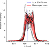 |
Fig. 1 Individual VLT Hα spectra of DoAr 44 and a mean spectrum. The spectrum is temporally variable, so a mean spectrum is used to constrain the mean state of the system. |
2.2 VLTI interferometry
To constrain the spatial extent of the inner accretion region, we utilised archival VLTI/GRAVITY interferometric data of DoAr 44 (Bouvier et al. 2020b). The reduction was performed using the Gravity Pipeline in EsoReflex (Freudling et al. 2013) in order to obtain the calibrated squared visibilities V2 and closure phases arg T3. The data was taken on 22 June 2020 using the Unit Telescopes in the K-band (≈ 2 μm). The uv-space coverage, together with the squared visibilities are shown in Fig. 2.
2.3 ALMA interferometry
To constrain the dimensions and temperature of the outer disc, the newest continuum Band 7(870 μm) ALMA interferometric data was used (project code 2019.1.00532.S, observation date 2021-08-19, Arce-Tord et al. (2023)). The minimum and maximum recoverable scales of the observations are 0.023 “and 0.56”, respectively, with a total 4390 s of integration time. The squared visibilities for both polarisations are shown in Fig. 3. The CLEANed image can be seen in A.3.H.
A second high-resolution observation in ALMA Band 6 (project code 2018.1.00028.S, observation date 2020-11-30, Cieza et al. (2021)) was also taken in consideration when modelling the intermediary disc. This observation can be seen in A.3.G. Other ALMA observations, which are listed in Table 2, have been used as total flux measurements, that is, as data points in the SED.
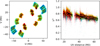 |
Fig. 2 VLTI/GRAVITY K-band interferometric visibilities of DoAr 44. Left: UV coverage of the observations in M λ. Right: squared visibility as a function of UV distance ( |

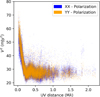 |
Fig. 3 ALMA Band 7 Squared visibilites of DoAr 44 for both polarisations (XX, YY) plotted separately as a function of uv-distance in Mλ. |
2.4 Spectral energy distribution
The measurements of the SED were taken from the following surveys, publications, and catalogues, using mostly Vizier (Ochsenbein et al. 2000):
XMM-Newton, 344 nm (Page et al. 2012);
ASAS-SN catalogue, 444 nm–2.16 μm (Jayasinghe et al. 2018);
SkyMapper catalogue, 497 nm, 604 nm (Bessell et al. 2011);
Gaia satellite, 505 nm, 673 nm (Gaia Collaboration 2018, 2020);
AAVSO Photometric All Sky Survey (APASS), 482 nm – 763 nm (Henden et al. 2016);
Sloan Digital Sky Survey (SDSS), 482 nm, 763 nm (York et al. 2000);
Pan-STARRS survey, 613 nm – 960 nm (Kaiser et al. 2002);
2MASS, 1.65 μm, 2.16 μm (Skrutskie et al. 2006);
Wide-field Infrared Survey Explorer (WISE), 3.35 μm, 11.6 μm (Wright et al. 2010);
Spitzer/IRAC, 3.6 μm–7.8 μm (Fazio et al. 2004);
Spitzer/MIPS, 70 μm (Rieke et al. 2004);
IRAS satellite, 11.6 μm, 61 μm (Neugebauer et al. 1984);
AKARI satellite, 18 μm, 90 μm (Takita et al. 2010);
Herschel/PACS, 100 μm, 160 μm (Billot et al. 2006);
Herschel/SPIRE, 250 μm, 350 μm (Griffin et al. 2010);
JCMT, 850 μm (Mohanty et al. 2013);
ATCA, 3 mm (Ricci et al. 2010a).
Currently available ALMA observations of DoAr 44.
Moreover, the integrated ALMA photometry was used, together with the interferometric observations described below. The X-ray data from Montmerle et al. (1983) were not used as the X-ray emission is formed under non-LTE conditions, which is outside the approximations of our models.
3 Simple analytic models
Before we begin constructing radiative-transfer models, it is useful to construct a few simple analytic models to act as benchmarks for our later work. With these analytic models approximately describe the observed interferometric visibilities. These models are as follows:
A homogeneous ellipse described by α, β, ω, together with a point source and a background halo for the VLTI/GRAVITY visibilities, to model the inner disc.
A narrow elliptical ring with a background halo for the ALMA visibilities, to model the outer disc.
Similar models were used by Lazareff et al. (2017) to model VLTI/PIONIER visibilities of about 50 Herbig AeBe discs. The introduction of a halo allows us to lower the visibility at short baselines that are not sampled by the VLTI. However, this contribution is not merely a mathematical aid, but is directly observed by coronagraphic instruments, such as the VLT/SPHERE (see Figure A.3). The two models can be described as follows:
 (2)
(2)
 (3)
(3)
Here the visibility of an ellipse, describing the circumstellar disc, is
 (4)
(4)
and of a δ-ring is
 (5)
(5)
Best-fit parameters of the homogeneous ellipse model suitable for the VLTI measurements of the accretion region.
Best-fit parameters of the elliptical δ-ring model, suitable for the ALMA visibilities.
with the rotated aperture-plane coordinates given by
 (6)
(6)
The parameters fc, fh, fs denote the fractional contributions of the circumstellar disc, the halo, and the star. The coordinates u, v and the angular sizes α and β are dimensionless, that is, given in cycles per baseline and in radians, respectively. As the separations of the telescopes (or antennas) is much larger than the wavelength that we are observing, we commonly use dimensionless units such as Mλ to denote 106 cycles per baseline. The best-fit parameters are estimated in Tables 3 and 4.
These analytic models were used as a benchmark for the more complex radiative-transfer models, providing the angular extent of the observed structures as a guide. They also provided a way to deal with the fully resolved component in the VLTI observations, and with the ALMA observations, which are in physical units and not in relative units. The interferometric quantities were rescaled in the following way:
 (7)
(7)
 (8)
(8)
 (9)
(9)
Here e=0.928 from the homogeneous ellipse model, and A, B are taken from the elliptical δ-ring model. The best-fit parameters and their uncertainties (68% confidence intervals of the marginalised posterior distributions) were obtained via a MCMC simulation with an uninformative prior. In each case, two solutions were obtained for two position angles separated by 180°, and only the solution with ω < 180° was considered. Initial simulations were performed with 32 walkers and 104 steps. The marginalised posteriors were used as a starting value for the next iteration: these new simulations ran with 64 walkers for a total of 105 steps, with a 30% burn-in phase. All simulations were implemented using the emcee package (Foreman-Mackey et al. 2013). From all these models, we infer an inclination of the inner accretion region at iin=40° ± 3° and of the outer disc at iout=22° ± 1°. The positions angles seem to be somewhat aligned, at ωin=147° ± 2° for the inner accretion region and ωout=156° ± 2° for the outer disc. The misalignment ξ can be calculated, for example, using the spherical law of cosines:

For comparison, Bohn et al. (2022) investigated the inner and outer disc misalignment of a series of protoplanetary discs, including DoAr 44, also based on VLTI/GRAVITY and ALMA interferometry. For DoAr 44, they derived an inner disc inclination of  and an outer disc inclination of
  .
.
Casassus et al. (2018) used VLT/SPHERE/IRDIS polarimetric measurements and ALMA Band 7 continuum measurements to derive a misalignment of ξ=30° ± 5°. Bouvier et al. (2020b) derived an inner disc inclination of iin=34° ± 2° based on VLTI/GRAVITY interferometric visibilities, with a position angle of ωin=140° ± 3°. Arce-Tord et al. (2023) derived outer disc inclinations for two high-resolution ALMA Band 6 and Band 7 observations, iout=21.8° ± 0.3°. Alternatively, they derived an outer disc inclination of 24.4° ± 0.4° using H-band polarised intensity images from VLT/SPHERE/IRDIS. They derived an inner-outer misalignment of  .
.
In conclusion, our results are in agreement for the outer inclination (1 σ), and for the new value of misalignment. The inner inclination is more uncertain, as the differences between models seem to be of the order of 2 σ.
4 Pyshellspec radiative-transfer models
The primary tool used to create radiative transfer models for this work, Pyshellspec, was developed by Mourard et al. (2018) and Brož et al. (2021) to model the β Lyræ A system. Pyshellspec generates various observables, such as interferometric visibilities and closure phases, based on synthetic images generated by Shellspec, a long-characteristic radiative-transfer code by Budaj & Richards (2004). Shellspec is used for modelling binary stars moving within circumstellar matter (i.e. gas and dust), and includes a series of parametrically defined objects, such as stars, rings, discs, jets, or spherical shells, which are described below.
The radiative-transfer equation is integrated along the line of sight,
 (10)
(10)
where ϵv, χv are the total emissivity and the total opacity of the medium, Iv is the specific monochromatic intensity, and dx is measured along the ray.
The total opacity is given as the sum of the absorption opacity κv and the scattering opacity σv:
 (11)
(11)
Shellspec allows the user to include the following sources of absorption opacity in κν:
Spectral line opacity,
HI (neutral hydrogen) bound-free opacity,
HI free-free opacity,
H− (negative hydrogen ion) bound-free opacity,
H− free-free opacity,
Mie absorption on dust,
and the following sources of scattering opacity:
Thompson (i.e. low-energy Compton) scattering on free electrons,
Rayleigh scattering on neutral hydrogen,
Mie scattering on dust.
The dust opacities are summed over all the included dust species that are located in a cold enough region, allowing for dust condensation.
The total emissivity is calculated as the sum of the thermal emissivity and the emission due to scattering,
 (12)
(12)
where Bv is the Planck function. One limitation is that Pyshellspec is a single-scattering radiative-transfer tool. This means that the stellar light scattered off the disc is accounted for in the synthetic image. We tested models with and without scattering opacity. The absorptive term leads to a decrease in the SED at mid-infrared wavelengths; however, this should be at least partly compensated for by the emissive term, scattering thermal radiation from other directions, if it is accounted for and if the intensity is approximately isotropic. According to these tests, we consider our nominal models as good approximations.
For the evaluation of the goodness of fit, a standard χ2 metric is defined,
 (13)
(13)
where  is the χ2 contribution from the spectroscopic data,
  the squared visibilities,
  the closure phases,
  the triple product amplitudes, and
  the SED. These are defined as
 (14)
(14)
 (15)
(15)
 (16)
(16)
 (17)
(17)
 (18)
(18)
where Iλ, obs and Iλ, syn respectively denote the observed and synthetic monochromatic intensities, V the visibilities, arg T3 the closure phases, |T3| the triple product amplitudes, and Fλ the monochromatic fluxes.
However, the total χ2 was not optimised globally as this is exceedingly difficult. The only contribution optimised globally was  , while the other contributions were optimised separately for the accretion region, the inner disc, and the outer disc.
Our model comprises three main parts:
the accretion region, described in our model using a star, a shell of infalling gas, and a hot innermost disc (up to 0.1 au);
an intermediary disc (0.2-1 au);
the outer disc (40-60 au).
The discs and the spherical shell were modelled using Shellspec’s DISC and SHELL objects, respectively.
4.1 The central star
The simplest element in our model is the central star. A synthetic stellar spectrum is provided as a boundary condition. This stellar spectrum was obtained by interpolation in the PHOENIX grid (Husser et al. 2013), similarly to that in Nemravová et al. (2016). The interpolation was performed in the three-dimensional parameter space of the effective temperature Teff, the (logarithm of) surface gravity log g, and the metallicity Z. The stellar parameters were set according to previously published works (Andrews et al. 2009; Bouvier et al. 2020b), r*=2.0 R⊙, T*=4750 K, M*=1.4 M⊙.
4.2 The DISC object
The primary object used to model discs in shellspec is the DISC. The disc is parametrised by the following equations:
 (19)
(19)
 (20)
(20)
 (21)
(21)
 (22)
(22)
 (23)
(23)
The following parameters are used:
Σ(Rinnb), Rinnb, and edensnb describe the surface density, inner radius, and density power-law exponent, respectively;
H(R) represents the disc’s scale height;
v(R) denotes the Keplerian velocity;
cs is the speed of sound, with γ=cp/cv (the ratio of specific heats) and μ (the mean molecular weight);
T(R) describes the temperature profile, parametrised by Tnb (the temperature normalisation) and etempnb (the temperature exponent);
ϱdstnb represents the dust density in the protoplanetary disc, linked to the gas density ϱnb through a constant (solar) metallicity Z=0.0122 (Asplund et al. 2006).
The model accounts for scattering and absorption opacities due to dust particles of various sizes and mineral compositions. A mix of 90% water ice and 10% forsterite is used as a proxy for the actual mineralogical composition. This is a slightly higher ratio than the traditional 80% ices to 20% refractory materials (Dodson-Robinson & Salyk 2011; Pontoppidan et al. 2014). Detailed dust evolution modelling suggests that virtually all dust grains in the outer disc are covered in ice (Krijt et al. 2016), thus impacting its optical properties (Köhler et al. 2015; Ysard et al. 2018). We account for this fact using an increased water ice content.
4.3 The SHELL object
The velocity v(r), density, and temperature profiles in the SHELL are described as
 (24)
(24)
 (25)
(25)
 (26)
(26)
where rcsh, rinsh, edenssh are parameters. The shell is truncated at an outer radius routsh. To obtain a contribution to the opacity due to Thompson scattering, the electron number density is computed using the Saha equation based on the local densities and the temperature, with the assumption of LTE.
4.4 Accretion region model
The geometry that best replicates the observables is a central star, surrounded by a spherical shell of hot gas, surrounded by a disc. The geometry of the disc was taken from the MCMC analysis of the analytic models; the inclination of i=40° is fixed, together with the position angle of 147°. The comparison of the spectroscopic and interferometric VLT+VLTI measurements with our synthetic data is shown in Figure 4.
A search for the best fit was performed on a sub-space of the parameter space that was identified (via trial and error) as being spanned by the most relevant parameters:
Routsh, the outer radius;
v(Rinsh), the velocity at the inner boundary;
evelsh, the exponent of the power law describing the velocity field of the shell;
Tsh, the (constant) temperature;
ϱsh, the density at the inner boundary.
The value of Rinsh had to be fixed slightly above the stellar surface (to avoid a collision with the STAR object).
The central star dominates the flux contribution in the optical domain. The star is surrounded by an envelope of optically thin hot (≈ 9000 K) gas, with a density of (≈ 2 × 10⁻¹³ g cm−3). This envelope extends up to about 0.1 au, where it encounters the innermost disc, and is responsible for the majority of the Hα emission. The radial velocity of the gas in this envelope reaches v=385 km s−1 The inner rim of this disc is the main source of near-infrared continuum radiation, and is responsible for the observed VLTI/Gravity visibilities.
The model was fitted to the VLTI/Gravity observations, the VLT H α spectra. The respective normalised χ2 contributions are  and
and  . The best-fit values of these parameters are listed in Table 5. From the density and velocity of the gas in the accretion envelope shell, we derive an accretion rate of
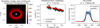 |
Fig. 4 Left: Synthetic image of the accretion region, in the 2 μm continuum. Centre: fit of VLTI/GRAVITY squared visibilities. Right: fit of the averaged Hα profile. The blue region is the standard deviation of the VLT spectra, representing the temporal variability. |
 (27)
(27)
which is surprisingly similar to the result obtained by Bouvier et al. (2020a). As the temperatures and spatial scales of this accretion region clearly do not account for the SED at millimetre wavelengths and ALMA visibilities, we must model the cold outer disc.
4.5 Outer disc model
To account for the ALMA visibilities and CLEANed images, we were forced to introduce a cavity (see Fig. 5). A scan over a variety of parameters (particle size, temperature, density, inner radius, outer radius) fitting the  was performed. The constraint on the total area of the disc is given primarily from the ALMA interferometry, where the inner and outer boundaries are visible (up to the background RMS level, the dust extends up to ≈ 80 au, see Fig. A.3). The density profile was simplified to a power law, and the complex ring-within-a-ring morphology was not fitted in detail.
In our model, the outer disc extends from 40 au to 60 au, with the mid-plane dust density of 1 × 10⁻¹⁴ g cm−3 at the inner boundary. The dust is given by a mix of water ice and forsterite, in a ratio of 90% and 10%, with particle sizes of a=1 μm. The mid-plane temperature at the 40 au inner boundary is 60 K, and decreases as a power law with an exponent of −0.5.
The aspect ratio H/r is 0.08 for the inner region of the outer disc (40 au), in agreement with Casassus et al. (2018), which then gradually increases to 0.10 in the outermost regions (60 au). By integrating the vertical density profile, we obtain the dust surface density of the order of Σdust ≳ 0.5 g cm−2. By integrating over the radial direction, we obtain the dust mass of
 (28)
(28)
However, this is still a lower limit as the outer disc in our model is optically thick: the best-fit dust density estimations do not have a clear upper limit from fitting the SED as various optically thick solutions appear very similar (see Fig. 6).
For comparison, Cieza et al. (2021) assumed a single value of temperature of T=20 K and derived Mdust=54 MEarth for DoAr 44, which is again a lower limit. Our model requires an optically thick outer disc in the 870 μm continuum, which is necessary to explain the SED and the sub-millimetre spectral index of α ≈ 2. The work Arce-Tord et al. (2023) also suggests that the disc is optically thick, based on the well-constrained spectral index.
Leiendecker et al. (2022) derived a dust mass of  for the outer disc, based on ALMA Band 6 observations. Their mid-plane temperatures are around 30 K, and they increase with increasing height above the mid-plane. On the contrary, our model is vertically isothermal, and requires about 50–60 K in the outer regions, in order to account for the Spitzer/MIPS (70 μm) and Herschel/PACS (100 μm) far-infrared fluxes.
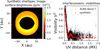 |
Fig. 5 Left: synthetic image in the 870 μm continuum of the best-fit model of the outer disc of DoAr44. Right: fit of the ALMA Band 7 squared visibilities. |
4.6 Intermediate disc model
A model consisting of the innermost region and the outer disc is enough to account for the spectra, the interferometric observables, and the SED measurements in the visible to near-IR, as well as the sub-millimetre and millimetre regions. However, a deficit in the SED is present in the mid-IR, which has to be compensated for by introducing a warm intermediary region in the 0.2-1 au range (see Fig. 7). We modelled this region using a DISC object, and its parameters can be found in Table 5. The global density and temperature profiles can also be found in Table 5.
The temperature at the inner edge reaches 1000 K, and drops to 380 K at the outer edge. Salyk et al. (2015) detected a large water-vapour luminosity originating from DoAr 44 using the Gemini-North telescope, and deduced the temperature of this water vapour to T ≈ 450 K. In our model these temperatures are reached precisely in this intermediate disc.
It appears that this intermediate disc region has been imaged, but unresolved, by the ODISEA programme in Band 6 (Cieza et al. 2021) (see Fig. A.3.H). However, the dimensions of this intermediate disc are not constrained by interferometry or other spatially resolved methods. This means that there exists a large set of acceptable models of this region, extending up to 5–7 au.
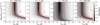 |
Fig. 6
|

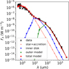 |
Fig. 7 SED measurements of DoAr 44 and a synthetic SED, made up of several components. The central star and accretion region dominate in the ultraviolet and visible range, and the outer disc is dominant in the sub-millimetre and millimetre wavelengths. These two contributions are well constrained from VLTI and ALMA interferometry. However, if only these two components are considered, a large deficit is present in the mid-infrared range. Therefore, an intermediate region must be present. The error bars are not visible, as the vertical axis spans ten magnitudes. |
5 Discussion
We now discuss the broader implications of our global model of DoAr 44 for the disc geometry, condensation of solids, and planet formation.
Best-fit parameters of the global model.
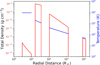 |
Fig. 8 Total (gas + dust) density and temperature profiles of DoAr44, with the assumed metallicity of Z=0.0122. The model is composed of four segments (from left to right): 1. A hot optically thin shell where Hα emission originates; 2. An innermost disc, which presumably feeds the accretion shell; 3. An intermediate disc, necessary to explain the SED in the mid-IR region; 4. A cold outer disc, visible with the ALMA. Between the intermediate and the outer disc, a large ≈ 30 au cavity is present. |
5.1 The geometry of the accretion region
As discussed in Sect. 2.1, the detailed geometry of the inner accretion region is variable on the scale of days, and is most likely connected to magnetic funnel flows, described in Bessolaz et al. (2008); Takasao et al. (2018); Bouvier et al. (2020a). We modelled the inner optically thin matter responsible for the averaged Hα emission using axially symmetric conical shapes, but optimising always resulted in large opening angles, or a spherically symmetric shell of gas.
Around this optically thin shell of gas, we included an optically thick innermost disc to explain the VLTI/GRAVITY visibilities. In our model, the innermost disc appears to be misaligned by about (18.5 ± 4)° with respect to the outer disc. The topic of misaligned protoplanetary discs has gained significant attention in recent years as these discs could produce exoplanets on highly inclined orbits, which are now readily observed using the Rossiter-McLaughlin effect (Zak et al. 2024).
A variety of mechanisms to produce a misaligned disc have been identified, for example compact stellar binaries (Nixon et al. 2013), or using an outside perturbing companion Doğan et al. (2015), stellar fly-bys (Nealon et al. 2019), or oblique infall (Kuffmeier et al. 2021). In our case, we can rule out the presence of a compact binary within the inner disc from the VLTI/GRAVITY observations, no infall is currently observed with ALMA, and no planetary companions have been confirmed, so the origin of this misalignment remains uncertain.
5.2 Causes of the ring: volatile or exoplanet
The overall temperature profile in our model predicts ∼50–60 K around the distance of 48 au in order to account for far-infrared continuum radiation. This relatively high temperature of layers emitting the respective radiation, compared to Leiendecker et al. (2022), among others, prevents the condensation of certain solids (Martín-Doménech et al. 2014).
The scientific literature on Solar System comets, which originate from these cold outer regions, is a good guide with respect to the expected chemical composition. The major volatiles found in comets are H2O, CO, CO2, CH4, and NH3, with water ice being typically the most abundant (Mumma & Charnley 2011). The comet’s composition is often given with respect to the water ice content. CO can contribute up to 30% of the mass of the water ice, CO2 up to 10%, and the other chemicals generally less than 1% (Greenberg 1998). Different ratios were obtained for example by Rosetta orbiting 67P/Churyumov-Gerasimenko, where CO2 formed 7.5% and CO 3% (Rubin et al. 2023). These ratios might be lower than we expect in the outer disc as 67P/ChuryumovGerasimenko is a periodic comet, which effectively loses highly volatile ices during every perihelion passage.
Water ice does not seem to be a good candidate for the condensation line at this distance. Given the temperature profile from our models, the water ice line occurs somewhere between 4 and 6 au, somewhat similar to the ≈ 3 au water ice line distance in our early Solar System. The condensation of carbon monoxide is not responsible for the continuum emission at this distance, because its condensation temperature should be 23 to 28 K (Zhang et al. 2013). However, we cannot exclude the possibility that CO is condensed in the mid-plane, which could be colder than 50 to 60 K, but the mid-plane is inaccessible due to optical thickness.
Carbon dioxide could possibly be transitioning from the gaseous to the solid state at the peak emission radius in DoAr 44. However, we must proceed with caution: solid CO2 is associated with mid-IR bands, which is in the range observed by the Spitzer/IRS instrument. These CO2 bands around 15 μm are often observed around YSOs (Cook et al. 2011). Due to the complicated nature of the silicate spectral features that overlap with the possibly present solid CO2 feature, we refrain from further interpretations.
The possibility of other solids, forming the ring in DoAr44, seems improbable due to the total dust mass in the outer disc. There is probably more than 100 MEarth of dust in the outer disc, which means it cannot be composed of some rare chemical.
5.3 The planet formation mass budget
According to the outer disc model, which depends mainly on the representative particle size, ranging from fine 1 × 10⁻² μm to coarser 1 × 102 μm, we obtain the lower limit of dust mass, Mdust>100 MEarth.
Coincidentally, this value is similar to what is commonly presumed for our own Solar System (≈ 130 MEarth., Brož et al. (2021)), but the latter is for the whole dust disc, not a narrow ring. This leads us to think that the ring structure at 48 au, seen in the ALMA data, might very well be an analogue of the Kuiper belt in our own Solar System, which currently extends from about 30 au to about 55 au, and presumably had around 15–20 MEarth in planetesimals (Nesvorný 2018).
Extrapolating the outer disc surface density to the inner disc, using the Hayashi (1981) surface density exponent of Σ ∝ r−1.5, we obtain a hypothetical amount of solids in the cavity ranging from 6 to 40 au around 225 MEarth; using a shallower exponent of −1.0, the result changes to ≈ 150 MEarth (see also Fig. 8). This suggests that the former Class I disc of DoAr 44 was more massive than that in our Solar System and that the cavity should contain more planets, or more massive planets.
6 Conclusions
In this work, we present the first global radiative-transfer model of the protoplanetary disc DoAr 44, based on VLT/UVES and VLT/X-shooter spectra, VLTI/GRAVITY squared visibilities, triple product amplitudes and closure phases, ALMA interferometry, and a variety of spectral energy distribution measurements, spanning from the near-ultraviolet to millimetre wavelengths. From this model, we conclude the following:
The geometry of the inner accretion region can be described using a shell of gas, heated to about 9 000 K, surrounding the young star. This gas is moving at speeds up to 385 km s−1. This shell is surrounded by an innermost disc (16 R⊙ to 35 R⊙, i.e. 0.07-0.16 au), which is responsible for the VLTI/GRAVITY K-band visibilities;
The accretion rate is already low,
 . 10−8 M⊙ yr−1, but not negligible;
The continuum dust emission in the outer disc extends from about (36 ± 1) au to about (60 ± 4) au. A large part of the emission is localised in a narrow ring centred at (48 ± 1) au. The temperature in this region is about 60 K. The observations are not compatible with a monotonic density profile, and a large central cavity must be present. This cavity was likely cleared by forming ice-gas planets;
The ring at (48 ± 1) au does not correspond to the condensation line of water ice or carbon monoxide due to high temperature (50–60 K). The only possible condensation line that could cause such a ring is carbon dioxide;
The dust mass present in the outer disc is more than 100 MEarth, according to the integral of the surface density profile;
An intermediate disc, for the moment unresolved by ALMA, extending from 0.2 to 1 au or beyond, must be present, according to the SED constraints. The observed water vapour emission probably originates from this region.
Acknowledgements
We would like to thank the anonymous referee for their time and care, which helped improve this work. We would also like to thank S. Casassus for help with the interpretation of some ALMA measurements. This work has been supported by the Czech Science Foundation (grant no. 25-16507S). This paper makes use of the following ALMA datasets: ADS/JAO.ALMA\#2019.1.00532.S, ADS/JAO.ALMA#2019.1.01111.S. ALMA is a partnership of ESO (representing its member states), NSF (USA) and NINS (Japan), together with NRC (Canada), NSTC and ASIAA (Taiwan), and KASI (Republic of Korea), in cooperation with the Republic of Chile. The Joint ALMA Observatory is operated by ESO, AUI/NRAO and NAOJ. Based on data obtained from the ESO Science Archive Facility with DOI(s): https://doi.eso.org/10.18727/archive/21, https://doi.eso.org/10.18727/archive/50, https://doi.eso.org/10.18727/archive/71. Based on observations collected at the European Organisation for Astronomical Research in the Southern Hemisphere under ESO programme(s) 69.C-0481, 093.C-0658, 085.C-0764. This work has made use of data from the European Space Agency (ESA) mission Gaia (https://www.cosmos.esa.int/gaia), processed by the Gaia Data Processing and Analysis Consortium (DPAC, https://www.cosmos.esa.int/web/gaia/dpac/consortium). Funding for the DPAC has been provided by national institutions, in particular the institutions participating in the Gaia Multilateral Agreement.
Appendix A Additional figures
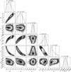 |
Fig. A.1 For DoAr 44, the joint posterior and marginalised probability distributions for the homogeneous ellipse model, based on VLTI/GRAVITY measurements, are presented. These parameters are α and β, describing the ellipse’s semi-major and semi-minor axes in milliarcseconds, ω describing the position angle of the ellipse, and fs, fc, fh giving the fractional contributions of the star, circumstellar matter and a diffuse, always resolved halo. Although some parameters exhibit strong correlations, this does not affect the usefulness of the calculations. The size of the ellipse (at 146 pc) is 0.2 × 0.24 au, and the contribution of the always-resolved halo is approximately 7%. The parameter uncertainties appear underestimated, likely due to the simplicity of the model. |
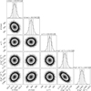 |
Fig. A.2 For DoAr 44, the joint posterior and marginalised probability distributions for the parameters of the δ-ring model describing the ALMA Band 7 data are presented. These parameters are α and β, describing the dimensions of the ellipse in milliarcseconds, ω, giving the position angle in degrees, and A and B, representing the fractional contribution of the unresolved and always-resolved emission, respectively. |
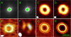 |
Fig. A.3 Comparison of available spatially resolved observations of DoAr 44. A: VLT/SPHERE/IRDIS Channel 1 (Avenhaus et al. 2018). B: VLT/SPHERE/IRDIS Channel 2 (Avenhaus et al. 2018). C: ALMA Band 3. Angular resolution: 0.251”. Project code: 2019.1.01111.S. D: ALMA Band 7.0.168” (Arce-Tord et al. 2023). E: ALMA Band 8. 0.154” (Casassus et al. 2023). F: SMA at 346 GHz. 0.41” (van der Marel et al. 2016). G: ALMA Band 7. 0.023” (Arce-Tord et al. 2023). H: ALMA Band 6. 0.026” (Cieza et al. 2021). The SPHERE images are in the H band, and correspond to perpendicular linear polarisations. The green circle on the SPHERE images is the 0.1 “radial extent of the coronagraph. Contours are plotted over the low-resolution interferometric images. The synthesised beam, corresponding to the angular resolution, is shown as a white ellipse (very small for plots G and H). The scale is consistent on all plots. These ALMA observations were also used to constrain the model of the SED. |
References
- Andrews, S. M., Wilner, D., Hughes, A., Qi, C., & Dullemond, C., 2009, ApJ, 700, 1502 [CrossRef] [Google Scholar]
- Andrews, S. M., Wilner, D. J., Hughes, A. M., Qi, C., & Dullemond, C. P., 2010, ApJ, 723, 1241 [Google Scholar]
- Andrews, S. M., Wilner, D. J., Espaillat, C., et al. 2011, ApJ, 732, 42 [Google Scholar]
- Andrews, S. M., Huang, J., Pérez, L. M., et al. 2018, ApJ, 869, L41 [NASA ADS] [CrossRef] [Google Scholar]
- Arce-Tord, C., Casassus, S., Dent, W. R., et al. 2023, MNRAS, 526, 2077 [NASA ADS] [CrossRef] [Google Scholar]
- Asplund, M., Grevesse, N., & Jacques Sauval, A., 2006, Nucl. Phys. A, 777, 1 [CrossRef] [Google Scholar]
- Avenhaus, H., Quanz, S. P., Garufi, A., et al. 2018, ApJ, 863, 44 [NASA ADS] [CrossRef] [Google Scholar]
- Bessell, M., Bloxham, G., Schmidt, B., et al. 2011, PASP, 123, 789 [Google Scholar]
- Benisty, M., Bae, J., Facchini, S., et al. 2021, ApJ, 916, L2 [NASA ADS] [CrossRef] [Google Scholar]
- Bessolaz, N., Zanni, C., Ferreira, J., Keppens, R., & Bouvier, J., 2008, A&A, 478, 155 [NASA ADS] [CrossRef] [EDP Sciences] [Google Scholar]
- Billot, N., Agnèse, P., Auguères, J.-L., et al. 2006, in Space Telescopes and Instrumentation I: Optical, Infrared, and Millimeter, 6265, SPIE, 81 [Google Scholar]
- Bohn, A., Benisty, M., Perraut, K., et al. 2022, A&A, 658, A183 [NASA ADS] [CrossRef] [EDP Sciences] [Google Scholar]
- Bouvier, J., Alecian, E., Alencar, S. H. P., et al. 2020a, A&A, 643, A99 [EDP Sciences] [Google Scholar]
- Bouvier, J., Perraut, K., Le Bouquin, J.-B., et al. 2020b, A&A, 636, A108 [NASA ADS] [CrossRef] [EDP Sciences] [Google Scholar]
- Brož, M., Chrenko, O., Nesvorný, D., & Dauphas, N., 2021, Nat. Astron., 5, 898 [CrossRef] [Google Scholar]
- Brož, M., Mourard, D., Budaj, J., et al. 2021, A&A, 645, A51 [EDP Sciences] [Google Scholar]
- Budaj, J., & Richards, M. T., 2004, Contrib. Astron. Observ. Skalnate Pleso, 34, 167 [Google Scholar]
- Casassus, S., Avenhaus, H., Pérez, S., et al. 2018, MNRAS, 477, 5104 [NASA ADS] [CrossRef] [Google Scholar]
- Casassus, S., Pérez, S., Osses, A., & Marino, S., 2019, MNRAS, 486, L58 [NASA ADS] [CrossRef] [Google Scholar]
- Casassus, S., Cieza, L., Cárcamo, M., et al. 2023, MNRAS, 526, 1545 [NASA ADS] [CrossRef] [Google Scholar]
- Cieza, L. A., González-Ruilova, C., Hales, A. S., et al. 2021, MNRAS, 501, 2934 [Google Scholar]
- Cook, A., Whittet, D., Shenoy, S., et al. 2011, ApJ, 730, 124 [Google Scholar]
- Dodson-Robinson, S. E., & Salyk, C., 2011, ApJ, 738, 131 [CrossRef] [Google Scholar]
- Doğan, S., Nixon, C., King, A., & Price, D. J., 2015, MNRAS, 449, 1251 [CrossRef] [Google Scholar]
- Espaillat, C., Calvet, N., D’Alessio, P., et al. 2007, ApJ, 670, L135 [Google Scholar]
- Espaillat, C., D’Alessio, P., Hernández, J., et al. 2010, ApJ, 717, 441 [Google Scholar]
- Fazio, G., Hora, J., Allen, L., et al. 2004, ApJSS, 154, 10 [NASA ADS] [CrossRef] [Google Scholar]
- Foreman-Mackey, D., Hogg, D. W., Lang, D., & Goodman, J., 2013, PASP, 125, 306 [Google Scholar]
- Freudling, W., Romaniello, M., Bramich, D., et al. 2013, A&A, 559, A96 [NASA ADS] [CrossRef] [EDP Sciences] [Google Scholar]
- Gaia Collaboration. 2018, VizieR Online Data Catalog, I/345 [Google Scholar]
- Gaia Collaboration. 2020, VizieR Online Data Catalog, I/350 [Google Scholar]
- Greenberg, J. M., 1998, A&A, 330, 375 [NASA ADS] [Google Scholar]
- Griffin, M. J., Abergel, A., Abreu, A., et al. 2010, A&A, 518, L3 [EDP Sciences] [Google Scholar]
- Hayashi, C., 1981, Progr. Theor. Phys. Suppl., 70, 35 [Google Scholar]
- Henden, A. A., Templeton, M., Terrell, D., et al. 2016, VizieR Online Data Catalog: II/336 [Google Scholar]
- Husser, T.-O., Wende-von Berg, S., Dreizler, S., et al. 2013, A&A, 553, A6 [NASA ADS] [CrossRef] [EDP Sciences] [Google Scholar]
- Jayasinghe, T., Kochanek, C., Stanek, K., et al. 2018, MNRAS, 477, 3145 [Google Scholar]
- Kaiser, N., Aussel, H., Burke, B. E., et al. 2002, in Survey and Other Telescope Technologies and Discoveries, 4836, SPIE, 154 [NASA ADS] [Google Scholar]
- Keppler, M., Benisty, M., Müller, A., et al. 2018, A&A, 617, A44 [NASA ADS] [CrossRef] [EDP Sciences] [Google Scholar]
- Köhler, M., Ysard, N., & Jones, A. P., 2015, A&A, 579, A15 [NASA ADS] [CrossRef] [EDP Sciences] [Google Scholar]
- Krijt, S., Ciesla, F. J., & Bergin, E. A., 2016, ApJ, 833, 285 [Google Scholar]
- Kuffmeier, M., Dullemond, C. P., Reissl, S., & Goicovic, F. G., 2021, A&A, 656, A161 [NASA ADS] [CrossRef] [EDP Sciences] [Google Scholar]
- Kurosawa, R., Romanova, M. M., & Harries, T. J., 2011, MNRAS, 416, 2623 [NASA ADS] [CrossRef] [Google Scholar]
- Lazareff, B., Berger, J. P., Kluska, J., et al. 2017, A&A, 599, A85 [NASA ADS] [CrossRef] [EDP Sciences] [Google Scholar]
- Leiendecker, H., Jang-Condell, H., Turner, N. J., & Myers, A. D., 2022, ApJ, 941, 172 [NASA ADS] [CrossRef] [Google Scholar]
- Li, M., & Xiao, L., 2016, ApJ, 820, 36 [NASA ADS] [CrossRef] [Google Scholar]
- Lynden-Bell, D., & Pringle, J. E., 1974, MNRAS, 168, 603 [Google Scholar]
- Martín-Doménech, R., Caro, G. M., Bueno, J., & Goesmann, F., 2014, A&A, 564, A8 [NASA ADS] [CrossRef] [EDP Sciences] [Google Scholar]
- Mohanty, S., Greaves, J., Mortlock, D., et al. 2013, ApJ, 773, 168 [NASA ADS] [CrossRef] [Google Scholar]
- Montmerle, T., Koch-Miramond, L., Falgarone, E., & Grindlay, J. E., 1983, ApJ, 269, 182 [Google Scholar]
- Mourard, D., Brož, M., Nemravová, J. A., et al. 2018, A&A, 618, A112 [NASA ADS] [CrossRef] [EDP Sciences] [Google Scholar]
- Mumma, M. J., & Charnley, S. B., 2011, Annu. Rev. Astron. Astrophys., 49, 471 [Google Scholar]
- Nealon, R., Cuello, N., & Alexander, R., 2019, MNRAS, 491, 4108 [Google Scholar]
- Nemravová, J., Harmanec, P., Brož, M., et al. 2016, A&A, 594, A55 [NASA ADS] [CrossRef] [EDP Sciences] [Google Scholar]
- Nesvorný, D., 2018, ARA&A, 56, 137 [CrossRef] [Google Scholar]
- Neugebauer, G., Habing, H., Van Duinen, R., et al. 1984, ApJ, 278, L1 [NASA ADS] [CrossRef] [Google Scholar]
- Nixon, C., King, A., & Price, D., 2013, MNRAS, 434, 1946 [NASA ADS] [CrossRef] [Google Scholar]
- Ochsenbein, F., Bauer, P., & Marcout, J., 2000, A&A Suppl. Ser., 143, 23 [Google Scholar]
- Page, M., Brindle, C., Talavera, A., et al. 2012, MNRAS, 426, 903 [NASA ADS] [CrossRef] [Google Scholar]
- Perotti, G., Christiaens, V., Henning, T., et al. 2023, Nature, 620, 516 [NASA ADS] [CrossRef] [Google Scholar]
- Pontoppidan, K. M., Salyk, C., Bergin, E. A., et al. 2014, Protostars and Planets VI, 363 [Google Scholar]
- Ricci, L., Testi, L., Natta, A., & Brooks, K. 2010a, A&A, 521, A66 [NASA ADS] [CrossRef] [EDP Sciences] [Google Scholar]
- Ricci, L., Testi, L., Natta, A., et al. 2010b, A&A, 512, A15 [CrossRef] [EDP Sciences] [Google Scholar]
- Rieke, G., Young, E., Engelbracht, C., et al. 2004, ApJ Suppl. Ser., 154, 25 [Google Scholar]
- Rubin, M., Altwegg, K., Berthelier, J.-J., et al. 2023, MNRAS, 526, 4209 [NASA ADS] [CrossRef] [Google Scholar]
- Salyk, C., Lacy, J. H., Richter, M. J., et al. 2015, ApJ, 810, L24 [NASA ADS] [CrossRef] [Google Scholar]
- Skrutskie, M., Cutri, R., Stiening, R., et al. 2006, AJ, 131, 1163 [Google Scholar]
- Takasao, S., Tomida, K., Iwasaki, K., & Suzuki, T. K., 2018, ApJ, 857, 4 [NASA ADS] [CrossRef] [Google Scholar]
- Takita, S., Kataza, H., Kitamura, Y., et al. 2010, A&A, 519, A83 [NASA ADS] [CrossRef] [EDP Sciences] [Google Scholar]
- van der Marel, N., 2023, Eur. Phys. J. Plus, 138, 225 [NASA ADS] [CrossRef] [Google Scholar]
- van der Marel, N., van Dishoeck, E. F., Bruderer, S., et al. 2016, A&A, 585, A58 [NASA ADS] [CrossRef] [EDP Sciences] [Google Scholar]
- Wright, E. L., Eisenhardt, P. R., Mainzer, A. K., et al. 2010, AJ, 140, 1868 [Google Scholar]
- York, D. G., Adelman, J., AndersonJr, J. E., et al. 2000, AJ, 120, 1579 [NASA ADS] [CrossRef] [Google Scholar]
- Ysard, N., Jones, A., Demyk, K., Boutéraon, T., & Koehler, M., 2018, A&A, 617, A124 [NASA ADS] [CrossRef] [EDP Sciences] [Google Scholar]
- Zak, J., Bocchieri, A., Sedaghati, E., et al. 2024, A&A, 686, A147 [NASA ADS] [CrossRef] [EDP Sciences] [Google Scholar]
- Zhang, K., Pontoppidan, K. M., Salyk, C., & Blake, G. A., 2013, ApJ, 766, 82 [NASA ADS] [CrossRef] [Google Scholar]
- Zhou, Y., Bowler, B. P., Wagner, K. R., et al. 2021, AJ, 161, 244 [NASA ADS] [CrossRef] [Google Scholar]
All Tables
Best-fit parameters of the homogeneous ellipse model suitable for the VLTI measurements of the accretion region.
Best-fit parameters of the elliptical δ-ring model, suitable for the ALMA visibilities.
All Figures
|
Fig. 1 Individual VLT Hα spectra of DoAr 44 and a mean spectrum. The spectrum is temporally variable, so a mean spectrum is used to constrain the mean state of the system. |
| In the text | |
|
Fig. 2 VLTI/GRAVITY K-band interferometric visibilities of DoAr 44. Left: UV coverage of the observations in M λ. Right: squared visibility as a function of UV distance ( |
| In the text | |
|
Fig. 3 ALMA Band 7 Squared visibilites of DoAr 44 for both polarisations (XX, YY) plotted separately as a function of uv-distance in Mλ. |
| In the text | |
|
Fig. 4 Left: Synthetic image of the accretion region, in the 2 μm continuum. Centre: fit of VLTI/GRAVITY squared visibilities. Right: fit of the averaged Hα profile. The blue region is the standard deviation of the VLT spectra, representing the temporal variability. |
| In the text | |
|
Fig. 5 Left: synthetic image in the 870 μm continuum of the best-fit model of the outer disc of DoAr44. Right: fit of the ALMA Band 7 squared visibilities. |
| In the text | |
|
Fig. 6
|
| In the text | |
|
Fig. 7 SED measurements of DoAr 44 and a synthetic SED, made up of several components. The central star and accretion region dominate in the ultraviolet and visible range, and the outer disc is dominant in the sub-millimetre and millimetre wavelengths. These two contributions are well constrained from VLTI and ALMA interferometry. However, if only these two components are considered, a large deficit is present in the mid-infrared range. Therefore, an intermediate region must be present. The error bars are not visible, as the vertical axis spans ten magnitudes. |
| In the text | |
|
Fig. 8 Total (gas + dust) density and temperature profiles of DoAr44, with the assumed metallicity of Z=0.0122. The model is composed of four segments (from left to right): 1. A hot optically thin shell where Hα emission originates; 2. An innermost disc, which presumably feeds the accretion shell; 3. An intermediate disc, necessary to explain the SED in the mid-IR region; 4. A cold outer disc, visible with the ALMA. Between the intermediate and the outer disc, a large ≈ 30 au cavity is present. |
| In the text | |
|
Fig. A.1 For DoAr 44, the joint posterior and marginalised probability distributions for the homogeneous ellipse model, based on VLTI/GRAVITY measurements, are presented. These parameters are α and β, describing the ellipse’s semi-major and semi-minor axes in milliarcseconds, ω describing the position angle of the ellipse, and fs, fc, fh giving the fractional contributions of the star, circumstellar matter and a diffuse, always resolved halo. Although some parameters exhibit strong correlations, this does not affect the usefulness of the calculations. The size of the ellipse (at 146 pc) is 0.2 × 0.24 au, and the contribution of the always-resolved halo is approximately 7%. The parameter uncertainties appear underestimated, likely due to the simplicity of the model. |
| In the text | |
|
Fig. A.2 For DoAr 44, the joint posterior and marginalised probability distributions for the parameters of the δ-ring model describing the ALMA Band 7 data are presented. These parameters are α and β, describing the dimensions of the ellipse in milliarcseconds, ω, giving the position angle in degrees, and A and B, representing the fractional contribution of the unresolved and always-resolved emission, respectively. |
| In the text | |
|
Fig. A.3 Comparison of available spatially resolved observations of DoAr 44. A: VLT/SPHERE/IRDIS Channel 1 (Avenhaus et al. 2018). B: VLT/SPHERE/IRDIS Channel 2 (Avenhaus et al. 2018). C: ALMA Band 3. Angular resolution: 0.251”. Project code: 2019.1.01111.S. D: ALMA Band 7.0.168” (Arce-Tord et al. 2023). E: ALMA Band 8. 0.154” (Casassus et al. 2023). F: SMA at 346 GHz. 0.41” (van der Marel et al. 2016). G: ALMA Band 7. 0.023” (Arce-Tord et al. 2023). H: ALMA Band 6. 0.026” (Cieza et al. 2021). The SPHERE images are in the H band, and correspond to perpendicular linear polarisations. The green circle on the SPHERE images is the 0.1 “radial extent of the coronagraph. Contours are plotted over the low-resolution interferometric images. The synthesised beam, corresponding to the angular resolution, is shown as a white ellipse (very small for plots G and H). The scale is consistent on all plots. These ALMA observations were also used to constrain the model of the SED. |
| In the text | |
Current usage metrics show cumulative count of Article Views (full-text article views including HTML views, PDF and ePub downloads, according to the available data) and Abstracts Views on Vision4Press platform.
Data correspond to usage on the plateform after 2015. The current usage metrics is available 48-96 hours after online publication and is updated daily on week days.
Initial download of the metrics may take a while.