| Issue |
A&A
Volume 701, September 2025
|
|
|---|---|---|
| Article Number | A181 | |
| Number of page(s) | 14 | |
| Section | Extragalactic astronomy | |
| DOI | https://doi.org/10.1051/0004-6361/202553788 | |
| Published online | 12 September 2025 | |
The 10 kpc collar of early-type galaxies: Probing evolution by focusing on the inner stellar density profile
1
Department of Astronomy, School of Physics and Astronomy, Shanghai Jiao Tong University, Shanghai 200240, China
2
Shanghai Key Laboratory for Particle Physics and Cosmology, Shanghai Jiao Tong University, Shanghai 200240, China
3
Key Laboratory for Particle Physics, Astrophysics and Cosmology, Ministry of Education, Shanghai Jiao Tong University, Shanghai 200240, China
4
Dipartimento di Fisica e Astronomia “Augusto Righi”, Alma Mater Studiorum – Universitá di Bologna, Via Gobetti 93/2, 40129 Bologna, Italy
5
Institute for Astrophysics, School of Physics, Zhengzhou University, Zhengzhou 450001, China
⋆ Corresponding authors: This email address is being protected from spambots. You need JavaScript enabled to view it.
, This email address is being protected from spambots. You need JavaScript enabled to view it.
Received:
17
January
2025
Accepted:
17
July
2025
Abstract
Context. The post-quenching evolution process of early-type galaxies (ETGs), which is typically driven by mergers, is still not fully understood. The amount of growth in stellar mass and size incurred after quenching is still under debate.
Aims. In this work, we investigated the late evolution of ETGs, both observationally and theoretically, by focusing on the stellar mass density profile inside a fixed aperture, within 10 kpc from the galaxy center.
Methods. We first studied the stellar mass and the mass-weighted density slope within 10 kpc, respectively M*, 10 and Γ*, 10, of a sample of ETGs from the GAMA survey. We measured the Γ*, 10 − M*, 10 relation and its evolution over the redshift range 0.17 ≤ z ≤ 0.37. We then built a toy model for the merger evolution of galaxies, based on N-body simulations, to explore to what extent the observed growth in Γ*, 10 − M*, 10 relation is consistent with a dry-merger evolution scenario.
Results. From the observations, we do not detect evidence for an evolution of the Γ*, 10 − M*, 10 relation relation. We put an upper limit on the redshift derivative of the normalization (μ) and slope (β) of the Γ*, 10 − M*, 10 relation: |∂μ/∂log(1 + z)| ≤ 0.13 and |∂β/∂log(1+z)| ≤ 1.10, respectively. Simulations show that most mergers induce a decrease in Γ*, 10 and an increase in M*.10, although some show a decrease in M*, 10, particularly for the most extended galaxies and smaller merger mass ratios. By combining the observations with our merger toy model, we place an upper limit on the fractional stellar mass growth of fM = 11.2% in the redshift range 0.17 ≤ z ≤ 0.37.
Conclusions. While our measurement is limited by systematics, the application of our approach to samples with a larger redshift baseline, particularly with a time interval Δt ≥ 3.2 Gyr, should enable detection of a signal and improves our understanding of the late growth of ETGs.
Key words: galaxies: elliptical and lenticular / cD / galaxies: evolution / galaxies: fundamental parameters / galaxies: structure
© The Authors 2025
 Open Access article, published by EDP Sciences, under the terms of the Creative Commons Attribution License (https://creativecommons.org/licenses/by/4.0), which permits unrestricted use, distribution, and reproduction in any medium, provided the original work is properly cited.
This article is published in open access under the Subscribe to Open model. This email address is being protected from spambots. You need JavaScript enabled to view it. to support open access publication.
1. Introduction
Early-type galaxies (ETGs), which are typically elliptical in shape and evolve passively, are believed to represent the final stage of galaxy evolution. By the time they are observed, these galaxies have likely completed most of their star formation activity. However, they may still undergo further evolution via mergers and accretion. Understanding the post-quenching evolution process that ETGs undergo can provide insight into the hierarchical structure formation theory, which is fundamental in the context of the lambda cold dark matter (ΛCDM) cosmology.
Observations suggest that ETGs at higher redshift (i.e. z ≈ 2) have significant differences from their z ≈ 0 counterparts in several aspects. For instance, ETGs at z ≈ 2 are more compact in size (e.g. Daddi et al. 2005; Toft et al. 2007; Trujillo et al. 2006, 2007; van Dokkum et al. 2008) and have smaller color gradients, i.e., the contrast in color between the outskirt and the center is less significant than that of their low-redshift counterparts (e.g. Suess et al. 2019a,b, 2020). Specifically, the apparent size growth at fixed mass of such quiescent, compact objects is believed to be a factor of approximately three between z = 2 and z = 0 (e.g. Fan et al. 2008; van Dokkum et al. 2010; van der Wel et al. 2014; Damjanov et al. 2019; Hamadouche et al. 2022). Combined with the relatively low star-formation rate of ETGs, this suggests that these galaxies have been building up their outer envelopes since z ≈ 1.5 via some form of merging and accretion (e.g. Hopkins et al. 2009, 2010; van Dokkum et al. 2010). Numerous studies based on both observations and hydrodynamical simulations suggest that, among various possible mechanisms, the dominant one is dissipationless (dry) mergers, especially those with a relatively small mass ratio between the accreted galaxy and the progenitor galaxy (hereafter minor mergers). The rationale is that minor mergers can produce the largest growth in size for the same accreted mass and qualitatively reproduce the evolutionary trend in central densities and orbital structures of these quiescent galaxies (e.g. Naab et al. 2009; van Dokkum & Brammer 2010; Oser et al. 2011; Newman et al. 2012; Hilz et al. 2013; Dekel & Burkert 2014; D’Eugenio et al. 2023). Recently, taking advantage of the depth and resolution of the James Webb Space Telescope Advanced Deep Extragalactic Survey (Gardner et al. 2023; Eisenstein et al. 2023), Suess et al. (2023) suggested that minor mergers also have the potential to contribute to the color gradient evolution of ETGs.
Nevertheless, a quantitative investigation of the evolutionary process reveals that the minor merger scenario is insufficient to explain the full growth of ETGs at redshift z > 1. Studies based on HST images (e.g. Newman et al. 2012; Belli et al. 2015) identify satellite galaxies around massive ETGs and find that the merging event of ETGs with their surrounding satellites can account for at most half of the entire size growth. Moreover, studies based on theoretical models (e.g. Nipoti et al. 2009a,b, 2012) also imply that it is difficult to reproduce the evolution of the Re − M* relation, i.e., the relation between the half-light radius, Re, and the total stellar mass, M*, by solely invoking dry mergers. Some possible solutions to this problem have already been proposed. Given that the observed size of star-forming galaxies is on average larger than that of quiescent ones (e.g. Newman et al. 2012; van der Wel et al. 2014; Belli et al. 2015; Roy et al. 2018), the addition of newly quenched ex-star-forming galaxies to the population of ETGs could supplement the size growth of ETGs (e.g. Dokkum & Franx 1996; van Dokkum & Franx 2001; Carollo et al. 2013; Fagioli et al. 2016). The existence of color gradients could also mimic the observed size growth of ETGs, thus misleading to a conclusion that the minor merger scenario is insufficient (Suess et al. 2019a,b). Detailed theoretical models that incorporate various possible scenarios and explain the entire growth of ETGs are still lacking. It must also be noted that the evolution of other scaling relations (such as those involving the central stellar velocity dispersion) provides additional and complementary constraints on such models (Cannarozzo et al. 2020; Nipoti 2025).
Another problem arises at lower redshift, z ≤ 1, where there is not yet a consensus on the observed evolution of ETGs. The growth rate of ETGs at that time appears to be mass-dependent. van der Wel et al. (2014), Roy et al. (2018) suggested a more rapid size growth rate for more massive ETGs (M* ≥ 1011 M⊙), but Damjanov et al. (2019) find that less massive ETGs tend to grow faster. Moreover, studies exploring the number density growth of ETGs (e.g. Bundy et al. 2017; Kawinwanichakij et al. 2020) imply a lack of growth in the stellar mass function in the same redshift interval, which is generally in agreement with Damjanov et al. (2019) as both imply that massive ETGs do not grow significantly, and thus contrast with van der Wel et al. (2014) and Roy et al. (2018). Such complexity limits our ability to draw precise conclusions about the evolution of ETGs in this redshift range. Whether ETGs grow in this redshift range is still not determined, let alone the detailed growth mechanism.
So far, ETG evolution has mainly been studied by means of the total stellar mass, M*, and the half-light radius, Re. However, the full light (stellar) profile contains more information than can be compressed into these two quantities. Indeed, efforts have been made to extract the light profile to the faint outer region and study the evolution of the stellar halo (e.g. Tal & van Dokkum 2011; D’Souza et al. 2014; Huang et al. 2018, 2020; Spavone et al. 2021; Chen et al. 2022; Williams et al. 2025). The outer stellar distribution is believed to preserve information about the accretion history of galaxies, with flatter light profiles indicating a larger fraction of accreted stellar mass. In this work, we chose a complementary approach, by focusing on the inner region of ETGs and their evolution.
Following Sonnenfeld (2020), we defined the inner region as the region inside a circularized radius, 10 kpc, and described the stellar density profile using the mass (M*, 10) and mass-weighted density slope (Γ*, 10) enclosed within that aperture. The mass-weighted density slope is defined as
 (1)
(1)
where radii are expressed in kiloparsecs. These two parameters provide a good summary of the inner stellar distribution of ETGs, in the sense that by specifying their values, we can predict the stellar profile inside 10 kpc to better than 20% (see Fig. 8 in Sonnenfeld 2020). Therefore, we refer to these two parameters as the 10 kpc collar. The choice of 10 kpc is arbitrary, but it represents a compromise between a scale that is sufficiently large enough to enclose a substantial fraction of the mass of a massive ETG, but not so large that this fraction becomes one. A benefit of using this parametrization is that it does not suffer from extrapolation problems: at the redshifts and depths covered by our study, the surface brightness of ETGs is detected out to 10 kpc, and therefore M*, 10 and Γ*, 10 can be measured directly from the data. In contrast, obtaining M* and Re requires extrapolating the surface brightness model distribution to regions below the sky background level. As shown by Sonnenfeld (2020), this extrapolation can be significant even at relatively low redshifts, z ∼ 0.2.
Using our new robust parametrization, we measured the evolution of the inner stellar density profile of ETGs in the redshift range 0.15 ≤ z ≤ 0.40. We first collected a sample of quiescent galaxies, measured their M*, 10 and Γ*, 10, and then analyzed the evolution of the Γ*, 10 − M*, 10 relation. Furthermore, to explore the extent to which the evolution of this Γ*, 10 − M*, 10 relation can be explained by dry mergers, we utilized the set of simulations used in Sonnenfeld et al. (2014) and originally presented in Nipoti et al. (2009b, 2012), which contains a number of binary merger simulations with different merger mass ratios. We used fM, the fractional stellar mass growth of galaxies, to represent the growth of ETGs driven by dry mergers, and built a toy model to estimate the maximum fM allowed by the observed evolution in the Γ*, 10 − M*, 10 relation in the redshift range 0.15 ≤ z ≤ 0.40.
The structure of this paper is as follows. We describe the observation sample together with the measurement of M*, 10 and Γ*, 10 in Sect. 2. In Sect.3, we present the measurement of the Γ*, 10 − M*, 10 relation using a Bayesian hierarchical method and in Sect. 4, we describe how we establish a toy model based on simulations to find a maximum fractional mass growth fM that is allowed by the observed evolution of the Γ*, 10 − M*, 10 relation, in the context of dry mergers. We discuss the results in Sect. 5 and provide a brief conclusion in Sect. 6.
We assume a flat ΛCDM cosmology with ΩM = 0.3 and H0 = 70 km s−1 Mpc−1. Magnitudes are in AB units and stellar masses are in solar units.
2. Observations
2.1. Sample selection
The goal of this work was to investigate the evolution of quiescent galaxies at low redshift and to attempt to eliminate possible systematic effects from the extrapolation problem by focusing on a fixed aperture size of 10 kpc. We selected a sample consisting of quiescent galaxies with spectroscopic data, thereby obtaining reliable measurements of redshift, stellar mass, and aperture size and distinguishing them from star-forming galaxies. In particular, we required the method for stellar mass measurement to be homogeneous throughout the whole sample. In addition, we needed to obtain the structural parameters of galaxies to calculate M*, 10 and Γ*, 10.
Therefore, we selected galaxies based on the Galaxy And Mass Assembly Data Release 4 (GAMA DR4, Baldry et al. 2010; Hopkins et al. 2013; Bellstedt et al. 2020; Driver et al. 2022). Specifically, we used the data management unit (DMU) gkvScienceCatv02 (Bellstedt et al. 2020) to select galaxies brighter than an r-band ProFound magnitude of 19.65 from the GAMA DR4 Main Survey sample, which has a 95% spectroscopic completeness. We conservatively included only galaxies in the G09, G12, and G15 fields, due to the shallower r-band magnitude limit in the G23 field. We obtained stellar mass measurements from the DMU StellarMassesGKVv24 (see Driver et al. 2022). Stellar masses were estimated using stellar population synthesis (SPS) modeling to the observed spectral energy distribution (SED) data. The fitting code was first described in Taylor et al. (2011), and later modified to operate within a fixed wavelength range of 3000–11 000 Å. The fitting used the stellar evolution models of Bruzual & Charlot (2003), assuming a Chabrier (2003) stellar initial mass function (IMF), uniform metallicity, exponentially declining star formation histories, and the dust curve of Calzetti et al. (2000). The main reference for the measurement is Taylor et al. (2011), while the photometric data used in this stellar mass estimation procedure are from Bellstedt et al. (2020).
To select ETGs, we used the spectroscopic index Dn4000 to distinguish the quiescent galaxies. In GAMA, this index follows the narrow-band definition of Balogh et al. (1999), which is defined as the ratio between the flux per unit frequency in 4000 − 4100 Å and 3850 − 3950 Å. This index is commonly used as an indicator of the age of the stellar population. According to Kauffmann et al. (2003), the distribution of Dn4000 exhibits strong bimodality with a clear division between star-forming and quiescent galaxies at Dn4000 = 1.5. Therefore, we applied a selection criterion of Dn4000 > 1.5 to select quiescent galaxies. We also removed galaxies with normalized redshift quality nQ ≤ 2, following the suggestion of the GAMA Collaboration (Driver et al. 2022).
In addition, we included only galaxies that overlap with the Kilo-Degree Survey (KiDS, de Jong et al. 2013; Kuijken et al. 2019), in order to obtain surface brightness profiles of our galaxies. Galaxy structural parameters were measured using GalNet (Li et al. 2022), which fits single Sérsic models to the surface brightness of KiDS DR5 galaxies using its r-bandphotometry. After excluding galaxies with catastrophic measurements, the final sample comprised 66 145 ETGs with measurement of spectroscopic redshift, stellar mass, and structural parameters.
2.2. Measurement of M*, 10 and Γ*, 10
To obtain M*, 10 and Γ*, 10 for the galaxies in our sample, we fit the image of galaxies with a point spread function (PSF)-convolved Sérsic model, then derived the M*, 10 and Γ*, 10 based on the best-fitting model. While the total mass, M*, and half-light radius, Re, derived by fitting a Sérsic model suffer from the extrapolation problem discussed in Sect. 1, the quantities M*, 10 and Γ*, 10 do not. This is because, as we show below, the surface brightness profile in the inner 10 kpc is well constrained by our data and is well described by our best-fitting Sérsic model. Although, in principle, M*, 10 and Γ*, 10 could be determined in a nonparametric way by directly measuring the surface brightness profile, our model-based approach allowed us to more conveniently deblend the galaxies of interest from contaminants and to deconvolve the surface brightness profile by the PSF (see Li et al. 2022, for details).
The Sérsic profile (Sersic 1968) can be written as
 (2)
(2)
with
 (3)
(3)
Here, q is the axis ratio, n is the Sérsic index, and R is the circularized radius where x and y are Cartesian coordinates with origin at the center of galaxies. We use the symbol x to denote the axis aligned with the semi-major axis of the ellipse, while using y to denote the axis aligned with the semi-minor axis. The effective radius, Re, is also circularized. The light enclosed within a circularized aperture of radius R is given by
![Mathematical equation: $$ \begin{aligned} L( < R) = 2\pi n\cdot I_0R_{\rm e}^2 \cdot \frac{1}{\left(b_n\right)^{2n}}\cdot \gamma \left[2n,b_n \left(\frac{R}{R_{\rm e}}\right)^{\frac{1}{n}}\right]. \end{aligned} $$](/articles/aa/full_html/2025/09/aa53788-25/aa53788-25-eq4.gif) (4)
(4)
The total light can be obtained by letting R → +∞,
 (5)
(5)
Here Γ is the gamma function, γ is the lower incomplete gamma function, and bn is a constant that ensures the light enclosed within the effective radius, Re, is half of the total light:
 (6)
(6)
Therefore, bn can be calculated by solving
 (7)
(7)
To demonstrate the accuracy of our Sérsic fits in the inner 10 kpc region, we show in Fig. 1 a comparison between the PSF-convolved best-fitting model surface brightness profiles and the circularized surface brightness profiles measured in radial bins directly from the data, for 25 galaxies. We selected these galaxies randomly, while discarding objects with bright companions. We applied this additional isolation cut only to illustrate Fig. 1. As shown by Li et al. (2022), our fitting method can handle objects with overlapping surface brightness distributions, and such objects are included in our analysis. However, the presence of neighbors complicates the procedure of measuring the surface brightness profile directly from the data, and thus complicates our comparison. The observed light profile can be reproduced by the best-fitting Sérsic model inside 10 kpc (denoted by the vertical dashed pink line) with a typical accuracy of 10%. Residuals are thus much smaller than the uncertainties on the stellar mass-to-light ratio, which are on the order of 30%. Therefore, our measurements of M*, 10 and Γ*, 10 are largely immune to the impact of systematics related to the determination of galaxy structural parameters. Additionally, we measured the median fractional error across the 25 galaxies, finding values of 1.2% for the surface brightness at 10 kpc and 1.5% for the enclosed light within the same radius. These results confirm that the best-fitting model provides an unbiased reconstruction of the surface brightness profile, thereby ensuring the reliability of the derived parameters M,10 and Γ,10. Figure 1 also shows that the radius at which the surface brightness of our galaxies falls below the sky background root mean square (rms) level (horizontal dashed line) is typically larger than 10 kpc. This means that M*, 10 and Γ*, 10 are indeed determined directly from the data and thus do not suffer from the extrapolation problem.
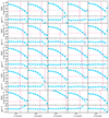 |
Fig. 1. Surface brightness profile of 25 galaxies. These galaxies were selected after visually inspecting 69 galaxies in one KiDS tile and randomly choosing 25 from the 62 without bright companions. The upper panel shows the surface brightness as a function of the circularized radius. The solid blue line shows the best-fitting Sérsic model convolved with PSF, calculated using GalNet structural parameters. The blue diamonds show measurements directly obtained from the KiDS r-band image. The lower panel shows the difference between the two measurements. The vertical dashed pink line indicates the angular size corresponding to 10 kpc for each galaxy. The horizontal line represents the noise level of the sky. |
In this work, we assume that there is no stellar mass-to-light ratio gradient within individual galaxies; hence, the stellar mass profile can be obtained directly from the light profile. We discuss the possible implications of this choice in Sect. 5.2. We obtained the stellar mass estimate for each galaxy from GAMA, along with the light used in the SPS model fitting process (Driver et al. 2022), which enabled us to calculate the mass-to-light ratio, Υ*. The mass profile can be easily obtained by multiplying Eqs. (2) and (4) by Υ*:
![Mathematical equation: $$ \begin{aligned} \Sigma _*(R) = \Upsilon _* I_0 \exp \left[-b_n\left(\frac{R}{R_{\rm e}}\right)^{1/n}\right], \end{aligned} $$](/articles/aa/full_html/2025/09/aa53788-25/aa53788-25-eq8.gif) (8)
(8)
![Mathematical equation: $$ \begin{aligned} M_*( < R) = \Upsilon _* 2\pi n\cdot I_0R_{\rm e}^2 \cdot \frac{1}{\left(b_n\right)^{2n}}\cdot \gamma \left[2n,b_n \left(\frac{R}{R_{\rm e}}\right)^{\frac{1}{n}}\right]. \end{aligned} $$](/articles/aa/full_html/2025/09/aa53788-25/aa53788-25-eq9.gif) (9)
(9)
By substituting R = 10 kpc into Eq. (9), we obtained M*, 10, while we obtained Γ*, 10 by combining Eq. (8) with Eq. (1).
The stellar mass-to-light ratio, Υ*, and the Sérsic structural parameters, Re and n, are measured by two different surveys: the Υ* ratio from GAMA, and Re and n from KiDS. Since the total flux of a galaxy used in KiDS Sérsic modeling may differ from that used in the GAMA stellar mass estimate, this discrepancy must be taken into account when deriving M*, 10 and Γ*, 10. However, because we assumed that there is no gradient in the stellar mass-to-light ratio, the measured value of Υ* does not depend on the modeling choice. Therefore, although Υ* can only be obtained from the GAMA survey, we believe that it is reasonable to use it to calculate M*, 10 and Γ*, 10 together with the structure parameter measured by KiDS.
2.3. Completeness
To minimize potential biases related to selection effects, we constructed a volume-limited sample in M*, 10. The GAMA DR4 Main Survey sample, from which the quiescent galaxies were selected, is flux-limited, with a 95% completeness limit down to an r-band ProFound magnitude of 19.65, which corresponds to a critical flux Fcrit ≈ 5.01 × 10⁻⁵ Jy. To obtain a complete M*, 10 sample, we needed to translate this flux-completeness limit into a limit in M*, 10.
We used the M*, 10-to-flux ratio to perform this translation. At a given redshift, the ratio between M*, 10 and the total flux, F, is not a fixed value, but rather is spread over a relatively wide range. We divided the sample into narrow redshift bins, measured the distribution of M*, 10/F in each bin, and found the critical value M*, 10/F|crit, where the cumulative probability reaches 95%. Multiplying M*, 10/F|crit by the critical flux Fcrit, we obtained the M*, 10 limit for that redshift bin. Here, we made an implicit assumption that the ratio M*, 10/F depends neither on M*, 10 nor on F.
Fig. 2 illustrates the procedure, which shows the distribution of M*, 10/F in three different redshift bins, with dashed lines indicating the 95th percentile of each bin, i.e., the critical M*, 10-to-flux ratio M*, 10/F|crit. The  in these three bins is calculated by
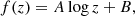
  , using the value of M*, 10/F|crit in each bin. Applying this procedure iteratively across all redshift bins results in the full 95% completeness limit in M*, 10 as a function of redshift z. We used a logarithmic formula to fit this limit as a function of redshift:
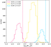 |
Fig. 2. Distribution of M*, 10/F in three narrow redshift bins. The vertical dashed line marks the 95th percentile of the distribution in each bin. By multiplying this ratio by the flux corresponding to the r-band magnitude limit, rcrit = 19.65, we obtain the M*, 10 limit for that redshift bin. |
 (10)
(10)
where the best-fitting parameters are A = 0.87 ± 0.0001 and B = 11.74 ± 0.0003.
The upper panel of Fig. 3 shows the distribution of our sample in M*, 10 − z space, with the solid pink line showing the 95% completeness limit. Galaxies with M*, 10 above this limit have a 95% probability of inclusion in our sample. Galaxies with M*, 10 below this limit were excluded and are shown as gray dots, while those included in the complete sample are shown as black dots. The lower panel shows the full sample in M* − z space with black dots.
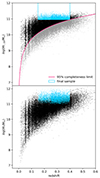 |
Fig. 3. Distribution of our galaxy sample in z − M*, 10 space (top) and z − M* space (bottom). The 95% completeness M*, 10 limit as a function of redshift of our ETG sample is shown by the solid pink line. Galaxies above this pink line, shown as black dots, are included in our complete sample; gray dots below the line are excluded. We further define lower and upper redshift limits of z ≥ 0.15 and z ≤ 0.40, respectively, to build the final sample shown as blue dots. |
We focused only on massive quiescent galaxies whose M*, 10 ≥ 1010.9 M⊙, and so imposed a corresponding upper redshift limit of z = 0.4. We further set a lower limit on the redshift range z ≥ 0.15, to increase the S/N with a reliably large sample size. The final sample used to investigate the evolution contained 5690 ETGs, shown as cyan dots in the upper panel of Fig. 3. The distribution of our final sample in the z − M* space is shown in the lower panel, with cyan dots representing the selected galaxies and black dots indicating the rest. The 5th percentile of the stellar mass distribution of our final sample is log M* = 11.1. The distribution of our sample in M*, 10, Γ*, 10, and z is shown in Fig. 4.
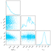 |
Fig. 4. Distribution of our 5690 ETGs in M*, 10, Γ*, 10, and redshift z. |
3. Γ*, 10 − M*, 10 relation
3.1. Model
Having obtained the measurements of M*, 10 and Γ*, 10, we proceeded to measure the Γ*, 10 − M*, 10 relation. We expected that this relation would provide valuable information on the growth of ETGs, complementary to the traditional Re − M* scaling relation. To infer the distribution of Γ*, 10 as a function of M*, 10, we fitted a model with a Bayesian hierarchical method. Each galaxy in our sample can be described by a set of quantities {log M*, 10, Γ*, 10, z}. The true values of these quantities, hereafter represented by Θ, are drawn from a probability distribution that correlates with the observed data  , which itself is described by a set of hyperparameters Φ. We wanted to obtain the posterior distribution of the hyperparameters Φ given the observed data d:
 (11)
(11)
and thus we marginalized every possible value of Θ in the likelihood term:
 (12)
(12)
The likelihood term on the right-hand side of Eq. (12) can be rewritten as
 (13)
(13)
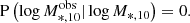
P(d|Θ) corresponds to the uncertainties of log M*, 10, Γ*, 10 and z. In this work, we only consider the uncertainty from the measurement of the stellar mass. Uncertainties from other sources are sufficiently small to be ignored. For example, P(zobs|z) is a negligible term as it is only affected by uncertainties on the spectroscopic redshift. The term  can also be ignored: Γ*, 10 does not depend on stellar mass, the measurement of the surface brightness profile is the only source of uncertainty, which is negligible as shown in Fig. 1. The remaining term of P(d|Θ) is
  , which we assumed to be a truncated Gaussian distribution, since we only selected galaxies whose
  . When
  , we have
![Mathematical equation: $$ \begin{aligned} \mathrm{P}\left(\log M_{*,10}^\mathrm{obs}|\log M_{*,10}\right)&= \frac{\mathcal{A} [\log M_{*,10}]}{\sqrt{2\pi \sigma ^2_{M_{*,10,obs}}}} \nonumber \\&\times \exp \left\{ -\frac{[\log M_{*,10} - \log M_{*,10}^\mathrm{obs}]^2}{2\sigma _{M_{*,10, obs}}^2}\right\} , \end{aligned} $$](/articles/aa/full_html/2025/09/aa53788-25/aa53788-25-eq21.gif) (14)
(14)
otherwise,
 (15)
(15)
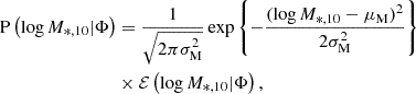
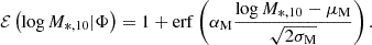
The factor 𝒜[log M*, 10] is a normalization constant that ensures that the probability of obtaining any log M*, 10 measurement larger than log M*, 10, min, given that a galaxy is part of our sample, is one. Therefore, the following equation for 𝒜 must be satisfied:
![Mathematical equation: $$ \begin{aligned} \int _{\log M_{*,10,\mathrm{min}}}^\infty \mathrm{d}\log M_{*,10}^\mathrm{obs}&\frac{\mathcal{A} [\log M_{*,10}]}{\sqrt{2\pi \sigma ^2_{M_{*,10,obs}}}} \nonumber \\&\times \exp \left\{ -\frac{[\log M_{*,10} - \log M_{*,10}^\mathrm{obs}]^2}{2\sigma _{M_{*,10, obs}}^2}\right\} = 1. \end{aligned} $$](/articles/aa/full_html/2025/09/aa53788-25/aa53788-25-eq23.gif) (16)
(16)
The second term on the right-hand side of Eq. (12) can be rewritten as
 (17)
(17)
This term formed the core of our model, as it contains both the distribution of log M*, 10 and also the relation between log M*, 10 and Γ*, 10. We wanted to fully capture both the average Γ*, 10 − M*, 10 relation and its redshift evolution. We chose a model-independent approach to describe the redshift evolution, aiming to avoid potential bias that might be introduced by an inadequate choice of functional form. We separated the sample into different redshift bins and, for each bin, fit the model while ignoring the redshift dependence of Γ*, 10.
The description of this model is as follows. Without the redshift dependence, Eq. (17) can be simplified to
 (18)
(18)
For the distribution of log M*, 10, we used a skewed normal distribution, inspired by the functional form used by Cannarozzo et al. (2020):
 (19)
(19)
where
 (20)
(20)
The function P(log M*, 10|Φ) serves as a prior on log M*, 10. Although a functional form of the skewed Gaussian distribution may not perfectly describe the log M*, 10 distribution, this issue does not significantly bias the posterior distribution. Adopting a Schechter function for the prior can only shift the mean and the standard deviation of the posterior distribution by no more than 0.01 dex and 1%, respectively. Since the uncertainty on log M*, 10 is smaller than the width of the log M*, 10 distribution, the posterior distribution is dominated by the second term, i.e., the likelihood part. The influence of the prior is therefore minimal. In addition, our model automatically corrected for the so-called Eddington bias.
For the distribution of Γ*, 10, we adopted a Gaussian model:
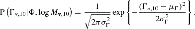 (21)
(21)
We modeled the relation between log M*, 10 and Γ*, 10 by a linear dependence of μΓ on log M*, 10:
 (22)
(22)
where the pivot value log M*, 10 = 11.04, which is the median value of M*, 10 of our sample.
Therefore, in this model, the full distribution of Θ given Φ is governed by the following set of hyperparameters:
 (23)
(23)
3.2. Fitting result
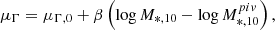
We binned our sample into four redshift bins of equal width and then sampled the posterior distribution of the hyperparameters in each bin. Table 1 shows the median value of the marginal posterior probability for each parameter. To illustrate the Γ*, 10 − M*, 10 relation, which is described by Eq. (22), we plot μΓ as a function of log M*, 10 in Fig. 5 as a dotted line, while the shaded region represents the 68% credible interval, according to the posterior probability. We also show the posterior distribution of these hyperparameters that govern the Γ*, 10 − M*, 10 relation in Fig. 6, with four different colors representing the four redshift bins.
Median values of the marginal posterior probability of the model parameters in each redshift bin.
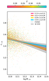 |
Fig. 5. The Γ*, 10 − M*, 10 relation of our observation sample fitted using a Bayesian hierarchical model. For each redshift bin, the median value of this relation is shown as a dotted line, while the shaded region represents the 68% credible interval. The gray region indicates the estimated 3 − σ systematic uncertainty. |
 |
Fig. 6. Posterior distributions of the hyperparameters in the Bayesian hierarchical model corresponding to the Γ*, 10 − M*, 10 relation. The contours represent the 68% and 95% credible interval. |
Fig. 5 shows an anticorrelation between Γ*, 10 and M*, 10. This is qualitatively in agreement with the traditional Re − M* scaling relation: galaxies with larger stellar mass tend to have larger sizes, i.e., larger Re. For simplicity, assuming that all galaxies have the same Sérsic index n, the Sérsic profile becomes steeper going outward. For a less massive galaxy, 10 kpc encompasses more of the steeper parts of the profile than for a more massive galaxy. Qualitatively, this should also remain true even with a spread in Sérsic index. The relation in the highest redshift bin shows a significant difference compared with the other three bins, both in the slope and in the normalization. The other three redshift bins are in agreement at the 1σ level. However, the evolutionary trend in these four bins is non-monotonic, both in the slope (reflected by β) and in the normalization (reflected by μΓ, 0).
As we consider that the post-quenching evolution should be driven mainly by dry mergers, we expect the evolution of the Γ*, 10 − M*, 10 relation to be monotonic. Given this unusual observed feature and our prior belief, it is difficult to interpret these observations. We believe that there are systematic effects in the data that we have not accounted for, such as redshift-dependent inaccuracies in stellar population synthesis models, the existence of a color gradient, or the progenitor bias. We discuss these possible systematic effects further in Sect. 5.2.
To estimate the amplitude of our systematic uncertainties, we assumed that the intrinsic Γ*, 10 − M*, 10 relation does not evolve, and we attributed the differences between the four Γ*, 10 − M*, 10 relation s to measurement errors. We calculated the median Γ*, 10 − M*, 10 relation of the four bins, with a normalization and slope of  and
and  , respectively. We considered this median Γ*, 10 − M*, 10 relation as the underlying intrinsic Γ*, 10 − M*, 10 relation. We then took the standard deviation of the normalization and the slope of the Γ*, 10 − M*, 10 relation in the four bins, which are σμ = 0.007 and σβ = 0.05, respectively, as estimates of the 1 − σ amplitude of the uncertainty. Based on this, we considered a linear model for the redshift evolution of the Γ*, 10 − M*, 10 relation,
 (24)
(24)
with a redshift-dependent slope
 (25)
(25)
The two parameters ζμ and ζβ, which are the redshift derivatives of μΓ, 0 and β, are thus constrained to be |ζμ| ≤ 0.13 and |ζβ| ≤ 1.10 at the 3 − σ level. We further discuss the implications of this limit in Sect. 4.2.
4. Toy model
In Sect. 3, we measured the Γ*, 10 − M*, 10 relation and its redshift evolution. Assuming that all the evolution of ETGs is induced by dry mergers, we aimed to determine to what extent this scenario is consistent with our observation. We used the fractional stellar mass growth, fM, to represent the evolution of ETGs and constructed a toy model to estimate the maximum fM allowed by the observed evolution of the Γ*, 10 − M*, 10 relation, in the context of dry mergers.
4.1. Simulations
To establish a toy model, the first step is to understand the impact of mergers on ETGs, particularly on M*, 10 and Γ*, 10. In this work, we used N-body simulations to investigate this. We utilized a collection of eight sets of dissipationless binary-merger simulations previously used in Sonnenfeld et al. (2014) (see also Nipoti et al. 2009b, 2012), to construct a dry-merger model.
A typical simulation dataset consists of two progenitor galaxies and one remnant. The two progenitors, i.e., the main galaxy and the satellite galaxy, in each set of simulations are composed of dark matter and stellar mass, both in a spherically symmetric distribution. The stellar profile is described by a γ model (Dehnen 1993; Tremaine et al. 1994) with γ = 1.5:
 (26)
(26)
where M* is the total stellar mass and r* is a scale radius.
The dark matter halo is described by a truncated Navarro-Frenk-White(NFW) profile (Navarro et al. 1996),
![Mathematical equation: $$ \begin{aligned} \rho _{\rm DM}(r) = \frac{M_{\rm DM,0}}{r(r+r_s)^2} \exp \left[-\left(\frac{r}{r_{\rm vir}}\right)^2\right], \end{aligned} $$](/articles/aa/full_html/2025/09/aa53788-25/aa53788-25-eq36.gif) (27)
(27)
where rs is the scale radius, MDM, 0 is a reference mass, and rvir = crs is the virial radius (c is the concentration). As the sum of the two components, the total mass density profile ρ(r) = ρ*(r)+ρDM(r) is nearly isothermal. The γ′, which is the logarithmic slope of the total mass profile over the radial range r < 0.5Reff, in the considered sets of simulations lies in the range 1.97 − 2.03, matching the strong lensing measurement by Auger et al. (2010). The remnant galaxy consists of dark matter and stellar particles that are bound after the stellar component of the merging system is fully virialized.
The eight sets of simulations have three different merger mass ratios, ξ, allowing us to probe both minor and major mergers. Specifically, three sets of simulations with six runs have ξ = 0.2, three sets have ξ = 0.5 while the other two sets have ξ = 1. The other differences among the eight sets of simulations occur in the concentration, c, the scale ratio, rs/Reff, and the stellar-to-dark matter mass ratio, M*/Mh, of the progenitor galaxies. The details of these differences are reported in Table 1 of Sonnenfeld et al. (2014). Each set contains two runs of simulations with nearly identical parameter settings except for their different orbital angular momenta, in order to consider both head-on and off-axis encounters. All orbits are parabolic.
A limitation of choosing these three ξ values is that mergers with a small merger mass ratio (ξ < 0.1) are not considered. Taking advantage of deep JWST imaging, Suess et al. (2023) suggested that small mass-ratio mergers can also contribute to the growth of ETGs. However, recent work by Nipoti (2025) indicates that the effect of these ‘mini mergers’ may differ from that of mergers with the mass ratios considered in this work. Future studies should extend our knowledge of mergers to lower mass ratios.
To investigate the effect on the two parameters M*, 10 and Γ*, 10, we focused on the main progenitor galaxy and the remnant galaxy. We projected the initial and remnant galaxies onto the x − y plane, parallel to the merger orbital plane, to generate mock observational images. The mock images are shown in Fig. 7 in the left and middle panels. The initial main galaxy is spherical, and thus its image is circular. The remnant galaxy lacks this symmetry; hence, its image is elliptical. To make a fair comparison, we then circularized the remnant ellipse. In particular, we measured the quadrupole moment of the remnant galaxy image and then stretched and rotated the image according to this quadrupole moment until the image became a circle, as shown in the right panel of Fig. 7.
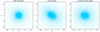 |
Fig. 7. Projected stellar particles of the main and remnant galaxies from a binary merger simulation. The left panel shows the initial main galaxy, while the middle and right panels show the uncircularized and circularized remnant galaxies, respectively. Length are in arbitrary units. |
The next step in generating mock observations is to assign physical units to the simulation data. In Nipoti et al. (2009b) code units were used for length. To compute Γ*, 10 for our mock galaxies, we first needed to specify a physical value for this length unit. We refer to this operation as rescaling the simulation data. To understand how mergers affect the growth of M*, 10 and Γ*, 10, we required a series of mock galaxies with different initial values of these parameters. This necessitated rescaling the simulation data several times to generate a series of mock galaxies. Setting the length unit to 1 kpc, the effective radius of the main galaxy is Re = 1.22 kpc, while Γ*, 10 ≈ 1.93. We then rescaled the simulation data, generating two additional sets of mock galaxies with effective radii Re = 8.5 kpc and Re = 11.5 kpc, with Γ*, 10 ≈ 1.50 and Γ*, 10 ≈ 1.44, respectively. These specific values were chosen to ensure the Γ*, 10 value of the rescaled mock galaxies fell within the gray band shown in Fig. 5, while maintaining moderate separation between them to facilitate the following analyses.
We then measured the evolution in log M*, 10 and Γ*, 10 for the mock galaxies. Fig. 8 shows the derivatives of log M*, 10 and Γ*, 10 with respect to log M* for three differently sized ETGs due to mergers, as a function of merger mass ratio ξ. Fig. 9 shows  versus
  for various ξ values. In both figures, each data point corresponds to one particular run of the simulations. The top row of Fig. 8 shows the log M* derivative of Γ*, 10 and illustrates that mergers always decrease Γ*, 10. The decrease can be explained by a scenario in which the stellar density profile is flattened by mergers, hence producing a shallower density slope. However, it is not straightforward to confirm this argument from the behavior of M*, 10, as its evolution due to mergers is somewhat complex and can be decomposed into two parts. The first part is induced by the increase in total stellar mass, while the second results from the change in density profile. Nevertheless, the signal of the first part can be approximated by homogeneous mass accretion, for which dlog M*, 10/dlog M* = 1. Therefore, the net effect of a merger on the density profile can be captured by dlog M*, 10/dlog M* − 1, as illustrated in the bottom row of Fig. 8. The negative value is evidence of a scenario in which the density profile is indeed flattened, as the mass of the inner region will outflow to the outer region during the flattening process, resulting in a decrease in M*, 10. A similar feature was also revealed in the work of Hilz et al. (2013), who performed N-body simulations of sequences of mergers, and showed that the slope of the stellar surface mass density profile becomes shallower after mergers (see their Figure 3).
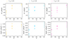 |
Fig. 8. Derivatives of log M*, 10 and Γ*, 10 with respect to log M* for three differently sized ETGs due to mergers. The first row shows the log M* derivative of Γ*, 10 for each merger mass ratio, ξ. The three columns correspond to different sets of mock galaxies with varying Γ*, 10. The second row shows the log M* derivative of log M*, 10, offset by one to remove the effect of homogeneous mass accretion. Each data point represents a particular run of simulations. For ξ = 1, two sets of simulations with two runs in each set are shown. For the other two values of ξ, three sets of simulations are shown. Note that in some cases two point overlap, hence the number of visible data points is smaller than the number of runs. |
We conclude that for the same amount of mass accreted via mergers, a smaller merger mass ratio ξ results in a flatter stellar density profile. Both dΓ*, 10/dlog M* and dlog M*, 10/dlog M* − 1 in Fig. 8 show a larger absolute value for lower ξ. In addition, for the same merger mass ratio ξ, the change in density profile is more significant for galaxies with larger Re and lower Γ*, 10, as shown in Fig. 9. The absolute value of  for galaxies with Γ*, 10 ≈ 1.93 is always smaller than for the other two sets of galaxies. In conclusion, mergers flatten the stellar density profile, with stronger flattening for lower ξ mergers.
 |
Fig. 9. Three panels illustrating changes in log M*, 10 and Γ*, 10 induced by mergers. Different colors represent distinct Γ*, 10 values of the main galaxy. Each data point corresponds to a particular run of simulations. For merger mass ratio ξ = 1, two sets of simulations with two runs in each set are shown. For the other two values of ξ, three sets of simulations are shown. Some data points overlap, hence the number of visible data points is smaller than the number of runs. |
4.2. Mass growth
The evolution of the Γ*, 10 − M*, 10 relation depends on the mass growth of ETGs. Leveraging binary merger simulations, we related the fractional mass growth, fM, to ζμ and ζβ within the redshift interval 0.17 ≤ z ≤ 0.37, specifically within the context of dry mergers.
As a first step, we considered a special condition in which all mass growth is induced by mergers of a single mass ratio ξ, focusing on ξ = 0.2, 0.5 and 1.0. To connect fM to ζμ and ζβ, we began by calculating the number of mergers, Nmerger, from the fractional mass growth, fM, then predicted the Γ*, 10 − M*, 10 relation after Nmerger merger events, and finally calculated the resulting ζμ and ζβ.
To calculate the number of merger events Nmerger in the first step, we simply divided fM by ξ:
 (28)
(28)
We note here that Nmerger does not describe individual galaxies, but represents an average for the entire galaxy population. Therefore, in principle, Nmerger can take any positive value, which can be used to predict the average evolution of M*, 10 and Γ*, 10 for the galaxy population in the following step.
The second step, predicting the Γ*, 10 − M*, 10 relation after Nmerger merger events, is more involved. First, we chose an initial Γ*, 10 − M*, 10 relation as the starting point. We set the starting Γ*, 10 − M*, 10 relation to be the median value of the gray band in Fig. 5. We located the initial state of mock galaxies with two rescaling settings, Γ*, 10 ≈ 1.50 and Γ*, 10 ≈ 1.41, on the starting Γ*, 10 − M*, 10 relation. The initial state of mock galaxies is shown in Fig. 10. The three different colors correspond to three different ξ mergers that the mock galaxies undergo. Due to different detailed settings in the simulation of those three ξ mergers (see Table 1 of Sonnenfeld et al. 2014), the positions of mock galaxies in Γ*, 10 − M*, 10 space exhibit slight offsets relative to one another. We then calculated the evolution of M*, 10 and Γ*, 10 for these two sets of rescaled galaxies in the context of three different ξ mergers, using the simulation results and Nmerger:
 (29)
(29)
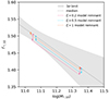 |
Fig. 10. Evolution of the Γ*, 10 − M*, 10 relation due to different merger toy models. As in Fig. 5, the gray band represents an upper limit of the evolution of the Γ*, 10 − M*, 10 relation. The median Γ*, 10 − M*, 10 relation of the gray band (shown as a dashed, gray line) serves as a starting point. The fitting formula of EMERGE (Moster et al. 2018) is used to estimate the number of mergers, thus calculating ζμ and ζβ. The three sets of dots that lie on the starting Γ*, 10 − M*, 10 relation represent three different merger models, while the arrows show the change of these dots and the resulting Γ*, 10 − M*, 10 relation. |
Here,  and
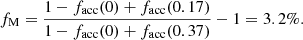
and  are the median values for each group of simulation data with different merger mass ratios for an entire merger event, as shown in Fig. 9. Adding the growth to the initial state yields the final state of our mock galaxies. Connecting the final states of the two groups of mock galaxies by dotted lines then gives the resulting Γ*, 10 − M*, 10 relation. Fig. 10 illustrates how the Γ*, 10 − M*, 10 relation evolves. In this figure, the values of ΔM*, 10 and ΔΓ*, 10 were calculated based on the fractional mass growth fM = 3.2% over z = 0.37 to z = 0.17 from Moster et al. (2018), which is further discussed in Sect. 5.1.
The third step involved calculating ζμ and ζβ. The change in normalization and slope was obtained by comparing the initial and resulting Γ*, 10 − M*, 10 relation given by the second step. By specifying a certain redshift interval, we then calculated the redshift derivatives of the normalization and slope of the Γ*, 10 − M*, 10 relation: ζμ and ζβ. For instance, applying this approach to the initial gray line and the three colored lines in Fig. 10, we obtained ζμ and ζβ for each ξ merger given fM in the redshift range 0.17 ≤ z ≤ 0.37 from Moster et al. (2018). The results are shown in Fig. 11 with star symbols for illustration.
 |
Fig. 11. Upper limit of Γ*, 10 − M*, 10 relation evolution in ζμ − ζβ space. The filled gray contour represents the estimate of the allowed evolution in the slope and normalization of the Γ*, 10 − M*, 10 relation. The star symbol indicates the prediction of ξ = 0.2 (in pink), ξ = 0.5 (in orange), and ξ = 1 (in blue) mergers, with merger numbers obtained from Moster et al. (2018). The arrows indicate the direction in which ζμ and ζβ would evolve if the number of merger events increases. We also include mass growth estimates, specifically |


To find a relation between fM and ζμ, ζβ in the redshift interval 0.17 ≤ z ≤ 0.37, we repeated the above three steps several times, with each iteration using a larger fractional mass growth fM. The three colored lines in Fig. 11 show how ζμ and ζβ evolve with fM, with arrows indicating the direction of increasing fM. The direction of each arrow depends on the merger mass ratio. All mergers decrease the normalization of the Γ*, 10 − M*, 10 relation, while the slope becomes steeper for ξ = 0.2 and ξ = 0.5 mergers but becomes shallower for ξ = 1.0 mergers.
We have now successfully connected ζμ and ζβ to fM in 0.17 ≤ z ≤ 0.37 under the condition that only mergers with a given merger mass ratio ξ contribute to the mass growth of ETGs. In reality, however, the mass growth is induced by a multitude of mergers involving different mass-ratio mergers. The total mass growth,  , is given by the sum of the mass growth, fM(ξ), induced by different ξ mergers:
 (30)
(30)
In this case, the first and second steps described above require modification. We calculated Nmerger(ξ) and thus obtained ΔM*, 10(ξ) and ΔΓ*, 10(ξ) for each ξ, summing ΔM*, 10(ξ) and ΔΓ*, 10(ξ) to get the total ΔM*, 10 and ΔΓ*, 10. Hence, a precise fM(ξ) is required to find the precise relation between  and ζμ, ζβ. The different directions of the three arrows in Fig. 11 suggest that if ζμ and ζβ can be measured precisely, we might infer the fractional mass growth, fM(ξ), for different ξ mergers. However, our observations are currently limited by systematics, and thus not sufficiently precise to infer fM(ξ).
Nevertheless, our initial goal, which was to explore to what extent the evolution of the Γ*, 10 − M*, 10 relation in redshift range 0.17 ≤ z ≤ 0.37 can be explained by dry mergers, can still be achieved. This is possible because mergers with smaller mass ratios ξ cause a more significant evolution in Γ*, 10 − M*, 10 relation, which is reflected by the three star symbols in Fig. 11. The three symbols have the same fractional mass growth, but the ζμ and ζβ values of the ξ = 0.2 merger are the largest. In other words, mergers with larger ξ must induce more mass growth of ETGs to achieve the same degree of evolution in the Γ*, 10 − M*, 10 relation as mergers with smaller ξ values. Therefore, we can use the largest ξ, which is ξ = 1, to place an upper limit on the fractional mass growth fM. Using the toy model for single mass ratio ξ = 1 mergers, the maximum fractional mass growth fM in the redshift range 0.17 < z < 0.37 is found to be 11.2%. This represents the fM boundary where the dry merger scenario is viable. If the fractional mass growth fM of ETGs in the redshift range 0.17 ≤ z ≤ 0.37 is less than 11.2%, or Δlog M*/Δt ≤ 0.022 dex/Gyr, then the dry merger scenario is consistent with our observational limits on the evolution of the Γ*, 10 − M*, 10 relation.
5. Discussion
5.1. Comparison with the literature
Our observations do not show evidence for evolution of the Γ*, 10 − M*, 10 relation. This is qualitatively consistent with Huang et al. (2018), whose Figure 6 shows that the inner mass profile of massive galaxies in the redshift range 0.25 ≤ z ≤ 0.50 are similar to those of z ∼ 0 massive galaxies.
We compared our upper limit on the fractional mass growth with results from the literature. We first compared fM with an empirical model, EMERGE (Moster et al. 2018). This is a semi-analytic model designed to populate mock galaxies inside simulated dark matter halos, thereby providing predictions for galaxy formation and evolution. For EMERGE, we obtained the fractional mass growth fM in the redshift range 0.17 ≤ z ≤ 0.37 from the fraction of stellar mass accreted to the main galaxy as a function of redshift, facc, with respect to z = 0. This is given by Eq. (24) in Moster et al. (2018):
![Mathematical equation: $$ \begin{aligned} f_{\rm acc}(z) = 0.55\exp \left[-1.09(z+1)\right]. \end{aligned} $$](/articles/aa/full_html/2025/09/aa53788-25/aa53788-25-eq49.gif) (31)
(31)
Hence, fM can be calculated by substituting the lower and upper redshifts of our sample:
 (32)
(32)
This value is smaller than the maximum allowed fractional mass growth fM = 11.2% obtained from our toy model. We further checked the induced ζμ and ζβ, using the procedure introduced in Sect. 4.2 for three different ξ mergers. The three star symbols in Fig. 11, representing the resulting positions in ζμ − ζβ space, all lie within the gray contour. Therefore, we consider the EMERGE result consistent with our observation.
Next, we compared our results with the observation of Conselice et al. (2022), who defined major mergers as those with mass ratio ξ ≥ 0.25 and minor mergers as those with mass ratio 0.1 ≤ ξ ≤ 0.25. They selected galaxies from the REFINE survey in the redshift range 0 < z < 3 and separated them into different redshift bins, then measured the number of merger events in each redshift bin and inferred the amount of accreted mass as a function of redshift. For comparison, we selected the redshift bin 0.2 < z < 0.5, as it is the closest to our redshift range 0.17 ≤ z ≤ 0.37. According to Conselice et al. (2022), the stellar mass of the main galaxies, which later merge with their nearby lower-mass companions, is log M* = 11.3 ± 0.1 in this redshift bin, and the mass accreted via major and minor mergers is  and
and  , respectively (see Table 2 in Conselice et al. 2022). Assuming a constant accretion rate during 0.2 < z < 0.5, we calculated the total accreted mass
  in our focused redshift range 0.17 ≤ z ≤ 0.37, then calculated the fractional mass growth
  . We then applied the ξ = 0.2 merger scenario to evolve the Γ*, 10 − M*, 10 relation according to
  , and the ξ = 1 merger scenario to evolve the Γ*, 10 − M*, 10 relation according to
  . The outcome is plotted in Fig. 11 as the green point, with the error bar representing the uncertainty. The green point lies inside the gray contour, indicating that the result of Conselice et al. (2022) is also consistent with our observations.
Although the fractional mass growths predicted by EMERGE and Conselice et al. (2022) observations are similar, the induced ζμ and ζβ differ, as shown in Fig. 11. We believe that the potential remains to distinguish different merger scenarios, provided sufficiently precise measurement. To measure ζμ and ζβ precisely, we need to overcome the limitation imposed by systematics. The pink star symbol in Fig. 11 shows the induced ζμ and ζβ of the fM predicted by the EMERGE model. Although this symbol correspond to the most extreme case in which all mergers have the smallest mass ratio ξ = 0.2, it still lies inside the gray contour, which indicates that the systematics in the data may be larger than the intrinsic evolution of the Γ*, 10 − M*, 10 relation. We therefore discuss the possible sources of systematics in the following Sect. 5.2.
Nevertheless, we believe that applying our method to a larger redshift baseline could potentially detect a real signal of evolution in the Γ*, 10 − M*, 10 relation, thereby achieving a better understanding of the late growth of ETGs. To provide a rough estimate, we utilized the ζμ and ζβ derived from the result of Conselice et al. (2022). We find that if we explore to a higher redshift of z = 0.54, i.e., a time interval Δt = 3.2 Gyr, the Γ*, 10 − M*, 10 relation will evolve outside the gray contour. Hence, we believe that focusing on a redshift range with a time interval longer than Δt ≥ 3.2 Gyr, will allow the signal of evolution in the Γ*, 10 − M*, 10 relation to emerge above the systematics.
5.2. Possible source of systematics
In our observations, we adopted a conservative approach, leading to the identification of the gray band that serves as the upper limit of the evolution of the Γ*, 10 − M*, 10 relation. The Γ*, 10 − M*, 10 relation could have evolved its slope and normalization in the redshift range 0.17 ≤ z ≤ 0.37, but must be constrained within the gray band. We suspect that quantities that were derived from photometry could be affected by systematics, although we lack robust methods to quantitatively estimate and eliminate them.
One possible source of bias is the stellar population synthesis model on which the measurement of the stellar mass-to-light ratio of our galaxies are based. Stellar population synthesis fits to broadband imaging data are prone to systematic errors (see e.g. Conroy 2013), which may be redshift-dependent. For instance, Paulino-Afonso et al. (2022) found that the stellar masses of z = 0.5 galaxies are underestimated by 0.1 − 0.2 dex, compared to their z = 0 counterparts. Nevertheless, we suspect that such biases are highly dependent on the details of the stellar population modeling methods and data used; therefore, we refrain from applying a correction to our results based on their analysis.
Another potential source of systematics is the presence of color gradients. Galaxies are typically bluer in their outer regions (e.g. Suess et al. 2019a,b, 2020), making them appear more extended when observed at shorter wavelengths. We compared our observations with those of Cannarozzo et al. (2020), computing M*, 10 and Γ*, 10 for 63 overlapping galaxies from their Sérsic model fits. We find discrepancies between the two datasets, as shown in Fig. 12. Both log M*, 10 and Γ*, 10 are systematically smaller in our sample than in Cannarozzo et al. (2020), with median discrepancies of 0.1 dex and 0.04, respectively. The depths of both surveys are sufficient to capture the full extent of galaxy light within a radius of 10 kpc. For our highest-redshift subsample (0.39 < z < 0.40), the typical surface brightness at 10 kpc is approximately 24 mag/arcsec2. This is well above the detection threshold of the shallower KiDS survey, which is typically 26 mag/arcsec2, as measured from galaxies shown in Fig. 1. Therefore, the main difference between these two measurements is that they use observed data at different wavelength ranges. Cannarozzo et al. (2020) use g, r, i, z, and y-band Hyper Suprime-Cam(HSC) Subaru Strategic Program(SSP) data, with the i-band data having the best S/N. Hence, we believe that the i-band plays the major role in determining the stellar mass and the surface brightness profile. In contrast, we used data in a fixed wavelength range 3000 − 10 000 Å to measure the stellar mass and only the r-band, which has a shorter wavelength than the i-band, to measure the Sérsic parameters. The discrepancy in Γ*, 10 measurement can be qualitatively explained by the existence of the color gradient, as the smaller values of Γ*, 10 in our sample are consistent with the trend that galaxies appear more extended in bluer filter bands. Our choice to ignore the color gradient in our sample therefore introduces a potential systematic bias in the measurements of M*, 10 and Γ*, 10.
 |
Fig. 12. Differences in the derived M*, 10 (top panel) and Γ*, 10 (bottom panel) using different Sérsic parameters (Re and n). The superscripts ‘this work’ and ‘Can20’ indicate that Re and n are taken from this work and from Cannarozzo et al. (2020), respectively. The dashed line represents the median value of the difference. |
This bias could be alleviated by obtaining spatially resolved stellar population synthesis models, although at the expense of a significant increase in the complexity of our analysis. We defer such efforts to future work.
Finally, another important systematic effect is progenitor bias (Dokkum & Franx 1996; Saglia et al. 2010; Carollo et al. 2013; Fagioli et al. 2016). The population of quiescent galaxies is continuously augmented by the addition of recently quenched ex-star-forming galaxies, which in turn leaves imprints on the average Γ*, 10 − M*, 10 relation. One solution to remove this bias could be to trace the evolutionary tracks for both star-forming and quiescent galaxies. Progenitor bias does not necessarily affect our measurements, but it complicates their interpretation. To account for progenitor bias, we would need to analyze star-forming galaxies in addition to ETGs. However, the transition from star-forming to quiescent galaxies changes their morphology in a nontrivial way, making it unclear how to map objects from one population to the other. Moreover, comparing stellar mass measurements of galaxy populations with very different star formation histories can be subject to bias. Another possible solution is to focus on ETGs only and trace the descendants of higher redshift ETGs using proxies, for instance, the Dn4000 index (Zahid et al. 2019; Hamadouche et al. 2022; Damjanov et al. 2023). In principle, we can use stellar population synthesis models to predict the evolution of the Dn4000 index of quiescent galaxies, and a redshift-dependent Dn4000 cut can be applied to follow galaxies along their evolutionary tracks. However, further investigation is required to validate the robustness of this approach with respect to choices of the underlying stellar population synthesis model. We therefore leave this analysis to future work.
6. Conclusion
In this work, we provide a new perspective on investigating the evolution of quiescent galaxies. Instead of attempting to obtain information on stellar mass and effective radius from the entire light of a galaxy, we focused our attention to the inner region. In particular, we focused on a fixed physical aperture of 10 kpc and measured the stellar mass and the stellar mass-weighted projected surface brightness slope Γ*, 10 enclosed within this aperture, known as the 10 kpc collar.
First, combining KiDS imaging with GAMA spectroscopy, we measured the Γ*, 10 − M*, 10 relation in four different redshift bins with a Bayesian hierarchical model, while correcting for the Eddington bias. Due to potential uncertainties and systematic effects, current observations are not sufficient to detect an evolution in the Γ*, 10 − M*, 10 relation. We placed an upper limit on the parameters ζμ and ζβ, which are the redshift derivatives of the normalization and slope of the Γ*, 10 − M*, 10 relation. The values of the upper limits are |ζμ|≤0.13 and |ζβ| ≤ 1.10.
For interpretation of these observations, we focused on dissipationless mergers, a well-agreed mechanism driving the growth of galaxies. To understand how mergers evolve quiescent galaxies in Γ*, 10 − M*, 10 space, we utilized a collection of dissipationless binary merger simulations. We analyzed the difference between pre-merger mock galaxies and post-merger galaxies and draw the following conclusions:
-
Mergers flatten the density profile and thus result in a decrease in Γ*, 10. This is reflected by the fact that all post-merger mock galaxies have a smaller Γ*, 10 compared with their pre-merger counterparts. The larger decrease in Γ*, 10 for lower ξ mergers indicates that the flattening is stronger for smaller mass-ratio mergers.
-
In most cases, mergers induce an increase in M*, 10. However, M*, 10 decreases when galaxies with low Γ*, 10 undergo low-ξ mergers. This indicates that the effect of minor mergers is to redistribute stellar mass toward the outer regions.
After characterizing how mergers evolve galaxies in the M*, 10 − Γ*, 10 space, we established a toy model to explore to what extent a dry merger scenario can explain the possible evolution of the Γ*, 10 − M*, 10 relation. We find that the effect of mergers on the Γ*, 10 − M*, 10 relation depends on the merger mass ratio. The normalization of the Γ*, 10 − M*, 10 relation always decreases after mergers, while the slope of the Γ*, 10 − M*, 10 relation becomes either shallower or steeper, depending on the merger mass ratio. We then used the upper limit on ζμ and ζβ to find the maximum fractional mass growth fM = 11.2% of ETGs during 0.17 ≤ z ≤ 0.37, below which the dry merger scenario remains consistent with our observations. We compared our maximum fM with the empirical model EMERGE Moster et al. (2018) and the observations of Conselice et al. (2022), finding consistency with both.
Furthermore, we discussed the possible source of bias and systematics in our observations. We find that measurement of both M*, 10 and Γ*, 10 depend on the wavelength used in the analysis, which suggests that color gradients in galaxies should not be ignored. Another potential source of bias could be the contamination from newly quenched star-forming galaxies. In the presence of these systematics, a larger redshift baseline, particularly Δz ≥ 0.45, may be needed to observe a signal of evolution in the Γ*, 10 − M*, 10 relation. Further efforts are needed to either extend the redshift baseline or eliminate the possible systematics, thereby improving our understanding of the post-quenching evolution of ETGs.
In conclusion, we present a new method to investigate the evolution of quiescent galaxies, establishing a toy model based on N-body simulations to predict the impact of different mergers on the Γ*, 10 − M*, 10 relation. When applied to data from the GAMA survey, our method is currently limited by systematics in the stellar mass estimate. However, upcoming surveys such as Euclid (Euclid Collaboration: Scaramella et al. 2022) and CSST (Zhan 2021) are expected to expand coverage and deepen survey-limiting fluxes. We believe that these improvements will help overcome the current limitation and enable more precise conclusions on the evolution of quiescent galaxies in the near future.
Acknowledgments
This work was supported by the National Key R&D Program of C’hina (No. 2023YFA1607800, 2023YFA1607802), and made use of the Gravity Supercomputer at the Department of Astronomy, Shanghai Jiao Tong University.
References
- Auger, M. W., Treu, T., Bolton, A. S., et al. 2010, ApJ, 724, 511 [NASA ADS] [CrossRef] [Google Scholar]
- Baldry, I. K., Robotham, A. S. G., Hill, D. T., et al. 2010, MNRAS, 404, 86 [NASA ADS] [Google Scholar]
- Balogh, M. L., Morris, S. L., Yee, H. K. C., Carlberg, R. G., & Ellingson, E. 1999, ApJ, 527, 54 [Google Scholar]
- Belli, S., Newman, A. B., & Ellis, R. S. 2015, ApJ, 799, 206 [NASA ADS] [CrossRef] [Google Scholar]
- Bellstedt, S., Driver, S. P., Robotham, A. S. G., et al. 2020, MNRAS, 496, 3235 [NASA ADS] [CrossRef] [Google Scholar]
- Bruzual, G., & Charlot, S. 2003, MNRAS, 344, 1000 [NASA ADS] [CrossRef] [Google Scholar]
- Bundy, K., Leauthaud, A., Saito, S., et al. 2017, ApJ, 851, 34 [Google Scholar]
- Calzetti, D., Armus, L., Bohlin, R. C., et al. 2000, ApJ, 533, 682 [NASA ADS] [CrossRef] [Google Scholar]
- Cannarozzo, C., Sonnenfeld, A., & Nipoti, C. 2020, MNRAS, 498, 1101 [NASA ADS] [CrossRef] [Google Scholar]
- Carollo, C. M., Bschorr, T. J., Renzini, A., et al. 2013, ApJ, 773, 112 [NASA ADS] [CrossRef] [Google Scholar]
- Chabrier, G. 2003, PASP, 115, 763 [Google Scholar]
- Chen, X., Zu, Y., Shao, Z., & Shan, H. 2022, MNRAS, 514, 2692 [NASA ADS] [CrossRef] [Google Scholar]
- Conroy, C. 2013, ARA&A, 51, 393 [NASA ADS] [CrossRef] [Google Scholar]
- Conselice, C. J., Mundy, C. J., Ferreira, L., & Duncan, K. 2022, ApJ, 940, 168 [CrossRef] [Google Scholar]
- Daddi, E., Renzini, A., Pirzkal, N., et al. 2005, ApJ, 626, 680 [NASA ADS] [CrossRef] [Google Scholar]
- Damjanov, I., Zahid, H. J., Geller, M. J., et al. 2019, ApJ, 872, 91 [NASA ADS] [CrossRef] [Google Scholar]
- Damjanov, I., Sohn, J., Geller, M. J., Utsumi, Y., & Dell’Antonio, I. 2023, ApJ, 943, 149 [NASA ADS] [CrossRef] [Google Scholar]
- de Jong, J. T. A., Kuijken, K., Applegate, D., et al. 2013, The Messenger, 154, 44 [NASA ADS] [Google Scholar]
- Dehnen, W. 1993, MNRAS, 265, 250 [NASA ADS] [CrossRef] [Google Scholar]
- Dekel, A., & Burkert, A. 2014, MNRAS, 438, 1870 [Google Scholar]
- D’Eugenio, F., van der Wel, A., Piotrowska, J. M., et al. 2023, MNRAS, 525, 2789 [CrossRef] [Google Scholar]
- Dokkum, P. G. V., & Franx, M. 1996, MNRAS, 281, 985 [NASA ADS] [CrossRef] [Google Scholar]
- Driver, S. P., Bellstedt, S., Robotham, A. S. G., et al. 2022, MNRAS, 513, 439 [NASA ADS] [CrossRef] [Google Scholar]
- D’Souza, R., Kauffman, G., Wang, J., & Vegetti, S. 2014, MNRAS, 443, 1433 [Google Scholar]
- Eisenstein, D. J., Willott, C., Alberts, S., et al. 2023, ArXiv e-prints [arXiv:2306.02465] [Google Scholar]
- Euclid Collaboration (Scaramella, R., et al.) 2022, A&A, 662, A112 [NASA ADS] [CrossRef] [EDP Sciences] [Google Scholar]
- Fagioli, M., Carollo, C. M., Renzini, A., et al. 2016, ApJ, 831, 173 [NASA ADS] [CrossRef] [Google Scholar]
- Fan, L., Lapi, A., De Zotti, G., & Danese, L. 2008, ApJ, 689, L101 [NASA ADS] [CrossRef] [Google Scholar]
- Gardner, J. P., Mather, J. C., Abbott, R., et al. 2023, PASP, 135, 068001 [NASA ADS] [CrossRef] [Google Scholar]
- Hamadouche, M. L., Carnall, A. C., McLure, R. J., et al. 2022, MNRAS, 512, 1262 [NASA ADS] [CrossRef] [Google Scholar]
- Hilz, M., Naab, T., & Ostriker, J. P. 2013, MNRAS, 429, 2924 [NASA ADS] [CrossRef] [Google Scholar]
- Hopkins, P. F., Hernquist, L., Cox, T. J., Keres, D., & Wuyts, S. 2009, ApJ, 691, 1424 [Google Scholar]
- Hopkins, P. F., Bundy, K., Hernquist, L., Wuyts, S., & Cox, T. J. 2010, MNRAS, 401, 1099 [NASA ADS] [CrossRef] [Google Scholar]
- Hopkins, A. M., Driver, S. P., Brough, S., et al. 2013, MNRAS, 430, 2047 [NASA ADS] [CrossRef] [Google Scholar]
- Huang, S., Leauthaud, A., Greene, J. E., et al. 2018, MNRAS, 475, 3348 [Google Scholar]
- Huang, S., Leauthaud, A., Hearin, A., et al. 2020, MNRAS, 492, 3685 [NASA ADS] [CrossRef] [Google Scholar]
- Kauffmann, G., Heckman, T. M., White, S. D. M., et al. 2003, MNRAS, 341, 33 [Google Scholar]
- Kawinwanichakij, L., Papovich, C., Ciardullo, R., et al. 2020, ApJ, 892, 7 [Google Scholar]
- Kuijken, K., Heymans, C., Dvornik, A., et al. 2019, A&A, 625, A2 [NASA ADS] [CrossRef] [EDP Sciences] [Google Scholar]
- Li, R., Napolitano, N. R., Roy, N., et al. 2022, ApJ, 929, 152 [NASA ADS] [CrossRef] [Google Scholar]
- Moster, B. P., Naab, T., & White, S. D. M. 2018, MNRAS, 477, 1822 [Google Scholar]
- Naab, T., Johansson, P. H., & Ostriker, J. P. 2009, ApJ, 699, L178 [Google Scholar]
- Navarro, J. F., Frenk, C. S., & White, S. D. M. 1996, ApJ, 462, 563 [Google Scholar]
- Newman, A. B., Ellis, R. S., Bundy, K., & Treu, T. 2012, ApJ, 746, 162 [NASA ADS] [CrossRef] [Google Scholar]
- Nipoti, C. 2025, A&A, 697, A74 [NASA ADS] [CrossRef] [EDP Sciences] [Google Scholar]
- Nipoti, C., Treu, T., Auger, M. W., & Bolton, A. S. 2009a, ApJ, 706, L86 [NASA ADS] [CrossRef] [Google Scholar]
- Nipoti, C., Treu, T., & Bolton, A. S. 2009b, ApJ, 703, 1531 [Google Scholar]
- Nipoti, C., Treu, T., Leauthaud, A., et al. 2012, MNRAS, 422, 1714 [NASA ADS] [CrossRef] [Google Scholar]
- Oser, L., Naab, T., Ostriker, J. P., & Johansson, P. H. 2011, ApJ, 744, 63 [Google Scholar]
- Paulino-Afonso, A., González-Gaitán, S., Galbany, L., et al. 2022, A&A, 662, A86 [NASA ADS] [CrossRef] [EDP Sciences] [Google Scholar]
- Roy, N., Napolitano, N. R., La Barbera, F., et al. 2018, MNRAS, 480, 1057 [Google Scholar]
- Saglia, R. P., Sánchez-Blázquez, P., Bender, R., et al. 2010, A&A, 524, A6 [NASA ADS] [CrossRef] [EDP Sciences] [Google Scholar]
- Sersic, J. L. 1968, Atlas de Galaxias Australes [Google Scholar]
- Sonnenfeld, A. 2020, A&A, 641, A143 [NASA ADS] [CrossRef] [EDP Sciences] [Google Scholar]
- Sonnenfeld, A., Nipoti, C., & Treu, T. 2014, ApJ, 786, 89 [NASA ADS] [CrossRef] [Google Scholar]
- Spavone, M., Krajnović, D., Emsellem, E., Iodice, E., & den Brok, M. 2021, A&A, 649, A161 [NASA ADS] [CrossRef] [EDP Sciences] [Google Scholar]
- Suess, K. A., Kriek, M., Price, S. H., & Barro, G. 2019a, ApJ, 877, 103 [NASA ADS] [CrossRef] [Google Scholar]
- Suess, K. A., Kriek, M., Price, S. H., & Barro, G. 2019b, ApJ, 885, L22 [NASA ADS] [CrossRef] [Google Scholar]
- Suess, K. A., Kriek, M., Price, S. H., & Barro, G. 2020, ApJ, 899, L26 [Google Scholar]
- Suess, K. A., Williams, C. C., Robertson, B., et al. 2023, ApJ, 956, L42 [CrossRef] [Google Scholar]
- Tal, T., & van Dokkum, P. G. 2011, ApJ, 731, 89 [NASA ADS] [CrossRef] [Google Scholar]
- Taylor, E. N., Hopkins, A. M., Baldry, I. K., et al. 2011, MNRAS, 418, 1587 [Google Scholar]
- Toft, S., van Dokkum, P., Franx, M., et al. 2007, ApJ, 671, 285 [CrossRef] [Google Scholar]
- Tremaine, S., Richstone, D. O., Byun, Y.-I., et al. 1994, AJ, 107, 634 [CrossRef] [Google Scholar]
- Trujillo, I., Feulner, G., Goranova, Y., et al. 2006, MNRAS, 373, L36 [NASA ADS] [CrossRef] [Google Scholar]
- Trujillo, I., Conselice, C. J., Bundy, K., et al. 2007, MNRAS, 382, 109 [NASA ADS] [CrossRef] [Google Scholar]
- van der Wel, A., Franx, M., van Dokkum, P. G., et al. 2014, ApJ, 788, 28 [Google Scholar]
- van Dokkum, P. G., & Brammer, G. 2010, ApJ, 718, L73 [NASA ADS] [CrossRef] [Google Scholar]
- van Dokkum, P. G., & Franx, M. 2001, ApJ, 553, 90 [NASA ADS] [CrossRef] [Google Scholar]
- van Dokkum, P. G., Franx, M., Kriek, M., et al. 2008, ApJ, 677, L5 [Google Scholar]
- van Dokkum, P. G., Whitaker, K. E., Brammer, G., et al. 2010, ApJ, 709, 1018 [Google Scholar]
- Williams, D. J., Damjanov, I., Sawicki, M., et al. 2025, ApJ, 989, 107 [Google Scholar]
- Zahid, H. J., Geller, M. J., Damjanov, I., & Sohn, J. 2019, ApJ, 878, 158 [Google Scholar]
- Zhan, H. 2021, Chin. Sci. Bull., 66, 1290 [CrossRef] [Google Scholar]
All Tables
Median values of the marginal posterior probability of the model parameters in each redshift bin.
All Figures
|
Fig. 1. Surface brightness profile of 25 galaxies. These galaxies were selected after visually inspecting 69 galaxies in one KiDS tile and randomly choosing 25 from the 62 without bright companions. The upper panel shows the surface brightness as a function of the circularized radius. The solid blue line shows the best-fitting Sérsic model convolved with PSF, calculated using GalNet structural parameters. The blue diamonds show measurements directly obtained from the KiDS r-band image. The lower panel shows the difference between the two measurements. The vertical dashed pink line indicates the angular size corresponding to 10 kpc for each galaxy. The horizontal line represents the noise level of the sky. |
| In the text | |
|
Fig. 2. Distribution of M*, 10/F in three narrow redshift bins. The vertical dashed line marks the 95th percentile of the distribution in each bin. By multiplying this ratio by the flux corresponding to the r-band magnitude limit, rcrit = 19.65, we obtain the M*, 10 limit for that redshift bin. |
| In the text | |
|
Fig. 3. Distribution of our galaxy sample in z − M*, 10 space (top) and z − M* space (bottom). The 95% completeness M*, 10 limit as a function of redshift of our ETG sample is shown by the solid pink line. Galaxies above this pink line, shown as black dots, are included in our complete sample; gray dots below the line are excluded. We further define lower and upper redshift limits of z ≥ 0.15 and z ≤ 0.40, respectively, to build the final sample shown as blue dots. |
| In the text | |
|
Fig. 4. Distribution of our 5690 ETGs in M*, 10, Γ*, 10, and redshift z. |
| In the text | |
|
Fig. 5. The Γ*, 10 − M*, 10 relation of our observation sample fitted using a Bayesian hierarchical model. For each redshift bin, the median value of this relation is shown as a dotted line, while the shaded region represents the 68% credible interval. The gray region indicates the estimated 3 − σ systematic uncertainty. |
| In the text | |
|
Fig. 6. Posterior distributions of the hyperparameters in the Bayesian hierarchical model corresponding to the Γ*, 10 − M*, 10 relation. The contours represent the 68% and 95% credible interval. |
| In the text | |
|
Fig. 7. Projected stellar particles of the main and remnant galaxies from a binary merger simulation. The left panel shows the initial main galaxy, while the middle and right panels show the uncircularized and circularized remnant galaxies, respectively. Length are in arbitrary units. |
| In the text | |
|
Fig. 8. Derivatives of log M*, 10 and Γ*, 10 with respect to log M* for three differently sized ETGs due to mergers. The first row shows the log M* derivative of Γ*, 10 for each merger mass ratio, ξ. The three columns correspond to different sets of mock galaxies with varying Γ*, 10. The second row shows the log M* derivative of log M*, 10, offset by one to remove the effect of homogeneous mass accretion. Each data point represents a particular run of simulations. For ξ = 1, two sets of simulations with two runs in each set are shown. For the other two values of ξ, three sets of simulations are shown. Note that in some cases two point overlap, hence the number of visible data points is smaller than the number of runs. |
| In the text | |
|
Fig. 9. Three panels illustrating changes in log M*, 10 and Γ*, 10 induced by mergers. Different colors represent distinct Γ*, 10 values of the main galaxy. Each data point corresponds to a particular run of simulations. For merger mass ratio ξ = 1, two sets of simulations with two runs in each set are shown. For the other two values of ξ, three sets of simulations are shown. Some data points overlap, hence the number of visible data points is smaller than the number of runs. |
| In the text | |
|
Fig. 10. Evolution of the Γ*, 10 − M*, 10 relation due to different merger toy models. As in Fig. 5, the gray band represents an upper limit of the evolution of the Γ*, 10 − M*, 10 relation. The median Γ*, 10 − M*, 10 relation of the gray band (shown as a dashed, gray line) serves as a starting point. The fitting formula of EMERGE (Moster et al. 2018) is used to estimate the number of mergers, thus calculating ζμ and ζβ. The three sets of dots that lie on the starting Γ*, 10 − M*, 10 relation represent three different merger models, while the arrows show the change of these dots and the resulting Γ*, 10 − M*, 10 relation. |
| In the text | |
|
Fig. 11. Upper limit of Γ*, 10 − M*, 10 relation evolution in ζμ − ζβ space. The filled gray contour represents the estimate of the allowed evolution in the slope and normalization of the Γ*, 10 − M*, 10 relation. The star symbol indicates the prediction of ξ = 0.2 (in pink), ξ = 0.5 (in orange), and ξ = 1 (in blue) mergers, with merger numbers obtained from Moster et al. (2018). The arrows indicate the direction in which ζμ and ζβ would evolve if the number of merger events increases. We also include mass growth estimates, specifically |
| In the text | |
|
Fig. 12. Differences in the derived M*, 10 (top panel) and Γ*, 10 (bottom panel) using different Sérsic parameters (Re and n). The superscripts ‘this work’ and ‘Can20’ indicate that Re and n are taken from this work and from Cannarozzo et al. (2020), respectively. The dashed line represents the median value of the difference. |
| In the text | |
Current usage metrics show cumulative count of Article Views (full-text article views including HTML views, PDF and ePub downloads, according to the available data) and Abstracts Views on Vision4Press platform.
Data correspond to usage on the plateform after 2015. The current usage metrics is available 48-96 hours after online publication and is updated daily on week days.
Initial download of the metrics may take a while.