| Issue |
A&A
Volume 701, September 2025
|
|
|---|---|---|
| Article Number | A240 | |
| Number of page(s) | 22 | |
| Section | Planets, planetary systems, and small bodies | |
| DOI | https://doi.org/10.1051/0004-6361/202554040 | |
| Published online | 22 September 2025 | |
The CHEOPS view of HD 95338b: Refined transit parameters, and a search for exomoons★
1
Konkoly Observatory, HUN-REN Research Centre for Astronomy and Earth Sciences,
Konkoly Thege út 15–17.,
1121
Budapest,
Hungary
2
CSFK, MTA Centre of Excellence, Budapest,
Konkoly Thege út 15–17.,
1121
Budapest,
Hungary
3
HUN-REN-ELTE Exoplanet Research Group,
Szent Imre h. u. 112.,
Szombathely
9700,
Hungary
4
ELTE Eötvös Loránd University, Doctoral School of Physics,
Budapest,
H-1117 Budapest Pázmány Péter sétány 1/A,
Hungary
5
Center for Space and Habitability, University of Bern,
Gesellschaftsstrasse 6,
3012
Bern,
Switzerland
6
Observatoire astronomique de l’Université de Genève,
Chemin Pegasi 51,
1290
Versoix,
Switzerland
7
Institute of Space Research, German Aerospace Center (DLR),
Rutherfordstrasse 2,
12489
Berlin,
Germany
8
ELTE Gothard Astrophysical Observatory,
9700
Szombathely,
Szent Imre h. u. 112,
Hungary
9
Centre Vie dans l’Univers, Faculté des sciences, Université de Genève,
Quai Ernest-Ansermet 30,
1211
Genève 4,
Switzerland
10
Department of Physics, University of Warwick,
Gibbet Hill Road,
Coventry
CV4 7AL,
UK
11
European Space Agency (ESA), European Space Research and Technology Centre (ESTEC),
Keplerlaan 1,
2201
AZ
Noordwijk,
The Netherlands
12
Instituto de Astrofisica e Ciencias do Espaco, Universidade do Porto, CAUP, Rua das Estrelas,
4150-762
Porto,
Portugal
13
Space sciences, Technologies and Astrophysics Research (STAR) Institute, Université de Liège,
Allée du 6 Août 19C,
4000
Liège,
Belgium
14
Space Research Institute, Austrian Academy of Sciences,
Schmiedlstrasse 6,
8042
Graz,
Austria
15
INAF, Osservatorio Astrofisico di Catania,
Via S. Sofia 78,
95123
Catania,
Italy
16
Department of Astronomy, Stockholm University, AlbaNova University Center,
10691
Stockholm,
Sweden
17
Instituto de Astrofísica de Canarias, Vía Láctea s/n,
38200
La Laguna, Tenerife,
Spain
18
Departamento de Astrofísica, Universidad de La Laguna, Astrofísico Francisco Sanchez s/n,
38206
La Laguna, Tenerife,
Spain
19
Admatis,
5. Kandó Kálmán Street,
3534
Miskolc,
Hungary
20
Depto. de Astrofísica, Centro de Astrobiología (CSIC-INTA), ESAC campus,
28692
Villanueva de la Cañada (Madrid),
Spain
21
Departamento de Fisica e Astronomia, Faculdade de Ciencias, Universidade do Porto, Rua do Campo Alegre,
4169-007
Porto,
Portugal
22
Max Planck Institute for Extraterrestrial Physics,
Gießenbachstraße 1,
Garching bei München
85748,
Germany
23
INAF, Osservatorio Astronomico di Padova,
Vicolo dell’Osservatorio 5,
35122
Padova,
Italy
24
Centre for Exoplanet Science, SUPA School of Physics and Astronomy, University of St Andrews,
North Haugh,
St Andrews
KY16 9SS,
UK
25
CFisUC, Departamento de Física, Universidade de Coimbra,
3004-516
Coimbra,
Portugal
26
INAF, Osservatorio Astrofisico di Torino,
Via Osservatorio, 20,
10025
Pino Torinese To,
Italy
27
Centre for Mathematical Sciences, Lund University,
Box 118,
221 00
Lund,
Sweden
28
Aix Marseille Univ, CNRS, CNES, LAM,
38 rue Frédéric Joliot-Curie,
13388
Marseille,
France
29
SRON Netherlands Institute for Space Research,
Niels Bohrweg 4,
2333
CA
Leiden,
The Netherlands
30
Leiden Observatory, University of Leiden,
PO Box 9513,
2300
RA
Leiden,
The Netherlands
31
Department of Space, Earth and Environment, Chalmers University of Technology, Onsala Space Observatory,
439 92
Onsala,
Sweden
32
Dipartimento di Fisica, Università degli Studi di Torino,
via Pietro Giuria 1,
10125
Torino,
Italy
33
National and Kapodistrian University of Athens, Department of Physics, University Campus, Zografos
157 84,
Athens,
Greece
34
Astrobiology Research Unit, Université de Liège,
Allée du 6 Août 19C,
4000
Liège,
Belgium
35
Department of Astrophysics, University of Vienna,
Türkenschanzstrasse 17,
1180
Vienna,
Austria
36
Division Technique INSU, CS20330,
83507
La Seyne sur Mer cedex,
France
37
Institute for Theoretical Physics and Computational Physics, Graz University of Technology,
Petersgasse 16,
8010
Graz,
Austria
38
ELTE Eötvös Loránd University, Institute of Physics,
Pázmány Péter sétány 1/A,
1117
Budapest,
Hungary
39
IMCCE, UMR8028 CNRS, Observatoire de Paris, PSL Univ., Sorbonne Univ.,
77 av. Denfert-Rochereau,
75014
Paris,
France
40
Institut d’astrophysique de Paris, UMR7095 CNRS, Université Pierre & Marie Curie,
98bis blvd. Arago,
75014
Paris,
France
41
Astrophysics Group, Lennard Jones Building, Keele University,
Staffordshire
ST5 5BG,
UK
42
European Space Agency, ESA – European Space Astronomy Centre, Camino Bajo del Castillo s/n,
28692
Villanueva de la Cañada, Madrid,
Spain
43
Weltraumforschung und Planetologie, Physikalisches Institut, University of Bern,
Gesellschaftsstrasse 6,
3012
Bern,
Switzerland
44
Dipartimento di Fisica e Astronomia “Galileo Galilei”, Università degli Studi di Padova,
Vicolo dell’Osservatorio 3,
35122
Padova,
Italy
45
ETH Zurich, Department of Physics,
Wolfgang-Pauli-Strasse 2,
8093
Zurich,
Switzerland
46
Cavendish Laboratory,
JJ Thomson Avenue,
Cambridge
CB3 0HE,
UK
47
Fachbereich Geowissenschaften, Freie Universität Berlin, Institut für Geologische Wissenschaften, Fachrichtung Planetologie und Fernerkundung,
Malteserstr. 74–100,
12249
Berlin,
Germany
48
Institut de Ciencies de l’Espai (ICE, CSIC), Campus UAB, Can Magrans s/n,
08193
Bellaterra,
Spain
49
Institut d’Estudis Espacials de Catalunya (IEEC),
08860
Castelldefels (Barcelona),
Spain
50
Institute of Astronomy, University of Cambridge,
Madingley Road,
Cambridge
CB3 0HA,
UK
51
Deutsches Zentrum für Luft- und Raumfahrt (DLR),
Markgrafenstrasse 37,
10117
Berlin,
Germany
52
Université de Paris, Institut de physique du globe de Paris, CNRS,
75005
Paris,
France
53
Laboratory for Climate and Ocean-Atmosphere Studies, Department of Atmospheric and Oceanic Sciences, School of Physics, Peking University,
Beijing
100871,
China
★★ Corresponding author.
Received:
5
February
2025
Accepted:
15
July
2025
Abstract
Context. Despite the ever-increasing number of known exoplanets, no uncontested detections have been made of their satellites, known as exomoons.
Aims. The quest to find exomoons is at the forefront of exoplanetary sciences. Certain space-born instruments are thought to be suitable for this purpose. We show the progress made with the CHaracterising ExOPlanets Satellite (CHEOPS) in this field using the HD 95338 planetary system. We present a novel methodology as an important step in the quest to find exomoons.
Methods. We utilised ground-based spectroscopic data in combination with Gaia observations to obtain precise stellar parameters. These were then used as input in the analysis of the planetary transits observed by CHEOPS and the Transiting Exoplanet Survey Satellite (TESS). In addition, we searched for the signs of satellites primarily in the form of additional transits in the Hill sphere of the eccentric Neptune-sized planet HD 95338b in a sequential approach based on four CHEOPS visits. We also briefly explored the transit timing variations of the planet.
Results. We present refined stellar and planetary parameters, narrowing down the uncertainty on the planet-to-star radius ratio by a factor of ten. We also pin down the ephemeris of HD 95338b. Using injection-and-retrieval tests, we show that a 5σ detection of an exomoon would be possible at RMoon = 0.8 R⊕ with the methodology presented here.
Conclusions. We exclude the transit of an exomoon in the HD 95338 system with RMoon ≈0.6 R⊕ at the 1σ level. The algorithm used for finding the transit-like event can be used as a baseline for other similar targets, observed by CHEOPS or other missions.
Key words: methods: data analysis / techniques: photometric / planets and satellites: individual: HD 95338b
Based on data from CHEOPS Guaranteed Time Observations, collected under Programme ID CH_PR100009 and CH_PR140072.
© The Authors 2025
 Open Access article, published by EDP Sciences, under the terms of the Creative Commons Attribution License (https://creativecommons.org/licenses/by/4.0), which permits unrestricted use, distribution, and reproduction in any medium, provided the original work is properly cited.
This article is published in open access under the Subscribe to Open model. This email address is being protected from spambots. You need JavaScript enabled to view it. to support open access publication.
1 Introduction
Following the discovery of the first confirmed extrasolar planet orbiting a main sequence star (Mayor & Queloz 1995), close to 6000 exoplanets have been identified1. One of the key points of these past decades is the fact that the Solar system is not unique in many aspects: it is simply one of the ever-growing number of known planetary systems in our Galaxy. Based on our understanding of the Solar System, we expect that there are perhaps orders of magnitude more satellites orbiting exoplanets compared to the number of exoplanets. Yet at the time of writing, there are no confirmed exomoons, but there are a number of possible explanations for this (see Szabó et al. 2024, and references therein). With the introduction of space telescopes such as Kepler (Borucki et al. 2010) and CHaracterising ExOPlanets Satellite (CHEOPS; Benz et al. 2021), we have the theoretical capability of finding transiting exomoons below the size of Earth.
The Kepler space telescope was the first instrument recognised to be able to detect an exomoon (Szabó et al. 2006; Simon et al. 2007). Kipping et al. (2015) and Kipping et al. (2022) performed extensive analyses of Kepler light curves with the aim of finding transiting exomoons, yielding Kepler-1708b-i as a candidate. Another method thought to be useful for detection of satellites is based on the transit timing tariations (TTVs) of the planets (Simon et al. 2007; Kipping 2009) caused by exomoons. Fox & Wiegert (2021) identified six candidates based on their Kepler datasets, which were found to be false positives by Kipping (2020). Kipping & Yahalomi (2023) found no strong TTV signals that could be linked to satellites in a large set of suitable planets observed by Kepler. Simon et al. (2015) predicted that Earth-sized exomoons could likely be detectable with CHEOPS. For that reason, a considerable effort has been devoted within the CHEOPS Science Team to observing systems that are likely to sustain exomoons for long periods of time (see e.g. Dobos et al. 2022) in pursuit of detecting these objects. Ehrenreich et al. (2023) found that there are likely no transiting bodies above the size of Mars orbiting ν2 Lupi d, based on 1.5 transits observed with CHEOPS.
In this paper, we present the necessary steps in the search for moons orbiting the bright (V = 8.62 mag) star HD 95338, including refining the stellar and planetary parameters, analysing synthetic data, and placing upper limits on the hypothesised satellite. Díaz et al. (2020) reported the discovery of a dense Neptune-sized planet (![Mathematical equation: $\[3.89_{-0.20}^{+0.19}\]$](/articles/aa/full_html/2025/09/aa54040-25/aa54040-25-eq1.png) R⊕,
R⊕, ![Mathematical equation: $\[42.44_{-2.08}^{+2.22}\]$](/articles/aa/full_html/2025/09/aa54040-25/aa54040-25-eq2.png) M⊕, yielding a density of
M⊕, yielding a density of ![Mathematical equation: $\[3.98_{-0.64}^{+0.62}\]$](/articles/aa/full_html/2025/09/aa54040-25/aa54040-25-eq3.png) g cm−3), HD 95338b. Based on a single transit observed by the Transiting Exoplanet Survey Satellite (TESS; Ricker et al. 2015) and a large number of radial velocity measurements, Díaz et al. (2020) found an orbital period of 55.087 ± 0.020 days. This meant that the planet could be far enough from its host star that an exomoon could survive for several gigayears (Dobos et al. 2022), yet close enough that it can be observed multiple times during the life cycle of CHEOPS, leading to tighter constraints on its parameters, as well as on those of its hypothetical companion. However, due to the Sun-synchronous, dusk-dawn low Earth orbit of the satellite, long-period planets might only be observable once a year.
g cm−3), HD 95338b. Based on a single transit observed by the Transiting Exoplanet Survey Satellite (TESS; Ricker et al. 2015) and a large number of radial velocity measurements, Díaz et al. (2020) found an orbital period of 55.087 ± 0.020 days. This meant that the planet could be far enough from its host star that an exomoon could survive for several gigayears (Dobos et al. 2022), yet close enough that it can be observed multiple times during the life cycle of CHEOPS, leading to tighter constraints on its parameters, as well as on those of its hypothetical companion. However, due to the Sun-synchronous, dusk-dawn low Earth orbit of the satellite, long-period planets might only be observable once a year.
This paper is structured as follows. In Sect. 2, we describe in detail the photometry of CHEOPS and TESS observations, with a special emphasis on the various detrending steps needed to account for the known instrumental effects. We also provide details of the modelling of the transit of HD 95338b. New and improved stellar parameters are provided in Sect. 3. In Sect. 4, we present the refined planetary parameters, based on five transits observed with CHEOPS and TESS. In Sect. 5, we present a novel method for chasing transits linked to exomoons. We argue for the need of a thorough noise treatment to avoid false positive exomoon detections. We exclude the presence of Mars-sized transiting exomoons at 1σ. In Sect. 5.3, we present the analyses of synthetic data, which are used to justify the algorithm utilised in the search for additional transits. We show that even from a single transit, the 3σ detection of a less than 1 R⊕ transit would be feasible in this system.
2 Methods
2.1 CHEOPS photometry
CHEOPS observed four transits of HD 95338b (during four separate visits) in March 2021, April 2022, May 2023, and April 2025 (Table A.1). The spacecraft is on a low Earth orbit, with an ≈100 min period. Consequently, targets cannot be observed continuously throughout an orbit due to Earth occultations, crossing over the South Atlantic Anomaly, and too high stray-light contributions, as is often discussed with regards to CHEOPS data (e.g. Lacedelli et al. 2022; Krenn et al. 2024). This is reflected in the so-called observational efficiency (Table A.1). We extracted light curves using the CHEOPS Data Reduction Pipeline (DRP; version 14.1.2; Hoyer et al. 2020). The DRP performs the bias, read-out noise, flatfield, and smearing-corrections, while also estimating the telescope jitter and background contamination. The pipeline also carries out aperture photometry using a circular apertures, with radii between 15 and 40 pixels (in 1-pixel steps). In this work, we rely on light curves extracted using the R = 25 px radius aperture (the so-called default mode).
Due to the spacecraft rolling around its line of sight, the well-known triangular point spread function (as discussed in e.g. Szabó et al. 2021; Kiefer et al. 2023) of any given star (Fig. 1) falls onto different pixels throughout each orbit (causing a part of the flux to fall in and out of the circular aperture as the telescope rolls). Several factors, including the inhomogeneous nature of the CCD, stray light, smearing trails, and thermal variability of the instrument result in the appearance of periodic or quasi-periodic systematic effects that are correlated with the angular orientation (and possibly the jitter) of the spacecraft. Additionally, the flux contribution of nearby stars also introduces a noise source that changes throughout each orbit and is therefore correlated in nature. The background variation thus also has to be estimated for every exposure.
We emphasise, that in the context of nominal science observations, a subset of the full frame images, known as ‘window images’, are downlinked. In order to minimise the noise caused by bad pixels, it is necessary to move the position of the window in the CCD to different regions of the CCD when required. In May 2024, the position of the window was relocated to the central location of the CCD2. This resulted in the fourth visit being observed in a distinct region of the CCD compared to the initial three observations. This modification has resulted in a shift in the configuration of the star pattern within the full frame. This alteration has had an impact on the correlation between the flux and the roll angle of the telescopes (and the number of used harmonics of the roll angle in the analysis). This is due to the fact that the smearing trails of the background stars within the full frame intersect the window as the field rotates around the target star.
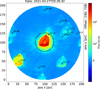 |
Fig. 1 The Subarray image depicts the point spread function (PSF) of HD 95338b and the neighbouring stars, with their respective magnitudes of brightness indicated. The target is centred on the coordinates (180, 178) on the CCD. |
2.2 TESS photometry
In addition to the CHEOPS photometry described above, we also obtained the short-cadence SAP (Simple Aperture Photometry) light curves from sectors 10 and 63 of TESS (Transiting Exoplanet Survey Satellite; Ricker et al. 2015). These include one transit of HD 95338b each. The transit from sector 10 was also analysed by Díaz et al. (2020). We corrected for contamination in the aperture using the CROWDSAP keyword. We downloaded the light curves from the two sectors from MAST. Additionally, we corrected for the pointing instability of the telescope using the pipeline-estimated position of the photocenter. As a final preparatory step, we cut out a 1.5 and a 3-day window (in sectors 10 and 63, respectively) of the light curves – that are centered on the two transits – in order to minimise the computational time needed for the analysis described below.
2.3 Modelling the transit of HD 95338b from CHEOPS
There are a number of algorithms and software packages capable of modelling a transiting exoplanet and their satellites, including planetplanet (Luger et al. 2017), the phase-folding method by Kipping (2021), the analytical framework of Saha & Sengupta (2022), and Pandora (Hippke & Heller 2022). There are, however, none that incorporate the advanced noise filtering algorithms such as those based on Gaussian processes (GPs; e.g. Rasmussen & Williams 2006; Roberts et al. 2012; Ebden 2015) or a wavelet-based technique (e.g. Carter & Winn 2009). These tools are used to deal with the time-correlated noise arising from both astrophysical and instrumental noise sources. Their benefits in avoiding distortions of the light curve parameters of transiting exoplanets are clearly demonstrated in Barros et al. (2020), Csizmadia et al. (2023), and Kálmán et al. (2023b). Regarding the detection of exomoon transits specifically, Kálmán et al. (2024a) and Szabó et al. (2024) discuss the implications of insufficient noise treatment.
The two perhaps most well-known exomoon candidates, Kepler-1625b-i (Teachey & Kipping 2018) and Kepler-1708b-i (Kipping et al. 2022), identified by a so-called photodynamical method, where the parameters of the planet and its satellite are fitted jointly, are not confirmed through independent investigations. In fact, Heller et al. (2019) and Kreidberg et al. (2019) provide alternative explanation for the exomoon signal observed in Kepler-1625b-i, involving the presence of red noise. More recently, Heller & Hippke (2024) presented evidence suggesting that ‘large exomoons are unlikely’ around both Kepler-1625b and Kepler-1708b, although this is again refuted (Kipping et al. 2025). It is reasonable to expect that a simultaneous fitting of the planetary and lunar signals with the time-correlated noise would be beneficial in discerning false-positives from bona fide exomoons.
Lacking such a tool, we developed a sequential scheme to search for exomoon-like signals in the CHEOPS light curves of HD 95338b. In the first step, we model the transit of HD 95338b, then in the second step, we search the residuals for signs of additional transits. The transit signal that could be attributed to an exomoon has an amplitude on the order of ≈100 ppm (as is discussed in Section 5). Thus a thorough detrending of the known systematic effects is essential to avoid false-positive detections. We therefore constructed a strict framework to handle the known (quasi-periodic) systematic effects as follows:
- 0.
Remove light curve points that are heavily affected by cosmic rays and remove four points before and after each gap (only for the fourth visit).
- 1.
Conduct preliminary transit modelling of HD 95338b.
- 2.
Find the best-fit model of the instrumental effects in the residuals of the previous step; find the >3σ outliers in the residuals of this step.
- 3.
Subtract the best-fit systematics model from the raw light curve and mask the outliers identified in the previous step.
- 4.
Model the transit of HD 95338b in the pre-whitened light curve.
- 5.
Check the residuals for transits of an exomoon.
In step 2, we constructed a basis vector (FBV) for detrending (following the common recipe, e.g. Szabó et al. 2021; Smith & Csizmadia 2022) in the form of
![Mathematical equation: $\[F_{\mathrm{BV}, N}=\sum_{i=1}^N\left(a_i ~\sin~ (i \phi)+b_i ~\cos~ (i \phi)\right),\]$](/articles/aa/full_html/2025/09/aa54040-25/aa54040-25-eq4.png) (1)
(1)
where ϕ is the roll angle of the spacecraft, ai and bi are amplitudes of the sinusoidal terms. We then used the Bayesian Information Criterion (BIC Schwarz 1978) to find the optimal number of harmonics N, where N ∈ {1 . . . 10}, to be included in the detrending process. Defining the optimal set of detrending vectors is also part of the optimisation problem, and besides the roll angle harmonics, all telemetry data and by-products of the photometry reduction pipeline have initially been considered. We concluded that the background contamination is among the most important detrending parameters, and therefore, we included this vector into the noise model as well.
We analysed the transits of HD 95338b using the Transit and Light Curve Modeller (TLCM; Csizmadia 2020). TLCM uses a two-dimensional Gauss-Legendre integration approach to calculate the transit curves. These are described in terms of the scaled semi-major axis of the planet, a/R⋆, the planet-to-star radius ratio, Rp/R⋆, the time of mid-transit, T0, and the orbital period, P. Díaz et al. (2020) found that the planet has an eccentric orbit, specifically, an eccentricity of e = 0.127 ± 0.045 and an argument of the periastron ω = 39.4° ± 18.7°. In TLCM, it is possible to account for the orbital eccentricity, where the ingress and egress durations can differ. In that case, instead of the commonly used impact parameter, the so-called (inferior) conjunction parameter contains the information of the orbital inclination of the planet (i). It is given by Csizmadia (2020) as:
![Mathematical equation: $\[b^{\prime}=\frac{a}{R_{\star}} \frac{\left(1-e^2\right) ~\cos~ i}{(1+e ~\sin~ \omega)}.\]$](/articles/aa/full_html/2025/09/aa54040-25/aa54040-25-eq5.png) (2)
(2)
We fixed e and ω at their reported values during the light curve modelling.
Stellar limb darkening is taken into account via the quadratic law (Wade & Rucinski 1985), described by the linear (u1) and quadratic (u2) coefficients using the re-parametrisation introduced in Kálmán et al. (2024b) and Harre et al. (2024):
![Mathematical equation: $\[A=\frac{1}{4}\left(u_1\left(\frac{1}{\alpha}-\frac{1}{\beta}\right)+u_2\left(\frac{1}{\alpha}+\frac{1}{\beta}\right)\right),\]$](/articles/aa/full_html/2025/09/aa54040-25/aa54040-25-eq6.png) (3)
(3)
![Mathematical equation: $\[B=\frac{1}{4}\left(u_1\left(\frac{1}{\alpha}+\frac{1}{\beta}\right)+u_2\left(\frac{1}{\alpha}-\frac{1}{\beta}\right)\right),\]$](/articles/aa/full_html/2025/09/aa54040-25/aa54040-25-eq7.png) (4)
(4)
where ![Mathematical equation: $\[\alpha=\frac{1}{2} ~\cos~ \left(77^{\circ}\right)\]$](/articles/aa/full_html/2025/09/aa54040-25/aa54040-25-eq8.png) , and
, and ![Mathematical equation: $\[\beta=\frac{1}{2} ~\sin~ \left(77^{\circ}\right)\]$](/articles/aa/full_html/2025/09/aa54040-25/aa54040-25-eq9.png) . In step 1 of the algorithm, the A and B parameters were fitted using the [1.06, 1.56] and [1.40, 1.80] uniform priors, respectively. These priors are set according to the theoretical limb-darkening of the star (with stellar parameters from Table 1), as calculated by LDCU3. This software uses a modified version of the routines of Espinoza & Jordán (2015) to calculated the limb darkening coefficients, based on stellar intensity profiles calculated via the ATLAS (Kurucz 1979) and PHOENIX (Husser et al. 2013) models. In step 4, when the definitive planetary parameters are computed, the A and B coefficients were treated as free parameters of the fit.
. In step 1 of the algorithm, the A and B parameters were fitted using the [1.06, 1.56] and [1.40, 1.80] uniform priors, respectively. These priors are set according to the theoretical limb-darkening of the star (with stellar parameters from Table 1), as calculated by LDCU3. This software uses a modified version of the routines of Espinoza & Jordán (2015) to calculated the limb darkening coefficients, based on stellar intensity profiles calculated via the ATLAS (Kurucz 1979) and PHOENIX (Husser et al. 2013) models. In step 4, when the definitive planetary parameters are computed, the A and B coefficients were treated as free parameters of the fit.
Furthermore, TLCM uses the wavelet-based formalism of Carter & Winn (2009) to handle time-correlated noise (also commonly known as ‘red noise’) that comprises of any remaining instrumental effects or astrophysical variations (Csizmadia et al. 2023). This technique introduces two additional fitting parameters, σw for the standard deviation of the white noise component and σr for characterising the red component. These are fitted simultaneously with the parameters describing the transits. To avoid overcorrecting the light curves, the red noise fit is constrained by prescribing that the standard deviation of the white noise (i.e. the residuals) has to be equal to the mean photometric uncertainty of the input light curve (Csizmadia et al. 2023). In step 1, this technique is used to handle the instrumental noise sources, as the wavelet-based noise model is fitted jointly with the transits. Theoretical limb darkening coefficients are needed at this phase to retrieve plausible transit shapes. This allows for a clear detection of the instrument-related effects in step 2. The wavelet-based noise handling is used again in step 4 to obtain the final set of planetary parameters. At this stage, it is expected that astrophysical noise sources will make up the majority of the autocorrelated effects. We emphasise that, from the perspective of the planetary transit fitting, any additional transits – including those from an exomoon – are treated as noise by the wavelet technique or other non-parametric methods, and were therefore removed. For this reason, the search for moons needs to occur on a residual light curve where the time-correlated effects (that are not clearly attributed to instrumental effects) are not removed. Therefore, the complex detrending process outlined above is warranted.
A much less computationally efficient method would be to fit the FBV jointly with the (planetary) transits and the wavelet-based noise model4. This would, however, involve the introduction of up to 66 additional fitting parameters, since the ai and bi coefficients of Eq. (1), as well as the amplitudes of the background contamination are independent variables in the four visits. In the steps outlined above, the systematic effects are fitted using a simple least squares method, which is several orders of magnitude faster than the joint FBV plus red noise plus transit fit in our experience. This way, we are able to drastically narrow down the parameter space of the transit modelling itself, thus reducing the possibilities for the MCMC chains to get stuck in so-called local minima, and increasing the reliability of the solutions.
Stellar parameters of HD 95338.
2.4 Joint TESS+CHEOPS modelling
In order to increase the precision of the recovered planetary parameters, we also performed a joint TESS+CHEOPS LC analysis. We assume that the passband-independent orbital parameters, including the eccentricity, the argument of periastron, the semi-major axis and the orbital period remain constant on the timescale relevant in these observations. We also assume that although the TESS passband is redder compared to CHEOPS (see e.g. Scandariato et al. 2024), the possible atmospheric features on HD 95338b are not detectable with the present noise levels, meaning that there is no wavelength-dependence of the transit depth. Therefore, we assumed that Rp/R⋆ is the same in the two passbands. We further assumed that the transit chord does not change between the different observations, meaning that the scaled semi-major axis, the conjunction parameter, and the orbital period are the same for all five modelled transits. The limb-darkening coefficients are passband-dependent, which neccesitates the inclusion of ACHEOPS, BCHEOPS, ATESS, and BTESS into the analysis. It is understood that red noise from an astrophysical origin decreases with increasing wavelength. This manifests in an expectedly lower σr (see e.g. Kálmán et al. 2023a) in the TESS observations compared to the CHEOPS light curves. On the other hand, the white noise level depends primarily on the aperture size and the exposure time. We therefore include ![Mathematical equation: $\[\sigma_{r}^{\text {CHEOPS}}, ~\sigma_{w}^{\text {CHEOPS}}, ~\sigma_{r}^{\text {TESS}}\]$](/articles/aa/full_html/2025/09/aa54040-25/aa54040-25-eq12.png) , and
, and ![Mathematical equation: $\[\sigma_{w}^{\text {TESS}}\]$](/articles/aa/full_html/2025/09/aa54040-25/aa54040-25-eq13.png) in the global LC modelling. The likelihood of the joint TESS+CHEOPS modelling is then the sum of the log-likelihoods of the light curve fits of the data from the two satellites.
in the global LC modelling. The likelihood of the joint TESS+CHEOPS modelling is then the sum of the log-likelihoods of the light curve fits of the data from the two satellites.
In addition to increasing the number of transits that can be analysed, the two different passbands also allowed us to break the degeneracy between the limb-darkening coefficients and the transit parameters, yielding more precise estimates on both.
During the revision of this paper, Saha (2025) published an independent analysis based on the first three transits from CHEOPS and the two TESS transits.
2.5 Sampling the posterior distributions
In every TLCM-based light curve analysis described in this paper, we followed the same recipe. We used wide, uninformed priors on every parameter. A genetic algorithm is then able to find the (global) minimum in the likelihood space, with Ninit = 2000 randomly selected values for each parameter (see Csizmadia 2020, for more details). Having found starting points that are suspected to be good, we applied a Differential Evolution Markov-chain Monte Carlo (DE-MCMC; Ter Braak 2006) to get robust estimates of the uncertainty ranges of the fitting parameters. In every case, we used ten chains (also known as walkers) each consisting of 20 000 possible steps. The convergence was monitored via the Gelman–Rubin statistic (Gelman & Rubin 1992) and the effective sample size (e.g. Ripley 1987). If convergence is not reached within these 20 000 steps, the chain length is automatically extended to 10 · 20 000.
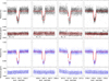 |
Fig. 2 Demonstration of the fitting and detrending steps. The raw CHEOPS light curves of HD 95338b are shown in the top row, along with the initially fitted transit curves (step 1). The residuals of the initial transit fit, along with the best-fit systematics model is shown in the second row, with N number of harmonics of the roll angle included. The final transit fit (step 4) and its residuals (later used in the search for additional transits) are shown in the bottom two rows, where the full white circles represent 200-point bins (with an average uncertainty of ≈20 ppm in each bin). |
3 Stellar parameters
We used the ARES+MOOG spectroscopic analysis methodology to derive the stellar spectroscopic parameters (Teff, log g, micro-turbulence, [Fe/H]). This methodology is described in detail in Sousa et al. (2021); Sousa (2014); Santos et al. (2013). The equivalent widths (EW) were consistently measured using the ARES code5 (Sousa et al. 2007, 2015). We used the list of iron lines appropriate for stars cooler that 5200 K which was presented in Tsantaki et al. (2013). For this spectral analysis we used a combined HARPS spectrum of HD 95338. To converge for the best set of spectroscopic parameters for each spectrum we use a minimisation process to find the ionisation and excitation equilibrium. This process makes use of a grid of Kurucz model atmospheres (Kurucz 1993) and the latest version of the radiative transfer code MOOG (Sneden 1973). We also derived a more accurate trigonometric surface gravity using recent Gaia data following the same procedure as described in Sousa et al. (2021) which provided a consistent value (4.44 ± 0.04 dex) when compared with the spectroscopic surface gravity.
We computed the stellar radius of HD 95338 utilising a MCMC modified infrared flux method (IRFM – Blackwell & Shallis 1977; Schanche et al. 2020) that allows us to produce synthetic photometry from a constructed spectral energy distribution (SED) using stellar atmospheric models (Castelli & Kurucz 2003) and our stellar spectroscopic parameters as priors. These simulated data are compared to broadband fluxes in the following bandpasses: Gaia G, GBP, and GRP, 2MASS J, H, and K, and WISE W1 and W2 (Skrutskie et al. 2006; Wright et al. 2010; Gaia Collaboration 2023) that are listed in Table 4 of Díaz et al. (2020) to derive the stellar bolometric flux. The last step in the MCMC is to convert this flux to the stellar effective temperature and angular diameter, that is combined with the offset-corrected Gaia parallax (Lindegren et al. 2021) to produce the stellar radius.
To accurately characterise the stellar properties of HD 95338 and account for some modelling systematics, we derived two pairs of {M⋆, t⋆} from two different approaches. The first mass and age pair were estimated by applying the isochrone placement algorithm (Bonfanti et al. 2015, 2016) that interpolates the input stellar parameters within pre-computed grids of isochrones and tracks of PARSEC6 v1.2S (Marigo et al. 2017). The second pair of mass and age estimates were derived from a Levenberg-Marquardt minimisation scheme (as detailed in Salmon et al. 2021) computing stellar models on the fly with the CLÉS code (Code Liégeois d’Évolution Stellaire – Scuflaire et al. 2008). This minimisation scheme optimises over the age and mass to produce the best agreement between model and observed radii and effective temperatures. As detailed in Bonfanti et al. (2021), we checked the mutual consistency between the two respective pairs of outcomes via a χ2-based criterion and then merged the results obtaining M⋆ = 0.848 ± 0.043 M⊙ and t⋆ = ![Mathematical equation: $\[9.5_{-5.7}^{+4.3}\]$](/articles/aa/full_html/2025/09/aa54040-25/aa54040-25-eq14.png) Gyr.
Gyr.
The derived stellar parameters are listed in Table 1. In general, they are in good agreements with the values reported by Díaz et al. (2020), although we present more precise estimates on R⋆ and log g, which are used in the transit modelling.
In order to increase the precision and accuracy of the planetary model, we incorporated the stellar parameters of Table 1 as inputs to the light curve analysis. By a rearrangement of Kepler’s third law of planetary motion, the scaled semi-major axis is connected to the stellar density as well, since (under the assumption of a spherical star)
![Mathematical equation: $\[\left(\frac{a}{R_{\star}}\right)^3=P^2 G(1+q) \frac{\rho_{\star, \text {transit}}}{3 \pi},\]$](/articles/aa/full_html/2025/09/aa54040-25/aa54040-25-eq25.png) (5)
(5)
where q = Mp/M⋆, and ρ⋆,transit is a geometrically constrained density, since a/R⋆ is determined from the transit duration. Using the estimated Teff, [Fe/H] and ρ⋆,ransit, we are able to provide estimate M⋆,transit and R⋆,transit using the empirical formulae7 of Southworth (2011). Then, according to Csizmadia (2020), the goodnes-of-fit metric (in this case, the logarithmic likelihood) can be modified as
![Mathematical equation: $\[\begin{aligned}-\log \mathcal{L}_{\text {mod }}= & -\log \mathcal{L}+\frac{1}{2}\left(\frac{R_{\star}-R_{\star, \text {transit }}}{\sqrt{\left(\Delta R_{\star}\right)^2+\left(\Delta R_{\star, \text {transit}}\right)^2}}\right)^2 \\& +\frac{1}{2}\left(\frac{\log g-\left.\log g\right|_{\text {transit }}}{\sqrt{(\Delta \log g)^2+\left(\left.\Delta \log g\right|_{\text {transit }}\right)^2}}\right)^2,\end{aligned}\]$](/articles/aa/full_html/2025/09/aa54040-25/aa54040-25-eq26.png) (6)
(6)
where log g|transit = 4.43–2 log R⋆,transit + log M⋆,transit, where log g⊙ = 4.43. Given that both the second and third terms contain information about ρtransit, a/R⋆ is constrained via the input stellar parameters as well.
Parameters obtained from the transit modelling of HD 95338b.
4 Results
4.1 Planetary parameters
The best-fit CHEOPS and TESS light curves (from the joint fit) are shown in Figs. 3 and 4. The corresponding parameters are shown in Table 2. The parameters describing the planetary transit agree well with each other between the CHEOPS only and the joint TESS plus CHEOPS modelling. We note that the uncertainty ranges do not decrease with the inclusion of the two additional TESS transits, which implies that they are dominated by the uncertainty in the input stellar parameters. The best-fit conjunction parameter is in a <1σ agreement with the impact parameter presented by Díaz et al. (2020), and the relative planetary radius shows a discrepancy of only ≈1.2σ. There is a 4.8σ disagreement between the estimated a/R⋆ values, and a 2.8σ difference between the T0 from our joint TESS+CHEOPS analysis and the respective values shown by Díaz et al. (2020). Using the S/N criteria established by Csizmadia et al. (2023) for a/R⋆, we know that from the CHEOPS analysis alone, we are able to constrain the scaled semi-major axis well within 2% of the truth (since for a 2% accuracy, a S/N = 3 is needed, and in our case, S/N = 22). Consequently, we argue that the uncertainty range presented in Díaz et al. (2020) is likely underestimated. Díaz et al. (2020) find that the first TESS transits occurs 166 ± 52 seconds earlier than our estimates, which is likely a combination of inadequate noise treatment (Kiefer et al. 2023) and the fact that we analyse five transits together. However, the discrepancy in T0 is <3σ. A brief TTV (transit timing variation) analysis is shown in Sect. 4.2.
The smaller aperture of the TESS cameras implies that the TESS observations are more noisy – this is confirmed by the higher ![Mathematical equation: $\[\sigma_{w}^{\text {TESS}}\]$](/articles/aa/full_html/2025/09/aa54040-25/aa54040-25-eq27.png) compared to
compared to ![Mathematical equation: $\[\sigma_{w}^{\text {CHEOPS}}\]$](/articles/aa/full_html/2025/09/aa54040-25/aa54040-25-eq28.png) . The red noise parameters are not directly comparable between the two instruments, although we expect the this noise type to decrease at longer wavelengths (e.g. Kálmán et al. 2023a). The retrieved ACHEOPS and BCHEOPS are within 3σ of the theoretical values. Both limb darkening coefficients in the TESS passband are in agreement with those presented by Díaz et al. (2020) (after conversion to the formalism used in this paper).
. The red noise parameters are not directly comparable between the two instruments, although we expect the this noise type to decrease at longer wavelengths (e.g. Kálmán et al. 2023a). The retrieved ACHEOPS and BCHEOPS are within 3σ of the theoretical values. Both limb darkening coefficients in the TESS passband are in agreement with those presented by Díaz et al. (2020) (after conversion to the formalism used in this paper).
Our results are also in agreement with the parameters presented by Saha (2025). Due to the additional transit included in this work and the refined stellar parameters, we estimate slightly lower uncertainties in Rp/R⋆, b′, P, and T0. A direct comparison of the confidence intervals of a/R⋆ and the limb-darkening coefficients is not applicable, since Saha (2025) did not use these as fitting parameters.
We find that the planetary orbit has an inclination of 89.654° ± 0.0155°, the planet has a radius of Rp = 0.3811 ± 0.0035RJup, with a transit duration of ![Mathematical equation: $\[5.587_{-0.016}^{+0.018}\]$](/articles/aa/full_html/2025/09/aa54040-25/aa54040-25-eq29.png) hours.
hours.
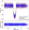 |
Fig. 3 Phase-folded detrended CHEOPS light curve of HD 95338 (top panel, orange; same data as the third row of Fig. 2.) The rednoise-corrected light curve is shown with blue, while the best-fit transit light curves of HD 95338b is represented by the solid red curve. |
 |
Fig. 4 Phase-folded detrended TESS light curve of HD 95338 (top panel, orange, the same data as the third row of Fig. 2.) The rednoise-corrected light curve is shown with blue, while the best-fit transit light curves of HD 95338b is represented by the solid red curve. |
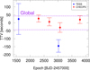 |
Fig. 5 Transit timing data of HD 95338b. The dashed purple lines represent the uncertainty range from the global fit. |
4.2 Transit timing
We extracted the timing of each individual transit (two from TESS, four from CHEOPS) by fixing all parameters to the best-fit values from Table 2 with the exception of σw, σr and T0, assuming a constant orbital period. We also included a possible quadratic trend in the modellings. The resultant transit timing data are shown in Fig. 5 and are compiled in Table 3. There is no apparent TTV, meaning that the transit timings are explained well by a constant period. The T0 value from sector 63 is in a 2.5σ disagreement with the global modelling, which is not statistically significant. A deeper exploration of the TTV signals is beyond the scope of this paper.
5 The search for moons
We chose to restrict the search for exomoons on the CHEOPS dataset alone. This is done because the smaller (mirror) aperture of TESS in comparison to CHEOPS manifests as higher white noise levels, which are detrimental to the quest for moons with the methodology presented here (191 ppm for CHEOPS compared to 289 ppm in TESS despite the exposure time that is more than 4 times shorter, Table 2). For that reason, and to keep the analysis self-consistent, we use the planetary orbital parameters (P, b and a/R⋆) that are derived from the CHEOPS photometry alone in the processes described below.
5.1 Sensitivity maps
We examined the CHEOPS residual light curves for shallow transit signals (that could be linked to an exomoon) following the approach detailed in Ehrenreich et al. (2023). This method explores a grid of moon transit epochs and durations {T0,Moon, W}. For each point of the grid, we fit for a box-shaped transit depth (allowed to be negative) together with a trend (linear or quadratic) and a multiplicative noise term (factor applied to the data error bars). The fit is done using the Markov chain Monte Carlo algorithm (MCMC) implemented in the Python package emcee (Foreman-Mackey et al. 2013). From the posterior distribution on the transit depth, we derive the best-fit value of the moon radius and its 3-σ lower limit. We also compute the Bayesian Information Criterion and the Akaike Information Criteria (AIC; Akaike 1998) defined as:
![Mathematical equation: $\[\mathrm{BIC}=k ~\ln (n)-2 ~\ln (\mathcal{L})\]$](/articles/aa/full_html/2025/09/aa54040-25/aa54040-25-eq30.png) (7)
(7)
![Mathematical equation: $\[\mathrm{AIC}=2 k-2 ~\ln (\mathcal{L}),\]$](/articles/aa/full_html/2025/09/aa54040-25/aa54040-25-eq31.png) (8)
(8)
where n is the number of data points, k is the number of parameters included in the fit, ℒ is the best-fit (maximum) likelihood value. The BIC and AIC values are compared to their respective values in the case where the moon transit depth is fixed to 0, i.e. a ‘no-moon’ reference fit.
The parameter space scanned by the {T0,Moon, W} grid must cover mid-transit times across the full Hill-sphere of HD 95338b8 while allowing for either shorter or longer transit duration (e.g. if the moon impact parameter is larger or smaller) than that of its planet. With a transit duration of the Hill sphere of 17.6 ± 0.9 hours (i.e. <20.3 h at 3 σ), we considered T0,Moon values that satisfy −10.5 h ≤ ΔT0 ≤ + 10.5 h, where ΔT0 = T0,Moon − T0,Planet. The range of moon transit durations W covers values from 30 min (grazing moon) to 7 h, with a planetary transit duration of ~5.6 h. The grid resolution (increment) is set to 15 min in both dimensions.
In order to provide conservative estimates of a possible exomoon signal in the T0−W parameter space, we propagate the uncertainties from the planetary transit fit. To that end, we calculate the standard deviation of 100 red noise plus planetary transit (see Sect. 4.1) models (with parameters selected randomly from the posterior distribution of the fit) at every time stamp of the observations, and add this to the flux uncertainties estimated by DRP in quadrature. In order to increase computational efficiency, we fit FBV via a least-squares algorithm. Consequently, we do not propagate the uncertainties of FBV into the residuals.
Transit timing data (and other selected parameters from the transit modelling) of HD 95338b.
5.2 Box-shift method
We performed a more detailed transit modelling after the planetary transit in the third visit to try to explore the possibility of an additional transit being there. To do that, we used narrow box priors on T0,Moon, which allowed us to perform an in-depth scan of the selected areas, by shifting them through the light curve. The priors are chosen to be 3 hours wide (≈1/2 transit duration), and at each new step, their borders are increased by 1.5 hours (≈1/4 transit duration), yielding an overlapping configuration for the transit modelling. In total, we performed 8 different transit modellings in every light curve.
We assumed that the inclination of the orbit of the moon is such that the impact parameter is the same as for HD 95338b. We further assume that the separation of the planet and its companion is so small that the star–moon distance can be described sufficiently well with the semi-major axis of the planetary orbit, and that the relative velocity of the moon is negligible compared to the orbital velocity of the system. The difference in the transit duration, although difficult to estimate as it depends on the mass of the moon and its semi-major axis in the orbit around the planet. Based on the specific configuration, it is possible that a moon within the Hill sphere would not be transiting or would show a grazing transit (Ehrenreich et al. 2023), or that the duration of the lunar transit would exceed that of the planet (Kálmán et al. 2024a). It is also established that the limb-darkening coefficients can more reliably be measured in case of deeper transits (e.g. Eq. (34) of Csizmadia et al. 2023). For these reasons, we only fit the depth and epoch of the lunar transit, while we adopt all other transit parameters from the analysis of the planetary transits (Table 2).
5.3 Injection-and-retrieval tests
In order to verify the performance of the sequential exomoon-detecting algorithm presented above, we performed a number of injection-and-retrieval tests. We injected transits with the a/R⋆ and b values of Díaz et al. (2020). We tested a wide range of moon radii, with a grid consisting of RMoon,injected ∈ {0.8, 0.9, 1.05, 1.2, 1.35} R⊕. The transits were injected at two epochs (BJD 2459301.25 in the first visit and BJD 2459687.05 in the second visit) so that they overlap with the transit of HD 95338b. We followed the same steps as described in Sect. 2.1, then proceeded to generate the sensitivity maps, and, having identified the transits on these we also performed the box-shifting approach as well. There is an infinite number of possible T0,Moon − RMoon combinations that could be used in such tests. These specific cases are useful to demonstrate that the technique described above works well for finding lunar transits. We only use data from the first three CHEOPS visits for the injection-and-retrieval tests.
In Figs. B.2 and B.3, we show the sensitivity maps for the RMoon,injected = 0.8 R⊕ and RMoon,injected = 1.35 R⊕ cases. The second rows, showing the 3σ lower limit on the moon radii show on clear strip for about 4 hours before and 5 hours after the conjunction of HD 95338b in the first and second visits, respectively. The presence of the signal is also confirmed by the ΔBIC and ΔAIC values (third and fourth rows of Figs. B.2 and B.3, respectively). The ΔBIC and ΔAIC metrics also show that at certain times (≈2 hours after and ≈1 hour before the midtransit of the planet) positive bumps (i.e. negative moon radii) are preferred to the combination of GPs and the quadratic trend. Such signals do not correspond to the transit of hypothetical exomoon. Comparing with Fig. B.1, we may conclude that they appear as a consequence of the injected lunar transits. It is likely that these two additional signals act as weights on the planetary transit, causing minor distortions that are then detected during the sensitivity mapping.
After identifying these regions of interest (between ≈2301.04 and ≈2301.26 for the first visit, ≈2686.93 and ≈2697.15 for the second visit), we also conducted the box-shifting parameter extraction similarly to the study of the real dataset (Sec. 5.2). We include a quadratic trend (Eq. (6)) in the analyses. For the cases of RMoon,injected = 0.8 R⊕ and RMoon,injected = 1.35 R⊕, the light curves from this method are shown on Figs. B.4 and B.5. We can observe the transit appearing and then disappearing again as the searchbox for T0,Moon is shifted through the light curves.
The extracted T0,Moon and RMoon values are listed in Tables B.1 and B.2 for all tested moon sizes, along with the respective deviations from the nominal values. The transit depths are recovered even for RMoon,injected = 0.8 R⊕ case in both visits. We find that the significance of this parameter (and consequently the transit itself) is ≈5.5 R⊕ in the first visit and ≈4.2 in the second visit for RMoon,injected = 0.8 R⊕. The significances of the detected transits naturally increase with RMoon,injected. Table 3 suggests that in the second visit, the time-correlated noise level is higher at σr = 1356.0 ± 259.8 ppm compared to just σr = 589.8 ± 255.2 ppm. We emphasise that anything not explicitly included in the modelling (via a fitting parameter) is described by the wavelets. For this reason, σr depends heavily on the underlying light curve (whether it contains injected transits or not) and the actual fitted quantities. Consequently, comparison of the red noise levels between the various RMoon,injected cases is not possible. The ≈900 ppm difference in the red noise levels may explain the larger uncertainties on RMoon seen in the second visit. Similarly, the in the third visit, we find σr = 2443.8 ± 282.3 ppm (Table 3), which may shroud any evidence for an exomoon. A comprehensive analysis of the underlying causes of these discrepancies is beyond the scope of this paper, but it should be noted that the instrument displays a certain degree of sensitivity loss in relation to its ageing process (Fortier et al. 2024, Sect. 4).
We note that the new window on the CCD yielded considerably lower red noise (Table 3).
Although one of the injected moon transits is on the ingress of the planetary transit and the other one is on the egress, they are not symmetric with respect to T0. Consequently, the shape of the modelled planetary transit gets distorted in comparison with the original dataset, and this discrepancy is more evident the larger the injected exomoon radius is. In this sequential approach of the chase for moons, we are in fact fitting the photocenter (Simon et al. 2007) as the ‘planet’. The retrieved ‘planetary’ parameters are therefore more distorted if we increase RMoon,injected. This is shown in Table 4. We observe a shift in T0 to earlier epochs, and increase in Rp/R⋆, and a decrease in a/R⋆. Although the recovered parameters agree in a 1σ with each other and even the original dataset (Table 5), these minor inconsistencies may lead to differences in the residuals that are then converted into the parameter biases seen in Tables B.1 and B.2. Furthermore, the additional signals (i.e. transits) can also cause and increased variance in the 100 models chosen from the posteriors for the uncertainty propagation. As a result, the hint of an exomoon seen on the left column Fig. B.1 disappears (left columns of Figs. B.2, B.3). A more detailed investigation of the distortion of the planetary parameters is beyond the scope of this paper.
Given that the distortion of the transit parameters and the flux uncertainties increases with RMoon,injected, the recovered RMoon and T0,Moon are also further from their input values at the higher moon radii (Tables B.1, B.2). At the same time, the lower moon sizes yield {T0,Moon, RMoon} combinations that are within 1σ of the injections.
Retrieved planetary parameters for the different injected exomoon sizes.
Temporal coordinates of the eight searchboxes used in the box-shifting analysis of the exomoon signal seen in the third visit, and the best-fit parameters describing the correlated noise, the transit, and the long-term trend.
6 The search for moons orbiting HD 95338b
Having verified that we are able to achieve >3σ detections of additional transiting bodies with 0.8 R⊕ based on single transits (Sect. 5.3), we explored the residual light curves of HD 95338 from the four CHEOPS visits. The sensitivity map for each visit of HD 95338 is shown in Fig. 6 (with an underlying linear trend), which hints and the presence of a signal that occurs slightly later than the planetary transit during the second visit (middle column), and a strong signal in the third visit (right column). The signals in these two visits can be described by a box with a depth corresponding to 0.8 R⊕ and ≈1.2 R⊕, respectively. We also estimate 3-σ lower limits at ≈0.6 R⊕ (in the second visit) and ≈0.8 R⊕ (in the third visit). We find that the cases where a box-shaped signal is included in the fit is favoured by ΔBIC ≥ 10 and ΔAIC ≥ 10. In the first visit (Fig. 6, left column), the lower limit on the hypothetical transit depth is negative at every (ΔT0, W) grid point. In the case of the second transit, the detection statistics are more sporadically distributed in the parameter space and not in a manner that we expect for a transit based on the injection–and–retrieval tests (see Sect. 5.3).
The spread-out detections (non-zero 3σ lower limits) before the transit in the second visit are likely noise. In the first and fourth visits, the best-fit box does not have a 3σ detection significance (i.e. the 3σ lower limit on the radius is negative), and the inclusion of the box is disfavoured by the BIC. For these reasons, we conclude that a moon signal is not detectable in the first two visits or the last visit, while the signal seen in the third visit warrants further investigations. We note that at the bottom edge of the maps (Fig. 6) the width of the boxes (i.e. the duration of the supposed lunar transit) is commensurable with the duration of the gaps in observations, as discussed in Sect. 2.1. For this reason, any signal seen there can also safely be disregarded.
We also constructed the sensitivity maps by using a quadratic trend (Fig. B.1). Firstly, we note that no signals appear in the first or fourth visits. Secondly, we observe that the features seen in the second and third visits (Fig. 6) disappear, as the 3σ lower limit (second row of Fig. B.1) no longer implies a clear detection. The BIC and AIC values still suggest that the inclusion of a dip is preferred, although lower with probabilities (ΔBIC ≈8 instead of ≥10 as seen in the case when a linear trend is included).
After narrowing down the possible locations of the exomoon transit via the sensitivity maps (Fig. 6), we pinned down the exact position and duration of the signal. We identified the relevant light curve section to be between ≈246072.427 BJD and ≈246072.777 BJD. We constructed eight overlapping segments (each spanning 3 hours, or roughly half of the transit duration of HD 95338b). These segments are used as uniform priors (or searchboxes) for mid-time of the lunar transit. To scan the above-mentioned portion of the light curve, we shift these searchboxes by 45 minutes (or one-eighth of the planetary transit duration) for each individual fit. We thus performed eight individual fits in search of the lunar transit, as seen on Fig. 7. We also included a quadratic trend (for the flux–time detrending) in the form of
![Mathematical equation: $\[F_{\text {trend }}=p_0+p_1 \cdot\left(t-T_{\text {ref }}\right)+p_2 \cdot\left(t-T_{\text {ref }}\right)^2,\]$](/articles/aa/full_html/2025/09/aa54040-25/aa54040-25-eq32.png) (9)
(9)
where p0, p1, and p2 are the constant, linear, and quadratic coefficients respectively, and tref = T0,Moon is the reference time of the trend. We also allow for the two parameters of the wavelet-based noise filtering to vary in an unconstrained manner. The results of the box-shifting method are shown on Fig. 7, and the best-fit parameters are listed in Table 5. The noise-related parameters (σr, σw, p0, p1 and p2) are consistent with each other in all eight cases, while RMoon/R⋆ is consistent with 0 within 1σ. We therefore do not see a significant detection of a transit-like dip.
 |
Fig. 6 Sensitivity maps for the four CHEOPS visits of HD 95338. The first row represents the best-fit box depth (i.e. moon radius) in the ΔT0−W space. The 3σ lower limit of the moon radius is shown in the second row, while the third and fourth rows represent the ΔBIC and ΔAIC values between a solution with and without a moon. The empty (blank) areas are values that are below a threshold of 0 R⊕ for the moon radius (first 2 rows) and a threshold of 2 for the ΔBIC and ΔAIC (last 2 rows). The grey squares (and corresponding dotted lines) show the position of the transit of HD 95338b in this parameter space for each visit. An underlying linear trend is assumed for each of the four visits. |
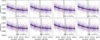 |
Fig. 7 Results of the box-shifting method. The shaded gray areas represent the searchboxes within which the mid-time of the lunar transit is constrained. The best-fit moon radius and its 1σ uncertainty is shown on the bottom of each plot. |
7 Discussion and concluding remarks
In this work, we have carried out a search for possible satellites orbiting the eccentric Neptune-sized planet HD 95338b in a sequential approach. Using four transits from CHEOPS and two from TESS, we present a detailed transit modelling, followed by a novel approach in the quest for exomoons. We re-derived the stellar parameters of the host star HD 95338, and present considerable improvements on some of them in comparison with the discovery paper (Díaz et al. 2020). We present improvements on the basic transit parameters of HD 95338b. Most notably, we reduce the uncertainty on the planetary radius by a factor of 10 compared to the results presented by Díaz et al. (2020). Given that the precision of these parameters does not change with the inclusion/exclusion of the two TESS transits, we argue that the stellar parameters and their uncertainties are properly taken into account in TLCM (as described in Csizmadia 2020) and that the uncertainties of the modelling parameters are limited by our knowledge of the star. The most remarkable improvement is achieved regarding the orbital period, which we estimate with a precision of ≈0.3 s compared to ≈1700 s in the discovery paper.
The quest for exomoons is difficult as we are trying to find transits whose timing and duration are not known, and that are shallow (especially in comparison with the instrumental noise effects of CHEOPS). A thorough detrending, incorporating all known noise sources is therefore a pre-requisite for such a project, as outlined in Sect. 2. We scanned the residual light curves after subtracting the planetary signal for signs of additional transit-like features that could be attributed to an exomoon orbiting HD 95338b. For a thorough characterisation of an exomoon which would incorporate the combination of two Keplerian orbits (Hippke & Heller 2022), at least three transit detections would be needed. We are able to rule out the presence of additional signals below ≈0.6 R⊕ at 1σ, thus placing an upper limit on the size of a hypothetical satellite in the system.
There are obvious long-term trends in the residuals seen in Fig. 2. With the assumption that these are linear (and letting the complex noise handling tools, either GP-based or wavelet-based, handle all other possible non-white noise realisations), we observed the detection of a transit-like feature (Fig. 6). However, with the addition of a quadratic trend (Figs. B.1 and 7), the transit detection is no longer significant. The deviation between the fitted linear and quadratic trends is the greatest around the position of the detected transit. The fact that the significance of the detection decreases after including a higher-order time-dependent term – which is commonly associated with astrophysical noise sources, such as spots – implies that the transit-like feature is likely not originated by a transit of an exomoon. Increasing the order of polynomials included in the modelling introduces the risk that the shorter timescale noise components are enhanced in a way that may introduce additional transit-like features. Thus we do not test for these possibilities, relying instead on the noise handling algorithms that are thought to be more efficient at higher frequencies. In any case, the retrieved moon size is consistent with a no-moon case at 3σ. Additionally, the lack of obvious TTVs (Fig. 5) also serves as counterargument against the presence of a satellite (Simon et al. 2007; Kipping 2009).
Based on the analysis of the synthetic LCs, we conclude that the method presented in Sect. 5 is viable for searching for exomoon transits in a non-photodynamical way. The injection-and -retrieval tests suggest that the combination of the sensitivity maps and the box-shifting method does not induce false positive detections, however, it does recover the size and position of the injected exomoon transits (within 2σ of their respective input values), and leads to >3σ detections even for the smallest tested moon sizes.
HD 95338b is an interesting target and an important milestone in the quest for exomoons. Future observations with CHEOPS, PLATO (PLAnetary Transits and Oscillations of stars Rauer et al. 2014, 2025), Ariel (Atmospheric Remote-sensing Infrared Exoplanet Large-survey Tinetti et al. 2018, 2022), or JWST (James Webb Space Telescope Gardner et al. 2006) may further reduce the current upper limit of 0.6 R⊕ on the radius of a possible moon in the system. The methodology presented in Sections 2 and 5 can also be regarded a stepping stone in the hunt for exomoons using the telescopes of the future. In the event of detections of additional signals that are similar to the one seen on Fig. 7, a fully photodynamic characterisation may be able to provide deeper insights into the nature of this system.
The discovery of the first confirmed exomoon will open a new chapter in exoplanet research. The above-told tale about the exomoon hunt around HD 95338b, together with the earlier examples mentioned in Section 1, sends a strong message to the research community regarding this subject. Detecting exomoons is currently situated at the frontiers of contemporary research, and success in confirming such discoveries can only be achieved through a comprehensive understanding and in-depth exploration of the intricacies involved in signal design, measurement techniques, and data analysis. Our discussion also outlines potential pathways to be explored during this investigation, and we are convinced that our considerations in the above analysis will provide significant methodological tools to this demanding task.
Data availability
The raw and detrended photometric time series data are available at the CDS via https://cdsarc.cds.unistra.fr/viz-bin/cat/J/A+A/701/A240
Acknowledgements
CHEOPS is an ESA mission in partnership with Switzerland with important contributions to the payload and the ground segment from Austria, Belgium, France, Germany, Hungary, Italy, Portugal, Spain, Sweden, and the United Kingdom. The CHEOPS Consortium would like to gratefully acknowledge the support received by all the agencies, offices, universities, and industries involved. Their flexibility and willingness to explore new approaches were essential to the success of this mission. CHEOPS data analysed in this article will be made available in the CHEOPS mission archive (https://cheops.unige.ch/archive_browser/). This work has made use of data from the European Space Agency (ESA) mission Gaia (https://www.cosmos.esa.int/gaia), processed by the Gaia Data Processing and Analysis Consortium (DPAC, https://www.cosmos.esa.int/web/gaia/dpac/consortium). Funding for the DPAC has been provided by national institutions, in particular the institutions participating in the Gaia Multilateral Agreement. On behalf of the ‘Searching for transiting exomoons in CHEOPS data’ project Sz.K. is grateful for the possibility to use HUN-REN Cloud (see Héder et al. 2022, https://science-cloud.hu/) which helped us achieve the results published in this paper. ASi and C.Br. acknowledge support from the Swiss Space Office through the ESA PRODEX program. A.De. Gy.M.Sz. acknowledges the support of the Hungarian National Research, Development and Innovation Office (NKFIH) grant K-125015, a a PRODEX Experiment Agreement No. 4000137122, the Lendúlet LP2018-7/2021 grant of the Hungarian Academy of Science and the support of the city of Szombathely. This project has received funding from the Swiss National Science Foundation for project 200021_200726. It has also been carried out within the framework of the National Centre of Competence in Research PlanetS supported by the Swiss National Science Foundation under grant 51NF40_205606. The authors acknowledge the financial support of the SNSF. T.Wi. acknowledges support from the UKSA and the University of Warwick. S.G.S. acknowledge support from FCT through FCT contract no. CEECIND/00826/2018 and POPH/FSE (EC). The Portuguese team thanks the Portuguese Space Agency for the provision of financial support in the framework of the PRODEX Programme of the European Space Agency (ESA) under contract number 4000142255. The Belgian participation to CHEOPS has been supported by the Belgian Federal Science Policy Office (BELSPO) in the framework of the PRODEX Program, and by the University of Liège through an ARC grant for Concerted Research Actions financed by the Wallonia-Brussels Federation. G.Sc., L.Bo., V.Na., I.Pa., G.Pi., R.Ra., and T.Zi. acknowledge support from CHEOPS ASI-INAF agreement no. 2019-29-HH.0. ABr was supported by the SNSA. YAl acknowledges support from the Swiss National Science Foundation (SNSF) under grant 200020_192038. We acknowledge financial support from the Agencia Estatal de Investigación of the Ministerio de Ciencia e Innovación MCIN/AEI/10.13039/501100011033 and the ERDF “A way of making Europe” through projects PID2019-107061GB-C61, PID2019-107061GB-C66, PID2021-125627OB-C31, and PID2021-125627OB-C32, from the Centre of Excellence “Severo Ochoa” award to the Instituto de Astrofísica de Canarias (CEX2019-000920-S), from the Centre of Excellence “María de Maeztu” award to the Institut de Ciències de l’Espai (CEX2020-001058-M), and from the Generalitat de Catalunya/CERCA programme. DBa, EPa, and IRi acknowledge financial support from the Agencia Estatal de Investigación of the Ministerio de Ciencia e Innovación MCIN/AEI/10.13039/501100011033 and the ERDF “A way of making Europe” through projects PID2019-107061GB-C61, PID2019-107061GB-C66, PID2021-125627OB-C31, and PID2021-125627OB-C32, from the Centre of Excellence “Severo Ochoa’ award to the Instituto de Astrofísica de Canarias (CEX2019-000920-S), from the Centre of Excellence “María de Maeztu” award to the Institut de Ciències de l’Espai (CEX2020-001058-M), and from the Generalitat de Catalunya/CERCA programme. SCCB acknowledges the support from Fundação para a Ciência e Tecnologia (FCT) in the form of work contract through the Scientific Employment Incentive program with reference 2023.06687.CEECIND. ACC acknowledges support from STFC consolidated grant number ST/V000861/1, and UKSA grant number ST/X002217/1. ACMC acknowledges support from the FCT, Portugal, through the CFisUC projects UIDB/04564/2020 and UIDP/04564/2020, with DOI identifiers https://doi.org/10.54499/UIDB/04564/2020 and https://doi.org/10.54499/UIDP/04564/2020, respectively. A.C., A.D., B.E., K.G., and J.K. acknowledge their role as ESA-appointed CHEOPS Science Team Members. P.E.C. is funded by the Austrian Science Fund (FWF) Erwin Schroedinger Fellowship, program J4595-N. This project was supported by the CNES. This work was supported by FCT – Fundação para a Ciência e a Tecnologia through national funds and by FEDER through COMPETE2020 through the research grants UIDB/04434/2020, UIDP/04434/2020, 2022.06962.PTDC. O.D.S.D. is supported in the form of work contract (DL 57/2016/CP1364/CT0004) funded by national funds through FCT. B.-O.D. acknowledges support from the Swiss State Secretariat for Education, Research and Innovation (SERI) under contract number MB22.00046. A.De., B.Ed., K.Ga., and J.Ko. acknowledge their role as ESA-appointed CHEOPS Science Team Members. C.B. acknowledges support from the Swiss NCCR PlanetS. This work has been carried out within the framework of the NCCR PlanetS supported by the Swiss National Science Foundation under grants 51NF40182901 and 51NF40205606. J.K. acknowledges support from the Swiss National Science Foundation under grant number TMSGI2_211697. MF and CMP gratefully acknowledge the support of the Swedish National Space Agency (DNR 65/19, 174/18). DG gratefully acknowledges financial support from the CRT foundation under Grant No. 2018.2323 “Gaseousor rocky? Unveiling the nature of small worlds”. M.G. is an F.R.S.-FNRS Senior Research Associate. CHe acknowledges the European Union H2020-MSCA-ITN-2019 under GrantAgreement no. 860470 (CHAMELEON), and the HPC facilities at the Vienna Science Cluster (VSC). MNG is the ESA CHEOPS Project Scientist and Mission Representative. BMM is the ESA CHEOPS Project Scientist. KGI was the ESA CHEOPS Project Scientist until the end of December 2022 and Mission Representative until the end of January 2023. All of them are/were responsible for the Guest Observers (GO) Programme. None of them relay/relayed proprietary information between the GO and Guaranteed Time Observation (GTO) Programmes, nor do/did they decide on the definition and target selection of the GTO Programme. K.W.F.L. was supported by Deutsche Forschungsgemeinschaft grants RA714/14-1 within the DFG Schwerpunkt SPP 1992, Exploring the Diversity of Extrasolar Planets. This work was granted access to the HPC resources of MesoPSL financed by the Region Ile de France and the project Equip@Meso (reference ANR-10-EQPX-29-01) of the programme Investissements d’Avenir supervised by the Agence Nationale pour la Recherche. This work has been carried out within the framework of the NCCR PlanetS supported by the Swiss National Science Foundation under grants 51NF40_182901 and 51NF40_205606. AL acknowledges support of the Swiss National Science Foundation under grant number TMSGI2_211697. ML acknowledges support of the Swiss National Science Foundation under grant number PCEFP2_194576. PM acknowledges support from STFC research grant number ST/R000638/1. This work was also partially supported by a grant from the Simons Foundation (PI Queloz, grant number 327127). NCSa acknowledges funding by the European Union (ERC, FIERCE, 101052347). Views and opinions expressed are however those of the author(s) only and do not necessarily reflect those of the European Union or the European Research Council. Neither the European Union nor the granting authority can be held responsible for them. V.V.G. is an F.R.S-FNRS Research Associate. JV acknowledges support from the Swiss National Science Foundation (SNSF) under grant PZ00P2_208945. EV acknowledges support from the ‘DISCOBOLO’ project funded by the Spanish Ministerio de Ciencia, Innovación y Universidades undergrant PID2021-127289NB-I00. NAW acknowledges UKSA grant ST/R004838/1. Project no. C1746651 has been implemented with the support provided by the Ministry of Culture and Innovation of Hungary from the National Research, Development and Innovation Fund, financed under the NVKDP-2021 funding scheme.
Appendix A Information about the CHEOPS observations
The metadata of the four CHEOPS observations are shown in Table A.1. The list of nearby stars, that may interfere with the aperture photometry, is shown in Table A.2.
File keys and the respective observation dates for the four CHEOPS visits of HD 95338.
List of stars that are (i) within 100” of HD 95338 and (ii) brighter than G = 15.2 magnitudes.
Appendix B Sensitivity maps
B.1 Quadratic trend
The sensitivity maps in case of a quadratic trend (for the real observations) are shown on Fig. B.1.
B.2 Synthetic transits
The results of injection-and-retrieval tests are shown in Figs. B.2 – B.5, and Tables B.1 – B.1.
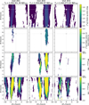 |
Fig. B.2 Same as Fig. 6 but with a quadratic trend instead of a linear trend and with an RMoon = 0.8 R⊕ moon injected into the first two visits. The injection-and retrieval tests were carried out only on the first three CHEOPS visits. |
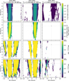 |
Fig. B.3 Same as Fig. B.2 but with a quadratic trend instead of a linear trend and with an RMoon = 1.35 R⊕ moon injected into the first two visits. |
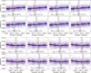 |
Fig. B.4 Performance of the box-shifting approach on the injected exomoon transits. Top rows: Recovery of an RMoon = 0.8 R⊕ in the first visit. Bottom row: Recovery of an RMoon = 0.8 R⊕ in the second visit. |
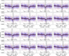 |
Fig. B.5 Performance of the box-shifting approach on the injected exomoon transits. Top row: Recovery of an RMoon = 1.35 R⊕ in the first visit. Bottom row: Recovery of an RMoon = 1.35 R⊕ in the second visit. |
Times of midtransit and recovered radii by the box-shifting method, of the injection-and-retrieval tests (T0,moon,injected = 2301.25) from the first visit.
Times of midtransit and recovered radii by the box-shifting method, of the injection-and-retrieval tests (T0,Moon,injected = 2687.05 from the first visit.
References
- Akaike, H. 1998, Information Theory and an Extension of the Maximum Likelihood Principle, eds. E. Parzen, K. Tanabe, & G. Kitagawa (New York, NY: Springer), 199 [Google Scholar]
- Barros, S. C. C., Demangeon, O., Díaz, R. F., et al. 2020, A&A, 634, A75 [EDP Sciences] [Google Scholar]
- Benz, W., Broeg, C., Fortier, A., et al. 2021, Exp. Astron., 51, 109 [Google Scholar]
- Blackwell, D. E., & Shallis, M. J. 1977, MNRAS, 180, 177 [NASA ADS] [CrossRef] [Google Scholar]
- Bonfanti, A., Ortolani, S., Piotto, G., & Nascimbeni, V. 2015, A&A, 575, A18 [NASA ADS] [CrossRef] [EDP Sciences] [Google Scholar]
- Bonfanti, A., Ortolani, S., & Nascimbeni, V. 2016, A&A, 585, A5 [NASA ADS] [CrossRef] [EDP Sciences] [Google Scholar]
- Bonfanti, A., Delrez, L., Hooton, M. J., et al. 2021, A&A, 646, A157 [EDP Sciences] [Google Scholar]
- Borucki, W. J., Koch, D., Basri, G., et al. 2010, Science, 327, 977 [Google Scholar]
- Carter, J. A., & Winn, J. N. 2009, ApJ, 704, 51 [Google Scholar]
- Castelli, F., & Kurucz, R. L. 2003, in Modelling of Stellar Atmospheres, eds. N. Piskunov, W. W. Weiss, & D. F. Gray, IAU Symposium, 210, A20 [Google Scholar]
- Csizmadia, S. 2020, MNRAS, 496, 4442 [Google Scholar]
- Csizmadia, S., Smith, A. M. S., Kálmán, S., et al. 2023, A&A, 675, A106 [NASA ADS] [CrossRef] [EDP Sciences] [Google Scholar]
- Díaz, M. R., Jenkins, J. S., Feng, F., et al. 2020, MNRAS, 496, 4330 [CrossRef] [Google Scholar]
- Dobos, V., Haris, A., Kamp, I. E. E., & van der Tak, F. F. S. 2022, MNRAS, 513, 5290 [NASA ADS] [CrossRef] [Google Scholar]
- Domingos, R. C., Winter, O. C., & Yokoyama, T. 2006, MNRAS, 373, 1227 [NASA ADS] [CrossRef] [Google Scholar]
- Ebden, M. 2015, arXiv e-prints [arXiv:1505.02965] [Google Scholar]
- Ehrenreich, D., Delrez, L., Akinsanmi, B., et al. 2023, A&A, 671, A154 [NASA ADS] [CrossRef] [EDP Sciences] [Google Scholar]
- Espinoza, N., & Jordán, A. 2015, MNRAS, 450, 1879 [Google Scholar]
- Foreman-Mackey, D., Hogg, D. W., Lang, D., & Goodman, J. 2013, PASP, 125, 306 [Google Scholar]
- Fortier, A., Simon, A. E., Broeg, C., et al. 2024, A&A, 687, A302 [NASA ADS] [CrossRef] [EDP Sciences] [Google Scholar]
- Fox, C., & Wiegert, P. 2021, MNRAS, 501, 2378 [NASA ADS] [CrossRef] [Google Scholar]
- Gaia Collaboration (Vallenari, A., et al.) 2023, A&A, 674, A1 [NASA ADS] [CrossRef] [EDP Sciences] [Google Scholar]
- Gardner, J. P., Mather, J. C., Clampin, M., et al. 2006, Space Sci. Rev., 123, 485 [Google Scholar]
- Gelman, A., & Rubin, D. B. 1992, Statist. Sci., 7, 457 [NASA ADS] [Google Scholar]
- Harre, J. V., Smith, A. M. S., Barros, S. C. C., et al. 2024, A&A, 692, A254 [NASA ADS] [CrossRef] [EDP Sciences] [Google Scholar]
- Héder, M., Rigó, E., Medgyesi, D., et al. 2022, Inform. Társadalom, 22, 128 [Google Scholar]
- Heller, R., & Hippke, M. 2024, Nat. Astron., 8, 193 [Google Scholar]
- Heller, R., Rodenbeck, K., & Bruno, G. 2019, A&A, 624, A95 [NASA ADS] [CrossRef] [EDP Sciences] [Google Scholar]
- Hippke, M., & Heller, R. 2022, A&A, 662, A37 [NASA ADS] [CrossRef] [EDP Sciences] [Google Scholar]
- Hoyer, S., Guterman, P., Demangeon, O., et al. 2020, A&A, 635, A24 [NASA ADS] [CrossRef] [EDP Sciences] [Google Scholar]
- Husser, T. O., Wende-von Berg, S., Dreizler, S., et al. 2013, A&A, 553, A6 [NASA ADS] [CrossRef] [EDP Sciences] [Google Scholar]
- Kálmán, S., Csizmadia, S., Simon, A. E., et al. 2024a, MNRAS, 528, L66 [Google Scholar]
- Kálmán, S., Derekas, A., Csizmadia, S., et al. 2024b, A&A, 687, A144 [NASA ADS] [CrossRef] [EDP Sciences] [Google Scholar]
- Kálmán, S., Szabó, G. M., Borsato, L., et al. 2023a, MNRAS, 522, 488 [CrossRef] [Google Scholar]
- Kálmán, S., Szabó, G. M., & Csizmadia, S. 2023b, A&A, 675, A107 [NASA ADS] [CrossRef] [EDP Sciences] [Google Scholar]
- Kiefer, F., Van Grootel, V., Lecavelier des Etangs, A., et al. 2023, A&A, 671, A25 [NASA ADS] [CrossRef] [EDP Sciences] [Google Scholar]
- Kipping, D. M. 2009, MNRAS, 392, 181 [NASA ADS] [CrossRef] [Google Scholar]
- Kipping, D. 2020, ApJ, 900, L44 [NASA ADS] [CrossRef] [Google Scholar]
- Kipping, D. 2021, MNRAS, 507, 4120 [NASA ADS] [CrossRef] [Google Scholar]
- Kipping, D., & Yahalomi, D. A. 2023, MNRAS, 518, 3482 [Google Scholar]
- Kipping, D. M., Schmitt, A. R., Huang, X., et al. 2015, ApJ, 813, 14 [NASA ADS] [CrossRef] [Google Scholar]
- Kipping, D., Bryson, S., Burke, C., et al. 2022, Nat. Astron., 6, 367 [NASA ADS] [CrossRef] [Google Scholar]
- Kipping, D., Teachey, A., Yahalomi, D. A., et al. 2025, Nat. Astron., 9, 795 [Google Scholar]
- Kreidberg, L., Luger, R., & Bedell, M. 2019, ApJ, 877, L15 [NASA ADS] [CrossRef] [Google Scholar]
- Krenn, A. F., Kubyshkina, D., Fossati, L., et al. 2024, A&A, 686, A301 [NASA ADS] [CrossRef] [EDP Sciences] [Google Scholar]
- Kurucz, R. L. 1979, ApJS, 40, 1 [NASA ADS] [CrossRef] [Google Scholar]
- Kurucz, R. L. 1993, SYNTHE spectrum synthesis programs and line data [Google Scholar]
- Lacedelli, G., Wilson, T. G., Malavolta, L., et al. 2022, MNRAS, 511, 4551 [NASA ADS] [CrossRef] [Google Scholar]
- Lindegren, L., Bastian, U., Biermann, M., et al. 2021, A&A, 649, A4 [EDP Sciences] [Google Scholar]
- Luger, R., Lustig-Yaeger, J., & Agol, E. 2017, ApJ, 851, 94 [NASA ADS] [CrossRef] [Google Scholar]
- Marigo, P., Girardi, L., Bressan, A., et al. 2017, ApJ, 835, 77 [Google Scholar]
- Mayor, M., & Queloz, D. 1995, Nature, 378, 355 [Google Scholar]
- Rasmussen, C. E., & Williams, C. K. I. 2006, Gaussian Processes for Machine Learning [Google Scholar]
- Rauer, H., Catala, C., Aerts, C., et al. 2014, Exp. Astron., 38, 249 [Google Scholar]
- Rauer, H., Aerts, C., Cabrera, J., et al. 2025, Exp. Astron., 59, 26 [Google Scholar]
- Ricker, G. R., Winn, J. N., Vanderspek, R., et al. 2015, J. Astron. Telesc. Instrum. Syst., 1, 014003 [Google Scholar]
- Ripley, B. D. 1987, Stochastic simulation (New York, NY, USA: John Wiley & Sons, Inc.) [Google Scholar]
- Roberts, S., Osborne, M., Ebden, M., et al. 2012, Philos. Trans. Roy. Soc. Lond. Ser. A, 371, 20110550 [Google Scholar]
- Saha, S. 2025, MNRAS, 539, 928 [Google Scholar]
- Saha, S., & Sengupta, S. 2022, ApJ, 936, 2 [NASA ADS] [CrossRef] [Google Scholar]
- Salmon, S. J. A. J., Van Grootel, V., Buldgen, G., Dupret, M. A., & Eggenberger, P. 2021, A&A, 646, A7 [NASA ADS] [CrossRef] [EDP Sciences] [Google Scholar]
- Santos, N. C., Sousa, S. G., Mortier, A., et al. 2013, A&A, 556, A150 [NASA ADS] [CrossRef] [EDP Sciences] [Google Scholar]
- Scandariato, G., Carone, L., Cubillos, P. E., et al. 2024, A&A, 692, A129 [NASA ADS] [CrossRef] [EDP Sciences] [Google Scholar]
- Schanche, N., Hébrard, G., Collier Cameron, A., et al. 2020, MNRAS, 499, 428 [NASA ADS] [CrossRef] [Google Scholar]
- Schwarz, G. 1978, Ann. Statist., 6, 461 [Google Scholar]
- Scuflaire, R., Théado, S., Montalbán, J., et al. 2008, Ap&SS, 316, 83 [Google Scholar]
- Simon, A., Szatmáry, K., & Szabó, G. M. 2007, A&A, 470, 727 [NASA ADS] [CrossRef] [EDP Sciences] [Google Scholar]
- Simon, A. E., Szabó, G. M., Kiss, L. L., Fortier, A., & Benz, W. 2015, PASP, 127, 1084 [CrossRef] [Google Scholar]
- Skrutskie, M. F., Cutri, R. M., Stiening, R., et al. 2006, AJ, 131, 1163 [NASA ADS] [CrossRef] [Google Scholar]
- Smith, A. M. S., & Csizmadia, S. 2022, AJ, 164, 21 [NASA ADS] [CrossRef] [Google Scholar]
- Sneden, C. A. 1973, PhD thesis, The University of Texas at Austin [Google Scholar]
- Sousa, S. G. 2014, arXiv e-prints [arXiv:1407.5817] [Google Scholar]
- Sousa, S. G., Santos, N. C., Israelian, G., Mayor, M., & Monteiro, M. J. P. F. G. 2007, A&A, 469, 783 [NASA ADS] [CrossRef] [EDP Sciences] [Google Scholar]
- Sousa, S. G., Santos, N. C., Adibekyan, V., Delgado-Mena, E., & Israelian, G. 2015, A&A, 577, A67 [NASA ADS] [CrossRef] [EDP Sciences] [Google Scholar]
- Sousa, S. G., Adibekyan, V., Delgado-Mena, E., et al. 2021, A&A, 656, A53 [NASA ADS] [CrossRef] [EDP Sciences] [Google Scholar]
- Southworth, J. 2011, MNRAS, 417, 2166 [Google Scholar]
- Szabó, G. M., Szatmáry, K., Divéki, Z., & Simon, A. 2006, A&A, 450, 395 [NASA ADS] [CrossRef] [EDP Sciences] [Google Scholar]
- Szabó, G. M., Gandolfi, D., Brandeker, A., et al. 2021, A&A, 654, A159 [NASA ADS] [CrossRef] [EDP Sciences] [Google Scholar]
- Szabó, G. M., Schneider, J., Dencs, Z., & Kálmán, S. 2024, Universe, 10, 110 [Google Scholar]
- Teachey, A., & Kipping, D. M. 2018, Sci. Adv., 4, eaav1784 [Google Scholar]
- Ter Braak, C. J. F. 2006, Statist. Comput., 16, 239 [Google Scholar]
- Tinetti, G., Drossart, P., Eccleston, P., et al. 2018, Exp. Astron., 46, 135 [NASA ADS] [CrossRef] [Google Scholar]
- Tinetti, G., Eccleston, P., Lueftinger, T., et al. 2022, in European Planetary Science Congress, EPSC2022-1114 [Google Scholar]
- Tsantaki, M., Sousa, S. G., Adibekyan, V. Z., et al. 2013, A&A, 555, A150 [NASA ADS] [CrossRef] [EDP Sciences] [Google Scholar]
- Wade, R. A., & Rucinski, S. M. 1985, A&AS, 60, 471 [NASA ADS] [Google Scholar]
- Wright, E. L., Eisenhardt, P. R. M., Mainzer, A. K., et al. 2010, AJ, 140, 1868 [Google Scholar]
On 11/06/2024, the NASA Exoplanet Archive listed 5787 confirmed planets, https://exoplanetarchive.ipac.caltech.edu/
In our experiments, with the available CPUs, the fitting the FBV parameters jointly can be accomplished in ~1 month, instead of the several hour long runtimes needed with the pre-whitening approach that we implemented.
The last version, ARES v2, can be downloaded at https://github.com/sousasag/ARES
PAdova and TRieste Stellar Evolutionary Code: http://stev.oapd.inaf.it/cgi-bin/cmd
We assumed that [Fe/H] = [M/H].
The Hill sphere defines the gravitational sphere of influence of a body and is therefore where moons are expected to exist. Domingos et al. (2006) shows that beyond half the Hill sphere radius, only retrograde orbits are stable, and we cover the full radius not to exclude these potential objects.
All Tables
Transit timing data (and other selected parameters from the transit modelling) of HD 95338b.
Temporal coordinates of the eight searchboxes used in the box-shifting analysis of the exomoon signal seen in the third visit, and the best-fit parameters describing the correlated noise, the transit, and the long-term trend.
File keys and the respective observation dates for the four CHEOPS visits of HD 95338.
List of stars that are (i) within 100” of HD 95338 and (ii) brighter than G = 15.2 magnitudes.
Times of midtransit and recovered radii by the box-shifting method, of the injection-and-retrieval tests (T0,moon,injected = 2301.25) from the first visit.
Times of midtransit and recovered radii by the box-shifting method, of the injection-and-retrieval tests (T0,Moon,injected = 2687.05 from the first visit.
All Figures
|
Fig. 1 The Subarray image depicts the point spread function (PSF) of HD 95338b and the neighbouring stars, with their respective magnitudes of brightness indicated. The target is centred on the coordinates (180, 178) on the CCD. |
| In the text | |
|
Fig. 2 Demonstration of the fitting and detrending steps. The raw CHEOPS light curves of HD 95338b are shown in the top row, along with the initially fitted transit curves (step 1). The residuals of the initial transit fit, along with the best-fit systematics model is shown in the second row, with N number of harmonics of the roll angle included. The final transit fit (step 4) and its residuals (later used in the search for additional transits) are shown in the bottom two rows, where the full white circles represent 200-point bins (with an average uncertainty of ≈20 ppm in each bin). |
| In the text | |
|
Fig. 3 Phase-folded detrended CHEOPS light curve of HD 95338 (top panel, orange; same data as the third row of Fig. 2.) The rednoise-corrected light curve is shown with blue, while the best-fit transit light curves of HD 95338b is represented by the solid red curve. |
| In the text | |
|
Fig. 4 Phase-folded detrended TESS light curve of HD 95338 (top panel, orange, the same data as the third row of Fig. 2.) The rednoise-corrected light curve is shown with blue, while the best-fit transit light curves of HD 95338b is represented by the solid red curve. |
| In the text | |
|
Fig. 5 Transit timing data of HD 95338b. The dashed purple lines represent the uncertainty range from the global fit. |
| In the text | |
|
Fig. 6 Sensitivity maps for the four CHEOPS visits of HD 95338. The first row represents the best-fit box depth (i.e. moon radius) in the ΔT0−W space. The 3σ lower limit of the moon radius is shown in the second row, while the third and fourth rows represent the ΔBIC and ΔAIC values between a solution with and without a moon. The empty (blank) areas are values that are below a threshold of 0 R⊕ for the moon radius (first 2 rows) and a threshold of 2 for the ΔBIC and ΔAIC (last 2 rows). The grey squares (and corresponding dotted lines) show the position of the transit of HD 95338b in this parameter space for each visit. An underlying linear trend is assumed for each of the four visits. |
| In the text | |
|
Fig. 7 Results of the box-shifting method. The shaded gray areas represent the searchboxes within which the mid-time of the lunar transit is constrained. The best-fit moon radius and its 1σ uncertainty is shown on the bottom of each plot. |
| In the text | |
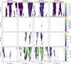 |
Fig. B.1 Same as Fig. 6 but with a quadratic trend instead of a linear trend. |
| In the text | |
|
Fig. B.2 Same as Fig. 6 but with a quadratic trend instead of a linear trend and with an RMoon = 0.8 R⊕ moon injected into the first two visits. The injection-and retrieval tests were carried out only on the first three CHEOPS visits. |
| In the text | |
|
Fig. B.3 Same as Fig. B.2 but with a quadratic trend instead of a linear trend and with an RMoon = 1.35 R⊕ moon injected into the first two visits. |
| In the text | |
|
Fig. B.4 Performance of the box-shifting approach on the injected exomoon transits. Top rows: Recovery of an RMoon = 0.8 R⊕ in the first visit. Bottom row: Recovery of an RMoon = 0.8 R⊕ in the second visit. |
| In the text | |
|
Fig. B.5 Performance of the box-shifting approach on the injected exomoon transits. Top row: Recovery of an RMoon = 1.35 R⊕ in the first visit. Bottom row: Recovery of an RMoon = 1.35 R⊕ in the second visit. |
| In the text | |
Current usage metrics show cumulative count of Article Views (full-text article views including HTML views, PDF and ePub downloads, according to the available data) and Abstracts Views on Vision4Press platform.
Data correspond to usage on the plateform after 2015. The current usage metrics is available 48-96 hours after online publication and is updated daily on week days.
Initial download of the metrics may take a while.