| Issue |
A&A
Volume 701, September 2025
|
|
|---|---|---|
| Article Number | A54 | |
| Number of page(s) | 11 | |
| Section | Astrophysical processes | |
| DOI | https://doi.org/10.1051/0004-6361/202554099 | |
| Published online | 02 September 2025 | |
An unusual type-I X-ray burst from the neutron star X-ray binary IGR J17591–2342: A possible double-photospheric radius-expansion burst
1
Department of Astronomy and Astrophysics, Tata Institute of Fundamental Research, 1 Homi Bhabha Road, Colaba Mumbai 400005, India
2
Department of Physics, Bar-Ilan University, Ramat-Gan 52900, Israel
3
Dipartimento di Fisica, Università degli Studi di Cagliari, SP Monserrato-Sestu, KM 0.7, Monserrato I-09042, Italy
4
INFN, Sezione di Cagliari, Cittadella Universitaria, I-09042 Monserrato, CA, Italy
⋆ Corresponding authors: This email address is being protected from spambots. You need JavaScript enabled to view it.
, This email address is being protected from spambots. You need JavaScript enabled to view it.
, This email address is being protected from spambots. You need JavaScript enabled to view it.
Received:
10
February
2025
Accepted:
16
June
2025
Abstract
Context. The type-I X-ray bursts observed from neutron stars originate from the intermittent unstable thermonuclear burning of accreted matter on these stars. Such bursts, particularly those reaching the Eddington luminosity and having a temporary photospheric radius expansion due to radiation pressure, provide a testbed to study nuclear fusion processes in intense radiation, gravity, and magnetic fields.
Aims. Here, we investigate time-resolved spectroscopic properties of a type-I burst from the accretion-powered millisecond X-ray pulsar IGR J17591–2342.
Methods. Our basic spectral model includes an absorbed blackbody to describe the burst emission and an absorbed power law to represent the non-burst emission.
Results. The blackbody normalisation shows two consecutive humps aligned with blackbody temperature dips during the burst. Such an unusual behaviour could imply two consecutive photospheric radius-expansion events during the same burst or a systematic metallicity evolution in the neutron star atmosphere. However, our spectral analysis suggests the latter option is less likely to be happening for IGR J17591–2342.
Conclusions. The novel former option implies that sufficient fuel survived after the first photospheric radius-expansion event to power a second similar event a few seconds later and thus challenges current theoretical understanding. If confirmed, the double-photospheric radius-expansion event observed in IGR J17591–2342 suggests the possibility of avoiding photospheric expansion at luminosities exceeding Eddington. Mechanisms such as temporary enhancement of the magnetic field by convection and confinement of the plasma could be invoked to explain the peculiar behaviour of the source.
Key words: accretion / accretion disks / methods: data analysis / stars: neutron / pulsars: individual: IGR J17591-2342 / X-rays: binaries / X-rays: bursts
© The Authors 2025
 Open Access article, published by EDP Sciences, under the terms of the Creative Commons Attribution License (https://creativecommons.org/licenses/by/4.0), which permits unrestricted use, distribution, and reproduction in any medium, provided the original work is properly cited.
This article is published in open access under the Subscribe to Open model. This email address is being protected from spambots. You need JavaScript enabled to view it. to support open access publication.
1. Introduction
A neutron star low-mass X-ray binary (LMXB) primarily emits X-rays due to the mass transfer from a low-mass companion star to a neutron star via an accretion disc (Bhattacharya & van den Heuvel 1991). This accreted matter, or fuel, accumulates on the stellar surface and can intermittently burn via thermonuclear runaway fusion processes, giving rise to a burst of radiation observed in X-rays, typically for several tens of seconds (Grindlay et al. 1976; Lamb & Lamb 1978; Strohmayer & Bildsten 2006; Galloway et al. 2020, and references therein). Such a burst, known as a type-I X-ray burst, is expected to ignite at a certain point on the star. Then the thermonuclear flames may spread to engulf the entire surface, typically, during the early part of the burst rise (Spitkovsky et al. 2002; Bhattacharyya & Strohmayer 2007; Chakraborty & Bhattacharyya 2014). Variations in X-ray intensity with frequencies close to the neutron star’s spin frequency have been detected for some bursts. These burst oscillations may originate from an azimuthally asymmetric brightness pattern on the spinning stellar surface (Watts 2012; Bhattacharyya 2022). Notably, the spectral and timing aspects of thermonuclear bursts can be useful for probing the superdense matter in the neutron star core (Bhattacharyya 2010, and references therein) and the plasma and nuclear physics in the strong gravity regime (Strohmayer & Bildsten 2006).
It is particularly important to study some of these topics for the most intense bursts, such as photospheric radius-expansion (PRE) bursts, for which the burst luminosity temporarily exceeds the Eddington luminosity (Shapiro & Teukolsky 1983; Galloway et al. 2020; Strohmayer et al. 2019). For this luminosity, the outward radiative force temporarily exceeds the inward gravitational force, pushing the stellar photosphere away from the star. We note that the identification and study of these phenomena require tracking of the evolution of burst spectral and timing properties using a time-resolved analysis (e.g. Bhattacharyya & Strohmayer 2006; Bult et al. 2019). Findings from such an analysis have shown that the temperature of the photosphere decreases as it expands and increases again as the photosphere contracts and touches the neutron star surface.
This paper reports the results of a study that applied time-resolved spectroscopy to a peculiar type-I X-ray burst observed from the neutron star LMXB IGR J17591–2342. This source is an accretion-powered millisecond X-ray pulsar (AMXP) with a spin frequency of ≈527.4 Hz, for which the neutron star magnetosphere channels the accreted matter to stellar magnetic poles (Sanna et al. 2018; Bhattacharya & van den Heuvel 1991). Kuiper et al. (2020) reported a type-I burst from this source. They concluded that this was most likely a PRE burst from its fast rise (∼1 − 2 s) and a subsequent ∼10 s long plateau at its peak, but they did not use time-resolved spectroscopy. Here, a study using time-resolved spectroscopy of another type-I burst observed earlier with AstroSat suggests an unusual nature: two likely consecutive PRE events within a few seconds during the same burst. An interpretation of this novel scenario concerns two of the most crucial questions regarding such type-I X-ray bursts, namely, whether the available magnetic field can confine the plasma during a nuclear fusion, and whether a significant amount of fuel in the vicinity of the burning region can remain unburnt. We present the observation of IGR J17591–2342 in Section 2, describe colour and pre-burst spectral analysis in Section 3, detail burst spectral analysis in Section 4, and discuss the results and interpretation in Section 5.
2. Observation
The AMXP IGR J17591–2342 was observed with AstroSat Large Area X-ray Proportional Counters1 (LAXPCs; Antia et al. 2017, 2021) in event mode from 2018-08-23T01:03:50 to 2018-08-24T00:35:00 UTC (Observation ID (ObsID): 9000002320). The data are, however, not continuous because AstroSat is a low Earth orbit satellite, and there are Earth occultation and South Atlantic Anomaly passages (Seetha & Kasturirangan 2021). The energy range, area, and time resolution of LAXPC are ≈3 − 80 keV, ∼6000 cm2, and ≈10 μs, respectively (Antia et al. 2017). We used one LAXPC detector, LAXPC20, because the other two detectors had leak and gain stability issues (Antia et al. 2021). Using the laxpc3.4.3 software, we analysed the LAXPC data; extracted light curves, spectra, background, and response files; and corrected the effects of deadtime in light curves and spectra. We note that blank sky observations were used to estimate the LAXPC background. We identified a type-I X-ray burst due to its typical sharp rise, top plateau-type portion, and near-exponential decay (see Figure 1). This burst, which occurred on August 23, 2018, started around 03:38:31 UTC. In this paper, we probe and interpret the spectral evolution of this burst.
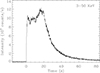 |
Fig. 1. X-ray (3 − 50 keV) intensity versus time (with 0.1 s bins) of a thermonuclear type-I burst observed from the accreting millisecond X-ray pulsar IGR J17591–2342 with AstroSat/LAXPC (Section 2). |
We note that a recent paper, (Manca et al. 2023), mentioned an unexpected spectral nature of the source during the ObsID 9000002320, which they speculate could have been due to ‘a bad calibration’. However, we find that the spectral nature was due to a large intensity increase, which was observed with LAXPC during a part of this ObsID (see also Singh et al. 2025). This increase was not due to the X-ray intensity increase of IGR J17591–2342, as we confirmed from a few short observations with the NICER satellite (Manca et al. 2023) conducted during the AstroSat ObsID 9000002320. We note that there was no NICER observation during the type-I X-ray burst. The LAXPC count rate increase was due to a drift of the satellite pointing from IGR J17591–2342 towards a nearby bright persistent source GX 5–1 (confirmed from a discussion with the LAXPC team; see also Singh et al. 2025). However, the type-I X-ray burst occurred during the initial part of the ObsID 9000002320, when the LAXPC count rate increase had not yet begun, and the observed spectrum is consistent with the expected source spectrum. Therefore, our burst and pre-burst spectra are genuinely from IGR J17591–2342 and are free of any calibration problem.
3. Colour estimation and pre-burst spectral analysis
To study the evolution of the burst properties, we divided the first 45 seconds of the burst into one-second time bins. First, we studied the colour evolution during the burst, which gives a model-independent overview of the source spectral evolution and provides a sanity check for the spectral results. We defined the colour, or softness, as the background-subtracted count rate ratio between 3 − 6 keV (channels 5 − 10) and 12 − 15 keV (channels 22 − 27). Panels a–c of Figure 2 show the profiles of the 3 − 6 keV count rate, 12 − 15 keV count rate, and softness. The softness has two clear consecutive humps followed by an increase, which suggest a preliminary softening of the source spectrum followed by two hardening phases, after which the source continued to soften during the rest of the burst.
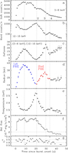 |
Fig. 2. Time-resolved (1s bins) properties with 1σ errors of the thermonuclear X-ray burst observed from IGR J17591–2342 with AstroSat/LAXPC. Panels a–c: Background-subtracted count rates in the energy range 3 − 6 keV, 12 − 15 keV, and their ratio, respectively. Panels d–f: Blackbody radius (rBB/D10), blackbody temperature kTBB, and bolometric (0.01–100 keV) blackbody flux FBB from the burst intervals best fits using the model tbabs(bbodyrad+constant*powerlaw+gauss+gauss) (see Sections 3, 4 and 5 for more details). The dotted horizontal line marks the FBB at the second touchdown point (see Section 5.2). Panel g: Reduced χ2 of spectral fits. |
In line with the standard relatively short pre-burst interval selection (Jaisawal et al. 2019), we generated a pre-burst spectrum for the 200 s interval just before the burst onset to ensure at least 25 counts in each bin. We modelled the LAXPC non-burst spectrum of IGR J17591–2342 with an absorbed Comptonization model (tbabs*Nthcomp in XSPEC), in line with the detailed analysis performed on a broader energy range combining multiple available datasets (see Manca et al. 2023, for more details). Due to the lack of coverage below 3 keV, we do not include an edge kept fixed at 0.871 keV by Manca et al. (2023) and froze the hydrogen column density at 2.25 × 1022 cm−2 (Kuiper et al. 2020). Finally, we included a 3% systematic uncertainty for the LAXPC spectral fitting (Maqbool et al. 2019).
The reduced χ2 (χν2 = χ2/d.o.f.; d.o.f. is degrees of freedom) is ≈1.55 (51/33), and the absorbed flux is ∼3 × 10⁻¹⁰ erg s−1 cm−2 for the XSPEC model tbabs*Nthcomp fit in the 3 − 25 keV range. The addition of a blackbody component does not improve the fit. This aligns with Manca et al. (2023), which only sporadically detected a significant blackbody contribution during the outburst, characterised by a temperature of 0.8 ± 0.2 keV, outside the LAXPC energy range. We note that the addition of a Gaussian around 6.6 keV marginally improves the χν2(d.o.f.) to ≈1.38(30). However, since a Gaussian component in the ∼6 − 8 keV range would later be included to describe the burst spectrum, we decided not to include it for the pre-burst modelling.
We also explored if an absorbed power-law model (tbabs*powerlaw in XSPEC) could adequately describe the pre-burst spectrum. We obtained a χν2(d.o.f.) of ≈1.44(35) for the best-fit power-law photon index and a normalisation of 2.10 ± 0.04 and 0.11 ± 0.01, respectively. Since the power-law component mimics the Comptonization well, we used it to describe the pre-burst emission for most spectral fits. In addition to ensuring a similar χ2 value for a lesser number of free parameters (compared to that for tbabs*Nthcomp), the tbabs*powerlaw model allowed us to explore the effects of an evolving non-burst spectral shape only by keeping a single parameter free (the power-law photon index), while for Nthcomp several free parameters are required. Nevertheless, for completeness, we also tested the burst spectral fits using Nthcomp to describe the non-burst spectrum.
4. Burst spectra: Analysis, results, and interpretation
After characterising a pre-burst spectrum of IGR J17591–2342, we modelled the spectra of the first 45 independent burst time bins, each of 1 s. We also modelled the spectra of the first 22 independent burst time bins, each of 2 s, to show that the conclusions do not depend on the choice of the bin size. Similar to the pre-burst spectral analysis (see Section 3), we ensured that there are at least 25 counts in each spectral bin, used 3% systematics, froze the hydrogen column density at 2.25 × 1022 cm−2, and fit in the 3 − 25 keV range (3 − 12 keV only for the third 1 s time bin, which shows systematics at higher energies).
4.1. Basic model
The burst spectra are usually fit with a blackbody (bbodyrad in XSPEC) model (Galloway et al. 2008), which has two parameters: temperature (kTBB; k is the Boltzmann constant) and normalisation (NBB = rBB2/D102). Throughout this paper, we use rBB/D10 to refer to the blackbody radius, where D10 is the source distance in units of 10 kpc. The blackbody effective temperature of the neutron star photosphere (kTeff) shifts to a higher value (colour temperature kTc) due to electron scattering in the stellar atmosphere (London et al. 1986), and hence, the blackbody here is diluted. We inferred the effective temperature, kTeff, by rescaling the observed temperature, kTBB, by the factor (1 + zr)/fc, where fc is the colour factor and 1 + zr = [1 − (2GM/rc2)]−1/2 for Schwarzschild spacetime. Here, G and M are the gravitational constant and neutron star mass, respectively (Shapiro & Teukolsky 1983; Damen et al. 1990). Similarly, the photospheric radius, r, was inferred by rescaling rBB by the factor fc2/(1 + zr).
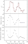 |
Fig. 3. Time-resolved (2 s bins) properties, with 1σ errors, of the thermonuclear X-ray burst observed from IGR J17591–2342 with AstroSat/LAXPC (see Section 4.1). The upper panel shows reduced χ2 profiles for the spectral fitting with the XSPEC models tbabs(bbodyrad+constant*powerlaw) (black; power-law parameter values frozen to the pre-burst values) and tbabs(bbodyrad+powerlaw) (red). This panel shows that the fitting is not acceptable. Overall, the fitting does not improve when the spectral shape (power-law photon index) is made free, and the reduced χ2 profiles have two humps. The middle and lower panels show the blackbody (bbodyrad) parameter (radius and temperature, respectively) profiles for the first model mentioned above. These panels (along with the dotted vertical lines) show that radius humps and temperature dips coincide with the reduced χ2 humps. |
In order to account for both the pre-burst and burst components, we used the XSPEC model tbabs(bbodyrad+constant*powerlaw), which should be considered the basic model for burst spectra. The power-law component has frozen pre-burst best-fit value parameters, while the free energy-independent constant allows for possible flux variations of the pre-burst emission during the burst. We note that while this is the standard way to describe the non-burst emission during the burst (see e.g. Jaisawal et al. 2019), we also performed fits with a free power-law photon index parameter to investigate a possible evolution of the pre-burst spectral shape. Furthermore, while an absorbed power law adequately describes the pre-burst spectrum (as shown in section 3), we also replaced it with a Comptonization model component to check the reliability of our results.
For the fitting with the tbabs(bbodyrad+constant*powerlaw) model, we obtained high and unacceptable χν2 values for most of the intervals (upper panel, Figure 3). This suggests that the basic model does not adequately describe the data. We note that two humps of the burst blackbody radius (rBB/D10) profile are clearly seen in Figure 3, which are aligned with the blackbody temperature (kTBB) dips. Interestingly, the two χν2 humps align with the two humps of radius and the two dips of temperature of the blackbody component. For example, for the above-mentioned basic model, χν2(d.o.f.) at the burst onset (1.62(34)) monotonically increases to 4.88(29) after about 9 s. It then decreases and reaches a minimum of 1.51(34) after about 21 s from the burst onset. It monotonically increases again to 4.46(22) after about 29 s from the burst onset and then decreases again. This shows that the basic spectral model is particularly inadequate during the two humps of radius and two dips of temperature of the blackbody component. We tested whether the inadequacy of the basic model derives from an evolution of the power-law photon index; however, leaving the photon index free did not significantly improve the fits (Figure 3).
4.2. Model with reflection and double-PRE interpretation
We examined the data-to-model ratio from the spectral fitting to understand why the χν2 values are high for the basic model. We generally found two excesses contributing the most in the ∼6 − 8 keV and ∼12 − 20 keV ranges of the data-to-model ratio profile (see e.g. Figure 4). Fitting the two excesses with Gaussian components decreases the χν2(d.o.f) from 4.88(29) to 1.95(26) (Gaussian for ∼6 − 8 keV) and finally to 1.22(23) (Gaussian also for ∼12 − 20 keV). Based on that, we updated the model to tbabs(bbodyrad+constant*powerlaw+gauss+gauss) for all burst time bins to perform a uniform spectral analysis. However, we also verified our results with only the ∼6 − 8 keV Gaussian for those time bins for which the ∼12 − 20 keV excess is not prominent.
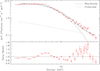 |
Fig. 4. Spectral fitting for the thermonuclear X-ray burst observed from IGR J17591–2342 with AstroSat/LAXPC (see Section 4.2). The spectrum is for 8 − 10 s since the burst onset, and the XSPEC model is tbabs(bbodyrad+constant*powerlaw) with the powerlaw parameter values frozen to the pre-burst values (Section 3). Upper panel: Unfolded spectrum. Data with 1σ errors are shown in red. The total model (solid histogram), tbabs*bbodyrad component (dashed line), and tbabs*constant*powerlaw component (dotted line) are also shown. Lower panel: Data-to-model ratio with errors. This figure shows that this model is not adequate because there are two excesses in the ∼6 − 8 keV and ∼12 − 20 keV ranges. |
As shown in panel g of Figure 2, the updated model provides χν2 values always lower than two (for 1 s burst time bins), ∼80% of which are lower than 1.5. Considering a χν2 standard deviation of ∼0.3 for a mean d.o.f. of ∼17, the limited statistics for the selected short intervals, and the modest spectral resolution of LAXPC, we regard the fits as acceptable, so we included no further components.
Before presenting the evolution of the blackbody parameter values, we discuss our interpretation of the other model components. As previously mentioned in Section 3, the power-law component represents the Comptonization component from the non-burst emission. The flux of this component increases during the burst, as can be seen from a significant increase of the constant component (on average ∼27 for burst time bins), likely reflecting an enhancement of the accretion rate caused by the radiation-induced Poynting–Robertson drag on the accretion disc (Walker 1992; Worpel et al. 2013). However, the direct disc emission is not spectrally detected due to the limited LAXPC energy range at relatively low energies.
The two Gaussian components can be naturally described as features of the reflection spectrum off the accretion disc, with the ∼6 − 8 keV component representing the Fe Kα line, while the ∼12 − 20 keV component is associated with the Compton back-scattering (Ballantyne 2004; Miller 2007). Such a reflection spectrum during thermonuclear bursts has been observationally reported earlier (Guver et al. 2022). We note that photons from both the burst and Comptonization components should have been reflected off the disc, and hence, a complex reflection model is required to describe the spectrum. We tested whether the model for burst photon reflection off the accretion disc (bbrefl in XSPEC; Ballantyne 2004) and the model pexmon (XSPEC) for reflection of photons from a Comptonization (cut-off power law) component give acceptable fits for most of the burst time bins, indicating contributions from both may be required.
Next, we consider the evolution of blackbody parameter values. Panels d–e of Figure 2 show the profiles of the best-fit blackbody (bbodyrad) parameters: radius (rBB/D10) and temperature (kTBB). The blackbody radius profile shows two consecutive humps that are aligned with temperature dips. This peculiar behaviour is consistent with two subsequent PRE events, each of which is compatible with the typical increase (decrease) and subsequent decrease (increase) of the blackbody radius (blackbody temperature) (see e.g. Galloway et al. 2020). However, while a PRE event during a strong thermonuclear burst is common, a second PRE during the same type-I X-ray burst is not typically expected or detected. Therefore, we first needed to establish the reliability of the second blackbody radius hump aligned with a temperature dip.
4.2.1. Reliability of the simultaneous second radius hump and temperature dip: Model-independent evidence
We started by comparing the evolution of the colours, which are spectral-model independent, with respect to the blackbody parameters. The softness parameter (estimated in a spectral-model independent way) reported in panel c of Figure 2 clearly resembles the blackbody radius evolution shown in panel d of the same figure. The behaviour also aligns with the blackbody temperature profile, resembling the expected PRE temporal evolution (panel e of Figure 2). This consistency suggests that the obtained blackbody parameter profiles of IGR J17591–2342 are reliable. Moreover, we note that the bolometric burst intensity decreases near-exponentially since ∼20 s after the burst onset (panel f of Figure 2; also Figure 1). Hence, the blackbody temperature is expected to decrease overall. Therefore, assuming two consecutive PREs during the burst, the kTBB maximum at the second touchdown point (∼33 s after the burst onset) is not as high as that at the first touchdown point (∼20 s after the burst onset). Nevertheless, a kTBB increase on top of an overall decline is clearly seen, which is correlated with a similar increase of the spectral-model independent 12 − 15 keV count rate and the decrease in softness between the vertical dotted lines 3 and 4 in Figure 2. We interpret these as supporting evidence that the second blackbody radius hump and the kTBB minimum aligned with it, which could represent a second PRE event, does not originate from a spectral modelling artefact.
4.2.2. Reliability of the simultaneous second radius hump and temperature dip: Significance
We then proceeded by estimating the significance of the second blackbody radius hump and simultaneous temperature and colour features. We fit the entire blackbody radius profile (panel b of Figure 5) with two models: a linear+Gaussian and a linear+Gaussian+Gaussian, where the first Gaussian is for the first radius hump and the second Gaussian is for the second radius hump. Fitting with the first model yielded χ2(d.o.f.) = 602.0(40), and with the second model, we obtained χ2(d.o.f.) = 88.3(37). An F-test between these two models showed that the second radius hump is ≈8σ significant. If there is no second PRE, a near-exponential decay of the blackbody temperature (kTBB) after the (first) touchdown point would be expected (but, see Section 4.3). However, if there is a second PRE, then kTBB should have increased during the blackbody radius decrease, and thus it would have a maximum at the second touchdown point. We indeed observe such a hump, and in order to find its significance, we fit the kTBB profile from the first touchdown point with an exponential+constant model and an exponential+constant+Gaussian model (panel c of Figure 5), where the Gaussian is for the kTBB hump. Fitting with the first model yielded χ2(d.o.f.) = 69.3(22), whereas the second model gave χ2(d.o.f.) = 31.5(19). An F-test between these two models showed that the kTBB hump is ≈3.2σ significant. We also fit the softness profile from the first touchdown point with a linear model and a linear+Gaussian model (panel a of Figure 5), and we found through an F-test that the second softness hump, described by the Gaussian, is ≈5.2σ significant.
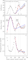 |
Fig. 5. Time-resolved (1 s bins) properties, with 1σ errors, of the thermonuclear X-ray burst observed from IGR J17591–2342 with AstroSat/LAXPC (see section 4.2.2). Parameter values of panels a, b, c are the same as panels c, d, e of Figure 2, respectively, and the vertical dotted lines mark the approximate maxima and minima of softness (panel a). The spectral parameter values of panels b and c were obtained by spectral fitting with the XSPEC model tbabs(bbodyrad+constant*powerlaw+gauss+gauss) and with powerlaw parameter values frozen to the pre-burst values (Section 3). In each panel, the blue best-fit model (solid line) does not include a Gaussian component for the hump, likely due to a second PRE, while the red best-fit model (solid line) includes such a component. An F-test between these two models shows the significance of the hump as likely being due to a second PRE (see Section 4.2.2). In panel c, the dotted red line is the solid red line minus its Gaussian component. Hence, a comparison between the solid and dotted red lines in panel c clearly shows the size of the blackbody temperature hump, which is likely due to a second PRE. |
4.2.3. Reliability of the simultaneous second radius hump and temperature dip: Robustness
Finally, we also suggest the robustness of (i) the second blackbody radius hump aligned with a kTBB dip and (ii) a subsequent kTBB peak aligned with a low radius value, as they do not depend on any of the following factors: (i) the evolution of the non-burst spectral shape during the burst, (ii) a specific pre-burst spectral model, (iii) whether the burst spectra are of 1 s or 2 s in duration, (iv) and the fitting of the excesses in the ∼6 − 8 keV and ∼12 − 20 keV ranges.
In order to show these, we created burst spectra for both 1 s and 2 s time bins and fit them with various reasonable models. First, we checked if the inclusion of a non-burst spectral shape evolution during the burst provides a better fit and affects the second radius hump signature. The upper panel of Figure 3 clearly shows that the burst data do not require a non-burst spectral shape evolution for the basic spectral model with only an absorbed blackbody and a power law. However, the fits for most spectra are unacceptable for this model due to high χν2 values.
From Figure 4, we find that the high χν2 values are due to the ∼6 − 8 keV and ∼12 − 20 keV excesses. Therefore, we included two Gaussians to describe these excesses in our updated spectral model (see Section 4.2). Thus, in order to test if the inclusion of a non-burst spectral shape evolution during the burst affects the second radius hump signature, we included these two Gaussians and allowed the non-burst spectral shape to evolve (see panels a1, a2, and a3 of Figure 6). When comparing this figure with Figure 2, for which the spectral model is the same except the non-burst spectral shape is frozen at the pre-burst value, we found that the χν2 values are generally not improved for the former. This suggests that a non-burst spectral shape evolution is not required by the burst data even when the excesses are fit with a suitable model, and thus the fits are acceptable.
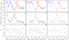 |
Fig. 6. Time-resolved properties, with 1σ errors, of the thermonuclear X-ray burst observed from IGR J17591–2342 with AstroSat/LAXPC (see section 4.2.3). The blackbody parameter (radius and temperature) and reduced χ2 profiles are shown for three cases: (i) fitting of 1 s burst spectra with the XSPEC model tbabs(bbodyrad+powerlaw+gauss+gauss) (panels a1, a2, a3); (ii) fitting of 1 s burst spectra with the XSPEC model tbabs(bbodyrad+constant*Nthcomp+gauss+gauss) (panels b1, b2, b3); and (iii) fitting of 2 s burst spectra with the XSPEC model tbabs(bbodyrad+constant*powerlaw+gauss+gauss) (the second Gaussian in ∼12 − 20 keV is included if required; panels c1, c2, c3). For (ii) and (iii), Comptonization (Nthcomp) and power-law parameter values were frozen to the pre-burst values (Section 3). This figure shows that the second blackbody radius hump aligned with a temperature dip is present for multiple reasonable models and spectra for different time bin sizes, and is thus robust. |
From panels a1 and a2 of Figure 6, we observed that the burst blackbody radius and temperature profiles are very similar to those for frozen non-burst spectral shapes (Figure 2), although as expected for the former, the error bars are larger. As before (see section 4.2.2), we fit the blackbody radius profile with a linear+Gaussian (χ2(d.o.f.) = 237.1(40)) and a linear+Gaussian+Gaussian (χ2(d.o.f.) = 43.3(37)). The results from an F-test imply that the second radius hump is ≈7.4σ significant. This shows that the second radius hump is not an artefact due to the freezing of the non-burst spectral shape during the burst.
The pre-burst spectrum can also be fit with a physical Comptonization model (XSPEC model Nthcomp), as mentioned in Section 3. Therefore, we fit the burst spectra with the XSPEC model tbabs(bbodyrad+constant*Nthcomp+gauss+gauss), where the Nthcomp parameter values were frozen to the pre-burst values. The burst blackbody radius and temperature profiles clearly show the signature of the second radius hump aligned with the temperature dip, and the χν2 values are similar to those for the XSPEC model tbabs(bbodyrad+constant*powerlaw+gauss+gauss) (see panels b1, b2, and b3 of Figure 6 and Figure 2). This suggests that the second radius hump and the aligned temperature dip do not depend on the specific model used to fit the pre-burst spectrum.
To check if the specific nature of the blackbody radius and temperature profiles depend on the 1 s duration of burst spectra, we made spectra for 2 s independent time bins during the burst, and we fit them with the XSPEC model tbabs(bbodyrad+constant*powerlaw+gauss+gauss) and with the power-law parameter values frozen to the pre-burst values (the second Gaussian in ∼12 − 20 keV is included if required; see panels c1, c2 and c3 of Figure 6). The χν2 values are similar to those for the 1 s burst spectra (compare with Figure 2). The blackbody radius and temperature profiles for the 2 s spectra clearly show the second radius hump and the aligned temperature dip, which do not depend on whether we use both Gaussians in the spectral model or, as required, only the one in ∼6 − 8 keV.
When comparing panels c1 and c2 of Figure 6 with the middle and lower panels of Figure 3, respectively, we found similar blackbody radius and temperature profiles and hence a clear signature of the second radius hump in both, although Gaussian models are not included for the latter figure. Therefore, the signature of the second radius hump, aligned with the temperature dip, is independent of the Gaussian models used to describe the ∼6 − 8 keV and ∼12 − 20 keV excesses.
Finally, we note that while the fast spin and the resulting oblateness of the neutron star could affect the obtained spectral parameter values by a few percent (Suleimanov et al. 2020), they cannot give rise to the humps and dips in the observed blackbody parameter profiles.
4.3. Model with spectral edge and an interpretation of evolving stellar atmospheric composition
Here, we fit the burst spectra with an alternative model for reasons explained below. We then compare its suitability relative to the spectral model described in Section 4.2.
We have shown that the burst blackbody radius (rBB/D10) profile for IGR J17591–2342 has a significant and robust second hump simultaneously with a blackbody temperature (kTBB) dip (see Sections 4.1, 4.2). From this, one could conclude the occurrence of a second PRE during the burst, assuming that the photospheric radius, r, and the effective temperature, kTeff, behave the same as rBB/D10 and kTBB, respectively. But, there is a way that rBB/D10 and kTBB could show such an anti-correlated behaviour, even when the photospheric radius, r, does not change; for example, the photosphere remains on the neutron star surface (r = R; R: stellar radius). This can be seen from Section 4.1. If r does not change, zr remains the same. Regardless, D10 is a constant for the source. Therefore, in this case,  . Thus, if fc temporarily decreases during a burst, the blackbody radius can temporarily increase, even if the photospheric radius r remains the same. A temporary decrease of fc can also temporarily reduce kTBB. On the other hand, if fc increases, RBB/D10 can decrease and kTBB can increase. Therefore, the signature of the second PRE, and even that of the first PRE, could result from a systematic evolution of fc.
We wished to identify what can cause a significant decrease and a subsequent increase of fc during one or more periods of a thermonuclear burst. This is possible if the metallicity of the neutron star atmosphere significantly increases and then decreases during such a period (Suleimanov et al. 2011; Kajava et al. 2017). To model such phenomena, one ideally needs to use realistic spectra of stellar atmospheres with various chemical compositions for a static, expanding, and contracting photosphere. There have been many efforts to compute realistic atmospheric spectra (e.g. London et al. 1986; Madej 1991; Suleimanov et al. 2011). However, a general atmospheric model with various compositions considering photospheric expansion is not yet publicly available for X-ray spectral fitting (e.g. using XSPEC). On the other hand, a diluted blackbody model with a parameter, fc, used to correct the measured photospheric radius and temperature usually fits the burst spectra well and is widely used (e.g. van Paradijs et al. 1990; Suleimanov et al. 2011; Keek et al. 2018; Suleimanov et al. 2020). We use this model in this paper. However, from this blackbody fitting it is not possible to discriminate between an atmosphere with evolving metal content (which should cause an fc evolution) and an expanding or contracting photosphere. Nonetheless, another way of inferring a metal content evolution is available. The spectrum from a metal-rich stellar atmosphere is typically expected to contain an absorption edge (around 7 − 10 keV) due to partially ionised Fe/Ni (e.g. Weinberg et al. 2006; in’t Zand & Weinberg 2010; Kajava et al. 2017; Li et al. 2018). Thus, one can test if the models used to fit observed burst spectra require such an edge.
Therefore, we examined our spectral results and performed additional spectral fits, including an absorption edge component, to critically analyse the alleged PREs. As previously mentioned, Figure 3 shows two periods of unacceptable fits during the burst for the basic model components, blackbody (for burst emission) and power law (for non-burst emission). These periods coincide with the blackbody radius humps, i.e. the alleged PREs. For both of these periods, unacceptable fits are due to unmodelled excesses in ∼6 − 8 keV and ∼12 − 20 keV (see Figure 4; only in ∼6 − 8 keV for some burst time bins). This similarity in spectra could indicate that the blackbody radius humps for both periods occur for the same reason–either an fc evolution due to a metallicity evolution or a photospheric expansion and contraction. After the excesses are fit with Gaussians, a spectral absorption edge is not required, indicating no significant metallicity of the stellar atmosphere. However, we wanted to know if these excesses could appear due to the lack of an absorption edge model component and not the absence of Gaussian components. Indeed, such a spectral edge component (without a Gaussian) could sufficiently improve the fit for bursts from other sources (Kajava et al. 2017; Li et al. 2018).
To test this, we fit the burst spectra with tbabs(edge*bbodyrad+constant*powerlaw). In this XSPEC model, the multiplicative component edge (absorption edge) as a function of energy (E) is 1 for E < Ec and exp[−D(E/Ec)−3] for E ≥ Ec. Here, Ec is the threshold energy and D is the absorption depth at the threshold2. The edge should originate from the neutron star atmosphere and hence is multiplied to bbodyrad (blackbody). Figure 7 compares the blackbody radius profiles and χν2 values during the radius humps between two cases: when the ∼6 − 8 keV and ∼12 − 20 keV excesses are modelled with an absorption edge and when they are modelled with Gaussian(s). We first found that the radius humps are qualitatively independent of the model component used to describe the excesses in the spectrum. This further shows the robustness of the second radius hump (see Section 4.2.3). Figure 7 also shows that during blackbody radius humps, the model including Gaussian(s) fits the burst spectra much better overall than the model including an absorption edge. For example, for the 2 s spectrum at the first blackbody radius peak (8 − 10 s since the burst onset), χ2(d.o.f.) ≈74.4(27) for the model including an edge. The probability (P) for a value drawn from the χ2 distribution to be equal to or higher than this obtained χ2 value for the given d.o.f. is ≈2.6 × 10⁻⁶. But, for the same spectrum and the model including Gaussian(s), χ2(d.o.f.) ≈28.2(23) and P ≈ 0.21. This shows that the model including Gaussian(s) provides a significantly better fit than the model including an edge.
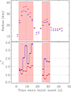 |
Fig. 7. Time-resolved properties, with 1σ errors, of the thermonuclear X-ray burst observed from IGR J17591–2342 with AstroSat/LAXPC (see Section 4.3). The upper panel shows the blackbody radius profiles for spectral fitting with the XSPEC models tbabs(bbodyrad+constant*powerlaw+gauss+gauss) (red; the second Gaussian in ∼12 − 20 keV is included if required) and tbabs(edge*bbodyrad+constant*powerlaw) (blue). The lower panel shows the reduced χ2 values for the same spectral models (marked in the same colours) for two phases of radius increase (highlighted in pink patches). The vertical dotted lines mark the approximate radius maxima. This figure shows that during the blackbody radius humps, the model including Gaussian(s) fits the burst spectra much better overall than the model including an edge, but the radius profiles are qualitatively the same for both models. |
For the two 2 s spectra at the second blackbody radius peak (26 − 28 s and 28 − 30 s since the burst onset), χ2(d.o.f.) ≈47.2(24) and ≈36.4(20), respectively, for the model including an edge. However, for these spectra, χ2(d.o.f.) ≈15.3(20) and 18.5(19), respectively, for the model including Gaussian(s). Since all of the 2 s spectra are for independent time bins, we added the χ2 values and d.o.f. values separately for the four spectra during the second blackbody radius hump (the second pink patch in Figure 7). For these four spectra, χ2(d.o.f.) ≈148.5(93) and P ≈ 0.0002 for the model including an edge, while χ2(d.o.f.) ≈86.9(83) and P ≈ 0.36 for the model including Gaussian(s). Therefore, although the observed flux during the second radius hump is much smaller than during the first radius hump, the two models can be identified during the second hump, and the model including Gaussian(s) fits significantly better. We note that if we combine the χ2 values and d.o.f. values separately for all 22 burst spectra of 2 s, we find χ2(d.o.f.) ≈894.5(559) and P ≈ 6.4 × 10⁻¹⁸ for the model including an edge and χ2(d.o.f.) ≈613.1(495) and P ≈ 0.0002 for the model including Gaussian(s). This suggests that the latter model fits the burst spectra significantly better overall than the former model.
To gain further insight, we also present the residuals of fits for the two models for the three above-mentioned burst spectra, one at the first blackbody radius peak and two at the second blackbody radius peak (see Figure 8). This figure clearly shows that a Gaussian can sufficiently fit the ∼6 − 8 keV excess, while an absorption edge cannot. Thus, an absorption edge cannot explain the burst spectra for either the first blackbody radius peak or the second radius peak. This implies that an atmospheric metallicity, and hence fc, evolution may not cause the blackbody radius humps. Therefore, these humps and the aligned blackbody temperature dips could be due to neutron star photospheric expansions.
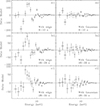 |
Fig. 8. Residuals (data−model) of fitting of the thermonuclear X-ray burst spectra (of 2 s time durations) observed from IGR J17591–2342 with AstroSat/LAXPC (see Section 4.3). Three spectra for 8 − 10 s (panels a1, a2), 26 − 28 s (panels b1, b2), and 28 − 30 s (panels c1, c2) since the burst onset are considered. These are times during the blackbody radius peaks. Left panels (a1, b1, c1) are for the XSPEC spectral model tbabs(edge*bbodyrad+constant*powerlaw), and right panels (a2, b2, c2) are for the model tbabs(bbodyrad+constant*powerlaw+gauss+gauss) (the second Gaussian in ∼12 − 20 keV is included if required). This figure shows that during the radius peaks, the model including Gaussian(s) fits the burst spectra better than the model including an edge does. |
5. Discussion and interpretation
In this paper, we have studied an unusual type-I X-ray burst from the neutron star X-ray binary and accretion-powered millisecond X-ray pulsar IGR J17591–2342. A detailed time-resolved spectroscopic investigation of the burst showed two significant and robust subsequent blackbody radius humps aligned with two blackbody temperature dips. This could be interpreted as two PREs during the same burst, or the second radius hump could be due to the neutron star atmospheric metallicity evolution. Each of these scenarios is extremely interesting. While the first one implies that a significant amount of fuel in the vicinity of the burning region of a powerful burst can remain unburnt, the second one could enable neutron star gravitational redshift measurement through observations of spectral lines. In the following, we compare the reliability of each scenario.
5.1. Discussion of the two scenarios
The second scenario, i.e. the neutron star atmospheric metallicity evolution, implies that a metal-rich stellar atmosphere should show an absorption edge component in the spectrum (around 7 − 10 keV) due to partially ionised Fe/Ni (e.g. Li et al. 2018). However, the fitting of burst spectra with the second model involving a spectral edge is clearly much worse compared to the first model involving reflection interpreted as a double PRE (see Section 4.3). Nevertheless, a metal-rich atmosphere without a strong edge is still plausible, for example, due to a relatively low Fe/Ni abundance. Therefore, while the occurrence of the first PRE is not unexpected, one cannot entirely rule out an atmospheric metallicity evolution origin of the second PRE signature.
Our results nonetheless favour a genuine PRE origin of the second blackbody radius hump, aligned with a temperature dip, for the following reasons. (i) Several previous papers predicted or found a spectral edge suggesting a metal-rich atmosphere (Weinberg et al. 2006; in’t Zand & Weinberg 2010; Kajava et al. 2017; Li et al. 2018), which we did not find. (ii) Spectral excesses in the ∼6 − 8 keV and ∼12 − 20 keV ranges during the burst blackbody radius humps indicate similar physical processes. Hence, a PRE origin of the first hump may suggest the same origin for the second hump. Otherwise, it is difficult to explain why there was a significant reflection off the disc during the first radius hump when the photosphere expanded and during the second radius hump when the photosphere did not expand but no significant disc reflection between the two radius humps when the photosphere did not expand. (iii) The lack of a spectral absorption edge during the first radius hump could suggest a metal-poor atmosphere with minimal or null enrichment even during a PRE event. Hence, coherently explaining a subsequent influx of metals sufficient to produce a second blackbody radius hump becomes difficult.
5.2. Burst flux evolution and its interpretation
Here, we present the flux evolution of the burst observed from IGR J17591–2342 and, considering the above observations, interpret this evolution assuming two PRE events during the burst (see section 4). For each 1 s burst time bin, we estimated the bolometric (0.01 − 100 keV) flux (FBB) of the burst blackbody (bbodyrad) component using the XSPEC cflux model (see panel f of Figure 2). We note that FBB relates to the luminosity at the observer by LBB = 4πD2ξFBB, where D is the source distance and ξ is the anisotropy factor due to mass distribution (e.g. accretion disc, Comptonizing hot electron gas) around the neutron star (e.g. Kuiper et al. 2020). On the other hand, the Eddington luminosity at the observer for a spherically symmetric burst emission is LBB, Edd = [4πGMc]/[0.2(1 + X)(1 + zR)] (e.g. Shapiro & Teukolsky 1983; Bult et al. 2019), where c is the speed of light in a vacuum and X is the fractional hydrogen abundance by mass in atmospheric layers. We note that a significantly asymmetric burning on the spinning neutron star would likely generate burst oscillations (Watts 2012), the lack of which suggests a spherically symmetric burst emission (see Appendices A and B). As shown in Figure 2, FBB first increased sharply within a second (consistent with Figure 1). Then it remained at a similar level for the first ∼20 s, when the first PRE occurred, but there is an indication of a dip at ∼10 s since the burst onset. We measured a maximum FBB of ≈7.5 × 10⁻⁸ erg s−1 cm−2 (note that Kuiper et al. 2020, reported a burst peak FBB of ∼7.6 × 10⁻⁸ erg s−1 cm−2 for their burst from this source). Finally, FBB decreased near-exponentially when the second PRE occurred.
Though LBB, Edd should correspond to the touchdown FBB (Damen et al. 1990; Ozel 2006), there are two widely different touchdown FBB values: ≈6.3 × 10⁻⁸ erg s−1 cm−2 for the first PRE event and ≈2.0 × 10⁻⁸ erg s−1 cm−2 for the second PRE event, implying a mismatch of a factor of ≈3. When equating LBB, Edd to LBB, we found that FBB can be different between the two touchdown points if X and/or ξ are different because FBB ∝ (1 + X)−1ξ−1. We note that X can range from 0 (pure helium) to 0.73 (cosmic abundance of hydrogen), which means that 1 + X could, in principle, explain a mismatch up to a factor of 1.73. A substantial increase in the anisotropy factor, ξ, between the two touchdown points should be accompanied by an irregular variation in the observed flux (Melia & Zylstra 1992). However, we observed a relatively smooth, near-exponential decay (Figures 1 and 2), similar to most other thermonuclear bursts. We note that it is unlikely that three largely independent parameters, kTBB, X, and ξ, evolved in a coordinated way to give rise to such a regular burst decay profile. Moreover, ξ could not have continued to increase monotonically from a value less than one (e.g. ξ = 1 implies isotropy; Kuiper et al. 2020). After its maximum value, ξ would have either decreased or remained the same, and hence, the burst decay profile should have abruptly become significantly less steep. Thus, X and ξ may not explain two widely different touchdown FBB values.
5.3. Discussion on the double-PRE scenario
Considering the double-PRE scenario, our analysis suggests the possibility of two novel and unexplained aspects of the thermonuclear type-I X-ray burst from IGR J17591–2342: (i) two PRE events occurring within a few seconds of each other and (ii) two touchdown luminosities (likely Eddington luminosities) different by a factor of roughly three (see Sections 4 and 5.2). Conscious of the theoretical challenge to explain two consecutive PRE events during the same type-I X-ray burst due to the need to preserve a significant amount of fuel sufficient to cause a second PRE event a few seconds after a strong burning with the first PRE, we briefly present a speculative, albeit reasonable, skeletal explanation for the puzzling findings mentioned above.
The sharp burst rise and subsequent PRE during a plateau-type FBB profile (see Section 5.2) strongly suggests an almost pure helium ignition and burning (e.g. Strohmayer & Bildsten 2006; Galloway et al. 2020; Bult et al. 2019; Jaisawal et al. 2019). However, the FBB plateau phase for a helium burst is usually much shorter (Strohmayer & Bildsten 2006) than the observed ∼20 s duration of this phase of the current burst, and indeed a previous thermonuclear burst observed from this source showed a plateau duration of ∼10 s (see Section 1). Combining this aspect with the previously mentioned dip in the flux profile ∼10 s after the burst onset and the long duration of the burst suggests a second step of energy generation, perhaps by subsequent thermonuclear burning of mixed hydrogen and helium stored at an upper layer (Fujimoto et al. 1988). Hydrogen in the upper layer is compatible with the evidence of the companion star being a hydrogen-rich low-mass star (Kuiper et al. 2020; Gusinskaia et al. 2020). However, it is unclear how this layer can remain unburnt during intense burning with the first PRE (Fujimoto et al. 1988; Spitkovsky et al. 2002). This question that may stimulate further detailed studies.
If the flux (FBB, td2) of the second touchdown point corresponds to LBB, Edd, then both PREs, during which the flux was higher (see Figure 2), could naturally occur. The remaining puzzle is then why the photosphere touched down on the stellar surface after the first PRE (∼20 s after the burst onset) when FBB was approximately three times FBB, td2. As shown earlier, evolutions of X and ξ cannot explain this puzzle, at least not entirely (Section 5.2). An explanation could come from the magnetic confinement of atmospheric layers if the stellar magnetic field is tangled and enhanced by convection at high luminosities (Boutloukos et al. 2010), which is compatible with the fact that IGR J17591–2342, being an AMXP, has a relatively higher magnetic field (Sanna et al. 2020; Tse et al. 2020). This convection could also mix helium in the atmosphere, thus decreasing X and increasing LBB, Edd and therefore helping the first touchdown. We note that as the burst luminosity decreased ∼20 s after the burst onset, perhaps helium largely subsided and the magnetic field tangling reduced, thus favouring the occurrence of the second PRE event.
Finally, the likely preservation of a substantial fuel mass in the vicinity of intense nuclear burning and a strong suggestion of magnetic confinement of plasma during thermonuclear fusion can challenge the current theoretical understanding (see e.g. Fujimoto et al. 1988; Spitkovsky et al. 2002). This could be interesting for multiple fields, such as plasma physics including a dynamo mechanism, supernova physics, and the nuclear, and particle physics of neutron stars, which involves strong gravity, high density, a large magnetic field, and intense radiation.
Acknowledgments
The authors acknowledge AstroSat Large Area X-ray Proportional Counter (LAXPC) teams (TIFR), Indian Space Research Organisation (including the Indian Space Science Data Centre), and the High Energy Astrophysics Science Archive Research Center (NASA/GSFC). The authors also thank H. M. Antia and T. Katoch (LAXPC team) for discussion on LAXPC pointing.
References
- Antia, H. M., Yadav, J. S., Agrawal, P. C., et al. 2017, ApJS, 231, 10 [NASA ADS] [CrossRef] [Google Scholar]
- Antia, H. M., Agrawal, P. C., Dedhia, D., et al. 2021, J. Astrophys. Astr., 42, 32 [Google Scholar]
- Ballantyne, D. R. 2004, MNRAS, 351, 57 [NASA ADS] [CrossRef] [Google Scholar]
- Bhattacharya, D., & van den Heuvel, E. P. J. 1991, Phys. Rep., 203, 1 [Google Scholar]
- Bhattacharyya, S. 2010, Adv. Space Res., 45, 949 [Google Scholar]
- Bhattacharyya, S. 2022, Astrophys. Space Sci. Libr., 465, 125 [Google Scholar]
- Bhattacharyya, S., & Strohmayer, T. E. 2006, ApJ, 642, L161 [Google Scholar]
- Bhattacharyya, S., & Strohmayer, T. E. 2007, ApJ, 666, L85 [Google Scholar]
- Boutloukos, S., Miller, M. C., & Lamb, F. K. 2010, ApJ, 720, L15 [NASA ADS] [CrossRef] [Google Scholar]
- Bult, P., Jaisawal, G. K., Guver, T., et al. 2019, ApJ, 885, L1 [CrossRef] [Google Scholar]
- Chakraborty, M., & Bhattacharyya, S. 2014, ApJ, 792, 4 [Google Scholar]
- Damen, E., Magnier, E., Lewin, W. H. G., et al. 1990, A&A, 237, 103 [NASA ADS] [Google Scholar]
- Fujimoto, M. Y., Sztajno, M., Lewin, W. H. G., & van Paradijs, J. 1988, A&A, 199, L9 [NASA ADS] [Google Scholar]
- Galloway, D. K., Muno, M. P., Hartman, J. M., Psaltis, D., & Chakrabarty, D. 2008, ApJS, 179, 360 [NASA ADS] [CrossRef] [Google Scholar]
- Galloway, D. K., in’t Zand, J., Chenevez, J., et al. 2020, ApJS, 249, 32 [NASA ADS] [CrossRef] [Google Scholar]
- Grindlay, J., Gursky, H., Schnopper, H., et al. 1976, ApJ, 205, L127 [NASA ADS] [CrossRef] [Google Scholar]
- Gusinskaia, N. V., Russell, T. D., Hessels, J. W. T., et al. 2020, MNRAS, 492, 1091 [CrossRef] [Google Scholar]
- Guver, T., Bostanci, Z. F., Boztepe, T., et al. 2022, ApJ, 935, 154 [CrossRef] [Google Scholar]
- in’t Zand, J. J. M., & Weinberg, N. N. 2010, A&A, 520, A81 [CrossRef] [EDP Sciences] [Google Scholar]
- Jaisawal, G. K., Chenevez, J., Bult, P., et al. 2019, ApJ, 883, 61 [NASA ADS] [CrossRef] [Google Scholar]
- Kajava, J. J. E., Nattila, J., Poutanen, J., et al. 2017, MNRAS, 464, L6 [NASA ADS] [CrossRef] [Google Scholar]
- Keek, L., Arzoumanian, Z., Bult, P., et al. 2018, ApJ, 855, L4 [NASA ADS] [CrossRef] [Google Scholar]
- Kuiper, L., Tsygankov, S. S., Falanga, M., et al. 2020, A&A, 641, A37 [NASA ADS] [CrossRef] [EDP Sciences] [Google Scholar]
- Lamb, D. Q., & Lamb, F. K. 1978, ApJ, 220, 291 [Google Scholar]
- Li, Z., Suleimanov, V. F., Poutanen, J., et al. 2018, ApJ, 866, 53 [NASA ADS] [CrossRef] [Google Scholar]
- London, R. A., Taam, R. E., & Howard, W. M. 1986, ApJ, 306, 170 [Google Scholar]
- Madej, J. 1991, ApJ, 376, 161 [NASA ADS] [CrossRef] [Google Scholar]
- Manca, A., Gambino, A. F., Sanna, A., et al. 2023, MNRAS, 519, 2309 [Google Scholar]
- Maqbool, B., Mudambi, S. P., Misra, R., et al. 2019, MNRAS, 486, 2964 [NASA ADS] [CrossRef] [Google Scholar]
- Melia, F., & Zylstra, G. J. 1992, ApJ, 398, L53 [Google Scholar]
- Miller, J. M. 2007, ARA&A, 45, 441 [NASA ADS] [CrossRef] [Google Scholar]
- Ozel, F. 2006, Nature, 441, 1115 [Google Scholar]
- Sanna, A., Ferrigno, C., Ray, P. S., et al. 2018, A&A, 617, L8 [NASA ADS] [CrossRef] [EDP Sciences] [Google Scholar]
- Sanna, A., Burderi, L., Gendreau, K. C., et al. 2020, MNRAS, 495, 1641 [Google Scholar]
- Seetha, S., & Kasturirangan, K. 2021, J. Astrophys. Astr., 42, 19 [Google Scholar]
- Shapiro, S. L., & Teukolsky, S. A. 1983, Black Holes, White Dwarfs, and Neutron Stars: The Physics of Compact Objects (John Wiley& Sons) [Google Scholar]
- Singh, A., Sanna, A., Bhattacharyya, S., et al. 2025, MNRAS, 536, 1323 [Google Scholar]
- Spitkovsky, A., Levin, Y., & Ushomirsky, G. 2002, ApJ, 566, 1018 [Google Scholar]
- Strohmayer, T. E., & Bildsten, L. 2006, in Compact Stellar X-ray Sources, eds. W. H. G. Lewin, & M. van der Klis (Cambridge: Cambridge University Press), 39, 113 [NASA ADS] [CrossRef] [Google Scholar]
- Strohmayer, T. E., & Markwardt, C. B. 2002, ApJ, 577, 337 [NASA ADS] [CrossRef] [Google Scholar]
- Strohmayer, T. E., Altamirano, D., Arzoumanian, Z., et al. 2019, ApJ, 878, L27 [NASA ADS] [CrossRef] [Google Scholar]
- Suleimanov, V., Poutanen, J., & Werner, K. 2011, A&A, 527, A139 [NASA ADS] [CrossRef] [EDP Sciences] [Google Scholar]
- Suleimanov, V. F., Poutanen, J., & Werner, K. 2020, A&A, 639, A33 [NASA ADS] [CrossRef] [EDP Sciences] [Google Scholar]
- Tse, K., Chou, Y., & Hsieh, H.-E. 2020, ApJ, 899, 120 [Google Scholar]
- van Paradijs, J., Dotani, T., & Tanaka, Y. 1990, PASJ, 42, 633 [Google Scholar]
- Walker, M. A. 1992, ApJ, 385, 642 [Google Scholar]
- Watts, A. L. 2012, ARA&A, 50, 609 [Google Scholar]
- Weinberg, N. N., Bildsten, L., & Schatz, H. 2006, ApJ, 639, 1018 [NASA ADS] [CrossRef] [Google Scholar]
- Worpel, H., Galloway, D. K., & Price, D. J. 2013, ApJ, 772, 94 [NASA ADS] [CrossRef] [Google Scholar]
Appendix A: A search for burst oscillations
We search for burst oscillations (see section 1) in the frequency range of 524 − 530 Hz (since the neutron star spin frequency is 527.43 Hz for IGR J17591–2342) and the energy range of ≈3 − 25 keV throughout the first 45 s of the type-I burst. We apply a sliding window search with window sizes of 1, 2, and 4 s (Bult et al. 2019) with a step of 0.1 s. Using the fractional amplitude maximisation technique (Chakraborty & Bhattacharyya 2014), which was shown to be similar to the Z2 power maximisation technique (Strohmayer & Markwardt 2002), we look for at least 3σ detection of burst oscillations in each time bin. Although a few time bins have better than 3σ detection, not even more than four consecutive and overlapping bins have ever had such a detection. Therefore, we consider these detections spurious. However, we estimate the upper limits of fractional root-mean-squared (rms) amplitude, which, for independent time bins of 1 s, comes out to be typically ∼3 − 4% for higher burst intensities and goes up to ∼13% in the burst tail.
Appendix B: A study of the burst rise
The 3 − 50 keV count rate during the burst from IGR J17591–2342 reached close to 6000 in the first ≈0.4 s, and exceeded 10000 in the first ∼1.3 s, which implies a drastic slope change of the intensity profile at ≈0.4 s since the burst onset. We perform a spectral fitting for the time period of ≈0.25 − 0.55 s since the burst onset, and find a blackbody bolometric (0.01 − 100 keV) flux FBB of ∼2.6 × 10⁻⁸ erg s−1 cm−2 using the XSPEC cflux model. This is more than the FBB value at the second touchdown point, which is ≈2.0 × 10⁻⁸ erg s−1 cm−2 (see panel f of Figure 2). Thus, the first PRE could have started within the first ∼0.4 s since the burst onset. Considering the first 1/3 s of the burst rise, we find the blackbody radius, temperature, bolometric flux, and the upper limit of the burst oscillation fractional rms amplitude to be  km,
km,  keV, ∼2.2 × 10⁻⁹ erg s−1 cm−2 and ∼33%, respectively. Since this temperature is already consistent with the peak temperature (see panel e of Figure 2), the burning timescale could be less than ∼1/3 s, supporting a pure helium or significantly hydrogen deficient burning (Strohmayer & Bildsten 2006) inferred in this paper. The low value of the blackbody radius suggests a localised ignition and that the thermonuclear flame had not yet spread all over the neutron star surface (section 1). A relatively high upper limit of the burst oscillation fractional rms amplitude during the first ∼1/3 s is consistent with this low value of the blackbody radius (and hence a small burning region). The low bolometric flux implies that the above-mentioned Eddington flux was not reached within the first ∼1/3 s. Thus, flame spreading and PRE perhaps happened simultaneously during the later part of the burst rise.
All Figures
|
Fig. 1. X-ray (3 − 50 keV) intensity versus time (with 0.1 s bins) of a thermonuclear type-I burst observed from the accreting millisecond X-ray pulsar IGR J17591–2342 with AstroSat/LAXPC (Section 2). |
| In the text | |
|
Fig. 2. Time-resolved (1s bins) properties with 1σ errors of the thermonuclear X-ray burst observed from IGR J17591–2342 with AstroSat/LAXPC. Panels a–c: Background-subtracted count rates in the energy range 3 − 6 keV, 12 − 15 keV, and their ratio, respectively. Panels d–f: Blackbody radius (rBB/D10), blackbody temperature kTBB, and bolometric (0.01–100 keV) blackbody flux FBB from the burst intervals best fits using the model tbabs(bbodyrad+constant*powerlaw+gauss+gauss) (see Sections 3, 4 and 5 for more details). The dotted horizontal line marks the FBB at the second touchdown point (see Section 5.2). Panel g: Reduced χ2 of spectral fits. |
| In the text | |
|
Fig. 3. Time-resolved (2 s bins) properties, with 1σ errors, of the thermonuclear X-ray burst observed from IGR J17591–2342 with AstroSat/LAXPC (see Section 4.1). The upper panel shows reduced χ2 profiles for the spectral fitting with the XSPEC models tbabs(bbodyrad+constant*powerlaw) (black; power-law parameter values frozen to the pre-burst values) and tbabs(bbodyrad+powerlaw) (red). This panel shows that the fitting is not acceptable. Overall, the fitting does not improve when the spectral shape (power-law photon index) is made free, and the reduced χ2 profiles have two humps. The middle and lower panels show the blackbody (bbodyrad) parameter (radius and temperature, respectively) profiles for the first model mentioned above. These panels (along with the dotted vertical lines) show that radius humps and temperature dips coincide with the reduced χ2 humps. |
| In the text | |
|
Fig. 4. Spectral fitting for the thermonuclear X-ray burst observed from IGR J17591–2342 with AstroSat/LAXPC (see Section 4.2). The spectrum is for 8 − 10 s since the burst onset, and the XSPEC model is tbabs(bbodyrad+constant*powerlaw) with the powerlaw parameter values frozen to the pre-burst values (Section 3). Upper panel: Unfolded spectrum. Data with 1σ errors are shown in red. The total model (solid histogram), tbabs*bbodyrad component (dashed line), and tbabs*constant*powerlaw component (dotted line) are also shown. Lower panel: Data-to-model ratio with errors. This figure shows that this model is not adequate because there are two excesses in the ∼6 − 8 keV and ∼12 − 20 keV ranges. |
| In the text | |
|
Fig. 5. Time-resolved (1 s bins) properties, with 1σ errors, of the thermonuclear X-ray burst observed from IGR J17591–2342 with AstroSat/LAXPC (see section 4.2.2). Parameter values of panels a, b, c are the same as panels c, d, e of Figure 2, respectively, and the vertical dotted lines mark the approximate maxima and minima of softness (panel a). The spectral parameter values of panels b and c were obtained by spectral fitting with the XSPEC model tbabs(bbodyrad+constant*powerlaw+gauss+gauss) and with powerlaw parameter values frozen to the pre-burst values (Section 3). In each panel, the blue best-fit model (solid line) does not include a Gaussian component for the hump, likely due to a second PRE, while the red best-fit model (solid line) includes such a component. An F-test between these two models shows the significance of the hump as likely being due to a second PRE (see Section 4.2.2). In panel c, the dotted red line is the solid red line minus its Gaussian component. Hence, a comparison between the solid and dotted red lines in panel c clearly shows the size of the blackbody temperature hump, which is likely due to a second PRE. |
| In the text | |
|
Fig. 6. Time-resolved properties, with 1σ errors, of the thermonuclear X-ray burst observed from IGR J17591–2342 with AstroSat/LAXPC (see section 4.2.3). The blackbody parameter (radius and temperature) and reduced χ2 profiles are shown for three cases: (i) fitting of 1 s burst spectra with the XSPEC model tbabs(bbodyrad+powerlaw+gauss+gauss) (panels a1, a2, a3); (ii) fitting of 1 s burst spectra with the XSPEC model tbabs(bbodyrad+constant*Nthcomp+gauss+gauss) (panels b1, b2, b3); and (iii) fitting of 2 s burst spectra with the XSPEC model tbabs(bbodyrad+constant*powerlaw+gauss+gauss) (the second Gaussian in ∼12 − 20 keV is included if required; panels c1, c2, c3). For (ii) and (iii), Comptonization (Nthcomp) and power-law parameter values were frozen to the pre-burst values (Section 3). This figure shows that the second blackbody radius hump aligned with a temperature dip is present for multiple reasonable models and spectra for different time bin sizes, and is thus robust. |
| In the text | |
|
Fig. 7. Time-resolved properties, with 1σ errors, of the thermonuclear X-ray burst observed from IGR J17591–2342 with AstroSat/LAXPC (see Section 4.3). The upper panel shows the blackbody radius profiles for spectral fitting with the XSPEC models tbabs(bbodyrad+constant*powerlaw+gauss+gauss) (red; the second Gaussian in ∼12 − 20 keV is included if required) and tbabs(edge*bbodyrad+constant*powerlaw) (blue). The lower panel shows the reduced χ2 values for the same spectral models (marked in the same colours) for two phases of radius increase (highlighted in pink patches). The vertical dotted lines mark the approximate radius maxima. This figure shows that during the blackbody radius humps, the model including Gaussian(s) fits the burst spectra much better overall than the model including an edge, but the radius profiles are qualitatively the same for both models. |
| In the text | |
|
Fig. 8. Residuals (data−model) of fitting of the thermonuclear X-ray burst spectra (of 2 s time durations) observed from IGR J17591–2342 with AstroSat/LAXPC (see Section 4.3). Three spectra for 8 − 10 s (panels a1, a2), 26 − 28 s (panels b1, b2), and 28 − 30 s (panels c1, c2) since the burst onset are considered. These are times during the blackbody radius peaks. Left panels (a1, b1, c1) are for the XSPEC spectral model tbabs(edge*bbodyrad+constant*powerlaw), and right panels (a2, b2, c2) are for the model tbabs(bbodyrad+constant*powerlaw+gauss+gauss) (the second Gaussian in ∼12 − 20 keV is included if required). This figure shows that during the radius peaks, the model including Gaussian(s) fits the burst spectra better than the model including an edge does. |
| In the text | |
Current usage metrics show cumulative count of Article Views (full-text article views including HTML views, PDF and ePub downloads, according to the available data) and Abstracts Views on Vision4Press platform.
Data correspond to usage on the plateform after 2015. The current usage metrics is available 48-96 hours after online publication and is updated daily on week days.
Initial download of the metrics may take a while.