| Issue |
A&A
Volume 701, September 2025
|
|
|---|---|---|
| Article Number | A56 | |
| Number of page(s) | 15 | |
| Section | The Sun and the Heliosphere | |
| DOI | https://doi.org/10.1051/0004-6361/202554105 | |
| Published online | 04 September 2025 | |
Solar wind speed maps from the Metis coronagraph observations
1
INAF – Torino Astrophysical Observatory, Via Osservatorio 20, I-10025 Pino Torinese, (TO), Italy
2
INAF – Catania Astrophysical Observatory, Via Santa Sofia 78, I-95123 Catania, Italy
3
INAF – Capodimonte Astronomical Observatory, Salita Moiariello 16, I-80131 Naples, Italy
4
Institute of Physics, University of Graz, Universitätsplatz 5, 8010 Graz, Austria
5
University of Firenze – Physics and Astronomy Department, Via Sansone 1, I-50019 Sesto Fiorentino, (FI), Italy
6
INAF – Arcetri Astrophysical Observatory, Largo Enrico Fermi 5, I-50125 Florence, Italy
7
Max-Planck-Institut für Sonnensystemforschung, Justus-von-Liebig-Weg 3, D-37077 Göttingen, Germany
8
INAF –Istituto di Astrofisica Spaziale e Fisica Cosmica, Via Alfonso Corti 12, I-20133 Milan, Italy
⋆ Corresponding author: This email address is being protected from spambots. You need JavaScript enabled to view it.
Received:
11
February
2025
Accepted:
21
July
2025
Abstract
Context. The solar wind plays a crucial role in shaping the heliosphere and influencing space weather. Understanding its origin and acceleration requires measurements of coronal dynamics. The Metis coronagraph on board of Solar Orbiter provides high-resolution simultaneous imaging of the middle solar corona in the polarized visible light and ultraviolet H I Lyα, which allows us to derive solar wind speed maps.
Aims. We determine solar wind speed maps by applying the Doppler dimming technique to Metis observations in the distance range from about 3.0 to 7.6 R⊙. The goal is to present the detailed algorithm, investigate the dependence of the speed on the parameters of the coronal model, and provide maps of the solar wind speed at the minimum of the solar activity. This is useful to improve our understanding of the physical processes that accelerate the wind.
Methods. Solar wind speeds are inferred by analyzing H I Lyα intensities in combination with electron density maps derived from visible-light polarized-brightness data. The Doppler dimming effect is used to estimate outflow velocities with different coronal model parameters, such as the electron temperature, the kinetic temperature, and the helium abundance, which are tested to assess their effect on the results.
Results. The wind speed maps confirm the bimodal distribution of the solar wind outflow velocities that characterize the near-minimum phases of solar activity. The slow wind (100−200 km s−1) confined to the equatorial streamer belt and fast wind (250−400 km s−1) originates from the polar coronal holes. The transition between these regions is sharp, with a steep velocity gradient at mid-latitudes. Variations in the coronal model parameters significantly affect the inferred speeds. This highlights the need for precise constraints on the coronal conditions.
Conclusions. Our method allows a systematic mapping of the solar wind speed and can be applied to data that are daily acquired by Metis throughout the current solar cycle. This provides new information on regions in which the wind is accelerated and on their evolution. These results provide valuable constraints for heliospheric models and theoretical studies of the formation of the solar wind. Future observations, in particular, during closer Solar Orbiter perihelia, will refine these measurements and improve our understanding of the solar corona and solar wind dynamics.
Key words: Sun: corona / solar wind / Sun: UV radiation
© The Authors 2025
 Open Access article, published by EDP Sciences, under the terms of the Creative Commons Attribution License (https://creativecommons.org/licenses/by/4.0), which permits unrestricted use, distribution, and reproduction in any medium, provided the original work is properly cited.
This article is published in open access under the Subscribe to Open model. This email address is being protected from spambots. You need JavaScript enabled to view it. to support open access publication.
1. Introduction
The study of the dynamic properties of the continuously expanding corona is important to gain insight into the origin of the solar wind and the creation of the heliosphere. The solar wind is a tenuous magnetized plasma that continuously escapes from the Sun into the interplanetary medium. It extends for thousands of millions of kilometers and is mainly characterized by a fast component, with typical velocities at 1 au of about 500−800 km s−1 that flows from coronal holes (CHs). Its slow component has typical velocities at 1 au of about 300−500 km s−1 and is mainly related to the streamer belt regions (see, e.g., Hundhausen 1972; Zirker 1977). It is important to study the solar wind for two main reasons: For its effect on the terrestrial environment, and for the basic physical processes of its formation and expansion.
Some strong lines in the UV spectral range observed in the solar corona up to several solar radii above the limb, for example, the H I Lyα at 121.6 nm and the O VI doublet at 103.2 and 103.7 nm, are very suitable for characterizing the properties of the solar wind in its early development. They are mainly excited by the disk radiation through the resonant scattering of incoming photons by the neutral atoms and ions in the corona, whereas the contribution from free-electron collisions is negligible because the outer solar atmosphere is highly rarefied (Gabriel 1971; Withbroe et al. 1982; Noci et al. 1987).
These spectral lines were extensively observed for the first time in the external atmosphere of the Sun with the UltraViolet Coronagraph Spectrometer (UVCS; Kohl et al. 1995) on board the SOlar and Heliospheric Observatory (SOHO; Domingo et al. 1995). UVCS allowed the discovery of fundamental properties of the proton and oxygen components of the solar wind (Kohl et al. 1997; Raymond et al. 1997; Noci et al. 1997). Coronal outflows were detected out to about 5−6 R⊙ with spectroscopic techniques that are based on the Doppler dimming of the resonantly scattered UV light emitted by coronal ions and atoms (see, e.g., Withbroe et al. 1982; Noci et al. 1987). In a region with solar wind flow, the disk line profile is Doppler shifted (redshifted) with respect to the coronal scattering profile. The resulting weaker scattering reduces the intensity of the scattered radiation, which decreases as the flow velocity increases. The main UVCS results on the solar wind include the measurement of the outflow speed in the coronal hole and streamer regions and the observational evidence of energy deposition in the coronal hole regions (e.g., Kohl et al. 1998; Cranmer et al. 1999; Giordano et al. 2000; Strachan et al. 2002; Spadaro et al. 2007; Susino et al. 2008), which was reported in several reviews in the past decade (e.g., Antonucci et al. 2012, 2020a; Abbo et al. 2016; Cranmer et al. 2017; Cranmer 2020; Kohl et al. 2006).
The UVCS allowed us to detect the H I Lyα light at a very high spatial and spectral resolution, but in a narrow instantaneous field of view (FOV). Therefore, maps of the neutral hydrogen atoms line emission in the corona could only be reconstructed under the hypothesis of steady conditions, from data that were collected at different times and without a continuous spatial coverage of a given annulus of the corona (see, e.g., Dolei et al. 2018). On the other hand, Dolei et al. (2018, 2019) showed that the simultaneous availability of UV Lyα and visible-light polarized-brightness images of the solar corona can enable us to derive global maps of the H I outflow velocity in the inner heliosphere. In addition to UVCS data, they also used visible-light observations acquired by the Large Angle and Spectrometric COronagraph (LASCO; Brueckner et al. 1995) on board SOHO. Because protons and neutral hydrogen atoms are closely coupled in the regions of the solar corona below approximately 10 R⊙, where the time for hydrogen-proton charge exchange is shorter than the coronal expansion time (e.g., Olsen et al. 1994; Allen et al. 1998), the H I outflow velocity maps also give information on the global dynamics and evolution of the proton component in the solar atmosphere. This component carries most of the mass of the solar wind and thus represents the main component of the coronal plasma.
The purpose of widening the knowledge that was previously acquired with UVCS led to the design of the Metis coronagraph (Antonucci et al. 2020b; Fineschi et al. 2000, 2020) on board the Solar Orbiter mission (Müller et al. 2020). Metis is able to simultaneously image the full off-limb corona at a high temporal and spatial resolution in the polarized visible light (VL) in the band 580−640 nm, and in the ultraviolet (UV) H I Lyα line narrow-band (121.6 ± 10 nm) for this first time. This provides an unprecedented view of the solar wind acceleration region over a wide range of heliocentric distances from 1.7 to 9 R⊙, depending on the distance of the spacecraft from the Sun.
This combination of data can indeed probe the speed of the expanding coronal plasma, as was shown by Romoli et al. (2021) and Antonucci et al. (2023). These authors specifically used the first observations performed by Metis to obtain the first instantaneous map of the speed of the coronal plasma outflows in the equatorial streamer belt during the minimum of solar activity. They only examined the interval at ±30° latitude across the solar equator. Moreover, Telloni et al. (2021, 2023) determined the radial profile of the neutral hydrogen outflow velocity at equatorial and polar latitudes based on data that were acquired during the first quadrature of Solar Orbiter with Parker Solar Probe (PSP; Fox et al. 2016).
We illustrate the physical bases and the computational techniques for determining the solar wind speed maps from the data acquired with Metis in detail. We also describe the dependence of the results on the coronal model parameters that were studied over a wide grid of possible values. Then we present some solar wind speed maps, which cover the full latitudinal range in the solar corona. We show in particular the maps that were obtained from a set of Metis data that were collected during the cruise phase of the Solar Orbiter mission. This phase was soon after the first perihelion at about 0.5 au in June 2020, and before and after the second perihelion at about 0.5 au in January and February 2021. These maps can provide a means for obtaining information on the outward flow velocities, as well as on the mass flux, as a function of height above the solar limb and latitude. This results in a sensitive determination of the magnitude and location of the solar wind acceleration near the Sun, which is useful for locating and characterizing the source regions of the coronal solar wind and for identifying and understanding the dominant physical processes that accelerate it.
2. H I Lyα formation in the corona
The H I Lyα photons at λ0 = 121.6 nm from the lower solar atmosphere are absorbed by neutral hydrogen atoms in the corona. This causes a quantum jump in the electron from the ground state (n = 1, where n is the principal quantum number) to the immediately higher energy level (n = 2). The subsequent spontaneous (2p−1s) transition to the fundamental level produces the H I Lyα line that is observed in the extended corona. Even though only about one proton in 107 is tied up in neutral hydrogen at coronal temperatures and densities, the large coronal proton abundance coupled with the high intensity of the chromospheric Lyα radiation gives rise to a resonantly scattered coronal component of Lyα that is strong enough to be measured out to large distances above the solar surface (Gabriel 1971).
The intensity of the coronal H I Lyα line depends on the number of particles in the line of sight that are able to scatter radiation in the line, that is, it depends on the local state of the coronal plasma (neutral atom density, nHI, electron temperature, Te, and neutral atom kinetic temperature, Tk) and on the intensity and profile of the incoming radiation from the solar disk and lower levels of the corona. Incident Lyα photons from a direction n′ are distributed around the line rest wavelength λ0 according to the chromospheric profile, I(λ, n′). The velocity distribution function f(v) of hydrogen atoms depends on the kinetic temperature Tk of the neutral atom and sets the coronal Lyα absorption profile, Φ(λ, n′,Tk).
The number of scatterings also depends on the outflow velocity of the solar plasma, vout. In a static atmosphere, the central wavelength of the line profile of the coronal scattering is identical to the wavelength of the disk profile. In a region with solar wind flow, however, the Lyα disk profile is Doppler shifted (redshifted) with respect to the coronal scattering profile (see Fig. 1). The weaker scattering results in a weaker scattered radiation that decreases as the flow velocity increases. This effect is known as Doppler dimming (see Hyder & Lites 1970; Beckers & Chipman 1974).
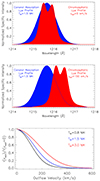 |
Fig. 1. Top panel: Chromospheric Lyα profile (red) and coronal absorption Lyα profile (blue) for a static corona (vout = 0 km s−1). Middle panel: Chromospheric and absorption profiles Doppler shifted for an outflow velocity of 150 km s−1. The absorption coronal profile is calculated as a Gaussian shape for a neutral hydrogen kinetic temperature equal to 1.5 MK. Bottom panel: I(vout)/I(vout = 0) calculated for three different neutral hydrogen kinetic temperatures, Tk = 0.8 MK (black), Tk = 1.5 MK (blue), and Tk = 3.0 MK (red). |
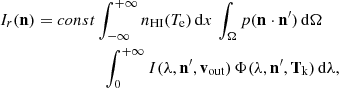
As shown in Fig. 1 (bottom panel), the Lyα line is significantly weaker than the static conditions for outflow velocities higher than 80 km s−1 and it appears to be almost completely dimmed for vout ≥ 400 km s−1 because the excitation and absorption profiles are completely Doppler shifted from each other. The corona therefore becomes invisible at the wavelength of 121.6 nm. The techniques for computing the amount of Doppler dimming were described by Kohl & Withbroe (1982), Withbroe et al. (1982), Noci et al. (1987). The resonance between the incident chromospheric profile,  , in the direction n′ and the coronal absorption profile determines the intensity Ir(n) (in units of photons cm−2 s−1 sr−1) of the H I Lyα line that is emitted toward an observer in the n direction, according to the simplified expression (see, e.g., Withbroe et al. 1982; Noci et al. 1987)
 (1)
(1)
where x is the spatial coordinate along the line of sight, the function p(n ⋅ n′) expresses the angular dependence of the Lyα scattering process, and Ω is the solid angle under which each point along the line of sight subtends the solar disk (see Fig. 2). For the outflow velocity in Eq. (1), we used the vector notation vout because the process depends on the angle between the direction of the incident radiation n′ and the wind velocity, which is hereafter assumed to be radial. A detailed description of the equations, geometry, and computation procedures we adopted for this is reported in the appendix.
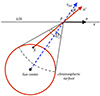 |
Fig. 2. Simplified geometry of the radiation from the chromospheric point S, resonantly scattered in the coronal point P at the heliocentric distance r. The x-axis represents the line of sight of the observer, vout is the outflow velocity, which we assumed to be radial, and Ω is the solid angle subtended by the point P. The vectors n′ and n give the directions of the incident and scattered photons, respectively. |
3. Metis observations and data reduction
The Metis data we analyzed were collected on June 21, 2020, January 14–17, 2021, and February 12–19, 2021, during the first part of the Solar Orbiter cruise phase and near its first two perihelion passages, which occurred on June 15, 2020, and February 10, 2021, at heliocentric distances of 0.52 and 0.49 au, respectively, when the spacecraft was near the solar equatorial plane. At that time, which corresponds to the very beginning of the current solar cycle, the global configuration of the corona was that typical of a solar minimum. It was characterized by a quasi-dipolar magnetic field topology with a bright equatorial streamer belt in which the coronal/heliospheric current sheet was embedded and that separated the two large open-field regions that are located above the solar poles.
The three datasets we considered consist of simultaneous visible-light and UV Lyα images acquired in the two Metis passbands at a constant cadence. In visible light, in particular, we acquired sequences of polarized images at the four polarization angles of 0°, 45°, 90°, and 135° to retrieve the intensity of the total (B) and linearly polarized (pB) components of the Thomson-scattered K-corona.
In all three cases, observations were aimed at studying the long-term evolution of the overall coronal configuration, and the spatial resolutions, exposure times, and cadences were therefore optimized to address this objective. The complete set of observational parameters we used in the three datasets is listed in Table 1, along with the spacecraft position, given in terms of its distance from the Sun, D⊙, and its longitude relative to the Earth view, L0.
Observational parameters.
To increase the signal-to-noise ratio and enhance data statistics, observations were performed by averaging several consecutive frames that were acquired with the same exposure time, as reported in the Table 1. For the visible-light observations, single frames were also acquired by cycling over the four polarization angles, and averages were made between frames with the same polarization state. As a consequence, the effective time over which the coronal signal was integrated was longer than the single-frame exposure time and equal to ∼1200 s for the two channels in June 2020 and to ∼1800 s and 900 s for the visible-light and UV channels, respectively, in January and February 2021. In the latter cases, two UV images were acquired in parallel with each visible-light pB sequence.
In addition, a spatial binning of 4 × 4 pixel2 (in June 2020) and 2 × 2 pixel2 (in January and February 2021) was applied during the observations. Since the nominal plate scales of Metis detectors are 10.14 arcsec/pixel for the visible-light channel and 20.4 arcsec/pixel for the UV channel, the corresponding spatial elements on the Metis plane of the sky were ∼16 000 km/pixel (in June 2020) and ∼8000 km/pixel (in January and February 2021) for the visible-light channel and nearly twice this for the UV channel with the above binning and for the distances at which Solar Orbiter observed.
The data were calibrated with standard operations, including detector bias and dark-current subtraction, correction for flat-field and optical vignetting, and exposure-time normalization (see Romoli et al. 2021). In the case of the UV images, an additional dark-current correction was performed to address a known issue of the Metis UV camera that consists of transient variations in the detector response (Uslenghi et al. 2024). The most recent radiometric calibration (see De Leo et al. 2023, 2025) was applied to convert the count rates into physical units. For the UV channel, this also included a spatial correction of the optical vignetting function that was needed to fix the significant nonuniformity of the detector efficiency, which was detected in the analysis of several calibration-star transits in the Metis FOV (see Andretta et al. 2021; Russano et al. 2024; De Leo et al. 2025, for further details). Finally, each set of four polarized visible-light images was combined by demodulation based on the Müller formalism (see Liberatore et al. 2023) to obtain total and polarized-brightness coronal images.
To address the discrepancies between the Metis and LASCO C2 pB measurements that were recently highlighted by Vásquez et al. (2025), we thoroughly revised all steps of the radiometric calibration of the Metis VL channel, as originally described by De Leo et al. (2023). This revision also included a reassessment of the calibration data derived from the on-ground campaign, specifically, the vignetting function and its normalization. The reanalysis of the flight calibration data led to a correction of 18% in the application of the vignetting function. Since the UV channel vignetting function is derived from that of the VL channel (see De Leo et al. 2025), this correction likewise applies to the calibration of the UV channel as derived by De Leo et al. (2025). In addition, an inaccuracy in the VL channel of 19% was found in the value of the zeropoint Johnson R magnitude definition used by De Leo et al. (2023) (see Table A.2 of Bessell et al. 1998).
Consequently, the VL radiometric calibration coefficient reported by De Leo et al. (2023) must be multiplied by a factor of 1.18 (from the vignetting correction) and 1.19 (from the zeropoint Johnson R magnitude correction). This yields a total correction factor of 1.40. The UV radiometric coefficient reported by De Leo et al. (2025) must be multiplied by 1.18. As a result, the visible-light pB and H I Lyα intensities derived from Metis data using the radiometric calibration described by De Leo et al. (2023, 2025) should be corrected by a division by factors of 1.40 and 1.18, respectively. A detailed account of the updated Metis radiometric calibration will be the argument of a forthcoming publication.
Figure 3 shows the two maps of visible-light pB and H I Lyα intensity derived from Metis data acquired on January 14, 2021, between 00:30 and 01:00 UT as an example. To further increase the signal-to-noise ratio, the Lyα intensity map was obtained by averaging the two UV images acquired in parallel with the polarized sequence that was used to derive the pB map. The two maps were used in the following as a test case for the application of the Doppler dimming technique and to discuss the results.
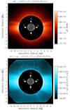 |
Fig. 3. Simultaneous maps of visible-light pB (top panel) and H I Lyα intensity (bottom panel) from the Metis observations performed on January 14, 2021, at 00:45 UT. The solar disk was detected in both images at 00:45 UT by the EUI instrument on board the Solar Orbiter at a wavelength of 171 A (gray scale) and was superimposed in the center. |
In both channels, the coronal emission is mainly concentrated in the equatorial streamer belt, where the coronal/heliospheric current sheet that separates the two regions of opposite magnetic polarity that are located over the poles (dipolar configuration) is likely to form, as expected during near-minimum levels of the solar activity. While the streamer above the east limb exhibits the characteristic cusp shape typical of equatorial streamers at solar minimum, the streamer above the west limb appears to be more diffuse and is characterized by several thin radial features that are clearly evident in the visible light between ∼40°S and 30°N. This hinders a firm identification of the position of the heliospheric current sheet.
In both cases, however, the transition between the equatorial streamer belt and the surrounding regions is quite sharp, with a steep drop in coronal emission at higher latitudes in the two Metis passbands. This is evidenced by the latitudinal distribution of the emission at two representative heights in the corona, as shown in Fig. 4.
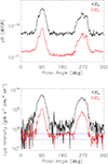 |
Fig. 4. Latitudinal distributions of the visible-light pB (top panel) and H I Lyα intensity (bottom panel) at 4.0 and 6.0 R⊙, derived from the maps shown in Fig. 3. The latitude is expressed in terms of the polar angle, measured counterclockwise from the north pole. In the bottom panel, the horizontal dashed blue lines mark the expected range of the H I Lyα interplanetary emission (3 − 6 × 10⁷ photons s−1 cm−2 sr−1; see, e.g., Kohl et al. 1997; Akinari 2007). |
In the equatorial streamers, the pB is higher by at least five times than in the adjacent regions, and the decrease occurs in an angular interval of ∼30° around the equatorial plane. In the west streamer, several secondary peaks in the brightness profile mark the positions of the ray-like features that are visible in the pB map, as mentioned above. Outside the streamers, the level of pB is then nearly uniform and fluctuates very little. This might be ascribed to either thin coronal structures such as polar plumes or to data noise. The latitudinal trend is very similar at the two considered heights of 4 and 6 R⊙. The level of pB at the higher altitude is approximately four times lower.
The H I Lyα intensity exhibits the same latitudinal distribution as the visible light, but we note that the higher level of noise affects the line intensities in the polar regions, where the Lyα emission is lower by at least one order of magnitude than in the equatorial regions. Moreover, around 6 R⊙, the observed line intensities are comparable with the values expected for the interplanetary H I Lyα emission (Kohl et al. 1997; Akinari 2007), so that the source of the detected photons may not be the considered coronal polar regions.
It is worth noting that the main source of uncertainty in the data arises from the radiometric calibration process. According to De Leo et al. (2023, 2025), and Liberatore et al. (2023), the errors in the radiometric factors of the VL and UV channels of Metis are about 7% and 15%, respectively. We estimated that the overall uncertainties affecting the measured intensities, including bias/dark subtraction, vignetting correction, and radiometric calibration, are about 10% and 20% on average for the two channels, respectively. We adopted these values to estimate the errors in the electron density and outflow velocity determination, as described in the following sections.
4. Data analysis
Spectroscopic observations of the UV solar corona and measurements of the intensity of the H I Lyα in particular can thus be used in conjunction with visible-light observations of the coronal polarized brightness to probe the speed of the expanding coronal plasma. The outflow velocity in the solar corona is generally derived by comparing the observed resonantly scattered H I Lyα emission and the synthetic emission calculated by Eq. (1), adopting a suitable set of values of the physical parameters described in Sect. 4.2 and in the appendix, as input data in the synthesis computation (see, e.g., Romoli et al. 2021; Antonucci et al. 2023). The density of the coronal scattering neutral atoms, nHI, is computed as a function of the electron density, ne, derived from the observed polarized brightness (see Sect. 4.1), after adopting a value for the coronal helium abundance and for the assumed electron temperature. The calculated intensity depends on the only free parameter, the outflow velocity, whose value is returned iteratively until a satisfactory match (e.g., within 1%) between the calculated and observed intensities is reached. We describe the algorithms that determine the outflow velocity and the related numerical tools we adopted in more detail below.
4.1. Electron density maps
The maps of pB obtained by Metis were used to derive electron density maps by means of the inversion technique that was initially developed by van de Hulst (1950), assuming cylindrical symmetry for the solar corona (see, e.g., Antonucci et al. 2020b). The inversion procedure requires fitting the radial trend of pB with a power law. Therefore, the images were first converted from rectangular (x, y) into polar (r, θ), coordinates, with a fixed resolution in the radial and latitudinal directions. We chose dr = 0.01 R⊙, and dθ = 1°. All the results presented here were obtained with this resolution. The electron density map derived from the pB map reported in Fig. 3 (top panel) is shown in Fig. 5, and two electron density latitudinal profiles we obtained for heliocentric distances equal to 4.0 and 6.0 R⊙, respectively, are reported in Fig. 6. The electron density values are affected by uncertainties of about 10% that take the pB measurement errors estimated in Sect. 3 into account. The latitudinal distribution of the electron density clearly shows the characteristic configuration of the solar corona during the near-minimum phase of solar activity, when the global-scale magnetic field is predominantly dipolar and confines the plasma mostly near the equator, giving rise to a quasi-equatorial streamer belt. The polar regions, conversely, exhibit a significantly lower density.
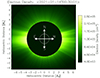 |
Fig. 5. Electron density map from Metis pB observations performed on January 14, 2021, at 00:45 UT. |
4.2. Doppler dimming technique. Inversion method for determining the outflow speed
To compute the expected H I Lyα emission from the solar corona, we started by setting the intensity and spectral profile of the incoming chromospheric radiation. The Lyα irradiance increases by up to about a factor of 2 from the minimum to the maximum of the solar cycle, and it varies in a time range of a few days by less than 5% at solar minimum and up to 20% during the maximum of solar activity (Machol et al. 2019). Because we cannot have the daily value of the radiation as seen from the scattering atom, we adopted for each set of Metis observations the chromospheric intensity as that computed from the ±7-day average irradiance values available by the LASP Interactive Solar IRradiance Datacenter (LISIRD1). In the case studies presented here, we used the chromospheric intensities listed in Table 2.
Chromospheric intensity from ±7-day average irradiance values.
We assumed a uniform distribution of the Lyα brightness over the solar disk. Dolei et al. (2019) investigated the dependence of the derived outflow velocities on the chromospheric H I Lyα brightness distribution. They found that the uniform-disk approximation systematically leads to an overestimated velocity in the polar and mid-latitude coronal regions of up to some tens of km s−1 closer to the Sun. It also leads to slightly underestimated velocities at equatorial latitudes. These differences decrease at higher heliocentric distances, where an increasingly larger chromospheric portion, including brighter and darker disk features, contributes to illuminating the solar corona, and the nonuniform radiation condition progressively approaches the uniform-disk approximation.
The chromospheric line profile is represented by the analytic function reported by Auchère (2005) and was assumed to be uniform over the solar disk because it was proved that the nonuniformity of the shape of the H I Lyα line profile observed in the chromosphere does not induce remarkable effects on the estimate of the outflow velocity (Capuano et al. 2021).
The total Lyα intensity computation required a full 3D description of the following physical coronal parameters: the electron density, ne, electron temperature, Te, the kinetic temperature, Tk, the kinetic temperature anisotropy, Ki, the helium abundance, AHe, and the outflow speed, vout. For all of these parameters, the data volumes were constructed under the assumption of cylindrical symmetry around the north–south rotation axis. For each point in the plane of the sky, the value of each individual element along the line of sight solely depends on its heliocentric distance under this assumption. This is consistent with the radial variation determined for electron density or assumed, as in the case of electron temperature, on the plane of the sky. The parameter volumes covered heliocentric distances from the minimum, rmin, to the maximum observed distance, rmax, in the plane of the sky, and extended to 2 rmax along the line of sight. In this way, we accounted for the contribution to the total intensity of plasma elements far from the plane of the sky, which can be significant at large heliocentric distances where the decrease in the electron density with distance from the Sun is weaker. We verified that for maximum observed distances of about 8 solar radii, considering a line of sight length greater than twice the maximum observed distance results in negligible contributions to the calculated total intensity.
The electron density, as discussed in the previous section, was determined from the measurements pB and extrapolated at heliocentric distances larger than those observed by using the radial profile from Leblanc et al. (1998).
Because the electron temperature is not measured, we needed to perform the computation under different assumptions, that is, setting different constant values, which ranged from 0.4 to 1.6 MK. Alternatively, we adopted the radial profiles determined by Gibson et al. (1999) and Vásquez et al. (2003), which are reported in Fig. 7.
The kinetic temperature of neutral hydrogen scattering atoms, Tk, is a parameter that has to be assumed on the basis of Lyα line widths measured from UVCS/SOHO spectroscopic observations of streamers as well as of coronal holes (e.g. Cranmer et al. 1999; Antonucci et al. 2000; Dolei et al. 2016), which suggest a range from 1.0 to 3 MK for coronal streamers and from 1.0 to 2 MK for coronal holes. In this range, we therefore determined the wind speed for a grid of constant coronal kinetic temperatures.
The distribution of the kinetic temperature can be isotropic, that is, the same temperature value is assumed in all directions, or anisotropic, that is, the value of the temperature in the direction perpendicular to the magnetic field lines, T⊥ is assumed to be different from that in the parallel direction, T||. For this reason, we defined the anisotropy factor as  . In the outer corona above 2.5 R⊙, the direction of the magnetic field can be considered to be almost radial, so that the value of T⊥ actually corresponds to the kinetic temperature derived from the observed line profile widths, while
  sets the width of the coronal neutral hydrogen absorption line profile used for the synthesis of the Lyα line intensity.
The anisotropic distributions studied in the case of heavy ions with UVCS coronal spectroscopic observations (Dodero et al. 1998; Cranmer et al. 1999), typically show values of Ki up to about 10 (e.g. Kohl et al. 1998; Cranmer et al. 1999), which have been interpreted as the signature of ion cyclotron resonance coronal heating mechanisms. For neutral hydrogen atoms, there is evidence that lower anisotropy factors do not exceed values of approximately 2 (Susino et al. 2008; Cranmer 2020). We explored the effect of different assumptions on the anisotropy factor in the range from Ki = 1 to Ki = 2 for different kinetic temperatures. In addition, recent observational and theoretical studies, such as those quoted by Cranmer (2020), pointed out that the neutral hydrogen kinetic temperature is greater than or equal to that of electrons.
The helium abundance based on which the neutral hydrogen density is derived from the electron density map (see Eq. A.3 in the Appendix) is generally adopted to be equal to 10% (see, e.g., Withbroe et al. 1982). On the other hand, recent measurements performed by Moses et al. (2020) found helium abundance values as low as 2.5% in the core of the equatorial coronal streamer observed by SCORE/HERSCHEL (Fineschi et al. 2003) at solar minimum activity.
In Table 3 we summarize the quantities required to perform the Doppler dimming analysis and to derive the solar wind speed. Since some components of the model are only poorly constrained, we explored the space of physically acceptable parameters; the table also provides estimates of their impact on the derived speeds. A detailed analysis of the dependence of the inferred wind speed on the assumed parameters is presented in Section 5.
Computation parameters and effect on the wind speed determination.
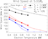 |
Fig. 11. Computed solar wind speed as a function of electron temperature at 5 R⊙ for different latitudes (polar: black, mid: red, and equatorial: blue) and with two different assumptions on the kinetic temperature: Tk = 1.0 MK (full line and circles) and Tk = 2.0 MK (dashed line and open circles). |
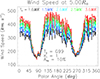 |
Fig. 12. Computed solar wind speed as a function of latitude at 5 R⊙, adopting the electron temperature profile from Gibson et al. (1999) and with five different assumptions on the kinetic temperature. |
After we assumed the intensity and spectral profile of the incoming chromospheric radiation, a temperature and abundance model of the corona, and an arbitrary speed of the solar wind, we calculated the synthetic intensity of coronal H I Lyα at a fixed point on the plane of the sky (POS) by integrating the emissivity along the corresponding line of sight (LOS). The profiles of the physical corona parameters along the LOS, in particular, the electron density as well as the temperatures, were determined by adopting an extrapolation of the radial profiles measured or assumed on the POS.
The outflow speed is the parameter that is to be determined. It was initially set to a value of 0 km s−1 and was left as a free parameter to vary up to 600 km s−1 in order to determine the 1% agreement between the synthetic and observed intensity in each image pixel. The outflow speed derived using the described diagnostic method is representative of the velocity projected onto the plane of the sky.
An initial solar wind speed map was obtained by assuming a constant speed along the LOS for each spatial element in the plane of the sky. In a second iteration over all spatial elements, we then recalculated the intensity of H I Lyα and compared it with the observed values by adopting a speed profile along the LOS. These profiles were defined for each radial direction and were derived from a monotonic fit to the radial speed distribution obtained from the initial image. In this way, the LOS contributions were treated more realistically, under the assumption that the outflow speed increases with heliocentric distance.
A more detailed description of the solar corona can be used to resolve the structure of the solar wind outflows at a finer level, as was done by Antonucci et al. (2023) in their analysis of the Metis first-light observations. The functional dependence along the LOS of the electron density that is taken into account in the Lyα line emissivity calculation was the dependence that was returned by a 3D magnetohydrodynamic model of the global corona developed by Predictive Science Inc. (MAS, Lionello et al. 2009; Mikić et al. 2018), considering the position of Solar Orbiter with respect to the Sun at the time of the Metis observations. This approach is beyond the purposes of this work, however, which aims to present solar wind speed maps that can be derived from a single pair of pB and H I Lyα images using the fewest possible assumptions on the coronal model.
The top panel of Fig. 8 shows the velocity map obtained from the H I Lyα line intensity and visible-light pB maps reported in Fig. 3 as a representative example of the results obtained by the procedure described above. Some related latitudinal velocity profiles are also shown in Fig. 9, to help us discuss this result. This velocity map was obtained by adopting the temperature radial profile given by Gibson et al. (1999) (see Fig. 7) at all latitudes, a constant kinetic temperature of 1 MK with isotropic kinetic temperature distribution, Ki = 1, and a helium abundance of 10% with respect to hydrogen.
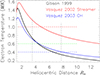 |
Fig. 7. Electron temperature radial profile from Gibson et al. (1999) (black), Vásquez et al. (2003), coronal hole (blue), and streamer (red). The vertical dashed lines show the range of the field of view observed by Metis on January 14, 2021, and the horizontal dashed lines represents the different constant values: 0.4 (blue), 0.6 (green), and 1.0 (red) MK) assumed to compute the wind speed presented in Fig. 10. |
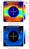 |
Fig. 8. Top panel: Solar wind speed map derived from Metis observations on January 14, 2021, with the following coronal model assumptions: Te is the radial profile from Gibson et al. (1999), Tk = 1.0 MK, Ki = 1, and AHe = 10%. Bottom panel: Solar wind speed uncertainty maps computed from the estimated errors on pB and H I Lyα intensity measurements. |
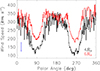 |
Fig. 9. Solar wind speed latitudinal profiles at 4.0 and 6.0 R⊙ from the map in the top panel of Fig. 8. The blue error bar in the left corner represents the variability of the computed wind speed values from the uncertainties on the measured H I Lyα intensity and pB. |
An estimate of the uncertainty in the determination of the solar wind speed that is due to the measurement errors was obtained by calculating the dispersion of the results, defined as the difference for each pixel between the minimum and maximum speed values derived by varying the pB and H I Lyα intensity values by ±10% and ±20%, respectively. These variations were chosen based on the average errors reported for the two channels in Sect. 3. A map of the solar wind speed uncertainty calculated in this way is shown in the bottom panel of Fig. 8. The analysis yields an average uncertainty of approximately ±25 km s−1, as shown by the blue error bar in Fig. 9. The uncertainty is about ±15 km s−1 in fast wind regions and increases to ±40 km s−1 in equatorial regions, where the wind speed is generally lower. The zero values in the speed image as well as in the uncertainty image, indicated by the black points, represent the positions where the diagnostic was unable to determine the solar wind speed because the signal-to-noise ratio was too low, for instance, in the NW sector at heights greater than 5 R⊙.
The typical bimodal behavior of the solar wind outflow velocities characterizing the near-minimum phases of solar activity is generally evident: The velocities in the regions around the poles are significantly higher than in those around the solar equator. They range from about 250 to more than 300 km s−1 for the former, and from lower than 130 to about 180 km s−1 for the latter. The transition between the equatorial streamer belt and the surrounding regions is quite sharp, and the wind speed increases steeply at higher latitudes. The outflow velocities obtained in the equatorial regions are consistent with those determined by Antonucci et al. (2023) in the slow wind belt that runs along the coronal current sheet. The polar regions show a remarkable scatter in the latitudinal profiles of the wind speed that is caused by the higher level of noise that affects the Lyα line intensities. On the other hand, we expect to detect a low coronal signal, in particular, around 6 R⊙, because the Doppler dimming of the Lyα line at velocities higher than 300 km s−1 is significant. This is close to the limit for which the Doppler dimming diagnostics can be applied (see the bottom panel in Fig. 1). Consequently, the observed line intensities at these heights are probably mainly due to the interplanetary H I Lyα emission (see Fig. 4, bottom panel), so that the resulting outflow velocity values cannot be taken as representative of the dynamic conditions in the polar corona regions.
5. Dependence of the wind speed value on the assumed coronal parameters
It is important to investigate the dependence of the derived outflow velocities on the values of the physical quantities that are representative of the coronal environment we adopted in the synthesis of the resonantly scattered H I Lyα line intensity. Therefore, we present and compare some of the results that were obtained with different assumed coronal parameters, such as
-
Te, considering at all latitudes the radial profiles determined by Gibson et al. (1999) and Vásquez et al. (2003), together with some constant values throughout the examined corona;
-
Tk, considering a set of values ranging from 1.0 to 3.0 MK, that were each time assumed to be constant throughout the examined corona;
-
isotropic or anisotropic Tk distribution, with the anisotropy factor Ki in the range from 1 to 2;
-
He abundance, equal to 2.5% and 10%.
Figures 10 and 11 clearly show that an increase in the adopted values for the electron temperatures results in a decrease in the determined outflow velocities. Owing to the reduction in the neutral hydrogen ion fraction at higher temperatures, a lower speed value is required to match the reduction in the Lyα line intensities with respect to the static corona case. For example, in equatorial and mid-latitude regions at 5 R⊙, an increase in electron temperature by a factor of two corresponds to a decrease in the outflow velocity by about a factor of two (see Fig. 11).
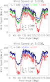 |
Fig. 10. Computed solar wind speed as a function of latitude at 5 R⊙ with a different assumption on the electron temperature. The black line in the top panel corresponds to the assumption of a temperature profile from Gibson et al. (1999) (G99), The green, blue, and red lines show Te = 0.4 MK, Te = 0.6 MK, and Te = 1.0 MK, respectively. In the bottom panel, overlapping the speeds obtained with Gibson et al. (1999) (G99), we show the speeds with the temperature profiles given by Vásquez et al. (2003). The blue line shows a coronal hole profile (V03CH), and the red line shows a streamer profile (V03ST). |
The electron temperature cannot be varied arbitrarily, but is upper range is limited by the hydrogen kinetic temperature adopted for the calculation (see also Sect. 4.2). The solid curves in Fig. 11 that are relevant to the assumption Tk = 1 MK therefore cannot extend beyond 1 MK. For higher hydrogen kinetic temperatures (e.g., Tk = 2 MK; dashed lines in Fig. 11), however, it is evident that according to the Lyα line intensities observed at equatorial and mid-latitudes at 5 R⊙, the electron temperature cannot exceed values around 1.2−1.4 MK for reasonable values of the outflow velocities. This limit is set by the reduction of the neutral hydrogen density due to ionization, so that the synthetic Lyα intensity for a static corona is already lower than the measured value above a certain temperature threshold. Therefore, the application of the Doppler dimming technique can also provide a constraint (an upper limit, in this case) on the electron temperature.
For the dependence on the adopted neutral hydrogen kinetic temperature, the outflow velocity increases as the kinetic temperature increases. As shown in Fig. 12, at 5 R⊙ we note a velocity increase by about 100 km s−1 (∼30%) in the polar regions, when the kinetic temperature increases from 1.0 to 3.0 MK. A smaller increase (15−20 km s−1) occurs in the equatorial regions for the same variations of kinetic temperature. Higher neutral hydrogen kinetic temperatures imply broader coronal Lyα absorption profiles, so that higher velocities (corresponding to higher Doppler shifts) are required to reduce the scattering efficiency. This results in the same intensity reduction of the scattered radiation. We note that Dolei et al. (2015, 2018) described the opposite behavior for outflow velocities below 100 km s−1. Due to the particular shape of the exciting chromospheric Lyα line profile (see Fig. 1), higher kinetic temperatures result in lower velocities.
The results discussed above agree in general with the work reported by Dolei et al. (2015, 2018), who investigated, in particular, the dependence of the derived outflow velocities on the values of the coronal electron temperature and the H I kinetic temperature using coronal Lyα intensity maps reconstructed from daily UVCS/SOHO spectroscopic observations.
The isotropic or anisotropic character of the kinetic temperature distribution of the coronal scattering atoms also affects the wind speed determination. An anisotropy factor Ki > 1 implies a lower value of T|| with respect to the isotropic condition, that is, a narrower coronal Lyα absorption profile. Based on the above discussion of the effect of the adopted neutral hydrogen kinetic temperature, this results in lower values for the determined outflow velocities, as shown in Fig. 13 for the wind speeds obtained at 5 R⊙. In this case, T|| = Te = T⊥/2 gives speed reductions of about 40 km s−1 and about 10 km s−1 in the polar and equatorial regions, respectively. Romoli et al. (2021) and Antonucci et al. (2023) also recently showed a similar behavior in their analysis of the first observations performed by Metis.
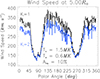 |
Fig. 13. Computed solar wind speed as a function of latitude at 5 R⊙ with two different assumption on the kinetic temperature distribution. Black shows the isotropic distribution Ki = 1, and blue shows the anisotropic distribution Ki = 2. |
The effect on the determination of the outflow velocity of the adopted He abundance is more limited. A changed abundance from 10% to 2.5% reduces the wind speed at 5 R⊙ by about 5% for velocities of about 100 km s−1 and by a smaller percentage for higher velocities.
On the basis of the above evaluations, we remark that the variations in the wind speed values induced by the assumption of different values of electron and neutral hydrogen kinetic temperatures in the Doppler dimming analysis can be significantly larger than the uncertainties in the determination of the solar wind speed because of the measurement errors in the pB and and H I Lyα intensity. The variations in the adopted anisotropy factor and He abundance induce wind speed variations that are comparable with the uncertainties from the measurement errors.
Not all the electron and kinetic temperatures we explored are physically viable. By relying on theoretical or experimental justifications, the uncertainties associated with the parameterization of the coronal model can be reduced. It remains essential in this type of diagnostics to ensure that the observed speed variations across different coronal structures are not predominantly influenced by the assumptions on the physical parameters required in the calculations, however.
6. Results and discussions
The solar wind speed map we showed at the end of Sect. 4 (see Fig. 8, top panel), obtained from H I Lyα and visible-light pB Metis observations on January 14, 2021, can be considered as the reference map in this work. In addition, we calculated the wind outflow velocity maps from the Metis observations obtained on June 21, 2020 (see Fig. 14), soon after the first perihelion of the Solar Orbiter mission, and on February 12 and 17, 2021 (see Figs. 15 and 16, respectively), after the second perihelion. These maps were calculated assuming the same coronal model parameters as for January 14, 2021, and they appear to be very similar to the map that is relevant to that day, in particular, to the global structure of the wind speed in the outer solar corona observed by Metis. It exhibits the typical configuration of the corona near solar minimum and is characterized by a quasi-dipolar magnetic field topology, with a bright equatorial streamer belt that embeds the coronal/heliospheric current sheet, where the outflow velocities are generally lower. This separates the two large open-field regions located above the solar poles, from which the fast solar wind comes. The transition between the slow and fast wind is quite sharp, with a steep increase in the wind speed. This characteristic aspect has also been pointed out and discussed by Antonucci et al. (2023).
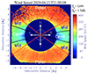 |
Fig. 14. Solar wind speed map derived from Metis observations on June 21, 2020, with the coronal model assumptions of the Te radial profile from Gibson et al. (1999), Tk = 1.0 MK, Ki = 1, and AHe = 10%. The lines overlaid on the image identify the angular sectors we defined to study the radial speed trends for different coronal structures. The regions between the red lines are associated with polar coronal holes, and those between the black lines correspond to equatorial regions. |
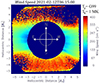 |
Fig. 15. Solar wind speed map derived from Metis observations on February 12, 2021, with the coronal model assumptions of the Te radial profile from Gibson et al. (1999), Tk = 1.0 MK, Ki = 1, and AHe = 10%. |
 |
Fig. 16. Solar wind speed map derived from Metis observations on February 17, 2021, with the coronal model assumptions of the Te radial profile from Gibson et al. (1999), Tk = 1.0 MK, Ki = 1, and AHe = 10%. |
On the other hand, we noted some differences in the velocity map obtained in June 2020, closer to the phase of solar activity minimum, and the maps obtained in January and February 2021, when the level of solar activity was already slightly higher. In particular, the sharp transition between lower and higher wind speeds exhibits a shift toward higher latitudes in the north and south regions from June 2020 to January–February 2021, as a result of the warping of the equatorial streamer belt. This follows from the higher inclination of the heliospheric current sheet with respect to the equatorial plane with the increased solar magnetic activity (see, e.g., Antonucci et al. 2020a).
The observational period from January 14 to January 17, 2021, was covered at a regular 4-hour cadence, with only three data gaps. This enables us to study the evolution of the solar corona in terms of visible and ultraviolet emission, as well as solar wind speed, by reconstructing the synoptic maps at fixed heliocentric distances. A concise visualization of the variation in these parameters is thus possible (see, e.g., Lamy et al. 2020). In Fig. 17 we present the synoptic maps at 4 R⊙.
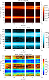 |
Fig. 17. Synoptic maps at 4 R⊙ of pB (top panel), H I Lyα intensity (middle panel), and derived solar wind speed (bottom panel) from Metis observations from January 14 to 17, 2021. The solar wind speed was computed with the following coronal model assumptions: Te is the radial profile from Gibson et al. (1999), Tk = 1.0 MK, Ki = 1, and AHe = 10%. The polar angle is measured counterclockwise from the north pole, so that PA = 90° and 270° indicate the equatorial regions. |
In the VL and UV channels (see the top and middle panels in Fig. 17), the coronal emission mainly remains concentrated in the equatorial streamer belt, where the coronal/heliospheric current sheet that separates the two regions of opposite magnetic polarity that are located above the poles (dipolar configuration) is likely to form, as expected during near-minimum levels of solar activity. While the streamer above the east limb exhibited the characteristic cusp shape typical of equatorial streamers at solar minimum throughout the examined temporal interval, the streamer above the west limb appears to be more diffuse and exhibits several thin brighter features that are clearly evident in the visible light between ∼40°S and 30°N. This makes it more difficult to firmly identify the position of the heliospheric current sheet, as already remarked in the description of Fig. 3. We also note that during the last days of the examined temporal interval, the equatorial region at the west limb appears to be slightly broader and shows the evolution of the streamer belt over some days.
In both cases, however, the transition between the equatorial streamer belt and the surrounding regions is quite sharp, with a steep drop in coronal emission at higher latitudes in the two Metis passbands (by at least a factor of 5 in the pB and by a factor of 4 in the H I Lyα).
The typical bimodal behavior of the synoptic maps of the coronal visible and ultraviolet emission is reflected in the synoptic map of the solar wind outflow velocity (see the bottom panel in Fig. 17), which exhibits the characteristics of the near-minimum phases of solar activity: The velocities in the regions around the poles are significantly higher than those around the solar equator. The transition between the lower equatorial velocities and the surrounding higher velocity regions is quite sharp, with a steep increase in the wind speed over a latitude range of only 10−20°. This characteristic behavior holds throughout the solar longitude range that was covered during the days of the Metis observations. Moreover, the equatorial region at the west limb with its lower wind speed appears to be slightly broader during the last days of the examined temporal interval. This reflects the evolution of the streamer belt reported above. The comparison of synoptic maps at different heights can be used to examine the characteristics of the behaviors discussed above at different heliocentric distances.
The bimodal profile of the solar wind near solar minimum is clearly visible in the bottom panel of Fig. 17 at a fixed height. It is also evident in the radial speed profiles, averaged over various angular regions that we show in Fig. 18. In this case, an angular sector of ±10° around the interface regions at mid-latitudes was selected, while for the polar and equatorial sectors, the angular regions we considered were those bounded by the edges defined at mid-latitudes (see Fig. 14). We also note that the radial profiles of the wind speed are clearly higher in the two polar regions, although they exhibit a lower gradient there, implying a lower acceleration. This is evidence that the energy dissipation is more concentrated at lower heights in these regions than in the others. In addition, the radial profiles of the polar speed shown in Fig. 18 agree well within the estimated uncertainties with the average radial profile of the neutral hydrogen outflow velocity determined at polar latitudes by Telloni et al. (2023). The velocity maps presented here are complementary to the map obtained from UVCS spectroscopic observations during the solar minimum at the end of solar cycle 22 (see Fig. 4 in Giordano et al. 1997). Observations of the doublet emitted by O5+ ions in the region between 1.4 and 3.8 R⊙ highlighted the bimodal structure of the solar wind by identifying coronal regions with velocities below or above 100 km s−1. Giordano et al. (1997) showed that the velocity in the equatorial region tends to remain below 100 km s−1 up to a distance of approximately 3.5 R⊙. This agrees within uncertainties with the results presented in Fig. 18.
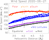 |
Fig. 18. Average radial profiles of the solar wind speed for different latitudinal sectors from the observations made on June 21, 2020. The blue dots show the values for the ±10° region around the interface zones between streamers and coronal holes associated with intermediate latitudes. The black and purple dots correspond to the equatorial regions located between the two interface zones, and the red and orange dots show the polar regions. A sample of the estimated error bars, determined at 4 R⊙ on the base of instrumental uncertainties, is shown. |
We reported the analysis of simultaneous UV H I Lyα and visible-light polarized-brightness images of the solar corona obtained by the Metis coronagraph on board the Solar Orbiter mission. It enabled us to create global maps of the hydrogen outflow velocity in the inner heliosphere. This provided an unprecedented view of the solar wind acceleration region over a wide range of heliocentric distances, from 1.7 to 9 R⊙, depending on the spacecraft distance from the Sun.
Maps like this can be obtained daily and might be used to investigate the detailed structure of the solar wind and its evolution during the time that is covered by the observations of Metis. This approach can be more efficient when the spacecraft is closer to the Sun (minimum perihelion at 0.28 au) because the Metis field of view images brighter coronal regions and the detected signal is higher and less noisy, which results in lower uncertainties in the wind speeds determined by the Doppler dimming technique. We plan to extend our investigation in this sense in future works.
The latitudinal and radial properties of the solar wind extracted from the calculated maps, including the velocity gradients that helped us to locate the regions of energy input and acceleration of the wind, provide much physical information that can be interpreted after a comparison with the configuration and strength of the coronal magnetic fields as derived from MHD models and accurate extrapolations of the photospheric fields.
On the other hand, this wealth of physical information offers the possibility of placing accurate constraints on the development of theoretical models of coronal structures and source regions of the solar wind.
Laboratory for Atmospheric and Space Physics (2005). LASP Interactive Solar Irradiance Datacenter. Laboratory for Atmospheric and Space Physics. https://doi.org/10.25980/L27Z-XD34
Acknowledgments
Solar Orbiter is a space mission of international collaboration between ESA and NASA, operated by ESA. Metis was built and operated with funding from the Italian Space Agency (ASI), under contracts to the National Institute of Astrophysics (INAF) and industrial partners. Metis was built with hardware contributions from Germany (Bundesministerium für Wirtschaft und Energie through DLR), from the Czech Republic (PRODEX) and from ESA. This study was carried out in part within the Space It Up project funded by the Italian Space Agency, ASI, and the Ministry of University and Research, MUR, under contract n. 2024-5-E.0 – CUP n. I53D24000060005. The authors thank the former PI, Ester Antonucci, for leading the development of Metis until the final delivery to ESA, as well as for her constructive comments to a first draft of the manuscript. They also thank Dr. S. Dolei and G. Capuano for their contribution to the early development of the code.
References
- Abbo, L., Ofman, L., Antiochos, S. K., et al. 2016, Space Sci. Rev., 201, 55 [NASA ADS] [CrossRef] [Google Scholar]
- Akinari, N. 2007, ApJ, 660, 1660 [Google Scholar]
- Allen, L. A., Habbal, S. R., & Hu, Y. Q. 1998, J. Geophys. Res., 103, 6551 [NASA ADS] [CrossRef] [Google Scholar]
- Andretta, V., Bemporad, A., De Leo, Y., et al. 2021, A&A, 656, L14 [NASA ADS] [CrossRef] [EDP Sciences] [Google Scholar]
- Antonucci, E., Dodero, M. A., & Giordano, S. 2000, Sol. Phys., 197, 115 [NASA ADS] [CrossRef] [Google Scholar]
- Antonucci, E., Abbo, L., & Telloni, D. 2012, Space Sci. Rev., 172, 5 [NASA ADS] [CrossRef] [Google Scholar]
- Antonucci, E., Harra, L., Susino, R., & Telloni, D. 2020a, Space Sci. Rev., 216, 117 [CrossRef] [Google Scholar]
- Antonucci, E., Romoli, M., Andretta, V., et al. 2020b, A&A, 642, A10 [NASA ADS] [CrossRef] [EDP Sciences] [Google Scholar]
- Antonucci, E., Downs, C., Capuano, G. E., et al. 2023, Phys. Plasmas, 30, 022905 [Google Scholar]
- Auchère, F. 2005, ApJ, 622, 737 [Google Scholar]
- Beckers, J. M., & Chipman, E. 1974, Sol. Phys., 34, 151 [Google Scholar]
- Bessell, M. S., Castelli, F., & Plez, B. 1998, A&A, 333, 231 [NASA ADS] [Google Scholar]
- Brueckner, G. E., Howard, R. A., Koomen, M. J., et al. 1995, Sol. Phys., 162, 357 [NASA ADS] [CrossRef] [Google Scholar]
- Capuano, G. E., Dolei, S., Spadaro, D., et al. 2021, A&A, 652, A85 [NASA ADS] [CrossRef] [EDP Sciences] [Google Scholar]
- Cranmer, S. R. 2020, ApJ, 900, 105 [Google Scholar]
- Cranmer, S. R., Kohl, J. L., Noci, G., et al. 1999, ApJ, 511, 481 [CrossRef] [Google Scholar]
- Cranmer, S. R., Gibson, S. E., & Riley, P. 2017, Space Sci. Rev., 212, 1345 [Google Scholar]
- De Leo, Y., Burtovoi, A., Teriaca, L., et al. 2023, A&A, 676, A45 [NASA ADS] [CrossRef] [EDP Sciences] [Google Scholar]
- De Leo, Y., Burtovoi, A., Teriaca, L., et al. 2025, A&A, 697, A73 [NASA ADS] [CrossRef] [EDP Sciences] [Google Scholar]
- Dere, K. P., Landi, E., Mason, H. E., Monsignori Fossi, B. C., & Young, P. R. 1997, A&AS, 125, 149 [NASA ADS] [CrossRef] [EDP Sciences] [Google Scholar]
- Dodero, M. A., Antonucci, E., Giordano, S., & Martin, R. 1998, Sol. Phys., 183, 77 [Google Scholar]
- Dolei, S., Spadaro, D., & Ventura, R. 2015, A&A, 577, A34 [NASA ADS] [CrossRef] [EDP Sciences] [Google Scholar]
- Dolei, S., Spadaro, D., & Ventura, R. 2016, A&A, 592, A137 [NASA ADS] [CrossRef] [EDP Sciences] [Google Scholar]
- Dolei, S., Susino, R., Sasso, C., et al. 2018, A&A, 612, A84 [NASA ADS] [CrossRef] [EDP Sciences] [Google Scholar]
- Dolei, S., Spadaro, D., Ventura, R., et al. 2019, A&A, 627, A18 [NASA ADS] [CrossRef] [EDP Sciences] [Google Scholar]
- Domingo, V., Fleck, B., & Poland, A. I. 1995, Sol. Phys., 162, 1 [Google Scholar]
- Fineschi, S., Korendyke, C. M., Siegmund, O. H., & Woodgate, B. E. 2000, SPIE Conf. Ser., 4139 [Google Scholar]
- Fineschi, S., Antonucci, E., Romoli, M., et al. 2003, SPIE Conf. Ser., 4853, 162 [Google Scholar]
- Fineschi, S., Naletto, G., Romoli, M., et al. 2020, Exp. Astron., 49, 239 [Google Scholar]
- Foukal, P. 1990, Solar Astrophysics (New York: Wiley) [Google Scholar]
- Fox, N. J., Velli, M. C., Bale, S. D., et al. 2016, Space Sci. Rev., 204, 7 [Google Scholar]
- Gabriel, A. H. 1971, Sol. Phys., 21, 392 [Google Scholar]
- Gibson, S. E., Fludra, A., Bagenal, F., et al. 1999, J. Geophys. Res., 104, 9691 [Google Scholar]
- Giordano, S., Antonucci, E., Benna, C., et al. 1997, ESA Spec. Publ., 415, 327 [Google Scholar]
- Giordano, S., Antonucci, E., Noci, G., Romoli, M., & Kohl, J. L. 2000, ApJ, 531, L79 [Google Scholar]
- Hundhausen, A. J. 1972, Coronal Expansion and Solar Wind (New York: Springer-Verlag) [Google Scholar]
- Hyder, C. L., & Lites, B. W. 1970, Sol. Phys., 14, 147 [Google Scholar]
- Kohl, J. L., & Withbroe, G. L. 1982, ApJ, 256, 263 [Google Scholar]
- Kohl, J. L., Esser, R., Gardner, L. D., et al. 1995, Sol. Phys., 162, 313 [Google Scholar]
- Kohl, J. H., Noci, G., Antonucci, E., et al. 1997, Adv. Space Res., 20, 3 [Google Scholar]
- Kohl, J. L., Noci, G., Antonucci, E., et al. 1998, ApJ, 501, L127 [Google Scholar]
- Kohl, J. L., Noci, G., Cranmer, S. R., & Raymond, J. C. 2006, A&ARv, 13, 31 [Google Scholar]
- Lamy, P., Llebaria, A., Boclet, B., et al. 2020, Sol. Phys., 295, 89 [CrossRef] [Google Scholar]
- Landi, E., Young, P. R., Dere, K. P., Del Zanna, G., & Mason, H. E. 2013, ApJ, 763, 86 [CrossRef] [Google Scholar]
- Leblanc, Y., Dulk, G. A., & Bougeret, J.-L. 1998, Sol. Phys., 183, 165 [NASA ADS] [CrossRef] [Google Scholar]
- Liberatore, A., Fineschi, S., Casti, M., et al. 2023, A&A, 672, A14 [NASA ADS] [CrossRef] [EDP Sciences] [Google Scholar]
- Lionello, R., Linker, J. A., & Mikić, Z. 2009, ApJ, 690, 902 [CrossRef] [Google Scholar]
- Machol, J., Snow, M., Woodraska, D., et al. 2019, Earth Space Sci., 6, 2263 [Google Scholar]
- Mikić, Z., Downs, C., Linker, J. A., et al. 2018, Nat. Astron., 2, 913 [Google Scholar]
- Moses, J. D., Antonucci, E., Newmark, J., et al. 2020, Nat. Astron., 4, 1134 [Google Scholar]
- Müller, D., St. Cyr, O. C., Zouganelis, I., et al. 2020, A&A, 642, A1 [Google Scholar]
- Noci, G., Kohl, J. L., & Withbroe, G. L. 1987, ApJ, 315, 706 [Google Scholar]
- Noci, G., Kohl, J. L., Antonucci, E., et al. 1997, ESA Spec. Publ., 404, 75 [Google Scholar]
- Olsen, E. L., Leer, E., & Holzer, T. E. 1994, ApJ, 420, 913 [NASA ADS] [CrossRef] [Google Scholar]
- Raymond, J. C., Kohl, J. L., Noci, G., et al. 1997, Sol. Phys., 175, 645 [Google Scholar]
- Romoli, M., Antonucci, E., Andretta, V., et al. 2021, A&A, 656, A32 [NASA ADS] [CrossRef] [EDP Sciences] [Google Scholar]
- Russano, G., Andretta, V., De Leo, Y., et al. 2024, A&A, 683, A191 [NASA ADS] [CrossRef] [EDP Sciences] [Google Scholar]
- Rybicki, G. B., & Lightman, A. P. 1979, Radiative Processes in Astrophysics (New York: Wiley) [Google Scholar]
- Spadaro, D., Susino, R., Ventura, R., Vourlidas, A., & Landi, E. 2007, A&A, 475, 707 [NASA ADS] [CrossRef] [EDP Sciences] [Google Scholar]
- Strachan, L., Suleiman, R., Panasyuk, A. V., Biesecker, D. A., & Kohl, J. L. 2002, ApJ, 571, 1008 [Google Scholar]
- Susino, R., Ventura, R., Spadaro, D., Vourlidas, A., & Landi, E. 2008, A&A, 488, 303 [NASA ADS] [CrossRef] [EDP Sciences] [Google Scholar]
- Telloni, D., Andretta, V., Antonucci, E., et al. 2021, ApJ, 920, L14 [NASA ADS] [CrossRef] [Google Scholar]
- Telloni, D., Antonucci, E., Adhikari, L., et al. 2023, A&A, 670, L18 [NASA ADS] [CrossRef] [EDP Sciences] [Google Scholar]
- Uslenghi, M., Andretta, V., Teriaca, L., et al. 2024, SPIE Conf. Ser., 13103, 1310324 [Google Scholar]
- van de Hulst, H. C. 1950, Bull. Astron. Inst. Netherlands, 11, 135 [Google Scholar]
- Vásquez, A. M., van Ballegooijen, A. A., & Raymond, J. C. 2003, ApJ, 598, 1361 [Google Scholar]
- Vásquez, A. M., Nuevo, F. A., Burtovoi, A., et al. 2025, Sol. Phys., 300, 4 [Google Scholar]
- Withbroe, G. L., Kohl, J. L., Weiser, H., & Munro, R. H. 1982, Space Sci. Rev., 33, 17 [Google Scholar]
- Zirker, J. B. 1977, Rev. Geophys. Space Phys., 15, 257 [CrossRef] [Google Scholar]
Appendix
In a spherical coordinate system with origin in the point of scattering and polar axis corresponding to the line connecting that point to Sun’s center, the H I Lyα line intensity (in units of photons cm−2s−1sr−1) emitted towards an observer in the n direction, Ir(n), given by the Eq. 1, can be rewritten as
 (A.1)
(A.1)
where B12 = 8.48995 × 10⁹ (sr cm2 erg−1 s−1) is the Einstein coefficient for the absorption related to Lyα transition (Rybicki & Lightman 1979; Foukal 1990), h is the Planck constant (ergs), λ0 is the rest wavelength of the H I Lyα line (cm), and c is the speed of light (cm s−1).
The numerical density of neutral hydrogen, nHI (cm−3) in Eq. 1, considering that  , can be rewritten as
 (A.2)
(A.2)
where the coefficient
 (A.3)
(A.3)
is determined for a fully ionized plasma with a given helium abundance AHe (i.e., npe values are 0.833 or 0.952 for 10% or 2.5% in the number helium abundance, respectively), RHI is the neutral hydrogen ionization fraction (depending on the coronal electron temperature Te) given by the equilibrium tables from CHIANTI database (see, e.g., Dere et al. 1997; Landi et al. 2013), ne is the electron density. The term  represents the integration of the emissivity along the line of sight defined by the x-axis (see Fig. 2). The geometric scattering function (Beckers & Chipman 1974)
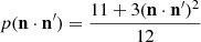
represents the probability that a chromospheric photon, coming from the direction n′, can be scattered in the direction n, that is through the angle ψ, so that n ⋅ n′ = cosψ.
The integral over the solid angle subtended by the chromosphere at the point of the scattering, ∫Ω…dΩ, in the Eq. 1, can be written as ∫θ∫ϕ…sin θ dθ dϕ, where θ is the angle between the wind speed direction, vout, which is assumed as radial, and the direction of the incoming radiation, n′. The angle θ spans from zero, when the radiation comes from the Sun center to a maximum value, α2, when it comes from the limb,  , where ρ is the distance of the scattering point from Sun center,
 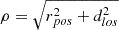 where rpos and dlos are the distances in the plane of the sky and from that plane, respectively. The polar angle ϕ covers the entire disk, so it ranges from 0 to 2π.
For the incoming chromospheric Lyα radiation, Iex(λ − λ0, n′) we use the analytical profile proposed by Auchère (2005) which approximate the observed profile with a combination of three gaussians profiles:
![Mathematical equation: $$ \begin{aligned} \Psi (\lambda \prime -\lambda _0) = \sum _{i = 1}^n\frac{a_i}{{\sigma _i}\sqrt{\pi }}\exp {\Biggl [{-\frac{(\lambda \prime -\lambda _0- \delta \lambda _i)^2}{\sigma _i^2}}\Biggr ]} \end{aligned} $$](/articles/aa/full_html/2025/09/aa54105-25/aa54105-25-eq13.gif) (A.4)
(A.4)
where the values of the parameters, ai, σi and λi, updated by Auchère (2024, private communication), are given in the Table A.1.
Gaussian fitting parameters of the normalized Lyα chromospheric profile (Auchère 2005)
Therefore, the incident profile is computed as
 (A.5)
(A.5)
where Ichr (photons cm−2s−1sr−1) is the total chromospheric intensity reported in Table 2.
The function f(v) is the velocity distribution function of the coronal hydrogen atoms, and the Dirac delta function takes into account that the chromospheric photons incident on P from different directions n′ within the solid angle that can be scattered by coronal atoms with velocity v are those with 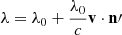 .
.
The random motion velocity of coronal atoms, f(v), can be assumed bi-Maxwellian, considering different velocities in the direction parallel to the radial (along which the solar wind flows) and the two perpendicular directions. Moreover, decomposing the parallel velocity of the atoms into the sum of their random motion velocity and the bulk outflow velocity, vout, we can write
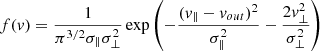 (A.6)
(A.6)
where: v∥ is the velocity component in the direction parallel to the radial, v⊥ is the velocity component in the perpendicular directions.  , and
, and  are the widths of the velocity distribution in the parallel and perpendicular directions, respectively. KB is the Boltzmann constant (erg K−1), T∥ and T⊥ are the temperatures (K) of the ions in the parallel and perpendicular to radial directions, mp is the proton mass (g).
To compute the effective absorption profile we rotate the reference frame to have one axis coincident with the direction, n′, of the incident chromospheric photons


where θ is the angle between vout and n′. Integrating f(v) over the plane perpendicular to n′ we calculate the effective absorption profile for all incident radiation directions from the solar disk as
 (A.7)
(A.7)
where σe is the width of the effective velocity distribution, which corresponds to the width of the effective absorption profile, given by
 (A.8)
(A.8)
where Tk, the kinetic temperature, is equal to T⊥, and Ki is the anisotropy coefficient defined as
 (A.9)
(A.9)
The analytical chromospheric exciting profile (Eq. A.4, and A.5), and the coronal absorption profiles (Eq. A.7 and A.8) allow the analytical integration to be performed over the kinetic velocity and wavelength of Eq. A.1 to obtain
![Mathematical equation: $$ \begin{aligned}&I_{r}\left(\mathbf n \right) = \frac{1}{\sum _{i = 1}^{n}a_i} B_{12} \frac{h\lambda _0}{4\pi }\,n_{pe}\,I_{disk} \,\int _{-\infty }^{+\infty }{n_eR_{H_i}dx}\nonumber \\&\qquad \int _{0}^{\alpha _2}\left[\frac{1}{12}\left(11+3 \left(\cos ^2{\phi }\cos ^2{\theta }+\frac{1}{2} \sin ^2{\phi }\sin ^2{\theta }\right)\right)\right]\nonumber \\&\qquad \quad \frac{1}{2\sqrt{\pi }}\sum _{i = 1}^{n}{\frac{a_i}{\sqrt{w^2+\sigma _i^2}} \exp \left[-\frac{\left(\delta \lambda _i-\frac{\lambda _0}{c}v_{out}\cos {\theta }\right)^2}{w^2+\sigma _i^2}\right]\sin \theta \ d\theta } \end{aligned} $$](/articles/aa/full_html/2025/09/aa54105-25/aa54105-25-eq24.gif) (A.10)
(A.10)
where α2 is the maximum value of θ that depends on the distance of the scattering point from the incident radiation source.
The previous equation is numerically integrated considering the length of the LOS equal ranging from −2rmax to +2rmax, where rmax is the maximum observed heliocentric distance, and the length of the elements along the LOS, dx = 0.5R⊙. It has been verified that a finer sampling increases the computation time without significantly changing the results obtained. Regarding integration on the solid angle, in the analytical formulation of Eq. A.10, it reduces to the integration over the angle θ, which varies from 0 to 2α2, with a chosen step size  .
.
All Tables
Gaussian fitting parameters of the normalized Lyα chromospheric profile (Auchère 2005)
All Figures
|
Fig. 1. Top panel: Chromospheric Lyα profile (red) and coronal absorption Lyα profile (blue) for a static corona (vout = 0 km s−1). Middle panel: Chromospheric and absorption profiles Doppler shifted for an outflow velocity of 150 km s−1. The absorption coronal profile is calculated as a Gaussian shape for a neutral hydrogen kinetic temperature equal to 1.5 MK. Bottom panel: I(vout)/I(vout = 0) calculated for three different neutral hydrogen kinetic temperatures, Tk = 0.8 MK (black), Tk = 1.5 MK (blue), and Tk = 3.0 MK (red). |
| In the text | |
|
Fig. 2. Simplified geometry of the radiation from the chromospheric point S, resonantly scattered in the coronal point P at the heliocentric distance r. The x-axis represents the line of sight of the observer, vout is the outflow velocity, which we assumed to be radial, and Ω is the solid angle subtended by the point P. The vectors n′ and n give the directions of the incident and scattered photons, respectively. |
| In the text | |
|
Fig. 3. Simultaneous maps of visible-light pB (top panel) and H I Lyα intensity (bottom panel) from the Metis observations performed on January 14, 2021, at 00:45 UT. The solar disk was detected in both images at 00:45 UT by the EUI instrument on board the Solar Orbiter at a wavelength of 171 A (gray scale) and was superimposed in the center. |
| In the text | |
|
Fig. 4. Latitudinal distributions of the visible-light pB (top panel) and H I Lyα intensity (bottom panel) at 4.0 and 6.0 R⊙, derived from the maps shown in Fig. 3. The latitude is expressed in terms of the polar angle, measured counterclockwise from the north pole. In the bottom panel, the horizontal dashed blue lines mark the expected range of the H I Lyα interplanetary emission (3 − 6 × 10⁷ photons s−1 cm−2 sr−1; see, e.g., Kohl et al. 1997; Akinari 2007). |
| In the text | |
|
Fig. 5. Electron density map from Metis pB observations performed on January 14, 2021, at 00:45 UT. |
| In the text | |
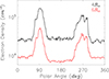 |
Fig. 6. Electron density latitudinal profiles at 4.0 and 6.0 R⊙ from the map in Fig. 5. |
| In the text | |
|
Fig. 11. Computed solar wind speed as a function of electron temperature at 5 R⊙ for different latitudes (polar: black, mid: red, and equatorial: blue) and with two different assumptions on the kinetic temperature: Tk = 1.0 MK (full line and circles) and Tk = 2.0 MK (dashed line and open circles). |
| In the text | |
|
Fig. 12. Computed solar wind speed as a function of latitude at 5 R⊙, adopting the electron temperature profile from Gibson et al. (1999) and with five different assumptions on the kinetic temperature. |
| In the text | |
|
Fig. 7. Electron temperature radial profile from Gibson et al. (1999) (black), Vásquez et al. (2003), coronal hole (blue), and streamer (red). The vertical dashed lines show the range of the field of view observed by Metis on January 14, 2021, and the horizontal dashed lines represents the different constant values: 0.4 (blue), 0.6 (green), and 1.0 (red) MK) assumed to compute the wind speed presented in Fig. 10. |
| In the text | |
|
Fig. 8. Top panel: Solar wind speed map derived from Metis observations on January 14, 2021, with the following coronal model assumptions: Te is the radial profile from Gibson et al. (1999), Tk = 1.0 MK, Ki = 1, and AHe = 10%. Bottom panel: Solar wind speed uncertainty maps computed from the estimated errors on pB and H I Lyα intensity measurements. |
| In the text | |
|
Fig. 9. Solar wind speed latitudinal profiles at 4.0 and 6.0 R⊙ from the map in the top panel of Fig. 8. The blue error bar in the left corner represents the variability of the computed wind speed values from the uncertainties on the measured H I Lyα intensity and pB. |
| In the text | |
|
Fig. 10. Computed solar wind speed as a function of latitude at 5 R⊙ with a different assumption on the electron temperature. The black line in the top panel corresponds to the assumption of a temperature profile from Gibson et al. (1999) (G99), The green, blue, and red lines show Te = 0.4 MK, Te = 0.6 MK, and Te = 1.0 MK, respectively. In the bottom panel, overlapping the speeds obtained with Gibson et al. (1999) (G99), we show the speeds with the temperature profiles given by Vásquez et al. (2003). The blue line shows a coronal hole profile (V03CH), and the red line shows a streamer profile (V03ST). |
| In the text | |
|
Fig. 13. Computed solar wind speed as a function of latitude at 5 R⊙ with two different assumption on the kinetic temperature distribution. Black shows the isotropic distribution Ki = 1, and blue shows the anisotropic distribution Ki = 2. |
| In the text | |
|
Fig. 14. Solar wind speed map derived from Metis observations on June 21, 2020, with the coronal model assumptions of the Te radial profile from Gibson et al. (1999), Tk = 1.0 MK, Ki = 1, and AHe = 10%. The lines overlaid on the image identify the angular sectors we defined to study the radial speed trends for different coronal structures. The regions between the red lines are associated with polar coronal holes, and those between the black lines correspond to equatorial regions. |
| In the text | |
|
Fig. 15. Solar wind speed map derived from Metis observations on February 12, 2021, with the coronal model assumptions of the Te radial profile from Gibson et al. (1999), Tk = 1.0 MK, Ki = 1, and AHe = 10%. |
| In the text | |
|
Fig. 16. Solar wind speed map derived from Metis observations on February 17, 2021, with the coronal model assumptions of the Te radial profile from Gibson et al. (1999), Tk = 1.0 MK, Ki = 1, and AHe = 10%. |
| In the text | |
|
Fig. 17. Synoptic maps at 4 R⊙ of pB (top panel), H I Lyα intensity (middle panel), and derived solar wind speed (bottom panel) from Metis observations from January 14 to 17, 2021. The solar wind speed was computed with the following coronal model assumptions: Te is the radial profile from Gibson et al. (1999), Tk = 1.0 MK, Ki = 1, and AHe = 10%. The polar angle is measured counterclockwise from the north pole, so that PA = 90° and 270° indicate the equatorial regions. |
| In the text | |
|
Fig. 18. Average radial profiles of the solar wind speed for different latitudinal sectors from the observations made on June 21, 2020. The blue dots show the values for the ±10° region around the interface zones between streamers and coronal holes associated with intermediate latitudes. The black and purple dots correspond to the equatorial regions located between the two interface zones, and the red and orange dots show the polar regions. A sample of the estimated error bars, determined at 4 R⊙ on the base of instrumental uncertainties, is shown. |
| In the text | |
Current usage metrics show cumulative count of Article Views (full-text article views including HTML views, PDF and ePub downloads, according to the available data) and Abstracts Views on Vision4Press platform.
Data correspond to usage on the plateform after 2015. The current usage metrics is available 48-96 hours after online publication and is updated daily on week days.
Initial download of the metrics may take a while.