| Issue |
A&A
Volume 701, September 2025
|
|
|---|---|---|
| Article Number | A2 | |
| Number of page(s) | 9 | |
| Section | Extragalactic astronomy | |
| DOI | https://doi.org/10.1051/0004-6361/202554108 | |
| Published online | 26 August 2025 | |
Evolution and star formation history of NGC 300 from a chemical evolution model with radial gas inflows
1
Yunnan Observatories, Chinese Academy of Sciences, 396 Yangfangwang, Guandu District, Kunming 650216, PR China
2
Key Laboratory for the Structure and Evolution of Celestial Objects, Chinese Academy of Sciences, 396 Yangfangwang, Guandu District, Kunming 650216, PR China
3
International Centre of Supernovae, Yunnan Key Laboratory, Kunming 650216, PR China
4
University Observatory Munich, Ludwig-Maximilian-Universität München, Scheinerstr. 1, 81679 Munich, Germany
5
Institute for Astronomy, University of Hawaii, 2680 Woodlawn Drive, Honolulu HI96822, USA
6
School of Opto-electronic Engineering, Zaozhuang University, Zaozhuang 277160, PR China
⋆ Corresponding author: This email address is being protected from spambots. You need JavaScript enabled to view it.
Received:
12
February
2025
Accepted:
14
July
2025
Abstract
Context. The cosmic time evolution of the radial structure is one of the key topics in the investigation of disc galaxies. In the build-up of galactic discs, gas infall is an important ingredient and it produces radial gas inflows as a physical consequence of angular momentum conservation since the infalling gas onto the disc at a specific radius has lower angular momentum than the circular motions of the gas at the point of impact. NGC 300 is a well-studied isolated, bulgeless, and low-mass disc galaxy ideally suited for an investigation of galaxy evolution with radial gas inflows.
Aims. Our aim is to investigate the effects of radial gas inflows on the physical properties of NGC 300, for example the radial profiles of HI gas mass and star formation rate (SFR) surface densities, specific star formation rate (sSFR), and metallicity, and to study how the metallicity gradient evolves with cosmic time.
Methods. A chemical evolution model for NGC 300 was constructed by assuming its disc builds up progressively by the infalling of metal-poor gas and the outflowing of metal-enriched gas. Radial gas inflows were also considered in the model. We used the model to build a bridge between the available data (e.g. gas content, SFR, and chemical abundances) observed today and the galactic key physical processes.
Results. Our model including the radial gas inflows and an inside-out disc formation scenario can simultaneously reproduce the present-day observed radial profiles of HI gas mass surface density, SFR surface density, sSFR, gas-phase, and stellar metallicity. We find that, although the value of radial gas inflow velocity is as low as −0.1 km s−1, the radial gas inflows steepen the present-day radial profiles of HI gas mass surface density, SFR surface density, and metallicity, but flatten the radial sSFR profile. Incorporating radial gas inflows significantly improves the agreement between our model predicted present-day sSFR profile and the observations of NGC 300. Our model predictions are also in good agreement with the star-forming galaxy main sequence and the mass-metallicity relation of star-forming galaxies. It predicts a significant flattening of the metallicity gradient with cosmic time. We also find that the model predicted star formation has been more active recently, indicating that the radial gas inflows may help to sustain star formation in local spirals, at least in NGC 300.
Key words: galaxies: abundances / galaxies: evolution / galaxies: individual: NGC 300 / galaxies: spiral
© The Authors 2025
 Open Access article, published by EDP Sciences, under the terms of the Creative Commons Attribution License (https://creativecommons.org/licenses/by/4.0), which permits unrestricted use, distribution, and reproduction in any medium, provided the original work is properly cited.
This article is published in open access under the Subscribe to Open model. This email address is being protected from spambots. You need JavaScript enabled to view it. to support open access publication.
1. Introduction
Metallicity acts as a fossil record of the evolution and star formation history (SFH) of galaxies because it plays a key role in many fundamental galactic physical processes, such as gas infall, star formation, stellar evolution, and gas outflows. Metallicity can also provide clues to some additional physical processes in galaxies, including stellar migration and radial gas inflows within galactic discs. The complex interplay between the physical processes that enhance metal production and those that reduce metals in galaxies provides important insights into the formation and assembly history of galaxies (Sánchez Almeida et al. 2014).
The study of the metallicity in a galaxy provides an essential test bed to explore its disc formation scenario and mass assembly history. In particular, spiral galaxies in the local Universe universally exhibit negative radial metallicity gradients, where inner regions are more metal enriched with respect to the outskirts of galactic discs (for example, Zaritsky et al. 1994; Magrini et al. 2009; Moustakas et al. 2010; Stasińska et al. 2013; Stanghellini et al. 2014; Pilyugin et al. 2014; Gazak et al. 2015; Zinchenko et al. 2019; Liu et al. 2022; Bresolin et al. 2022; Chen et al. 2023; Kudritzki et al. 2024; Sextl et al. 2024). Although negative radial metallicity gradients are common in the local Universe, there is no general consensus yet about the behaviour of the cosmic evolution of metallicity gradients. The questions arise of how the present-day radial metallicity gradients are established, and whether they steepen, flatten, or remain fixed with time. In addition, the radial metallicity gradients and their temporal evolution encode the scenarios of disc formation, reflect the presence of gas infall and outflows, as well as radial gas inflows along the disc, and reveal the migration of stars.
Chemical evolution models, which can build a bridge between the chemical abundance patterns observed today and the key galactic physical processes, are able to infer the SFHs of spiral galaxies and the cosmic time evolution of their metallicity gradients. In this framework, the closed-box chemical evolution model (Schmidt 1963) failed to explain the relative paucity of observed low-metallicity stars (G-dwarf problem) in the solar neighbourhood (e.g. van den Bergh 1962; Haywood et al. 2019), indicating a necessity for inclusion of continuous gas infall in the chemical evolution model (Larson 1972; Dalcanton et al. 2004). To reproduce the observed radial metallicty gradients of galactic discs, an inside-out disc formation scenario, where the inner regions of a disc are formed earlier and on shorter timescales, has been applied in the model and supported by many works (e.g. Larson 1976; Matteucci & Francois 1989; Chiappini et al. 2001; Belfiore et al. 2019; Vincenzo & Kobayashi 2020; Grisoni et al. 2018; Frankel et al. 2019; Spitoni et al. 2021a). Low-mass galaxies are more efficient in losing metal-enriched matter than high-mass systems because the former have shallower gravitational potential wells (Kauffmann et al. 1993). Thus, the gas outflow process has become a ubiquitous component of galaxy evolution models (e.g. Larson 1974; Tremonti et al. 2004; Chang et al. 2010; Lian et al. 2018a; Spitoni et al. 2021b; Yin et al. 2023).
In addition, the radial motions of the gas and the star need to be considered in the chemical evolution model. While it is extremely difficult to observe them directly, radial gas flows are postulated on physical grounds (Lacey & Fall 1985). There are several mechanisms that could drive such gas flows: i) viscosity of the gaseous layer of the disc (Thon & Meusinger 1998), ii) gravitational interactions between the gas and the presence of the bars or spiral density waves in the disc (Kubryk et al. 2015), and iii) a mismatch of the angular momentum between the infalling gas and the circular motions of the gas in the disc (e.g. Portinari & Chiosi 2000; Spitoni & Matteucci 2011; Grisoni et al. 2018; Vincenzo & Kobayashi 2020; Calura et al. 2023).
The radial migration of stars from their birth place to another galaxy region can also affect the metallicity gradients. The observed age-metallicity relationship in the solar neighbourhood of our Galaxy provides strong evidence for the presence of radial migration (e.g. Edvardsson et al. 1993; Haywood 2008; Schönrich & Binney 2009; Feuillet et al. 2019; Xiang & Rix 2022; Lian et al. 2022). In addition, theoretical and numerical studies suggest that radial stellar migration can be boosted by several processes such as mergers or interactions with satellites (Quillen et al. 2009; Bird et al. 2012; Carr et al. 2022), the presence of transient spiral structures (Sellwood & Binney 2002; Roškar et al. 2008; Daniel & Wyse 2015; Loebman et al. 2016), as well as the central bars (Minchev & Famaey 2010; Kubryk et al. 2013; Halle et al. 2015; Khoperskov et al. 2020).
The nearby flocculent low-mass spiral galaxy NGC 300 is a perfect target for studying secular star formation histories and galactic evolution. With a distance of  (Dalcanton et al. 2009, but see also Gieren et al. 2005 and Sextl et al. 2021 for slightly different distances), it is the closest nearly face-on and isolated (Karachentsev et al. 2003) star-forming (Kruijssen et al. 2019) and bulgeless (Vlajić et al. 2009; Williams et al. 2013) disc galaxy with well-observed radial profiles of gas mass, star mass, and star formation rate (SFR) surface densities. We use a chemical evolution model with gas infall and outflows to match the observations.
This paper is structured as follows. Section 2 presents the main ingredients of the chemical evolution model used in this work. Section 3 presents the main observed data of the target galaxy used to constrain the model. Section 4 presents our results. We present our conclusions in Sect. 5.
2. Model
The chemical evolution model adopted in this work is based on Kang et al. (2016). The NGC 300 disc is assumed to progressively build up by infalling metal-poor gas from its halo and outflowing metal-enriched gas, and it is composed of a number of concentric rings. The main improvement of the model is the implementation of radial inflows of gas following the prescriptions described in Portinari & Chiosi (2000) and Spitoni & Matteucci (2011). Radial stellar migration is not considered in the model since the kinematics of globular cluster systems (Olsen et al. 2004; Nantais et al. 2010), N-body simulations studies (Gogarten et al. 2010), and the lack of a radial age inversion (Gogarten et al. 2010), as well as a pure exponential disc (Bland-Hawthorn et al. 2005) and the weak transient structure (Cohen et al. 2024) all together indicate that NGC 300 has not undergone significant radial stellar migrations during its evolution.
The main ingredients of the model are the inclusion of infalls of metal-poor gas, star formation law, outflows of metal-enriched gas and radial gas inflows. The instantaneous recycling approximation (IRA) is adopted in the model by assuming that stars more massive than  die instantaneously, while those stars less than
  live forever. The enriched gas is ejected and rapidly becomes well mixed with the surrounding interstellar medium (ISM). IRA is an acceptable approximation for chemical elements produced by massive stars with short lifetimes, such as oxygen. On the other hand, IRA is a poor approximation for chemical elements produced by stars with long lifetimes, such as nitrogen, carbon, and iron (see Vincenzo et al. 2016; Matteucci 2021). Oxygen is most abundant heavy element by mass in the universe, and it is the best proxy for the global metallicity of the galaxy ISM. Thus, oxygen abundance (i.e. 12 + log(O/H)) will be used to represent the metallicity of NGC 300 throughout this work. The details of the set of equations and main ingredients of the model are as follows.
2.1. Equations of chemical evolution
We assume azimuthal homogeneity. The evolution in each ring at galactocentric radius r during time t can be described by three differential equations. The first relates the change of the total mass (stars and gas) surface density Σtot(r, t) to the rates of gas infall fin(r, t) and outflow fout(r, t) at the corresponding radius and time, respectively:
![Mathematical equation: $$ \begin{aligned} \frac{\mathrm{d}[\Sigma _{\rm tot}(r,t)]}{\mathrm{d}t}\,=\,f_{\rm {in}}(r,t)-f_{\rm {out}}(r,t).\\ \end{aligned} $$](/articles/aa/full_html/2025/09/aa54108-25/aa54108-25-eq4.gif) (1)
(1)
The evolution of the gas mass surface density Σgas(r, t) is described in the second equation through
![Mathematical equation: $$ \begin{aligned} \frac{\mathrm{d}[\Sigma _{\rm gas}(r,t)]}{\mathrm{d}t}\,=\,-(1-R)\Psi (r,t)+f_{\rm {in}}(r,t)-f_{\rm {out}}(r,t)+\left[\frac{\mathrm{d}\Sigma _{\rm gas}(r,t)}{\mathrm{d}t}\right]_{rf},\\ \end{aligned} $$](/articles/aa/full_html/2025/09/aa54108-25/aa54108-25-eq5.gif) (2)
(2)
where Ψ(r, t) is the SFR surface density at the corresponding place and time and R is the fraction of stellar mass returned to the ISM. The last term in the equation ![Mathematical equation: $ [\frac{\mathrm{d}\Sigma_{\mathrm{gas}}(r,t)}{\mathrm{d}t}]_{rf} $](/articles/aa/full_html/2025/09/aa54108-25/aa54108-25-eq6.gif) accounts for the change in gas mass surface density through the radial gas flows and is described below.
accounts for the change in gas mass surface density through the radial gas flows and is described below.
The third differential equation considers the evolution of metallicity Z(r, t) as the result of star formation and nucleosynthesis. It also accounts for the effects of radial flows through the term ![Mathematical equation: $ [\frac{\mathrm{d}[Z(r,t)\Sigma_{\mathrm{gas}}(r,t)]}{\mathrm{d}t}]_{rf} $](/articles/aa/full_html/2025/09/aa54108-25/aa54108-25-eq7.gif) ,
,
![Mathematical equation: $$ \begin{aligned} \frac{\mathrm{d}[Z(r,t)\Sigma _{\rm gas}(r,t)]}{\mathrm{d}t}&\,=\,y(1-R)\Psi (r,t)-Z(r,t)(1-R)\Psi (r,t) \nonumber \\&+Z_{\rm {in}}f_{\rm {in}}(r,t)-Z_{\rm {out}}(r,t)f_{\rm {out}}(r,t) \nonumber \\&+\left[\frac{\mathrm{d}[Z(r,t)\Sigma _{\rm gas}(r,t)]}{\mathrm{d}t}\right]_{rf}, \end{aligned} $$](/articles/aa/full_html/2025/09/aa54108-25/aa54108-25-eq8.gif) (3)
(3)
where y is the nuclear metal synthesis yield.
For the values of R and y we adopt R = 0.289 and y = 0.0099, which are averages over metallicity obtained from Table 2 of Vincenzo et al. (2016) (see also Romano et al. 2010) for the intial mass function (IMF) of Kroupa et al. (1993). The dependence on metallicity and time is weak, and thus we work with constant average values. On the other hand, the chemical enrichment of galaxies depends largely on the IMF (Vincenzo et al. 2016; Goswami et al. 2021); the Kroupa IMF is the preferred description of the chemical evolution of spiral discs, as pointed out in the references just given.
The quantity Zin is the metallicity of the infalling gas. In this work, Zin is assumed to be a function of time to approximate the recycling effects caused by the mixing of the infalling gas from the intergalactic medium (IGM) with the gas outflows in the circumgalactic medium (CGM) of NGC 300, after which gas is recycled back into the disc. Kang et al. (2023) found that most of the stellar masses of M33-mass bulgeless spiral galaxies were assembled at z < 1. As a result, Zin is assumed to be primordial (Zin = 0) at redshift z > 0.7. For z ≤ 0.7, we model its metallicity as a time dependent function to approximate the recycling effect, i.e. Zin/Z⊙ = k × t + b, where t represents the evolutionary time in units of  , and the age of the universe at z = 0 is 13.5 Gyr. The slope of the time-dependent metallicity function (k) for the infalling gas is determined by referencing the metallicity evolution trend in the NGC 300 disc, as shown in the lower right panel of Figure 8 of Kang et al. (2016). The Zin/Z⊙-intercept (b) is obtained from the metallicity of CGM at the present day, which spans −1.0 < log(Z/Z⊙) < − 0.5 (Prochaska et al. 2017; Pointon et al. 2019). As for NGC 300, the present-day metallicity of CGM is assumed to be −0.75. Therefore, the functional form of metallicity of the infalling gas is given by Zin/Z⊙ = 0.039 × t − 0.348. The value of Zout(r, t), the metallicity of the outflowing gas, is assumed to be identical to that of ISM at the time the outflows are launched, i.e. Zout(r, t) = Z(r, t) (Ho et al. 2015; Kudritzki et al. 2015).
2.2. Main ingredients
The continuous infall of metal-poor gas is invoked in the chemical evolution model to explain the relative scarcity of observed low-metallicity stars (G-dwarf problem) in galaxy discs (e.g. van den Bergh 1962; Haywood et al. 2019). The metal-poor gas infall rate at each radius r and time t, fin(r, t), in units of  , is expressed by
 (4)
(4)
where τ is the gas infall timescale. Following Matteucci & Francois (1989) and Kang et al. (2016), the infall timescale has the form τ(r) = a × r/Rd + b. In this way, it takes the gas longer to settle onto the disc in the outer regions, corresponding to a scenario of inside-out disc formation.  is the present-day disc scale-length and is derived from the observed K-band luminosity distribution (Muñoz-Mateos et al. 2007) together with a total stellar mass of
  (Muñoz-Mateos et al. 2007). The coefficients a and b for τ(r) are free parameters in our model and are determined below.
While a simple exponential form of gas infall rate is a popular assumption in many previous chemical evolution models (e.g. Matteucci & Francois 1989; Yin et al. 2009; Spitoni et al. 2020; Calura et al. 2023), the gas infall rate form adopted in this work includes more possible scenarios and is more suitable for low-mass galaxies. The reader is referred to Kang et al. (2016) for more in-depth descriptions of the difference between these two gas infall forms.
The function A(r) modifies the infall rate as a function of galactocentric radius and is iteratively constrained by requesting that the present-day model stellar mass surface density Σ*(r, tg) follows the observed exponential profile:
 (5)
(5)
Σ*(0, tg) is the present-day central stellar mass surface density, and it can be obtained from  ; Here tg is the cosmic age, and its value is taken as
  , according to the standard flat cosmology.
In our calculation, after fixing the values of τ, we start with an initial distributioon of A(r) and numerically solve the gas evolution (Eq. (2)) and the increase in stellar mass (via Eq. (1)) adopting a SFR surface density Ψ(r, t) (see below). By comparing the resulting Σ*(r, tg) with its observed value, we adjust the value of A(r) and repeat the calculation until the resulting Σ*(r, tg) agrees well with the observed radial distribution. Figure 1 plots the radial profile of A(r) predicted by the best-fitting model (see Section 4).
The SFR surface density Ψ(r, t) (in units of  ) describes the amount of cold gas turning into stars per unit time. Following Leroy et al. (2008), Krumholz (2014), and Kang et al. (2016, 2023), we adopt Ψ(r, t) proportional to the molecular gas mass surface density ΣH2(r, t):
 (6)
(6)
Here tdep is the molecular gas depletion time, and its value is taken as tdep = 1.9 Gyr (Leroy et al. 2008). In order to calculate ΣH2(r, t), we need to split the total gas mass surface density into its atomic and molecular components. This is done in the same way as described in detail in Kang et al. (2023).
NGC 300 is a low-mass disc galaxy with shallow gravitational potential and a low rotation speed, making it efficient in expelling metal-enriched matter (Tremonti et al. 2004; Hirschmann et al. 2016; Lian et al. 2018a; Spitoni et al. 2020). The gas outflow rate fout(r, t) (in units of  ) is assumed to be proportional to Ψ(r, t) (see Recchi et al. 2008):
 (7)
(7)
Here bout is the gas outflow efficiency (dimensionless quantity), and it is also a free parameter in the model. We emphasise that the outflow efficiency is assumed to be constant, since the outflow process is energetically driven by star formation, and bout simply reflects the efficiency of energy transfer from star formation to the gas outflow.
2.3. Implementation of radial inflows
The groundbreaking works of Tinsley & Larson (1978) and Mayor & Vigroux (1981) highlight the potential importance of radial gas flows for the chemical evolution of galactic discs. Radial gas flows are the physical consequence of the gas infall, because the specific angular momentum of the infalling gas is lower than the gas circular motions in the disc, and mixing the two will induce a net radial gas inflow. In consequence, they should be considered if one assumes that the galactic disc is formed by gas infall. We implement the radial gas inflows in our chemical evolution model based on the prescriptions and formalism of Portinari & Chiosi (2000) and Spitoni & Matteucci (2011). Following Spitoni et al. (2013) and Grisoni et al. (2018) the radial inflow velocity is assumed to be related to the galactocentric distance, i.e. ∣υR ∣ = c × r/Rd + d, where c and d are the coefficients for υR.
In our numerical solution of equations (1) to (3) we divide the galactic disc into discrete shells. The k-th shell has the galactocentric radius rk and inner and outer edges named as  and
and  , respectively. Through these edges, gas inflow can occur with velocities
  and
and  , respectively. The gas flow velocities are taken as positive outwards and negative inwards.
Radial inflows through the edges, with a flux F(r), alter the gas mass surface density Σgas(rk) in the k-th shell according to
![Mathematical equation: $$ \begin{aligned} \left[\frac{\mathrm{d}\Sigma _{\rm gas}(r_{k})}{\mathrm{d}t}\right]_{rf}\,=\,-\frac{1}{\pi (r_{k+\frac{1}{2}}^{2}-r_{k-\frac{1}{2}}^{2})}[F(r_{k+\frac{1}{2}})-F(r_{k-\frac{1}{2}})],\\ \end{aligned} $$](/articles/aa/full_html/2025/09/aa54108-25/aa54108-25-eq25.gif) (8)
(8)
where the gas flow at  and
and  can be written as
![Mathematical equation: $$ \begin{aligned} F(r_{k-\frac{1}{2}})\,=\,2\pi r_{k-\frac{1}{2}}\upsilon _{k-\frac{1}{2}}[\Sigma _{\rm gas}(r_{k-1})],\\ \end{aligned} $$](/articles/aa/full_html/2025/09/aa54108-25/aa54108-25-eq28.gif) (9)
(9)
and
![Mathematical equation: $$ \begin{aligned} F(r_{k+\frac{1}{2}})\,=\,2\pi r_{k+\frac{1}{2}}\upsilon _{k+\frac{1}{2}}[\Sigma _{\rm gas}(r_{k+1})].\\ \end{aligned} $$](/articles/aa/full_html/2025/09/aa54108-25/aa54108-25-eq29.gif) (10)
(10)
The inner edge of the k-th shell,  , is taken at the mid-point between the characteristic radii of the k-th and k − 1-th shells,
 (11)
(11)
and similarly for the outer edge  :
:
 (12)
(12)
From Eqs. (11) and (12), we can obtain that
 (13)
(13)
Combining Eqs. (8), (9), (10), and (13), we can get the radial flow term ![Mathematical equation: $ [\frac{\mathrm{d}[Z(r_k,t)\Sigma_{\mathrm{gas}}(r_{k},t)]}{\mathrm{d}t}]_{rf} $](/articles/aa/full_html/2025/09/aa54108-25/aa54108-25-eq35.gif) of Eq. (3) as follows:
of Eq. (3) as follows:
![Mathematical equation: $$ \begin{aligned} \left[\frac{\mathrm{d}\left[Z(r_k,t)\Sigma _{\rm gas}(r_{k},t)\right]}{\mathrm{d}t}\right]_{rf}\,=\, -\beta _{k}Z(r_{k},t)\Sigma _{\rm gas}(r_{k},t) \nonumber \\ +\gamma _{k}Z(r_{k+1},t)\Sigma _{\rm gas}(r_{k+1},t), \end{aligned} $$](/articles/aa/full_html/2025/09/aa54108-25/aa54108-25-eq36.gif) (14)
(14)
where
![Mathematical equation: $$ \begin{aligned} \beta _{k}\,=\,-\frac{2}{r_{k}+\frac{r_{k-1}+r_{k+1}}{2}}\times \left[\upsilon _{k-\frac{1}{2}}\frac{r_{k-1}+r_{k}}{r_{k+1}-r_{k-1}}\right]\\ \end{aligned} $$](/articles/aa/full_html/2025/09/aa54108-25/aa54108-25-eq37.gif) (15)
(15)
and
![Mathematical equation: $$ \begin{aligned} \gamma _{k}\,=\,-\frac{2}{r_{k}+\frac{r_{k-1}+r_{k+1}}{2}}\times \left[\upsilon _{k+\frac{1}{2}}\frac{r_{k}+r_{k+1}}{r_{k+1}-r_{k-1}}\right].\\ \end{aligned} $$](/articles/aa/full_html/2025/09/aa54108-25/aa54108-25-eq38.gif) (16)
(16)
In summary, we note that our model has five free parameters (a, b, c, d, and bout). The first two (a and b) characterise the gas infall timescale τ, the next two (c and d) describe the radial gas flow within the disc, and the fifth parameter (bout) constrains the gas outflow efficiency. The determination of the best combination of these parameters is described in Sect. 4.
3. Observations
The major goal of our chemical evolution model is to use the stellar and gas content, SFR, and chemical abundances observed today to infer the galaxy star formation history (SFH) and how the chemical composition and metallicity gradients evolve with cosmic time. The details of the available observations used to constrain the model are described in the following.
The atomic hydrogen (HI) gas of NGC 300 was obtained from the Australia Telescope Compact Array (ATCA), and the radial profile of the HI mass surface density (ΣHI) of NGC 300 was taken from Westmeier et al. (2011). As already mentioned above, the stellar mass of the NGC 300 disc was obtained from the K-band luminosity. The value is  (Muñoz-Mateos et al. 2007).
The radial profiles of SFR surface density (ΣSFR) of NGC 300 were determined from Hubble Space Telescope (HST) resolved stellar populations (Gogarten et al. 2010), the combination of far-ultraviolet (FUV) and  maps (Williams et al. 2013), and the FUV image (Mondal et al. 2019). The current total SFR in the disc of NGC 300 is reported to be in the range
  yr−1 using different tracers, such as the X-ray luminosity (Binder et al. 2012), FUV luminosity (Karachentsev & Kaisina 2013; Mondal et al. 2019), Hα emission (Helou et al. 2004; Karachentsev & Kaisina 2013; Kruijssen et al. 2019), mid-infrared (MIR, Helou et al. 2004), HST resolved stars (Gogarten et al. 2010), and spectral energy distribution (SED) modelling (Casasola et al. 2022; Binder et al. 2024).
The specific SFR (sSFR) is defined as SFR per unit of stellar mass. The observed sSFR value for NGC 300 can be computed from  , i.e.
  . The radial profile of sSFR was derived by Muñoz-Mateos et al. (2007), who used the (FUV−K) colour profile of NGC 300 and adopted a proper SFR calibration of the FUV luminosity and K-band mass-to-light ratio.
Crucial additional constraints on the evolution of NGC 300 were obtained from the radial distribution of metallicity. Contrary to our previous work (Kang et al. 2016, 2023), we additionally relied on accurate metallicity measurements based on detailed non-LTE spectroscopy of very young massive stars, blue supergiants (BSGs, Kudritzki et al. 2008), and red supergiants (RSGs, Gazak et al. 2015). We note that we applied the relationship in the Appendix of Davies et al. 2017 to put the RSG on the same metallicity scale as the BSG. We converted the metallicities of these very young stars to oxygen abundances via 12 + log(O/H) = log Z/Z⊙ + 8.69 using the solar oxygen abundance (Asplund et al. 2009). We then also used the HII region oxygen abundances obtained by Bresolin et al. (2009), which are based on the analysis of collisionally excited lines and the Te method. In addition, we also made a comparison with oxygen abundances of planetary nebulae (PNe) (Stasińska et al. 2013), which represent metallicities at intermediate ages.
4. Results and discussion
The collection of observed data displayed in Fig. 2 was used to constrain our model and its five free parameters (see Sect.2). We first computed the radial profiles of HI mass and SFR surface density, sSFR, and 12 + log (O/H) along the disc of NGC 300 and compared them to the available observed data to search for the best-fitting model for NGC 300. We note that the 12 + log (O/H) data are all combined into the 12 radial bins displayed in Fig. 8.
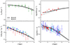 |
Fig. 2. Comparisons between model predictions and observed data of NGC 300. The solid lines correspond to the best-fitting model with a radial inflow of gas (Model B) and the dashed lines to the model without radial inflow (Model A). The left-hand side shows the radial profiles of HI (top) mass and SFR (bottom) surface density, while the right-hand side displays the radial profiles of sSFR (top) and 12 + log (O/H) (bottom). The HI data (see text) are shown by green filled squares. The SFR data are separately denoted as blue filled diamonds (Gogarten et al. 2010), red filled triangles (Williams et al. 2013), and cyan filled circles (Mondal et al. 2019). The sSFR data (see text) are plotted as red filled circles. The 12 + log(O/H) data from the HII regions (Bresolin et al. 2009), BSGs (Kudritzki et al. 2008), and RSGs (Gazak et al. 2015) are shown as red filled asterisks, blue open circles, and cyan filled triangles, respectively. |
As in Kang et al. (2016), the classical χ2 technique was adopted to calculate the best combination of free parameters, which we varied within the range of 0 < a ≤ 3.0, 1.0 ≤ b ≤ 5.0, 0.1 ≤ 0 ≤ c × r/Rd + d ≤ 1.0, and 0 < bout ≤ 1.0. We obtained (a, b, c, d, bout) = (0.16, 3.0, 0.0, 0.1, 0.6), i.e. (τ, υR, bout) = (0.16r/Rd + 3.0 Gyr, −0.1 km s−1, 0.6). The model calculated with these parameters is called Model B. The results corresponding to Model B are plotted as solid lines in Fig. 2. A remarkable agreement is found between the Model B predictions and the NGC 300 observations; that is, the Model B results can simultaneously reproduce the radial observed profiles of the H I gas mass surface density, SFR surface density, sSFR, and 12 + log (O/H).
The best-fitting model of NGC 300 without radial gas inflows in Kang et al. (2016) (Model A) with parameters (τ, υR, bout) = (0.52r/rd + 2.6 Gyr, 0, 0.9) is also plotted in Fig. 2 as a dashed line. We see that Model A is also basically able to reproduce the observed data. The differences between the two models are small, but there are clear systematic trends. The radial gas inflows steepen the present-day radial profiles of HI gas mass surface density, SFR surface density, and metallicity, but flatten the radial sSFR profile. The steeper profiles of gas mass surface density and metallicity predicted by Model B are consistent with the result of Calura et al. (2023). We also note that the central increase in metallicity of Model B is in better agreement with the observations.
υR = − 0.1 km s−1 appears to be a very small value. However, it is supported by a study of 54 local spiral galaxies based on high-sensitivity and high-resolution data of the HI emission line, which finds that the radial inflow velocities are generally small, with an average inflow rate of about −0.3 km s−1 (Di Teodoro & Peek 2021).
The left panel of Fig. 3 shows that, compared to Model A, Model B predicts both delayed and more extended SFHs. The peak of SFR from Model B is shifted by 1 Gyr. The SFR predicted by Model B and Model A are respectively  yr−1 and
  yr−1, consistent with the observed values (see Section 3). The right panel of Fig. 3 shows that the galaxy stellar masses predicted by both Model A and Model B have been steadily increasing to their present-day values. Compared to Model A, Model B forms stars later. The right panel agrees well with the bottom panel of Fig. 17 in Sextl et al. (2023), and based on the galaxy evolution model of Kudritzki et al. (2021) led to the conclusion that most galaxy stellar masses had been assembled in the last 10 Gyr. Figure 3 indicates that the radial gas inflows help to sustain star formation in local spirals, at least in NGC 300.
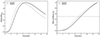 |
Fig. 3. SFH (left) and stellar mass growth history (right) of NGC 300 predicted by Model A (dashed line) and Model B (solid line). SFH is normalised to its maximum value, while stellar mass is normalised to its present-day value. The dotted line in the right panel denotes when the stellar mass achieves 50% of its final value. |
An additional test of our model is obtained by a comparison with the observed mean metallicities for the entire stellar population as derived from the photometric analysis of colour-magnitude diagrams (CMD) in Gogarten et al. (2010). The comparison is carried out in Fig. 4. The model mass-weighted average stellar metallicity at galactocentric radius r and time tg is calculated as (Pagel 1997; Kang et al. 2021)
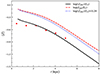 |
Fig. 4. Radial distribution of the mean metallicity of the entire stellar population. Observations obtained from the photometric analysis of colour-maginitude diagrams (CMD, Gogarten et al. 2010) are shown as red circles and the Model B prediction is displayed as the black solid line. The Model B predicted metallicity of the ISM and the very young stars is additionally shown as the red dashed curve. For comparison purposes, the blue dotted curve represents the black curve shifted by +0.24 dex. |
 (17)
(17)
Given the uncertainties of the purely photometric diagnostics, the agreement is quite compelling. We note the Model B predicted metallicity average over all different stellar ages is about  lower than that of the present-day ISM and the very young stellar population. This agrees with cosmological simulations and corresponding chemical evolution models (Finlator & Davé 2008; Pipino et al. 2014; Peng & Maiolino 2014, etc.) and the observational work (e.g. Halliday et al. 2008; Fraser-McKelvie et al. 2022). Based on analysing the integrated stellar population absorption line spectra of ∼200 000 star-forming galaxies in the Sloan Digital Sky Survey, Sextl et al. (2023) also derived that, for a galaxy with stellar mass (log(M*/M⊙) ∼ 9.3), the metallicity difference between the young stellar population and average metallicity is about
  . In addition, we find that the Model B predicted stellar metallicity gradient exhibits a steeper slope compared to the gas-phase gradient, which aligns with previous statistical findings from observational studies (Lian et al. 2018b; Sánchez-Blázquez 2020, and reference therein).
An additional important test of our galaxy evolution model is the prediction with respect to the mass-metallicity relationship (MZR) of star-forming galaxies. This is a key result of a comprehensive spectroscopic project which revealed a tight relationship between the metallicity of the young stellar population and total galaxy stellar mass. Figure 5 displays the latest results obtained from the analysis of individual supergiant stars (Kudritzki et al. 2024) and the stellar population synthesis studies of young stellar populations in SDSS (Sextl et al. 2023) and TYPHOON (Sextl et al. 2024) local star-forming galaxies. The Model B data point (![Mathematical equation: $ \rm [Z]_{\mathrm{NGC300}}\,=\,-0.2335 $](/articles/aa/full_html/2025/09/aa54108-25/aa54108-25-eq49.gif) , the present-day predicted metallicity at a radius r = 0.4R25 as for all galaxies with a metallicity gradient in this plot) fits very nicely on the relationship.
, the present-day predicted metallicity at a radius r = 0.4R25 as for all galaxies with a metallicity gradient in this plot) fits very nicely on the relationship.
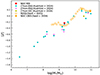 |
Fig. 5. Mass-metallicity relationship of star-forming galaxies. The prediction by Model B shown as a red solid star is compared with observations of a large sample of galaxies. Solid circles refer to the stellar metallicity derived from spectroscopy of individual blue supergiants (cyan), red supergiants (pink), and super star clusters (yellow) (see Kudritzki et al. 2024, and references therein). The open orange diamonds represent the result of integrated galaxy spectra of young stellar population for 250 000 SDSS star-forming galaxies by using a stellar population synthesis technique (Sextl et al. 2023), while the orange solid diamonds denotes the analysis of the spatially resolved young stellar population synthesis study (Sextl et al. 2024). |
A crucial aspect of galaxy evolution is the change in the specific SFR. Figure 6 plots the time evolution of sSFR radial profiles predicted by Model B (solid line) and Model A (dashed line). The values of sSFR are high at early times, and the radial profile is nearly flat. As NGC 300 evolves, the initially flat sSFR gradient becomes steeper due to the gas exhaustion of the inner region of the galaxy. This trend is consistent with the model results obtained by Belfiore et al. (2019). In addition, compared to Model A, Model B predicted sSFR values are higher during the whole evolution history of NGC 300. Radial gas inflows create higher star formation activity. Finally, the model B predicted present-day sSFR profile (i.e. at 13.5 Gyr, black solid line) agrees well with the observed profile derived by using (FUV − K) colours (Muñoz-Mateos et al. 2007). We note that the inclusion of radial gas inflows contributes to bringing the model predicted present-day sSFR profile much closer to the observations of NGC 300 (see the top right panel of Fig. 2) because the radial gas inflows provide more gas in the inner regions at later times.
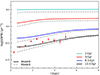 |
Fig. 6. Cosmic time evolution of sSFR radial profiles. The solid lines in different colours represent Model B at 1 Gyr (cyan), 3 Gyr (red), 8.5 Gyr (blue), and 13.5 Gyr (present-day, black). The corresponding results by Model A are shown as grey dashed lines. The red filled circles are the observed data, the same as those in the top right panel of Fig. 2. |
The sSFR of NGC 300 predicted by Model B and Model A are  and −10.127, respectively. They agree well with the observed values (see Section 3) and also fit very nicely on the relationship with stellar mass obtained by xGASS and xCOLDGASS surveys, as shown in Fig. 7.
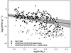 |
Fig. 7. Specific SFR as a function of stellar mass, for the Model B predicted sSFR for NGC 300 (red solid star) and for the observed sSFR of xGASS and xCOLDGASS (Saintonge et al. 2017; Catinella et al. 2018). The solid line refers to the star-forming galaxy main sequence, and the grey shaded region represents the 1σ deviation (Eq. (2) in Catinella et al. 2018). Black filled circles refer to the observed SFR in nearby galaxies from xGASS and xCOLDGASS detections, while the grey filled circles denote non-detections in both xGASS and xCOLDGASS. |
Figure 8 shows the time evolution of the radial metallicity profiles as predicted by Model B (solid line) and Model A (dashed line). The model starts at very low metallicity and with a strong metallicity gradient. Then, while the metallicity increases the gradient becomes flatter. This agrees well with one set of models and simulations (e.g. Boissier & Prantzos 2000; Mollá & Díaz 2005; Pilkington et al. 2012; Minchev et al. 2018; Vincenzo & Kobayashi 2018; Acharyya et al. 2025), but is in tension with several alternative approaches (e.g. Chiappini et al. 2001; Spitoni et al. 2013; Mott et al. 2013; Schönrich & McMillan 2017; Sharda et al. 2021; Graf et al. 2024). In addition, at early times the radial gas inflows flatten the metallicity gradient, whereas at later times they steepen the gradient. This is mainly due to the fact that, at early stages of evolution, the radial gas inflows dilute the metallicity. while at later times the radial gas inflows facilitate star formation and then enrich the metallicity.
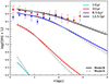 |
Fig. 8. Cosmic time evolution of metallicity radial profiles. The solid lines in different colours represent Model B at 1 Gyr (cyan), 3 Gyr (red), 8.5 Gyr (blue), and 13.5 Gyr (present-day, black). The corresponding results predicted by Model A are shown as grey dashed lines. The red solid circles are the binned metallicity for HII regions from Bresolin et al. (2009), BSGs from Kudritzki et al. (2008), and RSGs from Gazak et al. (2015), while the blue solid diamonds denote the binned metallicity of PNe from Stasińska et al. (2013). |
As already demonstrated by Figure 2, the present-day metallicity of the young stellar population and ISM is reproduced well by our model. Now we also add the PNe studied by Stasińska et al. (2013) (see also Magrini et al. 2016 for construction of radial bins). With an average age of the PNe progenitors of 5 Gyr, it is interesting to compare with the model metallicity at 8.5 Gyr. Except for the two outer bins, the agreement is very good. As already discussed by Stasińska et al. (2013), the oxygen abundance of these outer PNe might be affected by nucleosynthesis in the AGB PNe progenitors.
5. Conclusions
NGC 300 as a well-studied isolated, bulgeless, and low-mass disc galaxy is ideally suited for an investigation of galaxy evolution. In this work, we built a bridge for NGC 300 between its observed properties and its evolution history by constructing a chemical evolution model. The main improvement of the model in this work is the inclusion of radial gas inflows. In addition, we extended the comparison and fit with the observations by adding the results of extensive non-LTE spectroscopy of very young massive stars.
Our model simultaneously reproduces the observed radial profiles of HI gas mass surface density, SFR surface density, sSFR, as well as gas-phase, young stars, and mean stellar metallicity, and allows us to assess the effects of radial gas flows. While the radial flow velocity is very low, ∼−0.1 km/s, it is sufficient to slightly steepen the HI gas mass and SFR surface density profile. It flattens the radial profile of sSFR significantly bringing it closer to the observations. The inclusion of radial inflows leads to increasing star formation along the disc and potentially helping to sustain star formation in local spiral arms.
The effects of radial gas inflows on the present-day radial metallicity distribution are small, but the predicted influencing of the metallicity gradient when going back in time is significantly enhanced. The model predicted present-day metallicity fits nicely on the observed mass-metallicity relationship of star-forming galaxies. It also agrees with the star-forming galaxy main sequence.
Acknowledgments
We thank the anonymous referee for constructive comments and suggestions, which improved the quality of our work greatly. Xiaoyu Kang and Fenghui Zhang are supported by the Basic Science Centre project of the National Natural Science Foundation (NSF) of China (No. 12288102), the National Key R&D Program of China with (Nos. 2021YFA1600403 and 2021YFA1600400), the International Centre of Supernovae, Yunnan Key Laboratory (No. 202302AN360001), the basic research program of Yunnan Province (No. 202401AT070142). Rolf Kudritzki and Xiaoyu Kang acknowledge support by the Munich Excellence Cluster Origins and the Munich Instititute for Astro-, Particle and Biophysics (MIAPbP) both funded by the Deutsche Forschungsgemeinschaft (DFG, German Research Foundation) under the German Excellence Strategy EXC-2094 390783311. Xiaoyu Kang thanks Xu Kong in University of Science and Technology of China for helpful suggestions during revision.
References
- Acharyya, A., Peeples, M. S., Tumlinson, J., et al. 2025, ApJ, 979, 129 [Google Scholar]
- Asplund, M., Grevesse, N., Sauval, A. J., & Scott, P. 2009, ARA&A, 47, 481 [NASA ADS] [CrossRef] [Google Scholar]
- Belfiore, F., Vincenzo, F., Maiolino, R., et al. 2019, MNRAS, 487, 456 [NASA ADS] [CrossRef] [Google Scholar]
- Binder, B., Williams, B. F., Eracleous, M., et al. 2012, ApJ, 758, 15 [Google Scholar]
- Binder, B. A., Williams, R., Payne, J., et al. 2024, ApJ, 969, 97 [Google Scholar]
- Bird, J. C., Kazantzidis, S., & Weinberg, D. H. 2012, MNRAS, 420, 913 [NASA ADS] [CrossRef] [Google Scholar]
- Bland-Hawthorn, J., Vlajić, M., Freeman, K. C., et al. 2005, ApJ, 629, 239 [Google Scholar]
- Boissier, S., & Prantzos, N. 2000, MNRAS, 312, 398 [Google Scholar]
- Bresolin, F., Gieren, W., Kudritzki, R.-P., et al. 2009, ApJ, 700, 309 [NASA ADS] [CrossRef] [Google Scholar]
- Bresolin, F., Kudritzki, R.-P., & Urbaneja, M. A. 2022, ApJ, 940, 32 [NASA ADS] [CrossRef] [Google Scholar]
- Calura, F., Palla, M., Morselli, L., et al. 2023, MNRAS, 523, 2351 [NASA ADS] [CrossRef] [Google Scholar]
- Carr, C., Johnston, K. V., Laporte, C. F. P., et al. 2022, MNRAS, 516, 5067 [NASA ADS] [CrossRef] [Google Scholar]
- Casasola, V., Bianchi, S., Magrini, L., et al. 2022, A&A, 668, A130 [NASA ADS] [CrossRef] [EDP Sciences] [Google Scholar]
- Catinella, B., Saintonge, A., Janowiecki, S., et al. 2018, MNRAS, 476, 875 [NASA ADS] [CrossRef] [Google Scholar]
- Chang, R. X., Hou, J. L., Shen, S. Y., & Shu, C. G. 2010, ApJ, 722, 380 [NASA ADS] [CrossRef] [Google Scholar]
- Chen, Q.-H., Grasha, K., Battisti, A. J., et al. 2023, MNRAS, 519, 4801 [NASA ADS] [CrossRef] [Google Scholar]
- Chiappini, C., Matteucci, F., & Romano, D. 2001, ApJ, 554, 1044 [NASA ADS] [CrossRef] [Google Scholar]
- Cohen, R. E., McQuinn, K. B. W., Murray, C. E., et al. 2024, ApJ, 975, 42 [Google Scholar]
- Dalcanton, J. J., Yoachim, P., & Bernstein, R. A. 2004, ApJ, 608, 189 [NASA ADS] [CrossRef] [Google Scholar]
- Dalcanton, J. J., Williams, B. F., Seth, A. C., et al. 2009, ApJS, 183, 67 [Google Scholar]
- Daniel, K. J., & Wyse, R. F. G. 2015, MNRAS, 447, 3576 [NASA ADS] [CrossRef] [Google Scholar]
- Davies, B., Kudritzki, R. P., Lardo, C., et al. 2017, ApJ, 847, 112 [Google Scholar]
- Di Teodoro, E. M., & Peek, J. E. G. 2021, ApJ, 923, 220 [NASA ADS] [CrossRef] [Google Scholar]
- Edvardsson, B., Andersen, J., Gustafsson, B., et al. 1993, A&A, 500, 391 [NASA ADS] [Google Scholar]
- Feuillet, D. K., Frankel, N., Lind, K., et al. 2019, MNRAS, 489, 1742 [Google Scholar]
- Finlator, K., & Davé, R. 2008, MNRAS, 385, 2181 [NASA ADS] [CrossRef] [Google Scholar]
- Frankel, N., Sanders, J., Rix, H.-W., et al. 2019, ApJ, 884, 99 [NASA ADS] [CrossRef] [Google Scholar]
- Fraser-McKelvie, A., Cortese, L., Groves, B., et al. 2022, MNRAS, 510, 320 [Google Scholar]
- Gazak, J. Z., Kudritzki, R., Evans, C., et al. 2015, ApJ, 805, 182 [NASA ADS] [CrossRef] [Google Scholar]
- Gieren, W., Pietrzyński, G., Soszyński, I., et al. 2005, ApJ, 628, 703 [Google Scholar]
- Gogarten, S. M., Dalcanton, J. J., Williams, B. F., et al. 2010, ApJ, 712, 858 [NASA ADS] [CrossRef] [Google Scholar]
- Goswami, S., Slemer, A., Marigo, P., et al. 2021, A&A, 650, A203 [NASA ADS] [CrossRef] [EDP Sciences] [Google Scholar]
- Graf, R. L., Wetzel, A., Bailin, J., et al. 2024, ApJ, submitted, [arXiv:2410.21377] [Google Scholar]
- Grisoni, V., Spitoni, E., & Matteucci, F. 2018, MNRAS, 481, 2570 [NASA ADS] [Google Scholar]
- Halle, A., Di Matteo, P., Haywood, M., et al. 2015, A&A, 578, A58 [NASA ADS] [CrossRef] [EDP Sciences] [Google Scholar]
- Halliday, C., Daddi, E., Cimatti, A., et al. 2008, A&A, 479, 417 [NASA ADS] [CrossRef] [EDP Sciences] [Google Scholar]
- Haywood, M. 2008, MNRAS, 388, 1175 [NASA ADS] [CrossRef] [Google Scholar]
- Haywood, M., Snaith, O., Lehnert, M. D., et al. 2019, A&A, 625, A105 [NASA ADS] [CrossRef] [EDP Sciences] [Google Scholar]
- Helou, G., Roussel, H., Appleton, P., et al. 2004, ApJS, 154, 253 [NASA ADS] [CrossRef] [Google Scholar]
- Hirschmann, M., De Lucia, G., & Fontanot, F. 2016, MNRAS, 461, 1760 [Google Scholar]
- Ho, I.-T., Kudritzki, R.-P., Kewley, L. J., et al. 2015, MNRAS, 448, 2030 [Google Scholar]
- Kang, X., Zhang, F., Chang, R., Wang, L., & Cheng, L. 2016, A&A, 585, A20 [NASA ADS] [CrossRef] [EDP Sciences] [Google Scholar]
- Kang, X., Chang, R., Kudritzki, R.-P., et al. 2021, MNRAS, 502, 1967 [NASA ADS] [CrossRef] [Google Scholar]
- Kang, X., Kudritzki, R.-P., & Zhang, F. 2023, A&A, 679, A83 [NASA ADS] [CrossRef] [EDP Sciences] [Google Scholar]
- Karachentsev, I. D., & Kaisina, E. I. 2013, AJ, 146, 46 [NASA ADS] [CrossRef] [Google Scholar]
- Karachentsev, I. D., Grebel, E. K., Sharina, M. E., et al. 2003, A&A, 404, 93 [CrossRef] [EDP Sciences] [Google Scholar]
- Kauffmann, G., White, S. D. M., & Guiderdoni, B. 1993, MNRAS, 264, 201 [Google Scholar]
- Khoperskov, S., Di Matteo, P., Haywood, M., et al. 2020, A&A, 638, A144 [NASA ADS] [CrossRef] [EDP Sciences] [Google Scholar]
- Kroupa, P., Tout, C. A., & Gilmore, G. 1993, MNRAS, 262, 545 [NASA ADS] [CrossRef] [Google Scholar]
- Kruijssen, J. M. D., Schruba, A., Chevance, M., et al. 2019, Nature, 569, 519 [NASA ADS] [CrossRef] [Google Scholar]
- Krumholz, M. R. 2014, Phys. Rep., 539, 49 [Google Scholar]
- Kubryk, M., Prantzos, N., & Athanassoula, E. 2013, MNRAS, 436, 1479 [NASA ADS] [CrossRef] [Google Scholar]
- Kubryk, M., Prantzos, N., & Athanassoula, E. 2015, A&A, 580, A126 [NASA ADS] [CrossRef] [EDP Sciences] [Google Scholar]
- Kudritzki, R.-P., Urbaneja, M. A., Bresolin, F., et al. 2008, ApJ, 681, 269 [NASA ADS] [CrossRef] [Google Scholar]
- Kudritzki, R.-P., Ho, I.-T., Schruba, A., et al. 2015, MNRAS, 450, 342 [Google Scholar]
- Kudritzki, R.-P., Teklu, A. F., Schulze, F., et al. 2021, ApJ, 910, 87 [NASA ADS] [CrossRef] [Google Scholar]
- Kudritzki, R.-P., Urbaneja, M. A., Bresolin, F., et al. 2024, ApJ, 977, 217 [Google Scholar]
- Lacey, C. G., & Fall, S. M. 1985, ApJ, 290, 154 [NASA ADS] [CrossRef] [Google Scholar]
- Larson, R. B. 1972, Nature, 236, 21 [NASA ADS] [CrossRef] [Google Scholar]
- Larson, R. B. 1974, MNRAS, 169, 229 [NASA ADS] [CrossRef] [Google Scholar]
- Larson, R. B. 1976, MNRAS, 176, 31 [NASA ADS] [CrossRef] [Google Scholar]
- Leroy, A. K., Walter, F., Brinks, E., et al. 2008, AJ, 136, 2782 [Google Scholar]
- Lian, J., Thomas, D., & Maraston, C. 2018a, MNRAS, 481, 4000 [Google Scholar]
- Lian, J., Thomas, D., Maraston, C., et al. 2018b, MNRAS, 476, 3883 [NASA ADS] [CrossRef] [Google Scholar]
- Lian, J., Zasowski, G., Hasselquist, S., et al. 2022, MNRAS, 511, 5639 [NASA ADS] [CrossRef] [Google Scholar]
- Liu, C., Kudritzki, R.-P., Zhao, G., et al. 2022, ApJ, 932, 29 [NASA ADS] [CrossRef] [Google Scholar]
- Loebman, S. R., Debattista, V. P., Nidever, D. L., et al. 2016, ApJ, 818, L6 [NASA ADS] [CrossRef] [Google Scholar]
- Magrini, L., Stanghellini, L., & Villaver, E. 2009, ApJ, 696, 729 [NASA ADS] [CrossRef] [Google Scholar]
- Magrini, L., Coccato, L., Stanghellini, L., et al. 2016, A&A, 588, A91 [NASA ADS] [CrossRef] [EDP Sciences] [Google Scholar]
- Matteucci, F. 2021, A&A Rev., 29, 5 [NASA ADS] [CrossRef] [Google Scholar]
- Matteucci, F., & Francois, P. 1989, MNRAS, 239, 885 [Google Scholar]
- Mayor, M., & Vigroux, L. 1981, A&A, 98, 1 [NASA ADS] [Google Scholar]
- Minchev, I., & Famaey, B. 2010, ApJ, 722, 112 [Google Scholar]
- Minchev, I., Anders, F., Recio-Blanco, A., et al. 2018, MNRAS, 481, 1645 [NASA ADS] [CrossRef] [Google Scholar]
- Mollá, M., & Díaz, A. I. 2005, MNRAS, 358, 521 [CrossRef] [Google Scholar]
- Mondal, C., Subramaniam, A., & George, K. 2019, J. Astrophys. Astron., 40, 35 [NASA ADS] [CrossRef] [Google Scholar]
- Mott, A., Spitoni, E., & Matteucci, F. 2013, MNRAS, 435, 2918 [Google Scholar]
- Moustakas, J., Kennicutt, R. C., Tremonti, C. A., et al. 2010, ApJS, 190, 233 [NASA ADS] [CrossRef] [Google Scholar]
- Muñoz-Mateos, J. C., Gil de Paz, A., Boissier, S., et al. 2007, ApJ, 658, 1006 [Google Scholar]
- Nantais, J. B., Huchra, J. P., Barmby, P., et al. 2010, AJ, 139, 1178 [Google Scholar]
- Olsen, K. A. G., Miller, B. W., Suntzeff, N. B., et al. 2004, AJ, 127, 2674 [Google Scholar]
- Pagel, B. E. J. 1997, Nucleosynthesis and Chemical Evolution of Galaxies (Cambridge, UK: Cambridge University Press), 392 [Google Scholar]
- Peng, Y.-J., & Maiolino, R. 2014, MNRAS, 443, 3643 [NASA ADS] [CrossRef] [Google Scholar]
- Pilkington, K., Few, C. G., Gibson, B. K., et al. 2012, A&A, 540, A56 [NASA ADS] [CrossRef] [EDP Sciences] [Google Scholar]
- Pilyugin, L. S., Grebel, E. K., & Kniazev, A. Y. 2014, AJ, 147, 131 [NASA ADS] [CrossRef] [Google Scholar]
- Pipino, A., Lilly, S. J., & Carollo, C. M. 2014, MNRAS, 441, 1444 [NASA ADS] [CrossRef] [Google Scholar]
- Pointon, S. K., Kacprzak, G. G., Nielsen, N. M., et al. 2019, ApJ, 883, 78 [NASA ADS] [CrossRef] [Google Scholar]
- Portinari, L., & Chiosi, C. 2000, A&A, 355, 929 [NASA ADS] [Google Scholar]
- Prochaska, J. X., Werk, J. K., Worseck, G., et al. 2017, ApJ, 837, 169 [CrossRef] [Google Scholar]
- Quillen, A. C., Minchev, I., Bland-Hawthorn, J., et al. 2009, MNRAS, 397, 1599 [NASA ADS] [CrossRef] [Google Scholar]
- Recchi, S., Spitoni, E., Matteucci, F., et al. 2008, A&A, 489, 555 [NASA ADS] [CrossRef] [EDP Sciences] [Google Scholar]
- Romano, D., Karakas, A. I., Tosi, M., et al. 2010, A&A, 522, A32 [NASA ADS] [CrossRef] [EDP Sciences] [Google Scholar]
- Roškar, R., Debattista, V. P., Stinson, G. S., et al. 2008, ApJ, 675, L65 [Google Scholar]
- Saintonge, A., Catinella, B., Tacconi, L. J., et al. 2017, ApJS, 233, 22 [Google Scholar]
- Sánchez Almeida, J., Elmegreen, B. G., Muñoz-Tuñón, C., et al. 2014, A&A Rev., 22, 71 [CrossRef] [Google Scholar]
- Sánchez-Blázquez, P. 2020, IAU General Assembly, 261 [Google Scholar]
- Schmidt, M. 1963, ApJ, 137, 758 [Google Scholar]
- Schönrich, R., & Binney, J. 2009, MNRAS, 396, 203 [Google Scholar]
- Schönrich, R., & McMillan, P. J. 2017, MNRAS, 467, 1154 [NASA ADS] [Google Scholar]
- Sellwood, J. A., & Binney, J. J. 2002, MNRAS, 336, 785 [Google Scholar]
- Sextl, E., Kudritzki, R.-P., Weller, J., et al. 2021, ApJ, 914, 94 [CrossRef] [Google Scholar]
- Sextl, E., Kudritzki, R.-P., Zahid, H. J., et al. 2023, ApJ, 949, 60 [NASA ADS] [CrossRef] [Google Scholar]
- Sextl, E., Kudritzki, R.-P., Burkert, A., et al. 2024, ApJ, 960, 83 [Google Scholar]
- Sharda, P., Krumholz, M. R., Wisnioski, E., et al. 2021, MNRAS, 502, 5935 [NASA ADS] [CrossRef] [Google Scholar]
- Spitoni, E., & Matteucci, F. 2011, A&A, 531, A72 [NASA ADS] [CrossRef] [EDP Sciences] [Google Scholar]
- Spitoni, E., Matteucci, F., & Marcon-Uchida, M. M. 2013, A&A, 551, A123 [NASA ADS] [CrossRef] [EDP Sciences] [Google Scholar]
- Spitoni, E., Calura, F., Mignoli, M., et al. 2020, A&A, 642, A113 [EDP Sciences] [Google Scholar]
- Spitoni, E., Verma, K., Silva Aguirre, V., et al. 2021a, A&A, 647, A73 [EDP Sciences] [Google Scholar]
- Spitoni, E., Calura, F., Silva Aguirre, V., et al. 2021b, A&A, 648, L5 [NASA ADS] [CrossRef] [EDP Sciences] [Google Scholar]
- Stanghellini, L., Magrini, L., Casasola, V., et al. 2014, A&A, 567, A88 [NASA ADS] [CrossRef] [EDP Sciences] [Google Scholar]
- Stasińska, G., Peña, M., Bresolin, F., et al. 2013, A&A, 552, A12 [NASA ADS] [CrossRef] [EDP Sciences] [Google Scholar]
- Thon, R., & Meusinger, H. 1998, A&A, 338, 413 [NASA ADS] [Google Scholar]
- Tinsley, B. M., & Larson, R. B. 1978, ApJ, 221, 554 [Google Scholar]
- Tremonti, C. A., Heckman, T. M., Kauffmann, G., et al. 2004, ApJ, 613, 898 [Google Scholar]
- van den Bergh, S. 1962, AJ, 67, 486 [Google Scholar]
- Vincenzo, F., & Kobayashi, C. 2018, MNRAS, 478, 155 [NASA ADS] [CrossRef] [Google Scholar]
- Vincenzo, F., & Kobayashi, C. 2020, MNRAS, 496, 80 [NASA ADS] [CrossRef] [Google Scholar]
- Vincenzo, F., Matteucci, F., Belfiore, F., et al. 2016, MNRAS, 455, 4183 [CrossRef] [Google Scholar]
- Vlajić, M., Bland-Hawthorn, J., & Freeman, K. C. 2009, ApJ, 697, 361 [Google Scholar]
- Westmeier, T., Braun, R., & Koribalski, B. S. 2011, MNRAS, 410, 2217 [Google Scholar]
- Williams, B. F., Dalcanton, J. J., Stilp, A., et al. 2013, ApJ, 765, 120 [NASA ADS] [CrossRef] [Google Scholar]
- Xiang, M., & Rix, H.-W. 2022, Nature, 603, 599 [NASA ADS] [CrossRef] [Google Scholar]
- Yin, J., Hou, J. L., Prantzos, N., et al. 2009, A&A, 505, 497 [NASA ADS] [CrossRef] [EDP Sciences] [Google Scholar]
- Yin, J., Shen, S., & Hao, L. 2023, ApJ, 958, 34 [Google Scholar]
- Zaritsky, D., Kennicutt, R. C., & Huchra, J. P. 1994, ApJ, 420, 87 [NASA ADS] [CrossRef] [Google Scholar]
- Zinchenko, I. A., Just, A., Pilyugin, L. S., et al. 2019, A&A, 623, A7 [NASA ADS] [CrossRef] [EDP Sciences] [Google Scholar]
All Figures
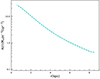 |
Fig. 1. Function A(r) obtained with the best-fitting model of NGC 300 (see Section 4). |
| In the text | |
|
Fig. 2. Comparisons between model predictions and observed data of NGC 300. The solid lines correspond to the best-fitting model with a radial inflow of gas (Model B) and the dashed lines to the model without radial inflow (Model A). The left-hand side shows the radial profiles of HI (top) mass and SFR (bottom) surface density, while the right-hand side displays the radial profiles of sSFR (top) and 12 + log (O/H) (bottom). The HI data (see text) are shown by green filled squares. The SFR data are separately denoted as blue filled diamonds (Gogarten et al. 2010), red filled triangles (Williams et al. 2013), and cyan filled circles (Mondal et al. 2019). The sSFR data (see text) are plotted as red filled circles. The 12 + log(O/H) data from the HII regions (Bresolin et al. 2009), BSGs (Kudritzki et al. 2008), and RSGs (Gazak et al. 2015) are shown as red filled asterisks, blue open circles, and cyan filled triangles, respectively. |
| In the text | |
|
Fig. 3. SFH (left) and stellar mass growth history (right) of NGC 300 predicted by Model A (dashed line) and Model B (solid line). SFH is normalised to its maximum value, while stellar mass is normalised to its present-day value. The dotted line in the right panel denotes when the stellar mass achieves 50% of its final value. |
| In the text | |
|
Fig. 4. Radial distribution of the mean metallicity of the entire stellar population. Observations obtained from the photometric analysis of colour-maginitude diagrams (CMD, Gogarten et al. 2010) are shown as red circles and the Model B prediction is displayed as the black solid line. The Model B predicted metallicity of the ISM and the very young stars is additionally shown as the red dashed curve. For comparison purposes, the blue dotted curve represents the black curve shifted by +0.24 dex. |
| In the text | |
|
Fig. 5. Mass-metallicity relationship of star-forming galaxies. The prediction by Model B shown as a red solid star is compared with observations of a large sample of galaxies. Solid circles refer to the stellar metallicity derived from spectroscopy of individual blue supergiants (cyan), red supergiants (pink), and super star clusters (yellow) (see Kudritzki et al. 2024, and references therein). The open orange diamonds represent the result of integrated galaxy spectra of young stellar population for 250 000 SDSS star-forming galaxies by using a stellar population synthesis technique (Sextl et al. 2023), while the orange solid diamonds denotes the analysis of the spatially resolved young stellar population synthesis study (Sextl et al. 2024). |
| In the text | |
|
Fig. 6. Cosmic time evolution of sSFR radial profiles. The solid lines in different colours represent Model B at 1 Gyr (cyan), 3 Gyr (red), 8.5 Gyr (blue), and 13.5 Gyr (present-day, black). The corresponding results by Model A are shown as grey dashed lines. The red filled circles are the observed data, the same as those in the top right panel of Fig. 2. |
| In the text | |
|
Fig. 7. Specific SFR as a function of stellar mass, for the Model B predicted sSFR for NGC 300 (red solid star) and for the observed sSFR of xGASS and xCOLDGASS (Saintonge et al. 2017; Catinella et al. 2018). The solid line refers to the star-forming galaxy main sequence, and the grey shaded region represents the 1σ deviation (Eq. (2) in Catinella et al. 2018). Black filled circles refer to the observed SFR in nearby galaxies from xGASS and xCOLDGASS detections, while the grey filled circles denote non-detections in both xGASS and xCOLDGASS. |
| In the text | |
|
Fig. 8. Cosmic time evolution of metallicity radial profiles. The solid lines in different colours represent Model B at 1 Gyr (cyan), 3 Gyr (red), 8.5 Gyr (blue), and 13.5 Gyr (present-day, black). The corresponding results predicted by Model A are shown as grey dashed lines. The red solid circles are the binned metallicity for HII regions from Bresolin et al. (2009), BSGs from Kudritzki et al. (2008), and RSGs from Gazak et al. (2015), while the blue solid diamonds denote the binned metallicity of PNe from Stasińska et al. (2013). |
| In the text | |
Current usage metrics show cumulative count of Article Views (full-text article views including HTML views, PDF and ePub downloads, according to the available data) and Abstracts Views on Vision4Press platform.
Data correspond to usage on the plateform after 2015. The current usage metrics is available 48-96 hours after online publication and is updated daily on week days.
Initial download of the metrics may take a while.