| Issue |
A&A
Volume 701, September 2025
|
|
|---|---|---|
| Article Number | A161 | |
| Number of page(s) | 14 | |
| Section | Planets, planetary systems, and small bodies | |
| DOI | https://doi.org/10.1051/0004-6361/202554842 | |
| Published online | 12 September 2025 | |
Ionic emission from and activity evolution in comet C/2020 F3 (NEOWISE): Insights from long-slit spectroscopy and photometry
1
Space sciences, Technologies & Astrophysics Research (STAR) Institute, University of Liège,
Liège,
Belgium
2
Physical Research Laboratory,
Ahmedabad-380009,
India
3
Cadi Ayyad University (UCA), Oukaimeden Observatory (OUCA), Faculté des Sciences Semlalia (FSSM), High Energy Physics, Astrophysics and Geoscience Laboratory (LPHEAG),
Marrakech,
Morocco
4
Université Marie et Louis Pasteur, CNRS, Institut UTINAM (UMR 6213), OSU THETA,
BP 1615,
25010
Besançon Cedex,
France
5
Université Bourgogne Europe, CNRS, Laboratoire Interdisciplinaire Carnot de Bourgogne ICB UMR 6303,
21000
Dijon,
France
6
Indian Institute of Astronomy,
Bangalore-56034,
India
★ Corresponding author: This email address is being protected from spambots. You need JavaScript enabled to view it.
Received:
28
March
2025
Accepted:
28
July
2025
Abstract
Aims. The long-period comet C/2020 F3 (NEOWISE) was the brightest comet in the northern hemisphere since C/1995 O1 (Hale-Bopp). These comets offer a unique opportunity to study their composition and the spatial variation in the different emission in detail. We conducted long-slit low-resolution spectroscopy and narrow-band photometry to track the evolution of its activity and composition during several weeks after perihelion. The images were used to compute the production rates of neutral molecular species and dust, and the spectrum was used to analyse the variation in the emission along the spatial axis in the sunward and anti-sunward directions to detect ionic emission.
Methods. Narrow-band (OH[3090 Å], NH[3362 Å], CN[3870 Å], C2[5140 Å], C3[4062 Å], BC[4450 Å], GC[5260 Å], and RC[7128 Å]) and broad-band (Johnson-Cousins B, V, Rc, Ic) images of comet C/2020 F3 were taken with TRAPPIST-North from 22 July to 10 September 2022 to track the production rates, the evolution of the chemical mixing ratios with solar distance, and the proxy to the dust production (A(0)fρ). A long-slit low-resolution spectrum was obtained on 24 July 2020 using HFOSC on the 2 m HCT at IAO, Hanle. Spectra extracted along the spatial axis in the sunward and anti-sunward directions enabled a comparative analysis of the emission in both directions.
Results. We report production rates and mixing ratios of OH, NH, CN, C2, C3, and NH2 and used the flux density of the forbidden oxygen line to derive the water-production rate. Ionic emission from N2+, CO+, CO2+, and H2O+ was detected at 4 × 10⁴ km to 1 × 10⁵ km from the photocentre in the tail direction. The average N2+/CO+ ratio for the CO+ (3-0) and (2-0) bands measured from the spectrum was (3.0 ± 1.0) × 10–2, which we further refined to (4.8 ± 2.4) × 10–2 using fluorescence modelling techniques. We measured the CO2+/CO+ ratio to be 1.34 ± 0.21. Combining the N2+/CO+ and CO2+/CO+ ratios, we suggest the comet to have formed in the cold mid-outer nebula (~50–70 K). Furthermore, the average rotation period of the comet was calculated to be 7.28 ± 0.79 hours with a CN gas outflow velocity of 2.40 ± 0.25 km/s.
Key words: techniques: photometric / techniques: spectroscopic / comets: general / comets: individual: C/2020 F3
Publisher note: The original typos in the author's name Hmiddouch were corrected on 6 October 2025.
© The Authors 2025
 Open Access article, published by EDP Sciences, under the terms of the Creative Commons Attribution License (https://creativecommons.org/licenses/by/4.0), which permits unrestricted use, distribution, and reproduction in any medium, provided the original work is properly cited.
This article is published in open access under the Subscribe to Open model. This email address is being protected from spambots. You need JavaScript enabled to view it. to support open access publication.
1 Introduction
Comets are celestial bodies composed of ice, dust, and organic compounds. They offer invaluable insights into the early formation stages of our Solar System and its evolution. They serve as time capsules because they preserve clues about the conditions and materials present during the infancy of the Solar System. Consequently, the examination of comets presents a distinctive opportunity to explore the physical and chemical processes that took place during the nascent stages of the formation and evolution of our Solar System.
One of the most intriguing aspects of comets is their dynamic nature, especially during close approaches to the Sun. Comet C/2020 F3 (NEOWISE), hereafter 20F3, is a dynamically old long-period comet1 with a near-parabolic orbit. It was discovered on 27 March 2020 by the NEOWISE space telescope (Mainzer et al. 2014) at magnitude 18.0 when it was at 2.00 au from the Sun. 20F3 was the brightest comet in the northern hemisphere since the comet Hale-Bopp in 1997. The comet reached maximum brightness in early July 2020 with a magnitude of 1, making it bright enough to be visible to the naked eye. The comet with an orbital inclination of 128.92° reached its perihelion on 3 July 2020, at 0.29 au, and its closest approach to Earth occurred on 23 July at a distance of 0.69 au. Strong sodium-doublet emission at 5890 Å was detected at different epochs in July (Lin et al. 2020; Cochran et al. 2020). The H2O+ lines were detected in the visible red wavelength (5800–7400 Å), although they are much weaker than the sodium line, which suggests that the straight red tail reported by numerous observers in mid-July was probably dominated by sodium atoms rather than H2O+ ions (Ye et al. 2020). In support of this, the image2 mentioned by Krishnakumar et al. (2020), taken on 24 July 2020 at the Indian Astronomical Observatory (IAO) site by Dorje Angchuk, clearly illustrates a distinctive blue ion tail. When we consider that the image was taken while the comet was setting, the strong ion tail is seen to be aligned in the eastward direction.
Comets with extensive plasma tails as they approach the Sun closely offer a unique opportunity to study their composition and behaviour. Investigating the relative abundances of key ionic species as a function of the radial distance from the nucleus is one of the best ways to understand the formation and interaction of cometary material with the solar wind (Lutz et al. 1993). These studies can provide essential insights into the physical and chemical processes that occur within the coma and tail of the comet.
Although the detection of major neutral gas species such as CN, C2, C3, and NH2 in the visible range is common, fewer observations have reported the detection of emission from molecular ions such as  , CO+, and H2O+ (eg., Lutz et al. 1993; Wyckoff et al. 1986; Wyckoff & Wehinger 1976; Cochran et al. 2000; Jockers et al. 1987; Kawakita & Watanabe 2002; Cochran 2002; Biver et al. 2018; Cochran & McKay 2018; Korsun et al. 2006; Umbach et al. 1998; Opitom et al. 2019; Venkataramani et al. 2020, and references therein). Furthermore, the detection of emission from
  has been reported for a few comets such as Bradfield (1979 X) and Seargent (1978 XV) (Festou et al. 1982; Weaver et al. 1993), 1P/Halley (Feldman et al. 1986; Wyckoff et al. 1986; Jockers et al. 1987; Umbach et al. 1998), C/2002 C1 (IKEYA-ZHANG) (Cochran 2002), and C/2016 R2 (PanSTARRS3) (Opitom et al. 2019). Most of these detections were made in the near-ultraviolet (NUV) regime, and only a handful of reports were made for
  detections in the optical wavelength range.
We use long-slit low-resolution optical spectroscopy to calculate the production rates of neutral molecular emission and report the detection of ionic species  , CO+,
  , and H2O+ in comet 20F3. This provides new insights into its compositional characteristics. We compare these results with those of radicals observed in the optical spectral range during the same period using the TRAPPIST4-North telescope. Following the introduction in Section 1, Section 2 details our observations and the associated data reduction techniques. The evolution of activity and composition, including the production rates and dust proxies, along with the detection of ionic emission, is described in Section 3.
2 Observations and data reduction
2.1 Photometry (TRAPPIST)
We used the TRAPPIST-North telescope to observe the activity of the bright comet 20F3 post-perihelion for 18 nights, from 22 July (rh = 0.63 au, outbound) to 10 September (rh = 1.61 au, outbound) 2020. We obtained a total of 399 images in various filters. The comet was very bright when we started the observations, with a visual magnitude of about 4.0, and it was also low on the horizon. We had many consecutive good nights, and we were able to follow the drop in activity of the comet day after day before it was no longer visible.
TRAPPIST consists of two 60 cm robotic telescopes dedicated to detecting and characterising exoplanets via the transit method, as well as studying small Solar System bodies such as asteroids and comets (Jehin et al. 2011). TRAPPIST-North (TN; Z53) was installed in 2016 at the Oukaimeden Observatory in Morocco’s Atlas Mountains in collaboration with the Cadi Ayyad University. It is a Ritchey-Chretien telescope with a focal ratio of F/8, mounted on a direct-drive German equatorial mount. TN is equipped with a thermo-electrically cooled deep-depletion 2K × 2K Andor IKON charge-coupled device (CCD) camera, offering a 20′ × 20′ field of view with a high sensitivity. The pixel binning (2×2) was applied, resulting in a plate scale of 1.2″/pixel. We tracked the evolution of the gas production rates of the OH, NH, CN, C3, and C2 species using the HB narrow-band filters (A’Hearn et al. 1995; Farnham et al. 2000; Moulane et al. 2018). Furthermore, we measured the magnitude and the A(0)fρ parameter, which is a proxy to the dust production (A’Hearn et al. 1984), with broad-band filters (B, V, Rc, and Ic) and the blue, green, and red narrow-band dust continuum filters (BC, GC, and RC) (Farnham et al. 2000).
The data were calibrated using standard procedures, with regularly updated master bias, flat, and dark frames. The sky contamination was removed, and the flux was calibrated using frequently updated zero-points. To determine the gas production rates from the HB narrow-band images, we computed the median and radial brightness profiles for the gas filter images and the BC images within an annulus aperture between nucleo-centric distances of 103.6 and 104.1 km. The latter is less affected by cometary gas emission than other dust filters (Farnham et al. 2000). This allowed us to effectively subtract dust contamination from the gas filters using the adjusted flux in the uncontam-inated BC filter and using the dust colour in the narrow-band filters (BC-GC), following the procedure described by Farnham et al. (2000). The surface brightness was then converted into the column density, and the resulting profiles were fitted using a Haser model (Haser 1957; Haser et al. 2020), assuming an outflow velocity of 1 km/s and the effective scale lengths from A’Hearn et al. (1995). Further details on this data reduction process can be found in Moulane et al. (2018), who applied the same method. The Haser model fit was performed within the annulus mentioned above to decrease the aperture effect and lessen dust contamination, and to minimise the effects of the Point Spread Function (PSF) and atmosphere near the optocenter of the comet. The dust contribution is less extended than the gas and peaks at the nucleus. Beyond this distance, the signals, particularly in the OH filter, tend to diminish as a result of the lower signal-to-noise ratio. Fluorescence efficiencies, or g-factors as defined by A’Hearn et al. (1995), were taken from Schleicher’s website5 for the corresponding heliocentric distances to convert the photon density into column densities. Furthermore, we calculated the Afρ parameter within 10 000 km of the nucleus and applied a phase-angle correction using the phase function normalised at θ = 0°, based on the composite phase function described by David Schleicher6, which incorporates elements from Schleicher et al. 1998 and Marcus 2007.
2.2 Long-slit spectroscopy (HCT)
The spectroscopic observations were carried out with the Hanle Faint Object Spectrograph and Camera (HFOSC) mounted on the 2m Himalayan Chandra Telescope (HCT) at the Indian Astronomical Observatory (see Aravind et al. 2022, for further details about the use of the HCT and HFOSC for comet observations). We used a slit that was 11′ long and 1.92″ wide to observe the comet. This slit corresponds to a resolving power of ~1300 and provided a spectral resolution of ~1.45 Å/pixel. The observations were carried out on the night of 24 July 2020 when the comet was at a heliocentric distance of 0.66 au and at a geocentric distance of 0.69 au.
Two spectra of 300 seconds each were obtained with the comet at the centre of the slit oriented east-west (see Figure 1). The spectroscopic standard star Feige 110 was also observed, with a wider slit (15.4″) to avoid light loss, to construct the sensitivity function of the instrument required for the flux calibration. The halogen-lamp spectra, zero-exposure frames, andFeAr spectra were also obtained for the flat fielding, bias subtraction, and wavelength calibration, respectively.
The comet spectroscopic data were reduced and calibrated using self-scripted Python codes and Image Reduction and Analysis Facility (IRAF), following normal long-slit procedures as detailed by Aravind et al. (2022). As a result of the time constraint in obtaining a separate sky frame, the sky spectra were extracted for similar apertures from a standard star frame observed for similar exposure time and similar airmass on the same night. The corresponding sky spectra were used for an effective sky subtraction from the comet spectra.
The preliminary analysis of the 2D spectra of 20F3, as shown in panel a of Figure 2 discovered doublet emission at certain positions in the anti-sunward direction. At the time of observation, the angular difference of the slit and the anti-sunward direction was only 22° in the clockwise direction. Considering the orientation of the ion tail and the possibility of coincidental projection orientation with the slit direction (eastward, see Figure 1), we therefore searched for ionic emission by analysing the emission in spatial directions, both westward (anti-tailward or sunward) and eastward (tailward or anti-sunward). For this reason, we extracted three cometary spectra: at the photocentre (C) and at the two ends of the slit (202″ away from the photo-centre) eastwards (E) and westwards (W), each for an aperture of 30″, from the observed long-slit spectra that correspond to the locations C, E, and W, respectively, as shown in panel b of Figure 2.
The comet spectrum comprises the coma gas emission spectrum and the spectrum of the sunlight scattered by the dust particles. It is therefore necessary to remove the continuum signal in order to obtain the pure gaseous emission. A solar spectrum or a solar analogue spectrum was used to remove the continuum signal. We used the solar-analogue star HD 19445, which was observed using the same instrument under the same settings. The observed solar-analogue spectrum was initially normalised and scaled to the comet continuum flux. A ratio of the polynomial fit to the two spectra (using the continuum windows mentioned in Ivanova et al. 2021) corrected for the redder dust of the comet. Multiplying the scaled solar spectrum by the polynomial ratio gives the comet continuum spectrum, which was then subtracted to extract the pure emission spectrum. The corresponding pure emission spectra extracted from the photocentre and the extreme points of the slit in the anti-tailward and tailward directions marked with the prominent emission detected (for the centre) and dissimilarity regions (for extreme regions) are shown in Figure 3.
Furthermore, to facilitate the computation of the relative abundance of the detected ionic emission along the spatial axis, we used multiple equidistant apertures (1, 2, 3, 4, and 5) of 12″, as shown in Figure 2. The sunward direction was marked to clarify that the multiple apertures were extracted in the tailward (anti-sunward) direction.
The multiple aperture extraction along the spatial axis in the anti-sunward direction shows that the ionic species corresponding to different molecular species start to be visible at about 3σ level (σ being the error in the continuum) for an aperture distance beyond ~35 000 km from the photocentre. The analysis of the column density profile of the main emission (using Equation (4)) shows that the column densities of C3 and NH2 dropped steeply and became negligible beyond a distance of ~20 000 km from the photocentre (see Figure 4). This sharp decline, along with the coincidental orientation of the strong ion tail with the slit direction, facilitated the detection of these species far from the photocentre (see Figure 5).
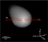 |
Fig. 1 Orientation of the slit overlaid on an HFOSC image at the time of acquisition on 24 July 2020. |
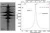 |
Fig. 2 Panel a: 2D spectrum of 20F3. The blue wavelength starts from the top. The white arrows denote the visually noted doublets in the anti-sunward direction. Panel b: various apertures (horizontal bars) for the spectral extraction compared to the comet photon density profile around the nucleus. Ε and W represent the apertures used in the east and west directions, respectively. |
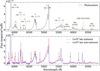 |
Fig. 3 Long-slit spectra of 20F3 observed on 24 July 2020, extracted at photocentre (top panel) and at the extreme regions of the slits in the tailward and anti-tailward directions (bottom panel). The arrows depict the dissimilarity regions for spectra extracted from extreme regions of the slit. |
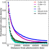 |
Fig. 4 Median column density profiles of the main molecules detected in the spectrum. |
 |
Fig. 5 Detected emission for spectra extracted (a) and (b) at photocentre, and (c) and (d) 105 km in the tailward direction. |
2.3 Haser factor computation
With long-slit spectroscopic observations of comets, only a portion of the total coma is observed. Therefore, the observed flux density of each molecular species must be extrapolated to determine the total flux density for the entire coma. Using the Haser coma outflow model, Fink & Hicks (1996) provided a factor known as the Haser factor, which is the ratio of the total number of molecules within the observed aperture to the total number of molecules in the entire coma. The reciprocal of this factor, the Haser correction, can be used to extrapolate the observed flux density and estimate the molecular abundance in the whole coma. The Haser model assumes a spherically symmetric coma with a uniform outflow of gas. An internet calculator provided by Dave Schleicher on his website7 can compute this factor for a circular aperture centred on the nucleus for a set of molecules (CN, C2, C3,NH, and OH).
We used a rectangular slit, however, which makes it less straightforward to compute the Haser factor for an equivalent circular aperture. In addition, we computed the production rates of NH2 and H2O, for which the Haser factors are not available from Schleicher’s website. We therefore developed a Python code that uses the activity module available within the sbpy package (Mommert et al. 2019) to create a 2D image of the column density from the Haser model and used the photutils package (Bradley et al. 2016) to extract the Haser fraction for any given aperture. We cross-checked our results with the internet calculator mentioned above for circular apertures, and they match in the decimal places with a better approximation.
This code can compute Haser factors for rectangular apertures of user-defined sizes with the comet at the centre and off-centred apertures. Figure 6 illustrates a similar scenario in which the Haser factor calculation of the CN molecule is carried out for an aperture of size of 100″ in a slit of width 1.92″. In this manner, the Haser factor can be computed for any molecule with known scale lengths for a user-defined aperture at a particular geocentric and heliocentric distance.
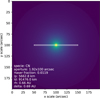 |
Fig. 6 Rectangular slit for which the Haser factor computation was performed from a 2D image of the column density from the Haser model. |
Gas production rates and A(0)fρ parameter of 20F3 (NEOWISE).
3 Results
In this section, we present the light curve in different filters and the evolution of the comet activity and composition after its perihelion passage from photometric observation. We also discuss the results obtained from the spectroscopic observations.
3.1 Photometry
We began the observation of 20F3 three weeks after perihelion on 22 July 2020 (rh = 0.63 au), as it was getting higher in the northern sky, at least 10 degrees above the horizon. We followed its activity with TN until 10 September 2020 (rh = 1.61 au). All species were detected since the first day of observation. As the comet was very bright around perihelion, short exposures were used to avoid saturating the images. The coma did not show any sign of outburst or increase in elongation, which is often associated with disruption of the nucleus at small heliocentric distances.
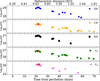 |
Fig. 7 Logarithmic production rates of OH, NH, CN, C3, and C2 detected in 20F3 as a function of time and heliocentric distance. The vertical dashed line indicates the perihelion on 3 July 2020, at 0.29 au. The red mark in each symbol represents the corresponding measurements from the spectroscopic observation. |
3.1.1 Production rates and dust activity
The derived production rates for each detected gas species, the A(0)fρ dust parameter, and their absolute errors are given in Table 1. Their evolution as a function of time and heliocentric distance is shown in Figures 7 and 8.
The maximum activity of the comet was measured on the third night of our observations after perihelion (July 24, rh = 0.67 au), with an OH production rate of (1.08 ± 0.31) × 1029 molec/s. It then decreased rapidly as the comet went away from the Sun. Dave Schleicher (private communication) derived an OH production rate of 1.02 × 1029 molec/s (Jul 28, rh = 0.74 au) from the Lowell Observatory. This result is higher than our measurement of (7.63 ± 1.12) × 1028 molec/s from two days earlier (July 26, rh = 0.71 au). We obtained an OH production rate of (1.80 ± 0.34) × 1028 molec/s on 11 August (rh = 1.05 au), and Schleicher obtained 4.16 × 1028. The aperture around the nucleus was 25 700 km for Schleicher, and we used an annular aperture across 10000 km for our calculations. The difference in the production rates is the result of the different apertures and computation method. Faggi et al. (2021) obtained high-resolution infrared spectra of comet 20F3 in July 2020. They were able to detect many parent species, such as CO, OCS, HCN, C2H2, NH3, NH2, H2CO, CH4, C2H6, and CH3OH. Future work can compare daughter and parent species such as CN and HCN, OH and H2O, C2 and C2H2 or C2H6 and determine whether they agree well, which would then strengthen their links.
Figure 9 shows the evolution of the magnitude in different filters (Β, V, Rc, and Ic broad-band filters) as a function of time compared to the JPL ephemeris magnitude. The standard magnitude model M = M0 + 5 × log(rg) + 2.5 × n × log(rh) was used with the best-fit parameters, where η is the activity index, M0 is the absolute magnitude, and rg and rh are the geocentric and heliocentric distances, respectively. The best-fit parameters we obtained are M0(B) = 12.32, n(B) = 4.22; M0(V) = 11.92, n(V) = 3.85; M0(Rc) = 12.06, n(Rc) = 4.03; and M0(Ic) = 12.18, n(Ic) = 3.53 for Β, V, Rc, and Ic, respectively. The light curve shows no small-scale deviations, indicating that the activity evolution remained stable, with a noticeable fast drop after perihelion.
Figure 10 illustrates the relative abundances of the various daughter species and the dust/gas ratios with respect to CN and OH. Even though the production rate ratios vary slightly over the heliocentric distance range of 0.63–1.61 au, they remain well above or within the range defined by A’Hearn et al. (1995) for comets with a typical carbon composition. We obtained an average value of Log10[Q(C2)/Q(CN)] = 0.14 ± 0.02, which is in the high range of typical values for normal comets (0.06 ± 0.10) as reported by A’Hearn et al. (1995). The mean value of the dust/gas ratio (Log10(A(0)fρ/OH) = –25.42 ± 0.40 and Log10(A(0)fρ/CN) = –23.17 ± 0.11) is also well within the range observed for gas-rich comets. These ratios therefore indicate that comet 20F3 has a typical coma composition with a dust/gas ratios similar to that of typical gas-rich comets.
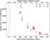 |
Fig. 8 A(0)fρ parameter of 20F3 at 10 000 km from the broad- and narrow-band filters as a function of time and heliocentric distance. |
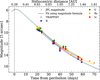 |
Fig. 9 Optical light curve of 20F3 measured within a 5-arcsecond aperture as a function of time and distance to perihelion. The vertical dashed line indicates the perihelion at 0.29 au on 3 July 2020. |
3.1.2 Coma morphology and rotation period
Coma features and jets in the CN narrow-band images were investigated by applying azimedian and rotational (Sekanina & Larson 1984) filtering. The first CN series was obtained during the night starting on 22 July. In azimedian-filtered images, two main jets separated by around 90°, directed north and east on the plane of the sky, are distinguishable. A possible third jet oriented west can be observed in the rotational filtered image. A second series taken the night starting 23 July at the same time in the night shows similar features with a similar orientation, indicating a rotation period close to an alias of 24 h. Observations on the nights starting July 24, 25, and 26 show apparent disconnection between the northern jet and the optocenter, as well as a radial outward translation of the jet feature. This might indicate changes in the activity regions. Jets were observed in our images until mid-August, but cannot be directly linked to the July 22–23 jets, as new jets seem to appear and others fade out between observations.
To obtain the rotation period from the jets, we first performed a Lomb-Scargle periodogram over the different consecutive nights. The periodic analysis was made with the angle between the tangent of the most prominent jet (oriented north when our images were taken; see Figure 11), the optocenter and the (arbitrarily chosen) east on each of the images. Given the difficulty to relate given jets between different nights, the analysis was limited to the nights of July 22 and 23, totalling nine images. The periodogram analysis showed that the best-matching frequencies (above a false-alarm positive of 0.01) are 22.6 h and the aliases are 7.5, 4.5, and 3.8 h. This degeneracy is expected because the observations were made around the same time each night, and the sample only contained images from two nights. The image series of the night of 22 July shows that the spirals rotate by 50° over one hour (see Figure 11), however, which confirms the period of ~7.2 h.
To complement the periodic analysis, the variation in the jet angle was measured over the night in series from the night starting 22 July (totalling 6 images) and 26 July (totalling 12 images). This method yielded periods of 7.91 ± 0.77 hours and 6.65 ± 0.81 hours, respectively. The given values are the average of the measurements on individual images over the night, with the uncertainty as the standard deviation. The obtained periods agree with the two nights and with the periodic analysis. Our measurements are also consistent with the period of 7.8 ± 0.2 h derived by Manzini et al. (2021) from the modelling of the coma dust and with 7.28 ± 0.03 h derived from features in C2 narrow-band images by Drahus et al. (2020).
The associated CN outflow velocity in the plane of the sky was obtained by fitting an Archimedian spiral to the jet, assuming a constant CN outflow velocity. An Archimedean spiral of the form r = bθ, where r and θ are polar coordinates and b determines the spacing between spiral arms, was fitted to the coma. The quantity 2πb corresponds to the projected distance between successive arcs along an axis through the nucleus, representing the distance the gas travels during one nucleus rotation. Based on the known rotation period, the outflow velocity can be estimated. We derived CN outflow velocities of 2.39 ± 0.23 km/s (23 July) and 2.44 ± 0.30 km/s (26 July). The derived velocity is seen to be on the higher side compared to the usually assumed velocity of 1 km/s or that obtained using the relation  (Cochran et al. 2012). This relation apparently might not be applicable to all comets, however. Tseng et al. (2007) reported expansion velocities of up to 2 km/s at 1 au for C/1995 Ol (Hale-Bopp) based on 18 cm OH line profiles, with similarly high velocities observed in lP/Halley and C/1996 B2 (Hyakutake). Following the velocity–distance power law derived for Hale-Bopp by Tseng et al. (2007) to 0.65 au yields a velocity of 2.68 km/s, which is similar to our results for 20F3.
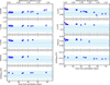 |
Fig. 10 Logarithm of the production rates and dust-to-gas ratios of C/2020 F3 with respect to CN and to OH as a function of time and heliocentric distance. The horizontal dashed blue line and the shaded region represent the mean ratios and range of ratios for comets with typical carbon composition as defined by A’Hearn et al. (1995). The red mark in a few panels represents the corresponding measurements from the spectroscopic observation. The error bars correspond to the 1σ absolute errors. |
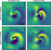 |
Fig. 11 Azimedian (left) and rotational (right) CN narrow-band filtered images selected the night starting 22 July, one hour apart. The images are oriented with north up and east to the left. The red spirals follow the northern jet, which was used for the rotational and velocity analysis. |
3.2 Spectroscopy
The top panel of Figure 3 show that the neutral molecular species (CN, CH, C2, C3, and NH2) are dominant in the spectrum extracted from the photocentre. The spectrum extracted from the tailward region of the cometary coma exhibits differences in emission in multiple areas of the spectrum, however. The absence of certain emission in the anti-tailward directions confirms their cometary origin. Most of the new emission detected in the tailward spectrum, marked in the lower panel of Figure 3, was mainly ionic emission of different molecular species. The following subsections briefly discuss the computation of production rates of the neutral molecular species, the identification of the detected ionic emission, the computation of their column densities, the variation in their abundance ratio along the spatial axis, and their implications.
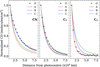 |
Fig. 12 Comparison of Haser model fittings for the observed (O) column densities of CN, C2, and C3 making use of respective scale-lengths defined by A’Hearn et al. (1995) (A), Langland-Shula & Smith (2011) (B), and Cochran et al. (2012) (C). |
3.2.1 Production rates of neutral molecular species
In comet studies, production rates of species such as CN, C2, and C3 usually come from fitting column density profiles with the Haser model (see Aravind et al. (2022) and Langland-Shula & Smith (2011) for details) or from single-aperture spectral extraction with Haser correction (see Aravind et al. (2021) for details). The scale lengths in active comets may vary, however, as already shown in the literature (e.g. Fink et al. 1991; Cochran 1985; Fink & Combi 2004, and references there in). Scale lengths from different studies (e.g. A’Hearn et al. (1995), Cochran et al. (2012), Langland-Shula & Smith (2011)) were chosen to illustrate this situation (see Figure 12) and highlight the limitations of using generic scale lengths to represent the complex and changing chemistry of an active coma.
Developing a custom set of scale lengths for the activity of 20F3 would improve our understanding of the species and complex coma chemistry, but this is beyond the scope of this study, as our goal here is to derive production rates using the most commonly adopted scale lengths to enable a comparison of 20F3 with other comets. In the case of 20F3, although the fit quality of the Haser model varied with the choice of scale lengths, the resulting production rates were generally found to remain consistent within the observational uncertainties.
We used single-aperture spectral extraction to compute the production rates from spectroscopic data along with the equation
 (1)
(1)
where Δ is the geocentric distance in au, g is the fluorescence efficiency (ergs/molecules/s), vout is the outflow velocity assumed to be 1 km/s, and 1d is the scale length of the daughter molecule. Here, the flux in Equation (1) is the total spectral flux density of the molecule of interest within the defined bandpass (taken from Langland-Shula & Smith 2011 and Fink 2009), and HC is the Haser correction, defined as the inverse of the Haser factor. The Haser factor, that is, the ratio of the number of molecules of the emitting species within an arbitrary aperture to the total number of molecules if the aperture were extended to infinity, was computed as described in Section 2.3.
Since the scale-lengths defined by A’Hearn et al. (1995) are widely used to compute the production rates of comets, we also adopted the same values for the molecules CN, C2, and C3 to maintain consistency and ensure uniformity in comparison between different datasets and observational methods. The values were then scaled to  , rh being the heliocentric distance. Although the fluorescence efficiencies of C2 and C3 were taken from A’Hearn et al. (1995) and scaled to
  , the efficiency of CN was obtained by performing a double interpolation in the table provided by Schleicher (2010), which contains the g factor of CN for different heliocentric distances and velocities. The scale length and fluorescence efficiency of the NH2 (0-10-0) band were taken from Fink (2009) and scaled to
  and
and  , respectively (see Table 2 for details).
We also attempted to compute the water-production rate using the spectral flux density of the forbidden oxygen line (hereafter [OI]) at 6300 Å. This approach was used before in many cases (eg., Schultz et al. 1992; Fink & Hicks 1996; Morgenthaler et al. 2001, 2007; McKay et al. 2012; Opitom et al. 2020; McKay et al. 2020). Because the observations are in low-resolution mode here, significant contamination from the sky and the nearby NH2 bands is expected. As mentioned in Section 2.2, the sky contamination was removed effectively, which left us with the NH2 contamination. We followed the method described by Fink (2009) to remove the NH2 contamination, where 0.9 times the spectral flux density of the (0-8-0) NH2 band peak at 6335 Å was subtracted from that of the [OI] 6300 Å line (see Figure 13 for the mentioned peaks and Table 2 for the adopted scale length).
The resulting production rate of oxygen atoms in the (1D) state, Q([OI]), was computed as
![Mathematical equation: $Q\left( {\left[ {OI} \right]} \right) = {4 \over 3}\left( {4\pi {\Delta ^2}{F_{6300}}} \right) \times HC,$](/articles/aa/full_html/2025/09/aa54842-25/aa54842-25-eq18.png) (2)
(2)
where Δ is the geocentric distance in cm, F6300 is the decontaminated spectral flux density of the 6300 Å [OI] line (in photons s–1 cm–2), and HC is the Haser correction to account for the emission that is not encompassed in the aperture (e.g., Morgenthaler et al. 2001; Schultz et al. 1992). Since [ΟΙ] emission is the result of a forbidden transition rather than fluorescence, if all these photons come from O(1D) created during the photodissociation of H2O and its daughter OH, the water-production rate Q(H2O) can be derived from O(1D) production rate using the expression
![Mathematical equation: $Q\left( {{H_2}O} \right) = {{Q\left( {\left[ {OI} \right]} \right)} \over {BR1 + \left( {BR2*BR3} \right)}},$](/articles/aa/full_html/2025/09/aa54842-25/aa54842-25-eq19.png) (3)
(3)
where BR1, BR2, and BR3 were chosen to be 0.05, 0.855, and 0.094, respectively (see Opitom et al. (2020) and references therein). They are the branching ratios for the three reactions
 (i)
(i)
 (ii)
(ii)
 (iii)
(iii)
We used these computation methods to compute the production rates for CN, C2, C3, NH2 and H2O for multiple aperture sizes varying from 90 to 120 arcseconds to minimise any possible effects of quenching within the inner coma (crucial in the case of H2O) and non-uniform slit illumination towards the slit ends. The average of the computed production rates and their standard deviation taken as the 1σ absolute error are listed in Table 3.
The computed production rates of CN, C2, and C3 are comparable to those derived from the TRAPPIST observations, as discussed earlier in Section 3.1. The water-production rate computed in this work from the [OI] line, ~20 days after perihelion, agrees very well with that reported by Combi et al. (2021) from HLy–α observations by SWAN8 onboard SOHO9 and Faggi et al. (2021) from the observations of H2O lines in the near-infrared (NIR) region by the iSHELL instrument on the NASA Infrared Telescope Facility (IRTF) (see Figure 14). The water-production rate calculated using the empirical conversion formula  (Schleicher et al. 1998) is slightly lower side than the other results. A similar discrepancy in the water-production rates between TRAPPIST and SOHO values has previously been highlighted by Opitom et al. (2015), Dello Russo et al. (2016), and Moulane et al. (2023). These inconsistencies between the water-production rates reported from spectroscopic and narrow-band photometric observations might be due to a possible residual NH2 contamination within the [OI] 6300 Å line, differences in adopted scale lengths, and the complexities of coma chemistry.
We inferred that the spectral flux density of the [OI] line can be used to calculate a robust upper limit of water-production rates. Furthermore, the production rate ratios with respect to CN listed in Table 3 classify comet 20F3 as typical in composition according to the definition by A’Hearn et al. (1995).
Scale lengths and fluorescence efficiencies adopted for the different molecules.
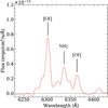 |
Fig. 13 6335 Å NH2 peak used to decontaminate the NH2 contribution in the [OI] 6300 Å line. |
Production rates and rate ratios for the main neutral molecules in 20F3 observed on 24 luly 2020.
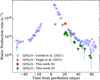 |
Fig. 14 Comparison of water production of 20F3 computed in this work using the 6300 Å [OI] line spectral flux density (S) and OH narrow-band images (P) with those reported by Combi et al. (2021) and Faggi et al. (2021). The error bars correspond to 1σ absolute errors. |
3.2.2 Detected ionic emission and sodium
We detected emission from the ionic species  , CO+,
  , H2O+, and sodium (Nal) in 20F3 while we explored the spatial axis in the tailward direction. The respective emission and the corresponding bands are shown in panel (a) of Figure 15. The identified sodium emission from the sodium doublet at 5889.95 (D2) and 5895.92 Å (D1) originates from the comet and the atmosphere of the Earth. They are indistinguishable at our low spectral resolutions. With the sky contribution for an exposure time of three minutes being minimal for bright comets like C/2020 F3 and having performed proper sky removal, as explained earlier, the remaining observed NaI emission can be considered to be of cometary origin. The bottom panel of Figure 3 shows the excess sodium emission in the tailward direction that confirms its cometary origin. The ionic emission was identified with the help of similar work reported in other publications (eg., Wyckoff & Wehinger 1976; Cochran 2002; Wyckoff et al. 1986, 1999; Venkataramani et al. 2020; Hardy et al. 2023). The steep drop in the column densities of the main neutral species C3 and NH2 in the blue and red range (see Figure 4) facilitated the detection of the ionic species CO+ and H2O+, respectively, far from the nucleus (see Figure 5).
We confirmed the emission from CO+ and H2O+ with the help of the model spectra of CO+ (Rousselot et al. 2024) and the laboratory spectra of H2O+ (Lew 1976), convolved with the instrument profile obtained from the FeAr calibration lamp lines (see panels b and c of Figure 15). It is assumed that excess emission in the tailward spectrum around 5500 Å (see the bottom panel of Figure 3) is due to the H2O+ (10-0) emission at 5469.97, 5479.78 and 5488.78 Å, which was identified with the help of the markings provided by Wyckoff & Wehinger (1976) and the detailed line list provided by Wyckoff et al. (1999).
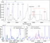 |
Fig. 15 Spectrum of 20F3 extracted from the tailward direction, 1 × 10⁵ km away from the photocentre (a) depicting the detection of ionic emission and a few unidentified emissions; (b) overplotted with the modelled spectrum of CO+ (Rousselot et al. 2024) convolved with the instrument profile, and (c) overplotted with the laboratory spectra of H2O+ (Lew 1976) convolved with the instrument profile. |
3.2.3 Ion column densities and abundance ratios
The column density (N) of an ion, whose electronic transitions are excited by resonance fluorescence, is given by
 (4)
(4)
where F is the integrated band flux density of the cometary ion of interest, g is the fluorescence efficiency, and Ω is the solid angle subtended by the aperture used at the comet. We adopted fluorescence efficiencies (ergs/ion/s) at 1 au of 1.7 × 10⁻¹⁴ and 1.36 × 10⁻¹⁴ for the CO+(3-0) and CO+(2-0) bands, respectively (Rousselot et al. 2024), 2.48 × 10⁻¹³ for the  band (Rousselot et al. 2022) and 2.1 × 10⁻¹⁴ for the H2O+(0-8-0) band (Lutz et al. 1993). In all cases, the fluorescence efficiencies were scaled to the appropriate heliocentric distance (rh), following
  Panel a of Figure 15 clearly shows that the
  band is highly blended with the CN emission, which makes it difficult to extract the actual flux. We only extracted the flux density of the visible emission band head to compute the abundance ratio. Dedicated fluorescence modelling techniques are to be incorporated to estimate the underlying
  within the CN emission band. Table 4 provides the flux densities and their absolute errors for the detected ionic species for an aperture of 12″ at various distances from the photocentre.
The value of N2/CO for the protosolar nebula was calculated to be 0.145 ± 0.048 (Fegley & Prinn 1989; Lodders et al. 2009; Rubin et al. 2015). Since N2 is the least reactive among nitrogen-bearing species and serves as the primary carrier of nitrogen in the solar nebula, a low abundance of elemental nitrogen in a comet must primarily result from the depletion of N2 itself (Feldman et al. 2004). Anderson et al. (2023) asserted that the measured N2/CO ratio is unrelated to the dynamical history of the comet (number of passages into the inner Solar System) and therefore directly represents the volatile composition of the comet. Owen & Bar-Nun (1995) reported that the N2/CO of comets that formed around a temperature of 50 K would be 0.06 if N2/CO is 1 in the solar nebula. Owen & Bar-Nun (1995) also stated that comets forming at higher temperatures, close to the similar ionisation efficiencies and are fully photodissociated in the coma.
We took the importance of this ratio and used
 (5)
(5)
to derive the average  for the (3-0) and (2-0) bands of CO+ (see Table 5 for the ratios computed for an aperture of 12″ at various distances from the photocentre). The variation in the abundance in the spatial direction along the slit was checked for these bands, and it was found to be consistent within the error bars for nucleocentric distances varying from ~4 × 10⁴ km to ~1 × 10⁵ km. The abundance ratio,
  , measured for the same distances, however, varied from ~0.04 to ~0.15, which is comparable to the values reported by Lutz et al. (1993), but lower by a factor of 10 than those reported by Biermann et al. (1982) based on photochemical models. As mentioned before, since the
  flux density is not measured for its entire wavelength range, we incorporated the fluorescence modelling technique to obtain a better approximation of the ratio. The details are discussed in Section 3.2.5.
Observed ion flux densities (ergs/cm2/s).
Observed ion abundance ratios.
3.2.4 Detection of  and unidentified emission
The analysis of the tailward spectrum facilitated the identification of a few previously reported unidentified emission. The unidentified emission reported by Wyckoff et al. (1999) for comet Hyakutake (C/1996 B2) at locations 5273, 5289, 5333, and 6003 Å were also observed in 20F3 (see panel a of Figure 15). Due to the availability of the very high-resolution emission atlas for 20F3 (Cambianica et al. 2021) and the comet line atlas provided by Hardy et al. (2023), the previously unidentified emission observed at 5273,5333, and 6003 Å are identified as possibly belonging to the C2 bands, while the emission at 5289 Å possibly belongs to NH2. Subsequently, Bodewits et al. (2019) demonstrated that many of the previously unidentified emission described by Wyckoff et al. (1999) can be attributed to transitions originating from the higher vibrational levels of H2O+ (A2A1 - X2 B1).
In addition, only a small fraction of known comets with a significant detection of  emission were known before from ground-based observations. Comet 1P/Halley was one major candidate to have multiple reports of emission from
  in the optical regime. While Umbach et al. (1998) identified
  emission in comet Halley within the wavelength range of 3660–3700 Å, Jockers et al. (1987) detected
  emission within the same range, but noted an unidentified emission at 4130 Å. Wyckoff et al. (1986) later confirmed the 4130 Å emission to be
  by comparing it with a laboratory spectrum by Smyth (1931), and they additionally reported
  emission at around 4340 Å. Later, Cochran (2002) expanded these findings by detecting
  emission in comet Ikeya-Zhang within the range of 3400–3700 Å and also at 4130 Å.
Apparently, Lutz et al. (1993) observed ionic emission in comet Bradfield 1987, but did not report significant emission at 4130 Å. More recently, Opitom et al. (2019) reported the detection of  in Comet C/2016 R2 within the wavelength range of 3500–3660 Å. We also identified emission of
  around 4130 Å in the high-resolution UVES spectra of comet C/2016 R2 and in the tail spectrum of comet C/2002 T7 (LINEAR) in a current effort to build an atlas of cometary lines that is still in progress (Hardy et al. 2023). The absence of this emission in the low-resolution spectrum of C/2016 R2 reported by Venkataramani et al. (2020) (see Figure 17), in contrast to its presence in the high-resolution spectra, might be attributed to the difference in the heliocentric distance at the time of observation. The comet was at a comparatively smaller heliocentric distance during the observations reported by Opitom et al. (2019), which may have contributed to the emergence of the emission feature. More precisely, the only lines present in that region are weak
  bands that we identified in comets C/2016 R2 and C/2002 T7 at exactly 4108.45 (3,8), 4109.45 (2,5), 4121.58 (4,7), 4123.29 (3,6), 4138.76 , and 4139.52 Å. This matches the laboratory
  line lists of Mrozowski (1947b,a), and Kim (1999). At the low-resolution of the 20F3 spectrum in the tail direction, these bands are seen to merge to give a broader feature similar to the band observed in 20F3. Moreover, the absence of any strong bands of CO+ (Rousselot et al. 2024), CN bands (confirmed using the planetary spectrum generator (PSG, Villanueva et al. 2018, 2022)) and C3 emission (diminished at this distance from the photocentre, as shown in Figure 4) in this region, this feature around 4130 Å can be attributed to
  . In comet C/2002 C1 (Ikeya-Zhang), which had strong emission from CN, C3 and CO+, Cochran (2002) identified this broad feature to be
  .
.
In addition to identifying the emission of  , CO+ and H2O+ in 20F3, we therefore found in our low-resolution spectrum the rarely detected ionic emission corresponding to
  . Figure 16 illustrates that the detected emission matches the emission observed in comets Ikeya-Zhang and Bradfield at the same position. This finding thereby clarifies that the previously unnoticed emission in the comet Bradfield also belongs to
  and can be observed in low-resolution spectra. This is of some importance because it is difficult to observe CO2 from the ground.
With the help of Equation (4), we computed the  ratio as
 (6)
(6)
where  and
and  are the measured band intensity of the emission and the fluorescence efficiency from Kim (1999) (3.89 × 10⁻¹⁵ ergss–1 mol–1 at 1 au). The ratio was computed with the CO+(3-0) band, whose fluorescence efficiency was taken to be 1.7 × 10⁻¹⁴ ergss–1 mol–1 at 1 au (Rousselot et al. 2024). We measured the
  ratio to be 1.34 ± 0.21, which is slightly higher than the ratio reported by Opitom et al. (2019) for comet C/2016 R2. As pointed out by Huebner & Giguere (1980), since the photodissociative ionisation of CO2 might contribute significantly to the CO+ production in the comet coma, the ratio
  cannot be directly linked to CO2/CO. Since reports of simultaneous measurements of
  and CO+ are scarce, we are limited in our comparison. A dedicated future modelling effort that quantitatively distinguishes the various sources contributing to the CO+ production would enable a more meaningful comparison of the derived ratios with the CO2/CO values reported for other comets by Feldman et al. (1997) and Harrington Pinto et al. (2022), thereby facilitating a more robust interpretation.
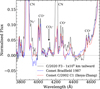 |
Fig. 16 Tailward spectrum of 20F3 overlaid with the spectra of comets Bradfield 1987 (Lutz et al. 1993) and Ikeya-Zhang (Cochran 2002), illustrating the detection of |

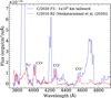 |
Fig. 17 Comparison of the tailward spectra of 20F3 and that of comet C/2016 R2 reported by Venkataramani et al. (2020). The two comets were not at all at the same distance from the Sun at the time of observation. This therefore merely illustrates the comparison with a comet that is well known to be rich in |

3.2.5 Higher abundance of  in 20F3
It is always challenging in low-resolution spectroscopy to fully resolve the  band, which lies near the strong CN emission band centred at 3880 Å. Although Cambianica et al. (2021) performed very high-resolution spectroscopy of 20F3, no ionic emission was reported, maybe because these high-resolution observations usually target the bright inner coma of the comet, whereas the ionic emission is detected primarily in the direction of the ion tail, where the emission of the neutral species has dropped strongly. In these cases, long-slit low-resolution spec-troscopy is advantageous because the spatial axis can be scanned to search for this emission.
In the absence of a high-resolution study to explore the possible higher abundance of  in 20F3, we directly compared the spectrum of comet C/2016 R2 (PanSTARRS) (Venkataramani et al. 2020), filled with ionic emission and without CN emission (Figure 17). By comparing the two comet spectra, we observe a similarity in the emission flux density for the CO+ (3-0) and (2-0) bands as well as for the 3915 Å peak of the
  emission. The drastic difference in the heliocentric distance of the two comets at the time of observation implies differences in the fluorescence efficiency, and hence, in the column densities. The
  band head in the two comets agrees well, which suggests the possibility of a higher
  flux density in 20F3 than what is measured from the visible band head.
To confirm the  ratio computed in Section 5, we incorporated modelling techniques similar to those used by Rousselot et al. (2022), but at lower resolution. The parameters used for this modelling are the heliocentric distance and velocity, and, because it is based on a Monte Carlo simulation, we used an evolutionary time of 10 000 s from an initial Boltzmann distribution, corresponding to a temperature of 80 K. We tried to model the
  emission band and the spectral region surrounding it using different models for the CN,
  , CO+, and C2 radicals. We used models similar to those described by Anderson et al. (2024), but convolved with a Gaussian instrument response function with a full width at half maximum (FWHM) that was adapted for the spectrum (i.e. 8 Å). For the C2 radical, we used a model similar to that described by Rousselot et al. (2012), calculated for the fluorescence equilibrium. Because the
  (0,0) emission bands near 3900 Å are blended with both CN and CO+ emission bands, it is unfortunately essential to model these emission bands as well as possible.
The overall spectral flux density of the CO+ emission bands can be estimated using the (3,0) (at 4000 and 4020 Å) and (2,0) (at 4252 and 4275 Å) emission bands (this last band is blended with the faint (5,2) emission band). In the latter band, it also blended with a fainter emission band of the  (0,1) emission band and C2 emission bands. A good fit of the (3,0) and (2,0) CO+ emission bands, including the
  (0,1) band, can be achieved with a ratio
  . With this ratio, which is probably the lowest possible value, the emission band
  (0,0) (the brightest) near the CN bright emission band cannot account for all the observed flux density at 3914 Å. An upper limit for the
  ratio can be estimated by fitting the flux density of the
  (0,0) band to the observation spectrum. In this case, we obtain
  . With this ratio, the fit of
  at 4275 Å appears to be overestimated compared to the observational spectrum. In this case, there are still a few unexplained emission lines near the
  emission bands, which are probably due to other species. These species probably cause part of the flux that is observed at 3914 Å.
Fig. 18 presents the different fits. Taking into account the findings and concluding that the ratio is the mean of the computed lower and upper limits, we report the  to be (4.8 ± 2.4) × 10–2. Similar to the interpretation provided by Opitom et al. (2019), since
  has been detected in comet 20F3 and the photodissociative ionisation of CO2 can also produce CO+, the N2/CO we computed should be considered as a lower limit.
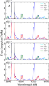 |
Fig. 18 Modelling of the |


4 Conclusions
We presented the long-slit low-resolution optical spectroscopic and photometric observation of the bright comet of 2020, C/2020 F3 (NEOWISE), using the 2m HCT and TRAPPIST-North telescope. The analysis of the spatial spectrum showed clear emission from the ionic species  , CO+,
  , and H2O+ in addition to the regular CN, C2, C3, NH2, and [OI] emission. Using these observational results, we conclude the following:
The computed production rate ratios, despite showing variations across the observation, classify the comet as gas rich with a typical carbon-chain composition.
The water-production rate computed using the spectral flux density of the forbidden oxygen line [OI] at 6300 Å agrees with the ratios reported by space- and ground-based measurements. These values may be regarded as reliable upper limits on the water-production rates.
The average nucleus rotation period was found to be 7.28 ± 0.79 hours from the observation of the CN jets, and the gas velocity was found to be 2.40 ± 0.25 km/s.
The average N2/CO for this comet, computed from the spectral observation, was found to be (3.0 ± 1.0) × 10–2, which agrees within the measurement errors, from ~40 000 km to ~100 000 km from the photocentre.
Taking into account the similarity of flux density for CO+ and
 in 20F3 and C/2016 R2, we used fluorescence modelling techniques to refine the ratio. With this, we estimated the N2/CO to be (4.8 ± 2.4) × 10–2. This ratio is considered as a lower limit to account for the detection of
  in the comet.
In addition to the usual ionic emission of
 , CO+ and H2O+, we identified emission at 4130 Å, corresponding to
  . Hence, 20F3 joins the list of great comets with identified
  emission and shows that this species can be detected from low-resolution spectra.
The
 ratio was computed to be 1.34 ± 0.21. Further modelling efforts are necessary to directly link the observed ratio with the known CO2/CO ratio of other comets.
The high
 ratio of 1.34 observed in C/2020 F3, combined with a relatively low
  ratio of 0.048, suggests that the comet probably formed in a region of the solar nebula in which the temperatures were cold enough for CO2 to condense efficiently, but too warm to trap significant N2. This is consistent with formation beyond the CO2 ice line (~70 K), but not far enough to retain more volatile species such as N2, and it indicates a likely origin in the moderately cold mid-to-outer nebula (~50–70 K). It is important to extend this type of analysis to other comets to refine our interpretation of the results.
Acknowledgements
We thank the staff of the Indian Astronomical Observatory, Hanle and Centre For Research & Education in Science & Technology, Hoskote, that made these observations possible. The facilities at IAO and CREST are operated by the Indian Institute of Astrophysics, Bangalore. Work at Physical Research Laboratory is supported by the Department of Space, Govt. of India. This publication makes use of data products from the TRAPPIST project, under the scientific direction of Prof. Emmanuel Jehin, Director of Research at the Belgian National Fund for Scientific Research (F.R.S.-FNRS). M.V.D is supported by the FNRS (Fond National pour la Recherche Scientifique; Belgium) through its FRIA PhD grant. TRAPPIST is funded by F.R.S.-FNRS under grant PDR T.0120.21, and TRAPPIST-North is funded by the University of Liège in collaboration with Cadi Ayyad University of Marrakech. The authors thank NASA, D. Schleicher, and the Lowell Observatory for the loan of a set of HB comet filters. A.K. acknowledges support from the Wallonia-Brussels International (WBI) grant. This work is a result of the bilateral Belgo-Indian projects on Precision Astronomical Spectroscopy for Stellar and Solar System bodies, BIPASS, funded by the Belgian Federal Science Policy Office (BELSPO, Govt. of Belgium; BL/33/IN22_BIPASS) and the International Division, Department of Science and Technology (DST, Govt. of India; DST/INT/BELG/P-01/2021 (G)).
References
- A’Hearn, M. F., Schleicher, D. G., Millis, R. L., Feldman, P. D., & Thompson, D. T. 1984, AJ, 89, 579 [Google Scholar]
- A’Hearn, M. F., Millis, R. C., Schleicher, D. O., Osip, D. J., & Birch, P. V. 1995, Icarus, 118, 223 [Google Scholar]
- Anderson, S. E., Rousselot, P., Jehin, E., et al. 2024, A&A, 692, A1 [NASA ADS] [CrossRef] [EDP Sciences] [Google Scholar]
- Anderson, S. E., Rousselot, P., Noyelles, B., Jehin, E., & Mousis, O. 2023, MNRAS, 524, 5182 [NASA ADS] [CrossRef] [Google Scholar]
- Aravind, K., Ganesh, S., Venkataramani, K., et al. 2021, MNRAS, 502, 3491 [Google Scholar]
- Aravind, K., Halder, P., Ganesh, S., et al. 2022, Icarus, 383, 115042 [NASA ADS] [CrossRef] [Google Scholar]
- Biermann, L., Giguere, P. T., & Huebner, W. F. 1982, A&A, 108, 221 [Google Scholar]
- Biver, N., Bockelée-Morvan, D., Paubert, G., et al. 2018, A&A, 619, A127 [NASA ADS] [CrossRef] [EDP Sciences] [Google Scholar]
- Bodewits, D., Országh, J., Noonan, J., Durian, M., & Matejcík, Š. 2019, ApJ, 885, 167 [Google Scholar]
- Bradley, L., Sipocz, B., Robitaille, T., et al. 2016, Astrophysics Source Code Library [record ascl:1609.011] [Google Scholar]
- Cambianica, P., Cremonese, G., Munaretto, G., et al. 2021, A&A, 656, A160 [NASA ADS] [CrossRef] [EDP Sciences] [Google Scholar]
- Cochran, A. L. 1985, AJ, 90, 2609 [Google Scholar]
- Cochran, A. L. 2002, ApJ, 576, L165 [Google Scholar]
- Cochran, A. L., & McKay, A. J. 2018, ApJ, 854, L10 [Google Scholar]
- Cochran, A. L., Cochran, W. D., & Barker, E. S. 2000, Icarus, 146, 583 [NASA ADS] [CrossRef] [Google Scholar]
- Cochran, A. L., Barker, E. S., & Gray, C. L. 2012, Icarus, 218, 144 [Google Scholar]
- Cochran, A. L., Nelson, T., McKay, A. J., et al. 2020, AAS/Div. Planet. Sci. Meeting Abstracts, 52, 111.03 [Google Scholar]
- Combi, M. R., Mäkinen, T., Bertaux, J. L., Quémerais, E., & Ferron, S. 2021, ApJ, 907, L38 [NASA ADS] [CrossRef] [Google Scholar]
- Dello Russo, N., Vervack, R. J., Kawakita, H., et al. 2016, Icarus, 266, 152 [Google Scholar]
- Drahus, M., Guzik, P., Stephens, A., et al. 2020, ATel, 13945, 1 [Google Scholar]
- Faggi, S., Lippi, M., Camarca, M., et al. 2021, AJ, 162, 178 [NASA ADS] [CrossRef] [Google Scholar]
- Farnham, T. L., Schleicher, D. G., & A’Hearn, M. F. 2000, Icarus, 147, 180 [Google Scholar]
- Fegley, Bruce, J., & Prinn, R. G. 1989, in The Formation and Evolution of Planetary Systems, eds. H. A. Weaver, & L. Danly (Massachusetts: Massachusetts Institute of Technology), 171 [Google Scholar]
- Feldman, P. D., A’Hearn, M. F., Festou, M. C., et al. 1986, Nature, 324, 433 [Google Scholar]
- Feldman, P. D., Festou, M. C., Tozzi, P., & Weaver, H. A. 1997, ApJ, 475, 829 [Google Scholar]
- Feldman, P. D., Cochran, A. L., & Combi, M. R. 2004, in Comets II, eds. M. C. Festou, H. U. Keller, & H. A. Weaver (Tucson: UA Press), 425 [Google Scholar]
- Festou, M. C., Feldman, P. D., & Weaver, H. A. 1982, ApJ, 256, 331 [Google Scholar]
- Fink, U. 2009, Icarus, 201, 311 [Google Scholar]
- Fink, U., & Combi, M. R. 2004, Planet. Space Sci., 52, 573 [Google Scholar]
- Fink, U., & Hicks, M. D. 1996, ApJ, 459, 729 [Google Scholar]
- Fink, U., Combi, M. R., & Disanti, M. A. 1991, ApJ, 383, 356 [Google Scholar]
- Hardy, P., Jehin, E., Rousselot, P., Hutsemékers, D., & Manfroid, J. 2023, LPI Contrib., 2851, 2148 [Google Scholar]
- Harrington Pinto, O., Womack, M., Fernandez, Y., & Bauer, J. 2022, PSJ, 3, 247 [Google Scholar]
- Haser, L. 1957, Bulletin de la Societe Royale des Sciences de Liege, 43, 740 [NASA ADS] [Google Scholar]
- Haser, L., Oset, S., & Bodewits, D. 2020, PSJ, 1, 83 [Google Scholar]
- Huebner, W. F., & Giguere, P. T. 1980, ApJ, 238, 753 [Google Scholar]
- Ivanova, O., Rosenbush, V., Luk’yanyk, I., et al. 2021, A&A, 651, A29 [NASA ADS] [CrossRef] [EDP Sciences] [Google Scholar]
- Jehin, E., Gillon, M., Queloz, D., et al. 2011, The Messenger, 145, 2 [NASA ADS] [Google Scholar]
- Jockers, K., Rosenbauer, H., Geyer, E. H., & Haenel, A. 1987, A&A, 187, 256 [Google Scholar]
- Kawakita, H., & Watanabe, J.-i. 2002, ApJ, 574, L183 [Google Scholar]
- Kim, S. J. 1999, Earth Planets Space, 51, 139 [Google Scholar]
- Korsun, P. P., Ivanova, O. V., & Afanasiev, V. L. 2006, A&A, 459, 977 [NASA ADS] [CrossRef] [EDP Sciences] [Google Scholar]
- Krishnakumar, A., Angchuk, D., Venkataramani, K., et al. 2020, ATel, 13897, 1 [Google Scholar]
- Langland-Shula, L. E., & Smith, G. H. 2011, Icarus, 213, 280 [CrossRef] [Google Scholar]
- Lew, H. 1976, Canadian J. Phys., 54, 2028 [Google Scholar]
- Lin, Z.-Y., Wang, C., Ip, W.-H., et al. 2020, ATel, 13886, 1 [NASA ADS] [Google Scholar]
- Lodders, K., Palme, H., & Gail, H. P. 2009, Landolt Börnstein, 4B, 712 [Google Scholar]
- Lutz, B. L., Womack, M., & Wagner, R. M. 1993, ApJ, 407, 402 [NASA ADS] [CrossRef] [Google Scholar]
- Mainzer, A., Bauer, J., Cutri, R. M., et al. 2014, ApJ, 792, 30 [Google Scholar]
- Manzini, F., Oldani, V., Ochner, P., et al. 2021, MNRAS, 506, 6195 [CrossRef] [Google Scholar]
- Marcus, J. N. 2007, International Comet Quarterly, 29, 39 [NASA ADS] [Google Scholar]
- McKay, A. J., Chanover, N. J., Morgenthaler, J. P., et al. 2012, Icarus, 220, 277 [Google Scholar]
- McKay, A. J., Cochran, A. L., Dello Russo, N., & DiSanti, M. A. 2020, ApJ, 889, L10 [Google Scholar]
- Mommert, M., Kelley, M. S. P., de Val-Borro, M., et al. 2019, Astrophysics Source Code Library [record ascl:1907.014] [Google Scholar]
- Morgenthaler, J. P., Harris, W. M., Scherb, F., et al. 2001, ApJ, 563, 451 [NASA ADS] [CrossRef] [Google Scholar]
- Morgenthaler, J. P., Harris, W. M., & Combi, M. R. 2007, ApJ, 657, 1162 [Google Scholar]
- Moulane, Y., Jehin, E., Opitom, C., et al. 2018, A&A, 619, A156 [NASA ADS] [CrossRef] [EDP Sciences] [Google Scholar]
- Moulane, Y., Jehin, E., Manfroid, J., et al. 2023, A&A, 670, A159 [NASA ADS] [CrossRef] [EDP Sciences] [Google Scholar]
- Mrozowski, S. 1947a, Phys. Rev., 72, 682 [Google Scholar]
- Mrozowski, S. 1947b, Phys. Rev., 72, 691 [Google Scholar]
- Opitom, C., Jehin, E., Manfroid, J., et al. 2015, A&A, 574, A38 [NASA ADS] [CrossRef] [EDP Sciences] [Google Scholar]
- Opitom, C., Hutsemékers, D., Jehin, E., et al. 2019, A&A, 624, A64 [NASA ADS] [CrossRef] [EDP Sciences] [Google Scholar]
- Opitom, C., Guilbert-Lepoutre, A., Besse, S., Yang, B., & Snodgrass, C. 2020, A&A, 644, A143 [NASA ADS] [CrossRef] [EDP Sciences] [Google Scholar]
- Owen, T., & Bar-Nun, A. 1995, Icarus, 116, 215 [NASA ADS] [CrossRef] [Google Scholar]
- Rousselot, P., Jehin, E., Manfroid, J., & Hutsemékers, D. 2012, A&A, 545, A24 [NASA ADS] [CrossRef] [EDP Sciences] [Google Scholar]
- Rousselot, P., Anderson, S. E., Alijah, A., et al. 2022, A&A, 661, A131 [NASA ADS] [CrossRef] [EDP Sciences] [Google Scholar]
- Rousselot, P., Jehin, E., Hutsemékers, D., et al. 2024, A&A, 683, A50 [NASA ADS] [CrossRef] [EDP Sciences] [Google Scholar]
- Rubin, M., Altwegg, K., Balsiger, H., et al. 2015, Science, 348, 232 [NASA ADS] [CrossRef] [Google Scholar]
- Schleicher, D. G. 2010, AJ, 140, 973 [Google Scholar]
- Schleicher, D. G., Millis, R. L., & Birch, P. V. 1998, Icarus, 132, 397 [NASA ADS] [CrossRef] [Google Scholar]
- Schultz, D., Li, G. S. H., Scherb, F., & Roesler, F. L. 1992, Icarus, 96, 190 [Google Scholar]
- Sekanina, Z., & Larson, S. M. 1984, AJ, 89, 1408 [Google Scholar]
- Smyth, H. D. 1931, Phys. Rev., 38, 2000 [Google Scholar]
- Tseng, W. L., Bockelée-Morvan, D., Crovisier, J., Colom, P., & Ip, W. H. 2007, A&A, 467, 729 [NASA ADS] [CrossRef] [EDP Sciences] [Google Scholar]
- Umbach, R., Jockers, K., & Geyer, E. H. 1998, A&AS, 127, 479 [NASA ADS] [CrossRef] [EDP Sciences] [Google Scholar]
- Venkataramani, K., Ganesh, S., & Baliyan, K. S. 2020, MNRAS, 495, 3559 [NASA ADS] [CrossRef] [Google Scholar]
- Villanueva, G. L., Liuzzi, G., Faggi, S., et al. 2022, Fundamentals of the Planetary Spectrum Generator (USA: Library of Congress) [Google Scholar]
- Villanueva, G. L., Smith, M. D., Protopapa, S., Faggi, S., & Mandell, A. M. 2018, J. Quant. Spec. Radiat. Transf., 217, 86 [NASA ADS] [CrossRef] [Google Scholar]
- Weaver, H. A., Feldman, P. D., McPhate, J. B., et al. 1993, LPI Contrib., 810, 309 [Google Scholar]
- Wyckoff, S., & Wehinger, P. A. 1976, ApJ, 204, 604 [Google Scholar]
- Wyckoff, S., Heyd, R. S., & Fox, R. 1999, ApJ, 512, L73 [Google Scholar]
- Wyckoff, S., Wehinger, P. A., Spinrad, H., & Belton, M. J. S. 1986, ESA SP, 250, 311 [Google Scholar]
- Ye, Q., Zhang, Q., Brewer, J., Knight, M., & Kelley, M. 2020, AAS/Div. Planet. Sci. Meeting Abstracts, 52, 111.02 [Google Scholar]
Panoramic Survey Telescope and Rapid Response System.
TRAnsiting Planets and PlanetesImals Small Telescope.
Solar Wind ANisotropies.
Solar and Heliospheric Observatory.
All Tables
Production rates and rate ratios for the main neutral molecules in 20F3 observed on 24 luly 2020.
All Figures
|
Fig. 1 Orientation of the slit overlaid on an HFOSC image at the time of acquisition on 24 July 2020. |
| In the text | |
|
Fig. 2 Panel a: 2D spectrum of 20F3. The blue wavelength starts from the top. The white arrows denote the visually noted doublets in the anti-sunward direction. Panel b: various apertures (horizontal bars) for the spectral extraction compared to the comet photon density profile around the nucleus. Ε and W represent the apertures used in the east and west directions, respectively. |
| In the text | |
|
Fig. 3 Long-slit spectra of 20F3 observed on 24 July 2020, extracted at photocentre (top panel) and at the extreme regions of the slits in the tailward and anti-tailward directions (bottom panel). The arrows depict the dissimilarity regions for spectra extracted from extreme regions of the slit. |
| In the text | |
|
Fig. 4 Median column density profiles of the main molecules detected in the spectrum. |
| In the text | |
|
Fig. 5 Detected emission for spectra extracted (a) and (b) at photocentre, and (c) and (d) 105 km in the tailward direction. |
| In the text | |
|
Fig. 6 Rectangular slit for which the Haser factor computation was performed from a 2D image of the column density from the Haser model. |
| In the text | |
|
Fig. 7 Logarithmic production rates of OH, NH, CN, C3, and C2 detected in 20F3 as a function of time and heliocentric distance. The vertical dashed line indicates the perihelion on 3 July 2020, at 0.29 au. The red mark in each symbol represents the corresponding measurements from the spectroscopic observation. |
| In the text | |
|
Fig. 8 A(0)fρ parameter of 20F3 at 10 000 km from the broad- and narrow-band filters as a function of time and heliocentric distance. |
| In the text | |
|
Fig. 9 Optical light curve of 20F3 measured within a 5-arcsecond aperture as a function of time and distance to perihelion. The vertical dashed line indicates the perihelion at 0.29 au on 3 July 2020. |
| In the text | |
|
Fig. 10 Logarithm of the production rates and dust-to-gas ratios of C/2020 F3 with respect to CN and to OH as a function of time and heliocentric distance. The horizontal dashed blue line and the shaded region represent the mean ratios and range of ratios for comets with typical carbon composition as defined by A’Hearn et al. (1995). The red mark in a few panels represents the corresponding measurements from the spectroscopic observation. The error bars correspond to the 1σ absolute errors. |
| In the text | |
|
Fig. 11 Azimedian (left) and rotational (right) CN narrow-band filtered images selected the night starting 22 July, one hour apart. The images are oriented with north up and east to the left. The red spirals follow the northern jet, which was used for the rotational and velocity analysis. |
| In the text | |
|
Fig. 12 Comparison of Haser model fittings for the observed (O) column densities of CN, C2, and C3 making use of respective scale-lengths defined by A’Hearn et al. (1995) (A), Langland-Shula & Smith (2011) (B), and Cochran et al. (2012) (C). |
| In the text | |
|
Fig. 13 6335 Å NH2 peak used to decontaminate the NH2 contribution in the [OI] 6300 Å line. |
| In the text | |
|
Fig. 14 Comparison of water production of 20F3 computed in this work using the 6300 Å [OI] line spectral flux density (S) and OH narrow-band images (P) with those reported by Combi et al. (2021) and Faggi et al. (2021). The error bars correspond to 1σ absolute errors. |
| In the text | |
|
Fig. 15 Spectrum of 20F3 extracted from the tailward direction, 1 × 10⁵ km away from the photocentre (a) depicting the detection of ionic emission and a few unidentified emissions; (b) overplotted with the modelled spectrum of CO+ (Rousselot et al. 2024) convolved with the instrument profile, and (c) overplotted with the laboratory spectra of H2O+ (Lew 1976) convolved with the instrument profile. |
| In the text | |
|
Fig. 16 Tailward spectrum of 20F3 overlaid with the spectra of comets Bradfield 1987 (Lutz et al. 1993) and Ikeya-Zhang (Cochran 2002), illustrating the detection of |
| In the text | |
|
Fig. 17 Comparison of the tailward spectra of 20F3 and that of comet C/2016 R2 reported by Venkataramani et al. (2020). The two comets were not at all at the same distance from the Sun at the time of observation. This therefore merely illustrates the comparison with a comet that is well known to be rich in |
| In the text | |
|
Fig. 18 Modelling of the |
| In the text | |
Current usage metrics show cumulative count of Article Views (full-text article views including HTML views, PDF and ePub downloads, according to the available data) and Abstracts Views on Vision4Press platform.
Data correspond to usage on the plateform after 2015. The current usage metrics is available 48-96 hours after online publication and is updated daily on week days.
Initial download of the metrics may take a while.