| Issue |
A&A
Volume 701, September 2025
|
|
|---|---|---|
| Article Number | A41 | |
| Number of page(s) | 20 | |
| Section | Astrophysical processes | |
| DOI | https://doi.org/10.1051/0004-6361/202554936 | |
| Published online | 02 September 2025 | |
Millimeter emission from supermassive black hole coronae
1
Department of Space, Earth and Environment, Chalmers University of Technology, SE-412 96 Gothenburg, Sweden
2
Department of Space, Earth and Environment, Chalmers University of Technology, Onsala Space Observatory, 43992 Onsala, Sweden
3
Instituto de Estudios Astrofísicos, Facultad de Ingeniería y Ciencias, Universidad Diego Portales, Santiago, 8370191
Chile
4
Kavli Institute for Astronomy and Astrophysics, Peking University, Beijing, 100871
China
5
Theoretical Physics IV: Plasma-Astroparticle Physics, Faculty for Physics & Astronomy, Ruhr University Bochum, 44780 Bochum, Germany
6
Ruhr Astroparticle And Plasma Physics Center (RAPP Center), Ruhr-Universität Bochum, 44780 Bochum, Germany
7
National Radio Astronomy Observatory, 520 Edgemont Road, Charlottesville, VA, 22903
USA
8
National Astronomical Observatory of Japan, 2-21-1, Osawa, Mitaka, Tokyo, 181-8588
Japan
9
Observatorio Astronómico Nacional (OAN-IGN)-Observatorio de Madrid, Alfonso XII, 3, 28014 Madrid, Spain
10
Observatoire de Paris, LUX, Collège de France, CNRS, PSL University, Sorbonne University, 75014 Paris, France
11
Steward Observatory, University of Arizona, 933 N Cherry Avenue, Tucson, AZ, 85721
USA
12
Jodrell Bank Centre for Astrophysics, The University of Manchester, M13 9PL, UK
13
Leiden Observatory, Leiden University, PO Box 9513 2300 RA Leiden, The Netherlands
14
George P. and Cynthia Woods Mitchell Institute for Fundamental Physics and Astronomy, Texas A&M University, College Station, TX, 77845
USA
15
CSIRO Space and Astronomy, ATNF, PO Box 1130 Bentley, WA, 6102
Australia
16
Institute of Astronomy, The University of Tokyo, 2-21-1, Osawa, Mitaka, Tokyo, 181-0015
Japan
17
National Radio Astronomy Observatory, 520 Edgemont Road, Charlottesville, VA, 22903
USA
18
Department of Astronomy, University of Virginia, 530 McCormick Road, Charlottesville, VA, 22903
USA
19
Centro de Astrobiología (CAB), CSIC-INTA, Camino Bajo del Castillo s/n, E-28692 Villanueva de la Cañada, Madrid, Spain
20
National Astronomical Observatory of Japan, 2-21-1 Osawa, Mitaka, Tokyo, 181-8588
Japan
21
Max-Planck-Institut für Radioastronomie, Auf dem Hügel 69, D-53121 Bonn, Germany
22
Xinjiang Astronomical Observatory, Chinese Academy of Sciences, 830011 Urumqi, PR China
23
Instituto de Física Fundamental, CSIC, Calle Serrano 123, E-28006 Madrid, Spain
24
European Southern Observatory, Alonso de Córdova, 3107, Vitacura, Santiago, 763-0355
Chile
25
Joint ALMA Observatory, Alonso de Córdova, 3107, Vitacura, Santiago, 763-0355
Chile
26
Instituto de Física Fundamental, CSIC, Calle Serrano 123, 28006 Madrid, Spain
27
Center for Interdisciplinary Exploration and Research in Astrophysics (CIERA) Northwestern University, Evanston, IL, 60208
USA
⋆ Corresponding author: This email address is being protected from spambots. You need JavaScript enabled to view it.
Received:
1
April
2025
Accepted:
26
June
2025
Abstract
Context. Active galactic nuclei (AGNs) host accreting supermassive black holes (SMBHs). The accretion process can lead to the formation of a hot, X-ray emitting corona close to the SMBH that can accelerate relativistic electrons. Observations in the millimeter band can probe its synchrotron emission.
Aims. We intend to provide a framework to derive physical information of SMBH coronae by modelling their spectral energy distribution (SED) from radio to far-infrared frequencies. We also explore the possibilities of deriving additional information from millimeter observations, such as the SMBH mass, and studying high-redshift lensed sources.
Methods. We introduce a corona emission model based on a one-zone spherical region with a hybrid thermal and non-thermal plasma. We investigated the dependence of the corona SED on different parameters such as size, opacity, and magnetic field strength. Other galactic emission components from dust, ionised gas, and diffuse relativistic electrons were also included in the SED fitting scheme. We applied our code consistently to a sample of radio-quiet AGNs with strong indications of a coronal component in the millimeter.
Results. The detected millimeter emission from SMBH coronae is consistent with a non-thermal relativistic particle population with an energy density that is ≈0.5–10% of that in the thermal plasma. This requires magnetic energy densities close to equipartition with the thermal gas and corona sizes of 60–250 gravitational radii. The model can also reproduce the observed correlation between millimeter emission and SMBH mass when we accounted for the uncertainties in the corona size.
Conclusions. The millimeter band offers a unique window into the physics of SMBH coronae, enabling the study of highly dust-obscured sources and high-redshift lensed quasars. Gaining a deeper understanding of the relativistic particle population in SMBH coronae can provide key insights into their potential multiwavelength and neutrino emission.
Key words: radiation mechanisms: non-thermal / galaxies: nuclei / radio continuum: galaxies / submillimeter: galaxies
© The Authors 2025
 Open Access article, published by EDP Sciences, under the terms of the Creative Commons Attribution License (https://creativecommons.org/licenses/by/4.0), which permits unrestricted use, distribution, and reproduction in any medium, provided the original work is properly cited.
This article is published in open access under the Subscribe to Open model. This email address is being protected from spambots. You need JavaScript enabled to view it. to support open access publication.
1. Introduction
An active galactic nucleus (AGN) is produced when a supermassive black hole (SMBH) accretes matter from its surrounding medium. The material around an SMBH is pulled inward by the strong gravitational field and spirals, forming an accretion disc. Processes related to turbulent magnetic viscosity in the accretion disc cause the material to lose angular momentum and fall towards the SMBH, releasing huge amounts of gravitational energy. The material then heats up and radiates across a broad range of wavelengths (e.g. Balbus & Hawley 1998). The accretion process is very efficient in converting gravitational potential energy into other forms, such as radiation, magnetic fields, and particle acceleration. Moreover, close to the innermost regions of the accretion disc, magnetic reconnection events can heat the gas to extremely high temperatures (∼109 K), giving rise to a compact, hot region known as the corona (e.g. Haardt & Maraschi 1991; Kamraj et al. 2022).
Most (∼90%) AGNs emit only weakly at radio wavelengths and are therefore classified as radio quiet (RQ). Although these AGNs lack a powerful radio jet (Urry & Padovani 1995), radio emission at 22 GHz is commonly detected (Smith et al. 2020; Magno et al. 2025). Interestingly, millimeter (mm) emission is also frequently observed in nearby RQ AGNs, with most of the mm continuum flux originating from an unresolved core. Several studies have argued that this radiation is synchrotron emission produced in the corona, which also produces the hard X-ray emission above 2 keV through inverse-Compton scattering of thermal disc photons, ubiquitously observed in AGNs (e.g. Laor & Behar 2008; Inoue & Doi 2014; Behar et al. 2018; Panessa et al. 2019). Recent studies strongly support this interpretation: High-resolution (∼0.1–1″) ALMA observations of nearby AGNs revealed a tight correlation between X-ray emission and mm continuum at ∼200 GHz (Kawamuro et al. 2022) and at ∼100 GHz (Ricci et al. 2023), as well as a correlation between the SMBH mass and the mm flux density at ∼230 GHz (Ruffa et al. 2024). In addition, correlated variability of X-ray and mm emission on year-timescales was found in NGC 1566 Jana et al. (2025). Together, these results support the idea that the corona plays a key role in the mm emission from RQ AGNs.
The X-ray corona is expected to be very compact, rc = Rc/Rg ∼ 10–50, where Rg = GMBH/c2 is the gravitational radius, and MBH is the mass of the SMBH (e.g. Fabian et al. 2015; Inoue & Doi 2018). Nonetheless, the size of the corona is a topic of debate, with spectrotiming analysis of X-ray emission in Galactic X-ray binaries (XRBs) favouring dynamical coronae that vary in size from tens to hundreds of Rg (e.g. Karpouzas et al. 2021). Even the geometry of the corona (lamp post, toroidal, spherical, or sandwich-like) is unknown (e.g. Bambi et al. 2021, and references therein). Models for dynamical, outflowing coronae with sizes rc ∼ 10–1000 have also been suggested in the context of XRBs (Kylafis et al. 2023); this is remarkably consistent with the results of mm variability in the RQ AGN IC 4329A (Shablovinskaya et al. 2024). On the topic of variability, we also highlight the results by Petrucci et al. (2023), who reported rapid variability in mm and X-ray emission from MCG+08−11−11 within a day, and by Michiyama et al. (2024), who revealed mm variability in a few days in GRS 1734−292. The fast variability strongly supports the hypothesis that the mm emission comes from a compact region with rc ∼ 20–400. Altogether, this shows that the size of the corona remains a topic of debate.
In addition, the presence of ultra-relativistic particles in coronae is supported by both theoretical and observational evidence. Magnetic reconnection events, as well as other processes related to internal shocks and/or turbulence, might accelerate relativistic particles out of thermal equilibrium (non-thermal particles; e.g. Inoue et al. 2008; Beloborodov 2017; Sironi & Beloborodov 2020; Grošelj et al. 2024; Nättilä 2024). In the case of a corona, the presence of extremely hot gas (kT > 100 keV) leads to the co-existence of thermal and non-thermal relativistic particles (e.g. Özel et al. 2000), which we refer to as a hybrid plasma. Another independent proof of a non-thermal electron population in the corona is the hard X-ray or soft gamma-ray tail detected in the XRBs Cyg X-1 (Zdziarski et al. 2021) and MAXI J1820+070 (Cangemi et al. 2021). A scenario involving (hadronic) cosmic rays in the corona is also compatible with the MeV polarised emission detected in Cyg X-1 (Romero et al. 2014), and possibly with its sub-GeV and TeV emission (Fang et al. 2024). In addition, γ-ray emission in the 1–300 GeV energy range was detected in the stacked signal of 37 RQ AGNs, which was interpreted to be produced in extended coronae (The Fermi-LAT Collaboration 2020). Furthermore, several studies have suggested that significant neutrino emission can be produced by cosmic rays in SMBH coronae (e.g. Inoue et al. 2019; Murase et al. 2020; Kun et al. 2024; Fang et al. 2024), consistent with the neutrino emission from NGC 1068 (Inoue et al. 2020; Eichmann et al. 2022). This scenario is particularly attractive because it can account for gamma-ray luminosity that is orders of magnitude lower than the neutrino luminosity, as the corona environment produces strong gamma-gamma absorption.
A relatively new window for studying SMBH corona is in the mm atmospheric bands. The relativistic electrons in the corona interact with the local magnetic fields and emit synchrotron radiation with a spectral energy distribution (SED) that peaks at around 100–300 GHz, depending on the plasma conditions in the corona and its non-thermal particle content (Inoue & Doi 2014; Inoue et al. 2019). Although corona properties such as temperature and optical depth can be derived from X-ray observations (e.g. Fabian et al. 2015; Ricci et al. 2018), the magnetic field strength and non-thermal particle population content can only be inferred by modelling the mm emission (e.g. Inoue & Doi 2018).
We present a framework for modelling the SEDs of RQ AGNs. We pay special attention to the synchrotron emission from AGN coronae and its dependence on different physical parameters. We then apply this model consistently to a sample of objects for which good spectral coverage is available in order to derive the most relevant parameters of the coronae.
2. Emission model
The nuclear region of an RQ galaxy (inner ∼100 pc) can contain large reservoirs of ionised gas, dust, cosmic rays, and an AGN. Thus, the observed continuum radio-to-submm SED of an RQ galaxy is the combination of several contributions, each with a distinct shape. We assumed that these components are independent of each other and that the total emission is simply the sum of all components. The most relevant SED components that we consider are listed below1
-
Ionised gas: The warm, ionised gas in the galaxy emits free–free (f–f) radiation that can be relevant at frequencies between ∼10–100 GHz, where it presents a spectral index α = −0.1 (e.g. Murphy et al. 2018). The intensity of this emission is expected to scale with the amount of ionised gas, and thus, with the star formation rate (SFR; Murphy et al. 2011). In the simplest case, this emission can be parametrised as
 (1)
(1)where Aff is a normalisation constant and ν0 is a reference frequency (fixed at 100 GHz). We note that at low frequencies, this emission can actually drop as the medium becomes optically thick (α = 2 instead of −0.1). The turnover frequency depends most strongly on the density of the medium, but also on its structure (e.g. Ramírez-Olivencia et al. 2022)
-
A diffuse cosmic-ray electron population: Its origin is likely related to the SFR, where supernova remnants and winds from massive stars accelerate cosmic rays that diffuse in the galaxy (e.g. Lacki & Thompson 2010; Kornecki et al. 2022) or to extended jets (Urry & Padovani 1995). This component produces optically thin synchrotron emission with a steep spectral index between −0.5 and −1 (e.g. Heesen et al. 2022; An et al. 2024), which dominates at low frequencies in the radio-cm range (≲10 GHz). In the simplest case, this emission can be parametrised as
 (2)
(2)where Asy is a normalisation constant, ν0 is a reference frequency (fixed at 100 GHz), and αsy is the intrinsic spectral index of the synchrotron emission. At low frequencies, the behaviour of this component can deviate from a simple power law, most likely due to f–f absorption in the ionised gas that flattens the spectrum at lower frequencies (e.g. Kornecki et al. 2022; Dey et al. 2024), consistent with what is observed in studies at ν < 1 GHz of a large sample of galaxies (Heesen et al. 2022; An et al. 2024). If the ionised medium is inhomogeneous and clumpy, the absorption depends on the opacity and distribution of the clumps. This can result in significant absorption of the synchrotron emission, but part of it can also propagate between the clumps unaffectedly (e.g. Lacki 2013; Ramírez-Olivencia et al. 2022). We refrained from including these effects in our model because it would introduce additional free parameters that do not assist us in our main goal, which is to isolate and study the corona component that peaks at much higher frequencies.
-
Corona: The intrinsic synchrotron SED is a power law with a negative spectral index (α ∼ −0.5 to −1), but lower-frequency radiation is absorbed by the relativistic electrons via synchrotron self-absorption (SSA), producing a turnover in the SED that shifts to a positive spectral index α = 5/2 (e.g. Margalit & Quataert 2021). The position of the turnover frequency νSSA ≈ 100–300 GHz, depends on the plasma conditions in the corona, such as its density, size, and the magnetic field strength (see forthcoming Sect. 3.1). This results in an SED with a rather pronounced peak at ν ∼ νSSA. As the main goal of this work is to derive the physical properties of the corona, in this case, we did not adopt a simple phenomenological model, but instead computed the SED in a physically motivated way, as detailed in Sect. 2.1. We highlight that this region is extremely compact and can exhibit very high brightness temperatures (potentially up to ∼109 K if observed with a 10 μas resolution at 100 GHz, adopting as reference a flux density of ∼1 mJy).
-
Dust: Its continuum emission dominates the SED at high frequencies (≳300 GHz, depending on the source and the angular resolution of the observations). Within the Rayleigh-Jeans regime, this can be modelled as a modified black-body spectrum characterised by the frequency ντ1 at which the dust opacity becomes equal to unity, and the index β of the opacity coefficient κν ∝ νβ (with β ≈ 1–2). At ν < ντ1, the SED is optically thin and has a spectral index α = 2 + β, while at ν > ντ1, it is optically thick and α = 2. This is parametrised as
 (3)
(3)where Ad is a normalisation constant, ν0 is a reference frequency (fixed at 100 GHz), and τd = (ν/ντ1)β. We note that the dust mass is Md ∝ ντ1 (Draine 2011), so that an accurate determination of ντ1 can help us to estimate dust masses, although this would typically require a good spectral coverage between 400–1000 GHz that is challenging to obtain. We also note that at the frequencies at which the dust becomes optically thick, it could also absorb the emission from the corona. This would depend on geometrical assumptions regarding the dust distribution along the line of sight, however, and it would only affect the optically thin part of the corona SED, which is difficult to observe as it is expected to be faint and typically below the dust continuum emission. We thus neglected this effect in our model fitting. In addition, rapidly spinning dust grains can produce anomalous microwave emission (AME) that peaks around ν ∼ 30 GHz, although in certain conditions, it can reach ∼100 GHz (Dickinson et al. 2018; Murphy et al. 2020). This component is faint, however, and in extragalactic contexts, it has only been detected in off-nuclear star-forming regions in a handful of nearby galaxies (e.g. Poojon et al. 2024; Fernández-Torreiro et al. 2024). It is thus unlikely that this component is bright in the sources of our sample, which in fact do not present a bump in their SED at (rest-frame) frequencies of ∼30 GHz (Sect. 3). For this reason, we did not include an AME emission component in our model.
2.1. Corona emission
We developed a corona emission model based on the one-zone model presented by Inoue et al. (2019), in which the corona is a hybrid plasma with a thermal and a non-thermal particle population. We therefore used the numerical code from Margalit & Quataert (2021)2, which computes the synchrotron SED of a hybrid plasma. We modelled the corona as a spherical region of size Rc = rcRg, with Rg the gravitational radius and rc a dimensionless radius. The thermal plasma is characterised by its temperature Tc and number density nth, 0. The latter is parametrised through the Thomson opacity τT as nth, 0 = τT/(σTRc). The energy density in thermal electrons is Uth, e = a(Θ) Θ nth, 0 mec2, where is Θ = kTc/(mec2) is a dimensionless temperature, and a(Θ) = (6 + 15Θ)/(4 + 5Θ) (Margalit & Quataert 2021).
Following Margalit & Quataert (2021), for the non-thermal population, we defined a minimum Lorentz factor γmin(Θ) = 1 + a(Θ) Θ, such that at energies above Emin = γminmec2, the particle energy distribution is
 (4)
(4)
Here, p is the spectral index of the electron distribution without cooling, tdyn is the characteristic dynamical timescale, for which we adopted the free-fall time tdyn = Rc/vff (with  the free-fall velocity; Inoue et al. 2019), and tsy is the synchrotron cooling timescale. We highlight that the values of tsy and tdyn were calculated self-consistently in the model for any given set of parameters (MBH, rc, etc.).
The next step was to define the non-thermal electron population in the corona and the magnetic field. For this, additional free parameters had to be introduced. One sensible way to do this is to use the energy density in thermal electrons as a reference. We defined the ratio of the energy densities in the magnetic field and thermal electrons ϵB = UB/Uth, e, and the ratio of the energy density in non-thermal electrons and thermal electrons δ = Unt, e/Uth, e. To constrain the model further, we assumed δ < 1, as otherwise the non-thermal electrons would dominate in the corona, which does not seem to be the case (e.g. Zdziarski et al. 2021); we further note that Inoue & Doi (2018) fixed this parameter to 0.04. Another consideration was that magnetic fields are thought to play a major role in heating the corona and accelerating relativistic particles (e.g. Beloborodov 2017; Sironi & Beloborodov 2020), and therefore, it should be the case that ϵB is of order unity and ϵB > δ. We can thus impose an energy condition UB = ηUnt, where Unt is the total energy in non-thermal particles. This is commonly written as Unt = Unt, e + Unt, p = (1 + ξe, p) Unt, e, where ξe, p is the ratio of the energy density in relativistic protons and electrons. With these definitions, we rewrote ϵB = η δ (1 + ξe, p). Either because relativistic protons are easier to accelerate or because relativistic electrons cool faster than protons, the energy density in non-thermal protons is higher than that of electrons (e.g. Eichmann et al. 2022), and we therefore fixed ξe, p = 40 (roughly corresponding to  ; e.g. Merten et al. 2017). We additionally fixed η = 1, corresponding to an energy equipartition condition between non-thermal particles and magnetic fields. In this way, we removed a free parameter by the condition ϵB = 41 δ.
A related parameter that is commonly used to characterise the plasma conditions is the σ parameter, defined as σ = B2/(4πnth, emec2). Neglecting some factors of order unity, we approximated σ ≈ ϵB Θ, which helped us to understand the dependence of σ on the model parameters. In particular, for a highly magnetised plasma, we expect σ to be of the order of unity. Similarly, this can be compared with the plasma βB parameter, defined as the ratio of thermal and magnetic pressures, βB = Pth/PB, which can be rewritten as3βB ∼ 5/ϵB.
After we defined the thermal and non-thermal particle populations together with the physical properties of the corona, the code calculated the synchrotron SED, taking into account the emissivity and opacity (SSA) from both populations. In this way, the synchrotron SED (including νSSA) was self-consistently calculated for any set of parameters.
We finally converted the specific luminosities into flux densities in order to compare them with observed SEDs. To do this, we used the Planck18 library available in astropy to convert z into a luminosity distance and the rest-frame frequencies into the observed frame as νobs = ν/(1 + z). Finally, to study lensed sources (as explored in Sect. 3.2), we introduced a multiplicative amplification factor μ to the intrinsic luminosity.
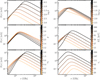 |
Fig. 1. Corona SEDs in which only one parameter was varied at a time, as indicated in the colour bar of each panel. The fiducial values are D = 100 Mpc, MBH = 108 M⊙, τT = 0.25, kTc = 166 keV, rc = 130, log ϵB = 0, log δ = −1.5, and p = 2.7. More details are discussed in Sect. 3.1. |
2.2. Parameter fitting
We developed a code4 that calculates the total SED from the physical coronal model, together with the phenomenological components described in Sect. 2. We used the Python package Bilby (Ashton et al. 2019) to fit the SED using the standard sampler for Markov chain Monte Carlo emcee (Foreman-Mackey et al. 2013). One key issue is dealing with observations with different angular resolutions. The corona is extremely compact, and its emission should therefore be point-like in all observations. The other galactic components are most likely extended and inhomogeneous, so that it is not possible to scale the observed flux density with the beam size in a reliable way. For this reason, we used beam-matched data whenever possible, even when this required compromising the angular resolution. The main drawback was that the corona emission is not very bright and can therefore be well below the continuum of other galactic components in observations with a poor angular resolution that collect too much diffuse emission, making it undetectable. For this reason, we filtered out observations with a coarse angular resolution (typically > 1″, corresponding to linear scales > 100 pc for galaxies at distances beyond 20 Mpc) and considered them only as strict upper limits (ULs) for the total flux density. Similarly, for observations with a significantly higher angular resolution than the rest of the dataset, for instance, from very large baseline interferometry (VLBI), we considered them only as strict lower limits (LLs) of the total flux density. In both cases, we left a 1σ margin to be more conservative about using points as strict ULs or LLs, that is, for a measured flux of Sν ± ΔSν, we chose SUL = Sν + ΔSν and SLL = Sν − ΔSν.
To reduce the number of free parameters in the model, we used the parametrisation for ϵB(δ) described in Sect. 2.1. In addition, when τT and Tc were not directly determined from X-ray data, we adopted the parametrisation for Tc(τT) from Tortosa et al. (2018). As a reference, this corresponds to kTc ≃ 166 keV for the most typical case of τT ≃ 0.25 (Ricci et al. 2018), while for τT ≃ 1, we obtained kTc ≃ 63 keV. We summarise all the model parameters and the range of values that they can take in Table 1. We note that for quantities that can span several orders of magnitude, we fit the logarithm of the quantity.
This code has been used to model the SEDs of IC 4329A (Shablovinskaya et al. 2024) and NGC 1068 (Mutie et al. 2025). As a sanity check, we verified that the sizes derived with this approach agree well with the simple analytical estimate from Eq. (4) in Shablovinskaya et al. (2024). Additionally, we confirmed that our results are consistent with those reported by Inoue & Doi (2018) when we fixed the same parameters as they did.
Throughout this work, the quoted error bars correspond to the 16th–84th percentile range (the 1σ confidence intervals for Gaussian distributions) and were derived from the posterior distribution. We also assumed a conservative flux uncertainty to account for systematic errors in absolute flux calibrations, such that the total error bar is  , with ΔSsta the statistical uncertainty and ΔSsys = fsys Sν the assumed systematic error. The factor fsys was fixed to 5% for all observations, except for ALMA observations at B6–8 (212–500 GHz) and B9–10 (600–900 GHz), for which it was 10% and 20%, respectively5.
3. Results
3.1. Parameter exploration
We explored the corona SED response to the different model parameters in order to gain some insight into the interpretation of the observed SEDs. To do this, we considered a reference case with the following parameters: D = 100 Mpc, MBH = 108 M⊙, τT = 0.25, kTc = 166 keV, rc = 140, ϵB = 1.0, δ = 0.01, and p = 2.7. First, we varied one parameter at a time. The results are shown in Fig. 1. Some highlights are listed below.
-
Higher δ values mean more relativistic electrons and therefore lead to a higher emission and a higher opacity. Below νSSA, the emission is optically thick, so that a larger number of non-thermal electrons does not increase the flux, which remains constant for all δ values. The value of νSSA increases with increasing δ.
-
The value of ϵB sets the magnetic field strength. Stronger magnetic fields lead to more SSA, and therefore, νSSA depends strongly on this parameter. Moreover, for very small magnetic fields (ϵB < 0.01), the electrons do not cool efficiently (tsy > tdyn), and the flux in the optically thin part of the SED varies significantly with ϵB. For values of ϵB > 0.01, the dependence of the SED with this parameter is rather weak, however.
-
The value of p mostly affects the slope in the optically thin part of the spectrum. Thus, observational restrictions on this parameter can only be obtained with observations at frequencies that are significantly higher than νSSA. The frequency νSSA itself does not vary significantly with p.
-
Increasing the corona temperature increases Uth, e and therefore also Unt, e and UB for fixed values of δ and ϵB. Thus, increasing Tc has a similar impact as increasing δ and ϵB. The main difference occurs for kTc ∼ 300 keV, at which point the thermal electrons play a significant role in further absorbing the emission below νSSA, although their emission is negligible (we refer to Margalit & Quataert 2021, for a scenario in which the thermal electrons can have an even more dominant role). For completeness, we explore the emission from thermal electrons in more detail in Appendix A.
-
The Thomson opacity defines the density of thermal particles, and it therefore impacts Uth, e. The increase in τT therefore has a similar impact as the increase in kTc.
-
For a fixed MBH, the value of rc determines the size of the corona. A larger corona produces more emission, and it is also more transparent as it is more diluted (as nth, 0 ∝ τT rc−1). Thus, νSSA decreases with an increasing rc. For this parameter alone, an increase in the total peak flux is accompanied by a decrease in νSSA, and it is therefore a key parameter in the SED fitting to obtain the correct peak position and flux.
As discussed in Sect. 2.1, we reduced the number of free parameters by assuming an energy condition of the form ϵB = η δ (1 + ξe, p) = 41 δ and the observational relation for Tc(τT) from Tortosa et al. (2018). The results are shown in Fig. 2. We summarise them below.
-
Increasing δ (with ϵB(δ)) leads to a significant increase in both νSSA and the peak flux.
-
Changes in τT (with Tc(τT)) have negligible effects in the SED because the SED depends in similar ways on τT and Tc, and τT and Tc are anti-correlated and therefore compensate for the changes in the SED. This means that, in general, we do not expect the pairs of values of τT and Tc to have a significant impact on the SED.
On a final note, the SMBH mass, MBH, has a very strong impact on the SED as it affects the size of the corona (for a fixed rc), and to a lesser extent, the non-thermal electron distribution (via vff). In Fig. 3 we show corona SEDs for a broad range of SMBH masses. The behaviour is similar to that seen for variations in rc, that is, a decreasing νSSA and an increasing flux with an increasing MBH. We show that for the most massive SMBHs, we expect the corona emission to peak at a frequency νp < 100 GHz, whereas for low-mass SMBHs, the peak should fall at significantly higher frequencies (νp > 400 GHz). More specifically, the dependence of the peak frequency on the black hole mass in Fig. 3 is νp ∝ MBH−0.37.
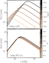 |
Fig. 2. Same as Fig. 1, but using the relations ϵB(δ) (top panel) and Tc(τT) (bottom panel) discussed in Sect. 3.1. |
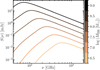 |
Fig. 3. Corona SEDs for different values of the SMBH mass. As MBH increases, the total flux increases and νSSA decreases. |
3.2. Studying sources at high redshift
The detection of mm coronal emission has so far been almost exclusively limited to local AGNs due to sensitivity limitations. This might be overcome in the case of high-z lensed quasars with high amplification factors μ and large MBH. Remarkably, an indication of coronal emission like this was found in APM 08279+5255, an AGN at z ≃ 3.9 hosting an SMBH with MBH ≈ 109.8 M⊙ (Yang et al. 2023), and a clear detection was recently reported in the lensed quasar RXJ1131−1231, located at z = 0.658 (Rybak et al. 2025).
In Fig. 4 we show the corona SEDs for a source with MBH = 109 M⊙ and μ = 10 located at different z values. The remaining parameters are the same as we used in Fig. 3. For sources at z > 1, the peak of the SED falls below 40 GHz, and their maximum flux density falls below 0.1 mJy, thus making their observation unfeasible for ALMA. Instead, these are good candidates for the upcoming Square Kilometer Array (SKA6). For conditions similar to those assumed here, we predict that the SKA-Mid could detect these sources up to z ∼ 4 with a ∼1 h integration (reaching sensitivities of ∼1 μJy).
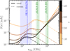 |
Fig. 4. Example SEDs for a source with MBH = 109 M⊙ and μ = 10 at different redshifts z. Arbitrary synchrotron and dust components were added to mimic more realistic SEDs. The frequency ranges for highly sensitive observatories are also shown. |
3.3. Analysis of the sample sources
We applied our model and fitting scheme to a sample of seven RQ AGNs that includes all sources for which strong indications of coronal activity have been reported in the literature (GRS 1734−292, IC 4329A, MCG+08−11−11, NGC 985, and NGC 1068), together with two sources for which high-resolution data from radio-cm to (sub)mm are available (MCG−06−30−15 and NGC 3227). For all sources, we performed a detailed bibliographic search for published flux densities and then included additional data from unpublished archival observations from various surveys. Namely, we searched for archival data with the Karl G. Jansky Very Large Array (VLA)7, and surveys accessed via the CIRADA image web cutout service8, in particular, the VLASS (Lacy et al. 2020), NVSS (Condon et al. 1998), and RACS (Hale et al. 2021). In Appendix B we provide a short description of each source, and in Tables B.1-B.7, we detail the data we used, including the flux densities and relevant angular sizes.
The SEDs of six sources and their fit are shown in Fig. 5. We left MCG+08−11−11 out of this part of the analysis because its corona component is not constrained by the currently available data (Fig. B.1). More details about the SED fitting procedure in each source are discussed in Appendix B, and the corresponding fit posteriors are provided in Figs. C.1–C.7.
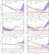 |
Fig. 5. Multi-frequency SEDs and model fitting of the RQ galaxies in the sample. Data from low-resolution observations were treated as upper limits and are shown with red arrows, and data from very high-resolution observations were treated as lower limits and are shown with green arrows (Sect. 2.2). Further details are provided in Appendix B. For NGC 3227, we also show an upper limit at 43 GHz (cyan arrow) that we did not use in the fitting due to its very high angular resolution, but the compact corona emission should still remain below this value for consistency. |
We summarise the results of the SED fitting of the two relevant corona parameters, rc and δ, in Fig. 6. The parameters range from rc = 60–250 and δ = 10−3–10−1, with median values of rc ≈ 133 and log δ ≈ −1.86 (δ ≈ 1.4%). The derived values of B range between 10–150 G, with a median of ≈20 G. We also find values of σ between 0.01–1, with a mean value of ≲0.1, which is roughly consistent with the assumption of a significantly magnetised medium (σ ∼ 1).
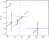 |
Fig. 6. Non-thermal particle content and corona sizes obtained for the sources in the sample via the SED fitting (with the parameters defined as in Sects. 2.1 and 2.2). The dashed grey lines mark the median values rc = 133 and log δ = −1.86. For the sources GRS 1734−292 and IC 4329A, the broad range in rc reflects the range in sizes derived in different epochs. |
We finally studied whether the peak of the corona SED was anti-correlated with the SMBH mass, as predicted in Sect. 3.1. We show a plot of these two quantities in Fig. 7. Although the sample is still very small, an indication of this anti-correlation can be seen.
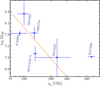 |
Fig. 7. Peak frequency of the corona component vs. the mass of the SMBH. The dotted line with the slope −0.37 shows the model prediction (Sect. 3.1). We note that the error bar of MBH is very small in NGC 1068 (Gallagher et al. 2024). |
3.4. MBH–L220 GHz correlation modelling
For a fixed value of MBH, we used our corona emission model to calculate the corona emission at a rest-frame frequency of 220 GHz. We repeated this calculation for a broad range of MBH and plot this relation in Fig. 8. One key prediction of our model is a slope change in the correlation at νLν ∼ 1039 erg s−1, related to the corona emission becoming optically thin at 220 GHz for SMBHs more massive than ∼108 M⊙ (Fig. 3).
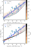 |
Fig. 8. Correlation between the luminosity at 220 GHz and the black hole mass. The points and the blue curve are taken from Ruffa et al. (2024); filled circles show sources with dynamical MBH measurements, and open squares represent sources with MBH derived using the MBH–σ⋆ relation (Ruffa et al. 2024). The upper limits are plotted in green for clarity. We also plot the sources we studied with pink stars (except for NGC 3227, which was already included in their sample). The colour-gradient curves are the corona luminosities calculated for the model parameters defined in Sect. 3.1, and using the approximate mean values of rc = 130 and log δ = −2.0 (Sect. 3.3). We explore different values of rc (top panel) and δ (bottom panel), covering the ranges derived for the sources in the sample. |
We compared our correlation with the empirical correlation reported by Ruffa et al. (2024). The result is shown in Fig. 8. In general, we can broadly explain the spread on the observed correlation when we take the parameter space available in δ and rc into account, which are the most relevant parameters for the corona emission. This supports the hypothesis that a physical connection underlies this correlation, although this still needs to be tested in more detail and with an increased sample size, in particular, at νLν ≲ 1037 erg s−1 and νLν ≳ 1040 erg s−1. In addition, when using a single frequency band, observations with a very high angular resolution are needed to isolate the (compact) coronal component from other galactic contributions, which can otherwise contaminate the flux densities at mm frequencies significantly. This additional non-coronal emission shifts the observed sources farther to the right in Fig. 8. We also note that some points lie significantly to the left of the correlation (in particular, around νLν ∼ 1038 erg s−1), suggesting that they are underluminous in mm wavelengths.
4. Discussion
The corona properties we derived in Sect. 3.3 agree roughly with what was reported by other authors in the literature (Behar et al. 2015; Inoue & Doi 2018), which raises two points. First, we note that the sizes inferred from the mm observations are consistently larger than those inferred from X-ray observations (Fabian et al. 2015) or microlensing (Rybak et al. 2025). Second, we note that the value we obtain of δ ≈ 1.4% agrees with the value required to explain the MeV background (Inoue et al. 2008, 2019). In addition, this value of δ corresponds to ϵB ∼ 0.5, leading to βB ∼ 10 (Sect. 2.1). We note that values of βB > 1 may challenge the ability of magnetic fields to sustain particle acceleration and heating in the corona (Inoue et al. 2024).
To suggest possible ways forward, we outline the main limitations of our multi-component SED fitting, both from the modelling perspective and from observational constraints. First, we highlight that we used a one-zone coronal emission model. Even though the assumption of a homogeneous emitter is most likely an oversimplification, it still yields results that are currently consistent with the observations. It remains extremely difficult to constrain more complex models (e.g. Raginski & Laor 2016) unless the optically thick part of the radio-mm SED is clearly detected. In most sources, this will require very deep observations with a high angular resolution at frequencies below 100 GHz. Notably, the correlation between the radio and X-ray luminosity is weaker at 22 GHz (Magno et al. 2025) than at 100 GHz (Ricci et al. 2023), consistent with the weaker coronal emission at 22 GHz predicted by our one-zone model. Another limitation of assuming a homogeneous spherical corona is that we cannot predict realistic images of it, although their characteristic sizes of below a few μas make them unresolvable with current facilities. As a final note on the coronae, we note that when observing very dust-obscured sources, we could expect absorption of its emission by dust at frequencies above ντ1, although this depends on the dust being along our line of sight to the corona.
Further limitations of the method we used here include that an AME component from spinning dust grains is not included, which might be relevant in sources that present a bump in the SED at ∼30 GHz (which is not the case for the sources in our sample). This component can be added at the expense of additional free parameters. We preferred to ignore the effects of f–f absorption (FFA) in the synchrotron component because the data at high angular resolution at low frequencies are limited, although this possibility is available in our code (an application of a clumpy absorption medium was presented in Mutie et al. 2025). In this regard, a more model-dependent approach might be adopted in which, under certain assumptions about the diffuse gas distribution, the FFA is linked to the f–f emission, but this should be properly tested on a large sample of galaxies that is not necessarily limited to RQ AGNs with corona emission. For this reason, we currently favour a more phenomenological approach in which the parameters that describe the FFA and f–f emission are not tied to further assumptions.
Finally, we highlight the observational challenges involved in studying the corona emission of RQ AGNs. From a fitting perspective, it is crucial to have a well-sampled SED from radio to FIR with consistent angular resolutions and uv-coverage. This ensures that the same scales are probed, although it is very challenging to obtain such a consistent dataset (so far only attempted in Mutie et al. 2025). High-resolution IR imaging is currently unavailable, which hinders our chances of constraining the dust component. The next-generation VLA (ngVLA9) is very promising due to the extremely good angular resolution and sensitivity to frequencies up to ∼100 GHz that it will provide. In the mm to sub-mm domain, ALMA will remain the most suitable observatory.
One of the most difficult issues to address in the SED fitting is the corona variability on timescales of days. The most extreme case of variability so far was found in IC 4329A, in which the mm flux density varied by a factor of ∼3 and the inferred corona size by a factor of ∼2, while δ remained about constant (Shablovinskaya et al. 2024). Other sources have shown even less variability, and thus, the corresponding change in the coronal parameters should be even smaller. This is difficult to assess, however, due to the very limited studies of this phenomenon to date and because a broad frequency coverage is needed for a good SED fit. In this regard, the prospects for the ALMA Wide Sensitivity Upgrade are particularly promising, as it will allow us to obtain a broad bandwidth in a single epoch. This is particularly useful at ∼100 GHz (as shown in Shablovinskaya et al. 2024). Complementing this with simultaneous hard X-ray observations is ideal because it can further reduce the uncertainty in the corona parameters τT and k Tc, although this should not be a deciding factor in most cases (Fig. 2).
5. Conclusions
We presented a comprehensive study of mm wave coronal emission in SMBH coronae. We first introduced a model for calculating the synchrotron emission from an SMBH corona based on Inoue & Doi (2018), coupled with an SED fitting scheme optimised for realistic datasets. That is, we minimised the number of free parameters in the model by introducing a physically motivated parametrisation of the magnetic field intensity and an empirical parametrisation for the opacity and temperature of the corona. We applied our model systematically to the five RQ AGNs for which coronal mm emission had been reported, together with two additional RQ AGNs with excellent multi-wavelength data from radio-cm to sub-mm frequencies. Our SED fitting results suggest that the coronae have non-thermal particle energy density fractions of 0.5–10% and radii of 60–250 Rg, from which we inferred typical magnetic fields of 10–60 G. These sets of parameters can also explain the putative correlation between MBH and mm-wave luminosity presented in Ruffa et al. (2024). This opens the possibility of estimating MBH via mm wave observations in systems that are difficult to observe at other wavelengths, such as extremely obscured sources. Another suggested application of this approach is to measure faint coronal emission in high-z lensed quasars using next-generation radio observatories. We conclude that multi-frequency continuum observations spanning from radio to far-IR frequencies, with a particular emphasis on the mm band, can be used as direct probes of the physical properties of SMBH coronae. The knowledge gained from these observations can have direct applications for other studies related to accretion disc coronae, such as in XRBs and tidal disruption events. Moreover, the detailed information on electron acceleration in the corona can help multi-messenger emission modelling and allow us to derive more robust predictions of neutrino sources or to verify neutrino detections.
All frequencies are given in the rest frame. For spectral indices, we adopt the convention Sν ∝ να.
https://github.com/bmargalit/thermal-synchrotron, with the correction later introduced in Margalit & Quataert (2024).
If a two-temperature plasma is assumed for the corona, for rc ∼ 140, we expect an ion temperature of Ti ∼ 1.1 MeV (e.g. Eq. (1) in Inoue et al. 2024), and thus, a total thermal pressure of Pth ∼ (1 + Ti/Tc) Uth, e/a(Θ)∼5Uth, e.
Acknowledgments
We thank the referee for their comments and suggestions to improve the manuscript. SdP, CY, SA and SK gratefully acknowledge funding from the European Research Council (ERC) under the European Union’s Horizon 2020 research and innovation programme (grant agreement No 789410, PI: S. Aalto). SGB acknowledges support from the Spanish grant PID2022-138560NB-I00, funded by MCIN AEI/10.13039/501100011033/FEDER, EU. MPS acknowledges support under grants RYC2021-033094-I, CNS2023-145506 and PID2023-146667NB-I00 funded by MCIN/AEI/10.13039/501100011033 and the European Union NextGenerationEU/PRTR. JBT acknowledges support from the DFG, via the Collaborative Research Center SFB1491 “Cosmic Interacting Matters – from Source to Signal” (project no. 445052434). IGB is supported by the Programa Atracción de Talento Investigador “César Nombela” via grant 2023-T1/TEC-29030 funded by the Community of Madrid. This paper makes use of the following ALMA data: ADS/JAO.ALMA#2017.1.00236.S, ADS/JAO.ALMA#2019.1.00618.S, ADS/JAO.ALMA#2019.1.01230.S, ADS/JAO.ALMA#2015.1.01047.S, ADS/JAO.ALMA#2023.1.00121.S, ADS/JAO.ALMA#2021.1.00812.S. ALMA is a partnership of ESO (representing its member states), NSF (USA) and NINS (Japan), together with NRC (Canada), NSTC and ASIAA (Taiwan), and KASI (Republic of Korea), in cooperation with the Republic of Chile. The Joint ALMA Observatory is operated by ESO, AUI/NRAO and NAOJ. This research has made use of the CIRADA cutout service at cutouts.cirada.ca, operated by the Canadian Initiative for Radio Astronomy Data Analysis (CIRADA). CIRADA is funded by a grant from the Canada Foundation for Innovation 2017 Innovation Fund (Project 35999), as well as by the Provinces of Ontario, British Columbia, Alberta, Manitoba and Quebec, in collaboration with the National Research Council of Canada, the US National Radio Astronomy Observatory and Australia’s Commonwealth Scientific and Industrial Research Organisation.
References
- Alonso-Herrero, A., García-Burillo, S., Pereira-Santaella, M., et al. 2019, A&A, 628, A65 [NASA ADS] [CrossRef] [EDP Sciences] [Google Scholar]
- An, F., Vaccari, M., Best, P. N., et al. 2024, MNRAS, 528, 5346 [NASA ADS] [CrossRef] [Google Scholar]
- Ashton, G., Hübner, M., Lasky, P. D., et al. 2019, ApJS, 241, 27 [NASA ADS] [CrossRef] [Google Scholar]
- Balbus, S. A., & Hawley, J. F. 1998, Rev. Mod. Phys., 70, 1 [Google Scholar]
- Bambi, C., Brenneman, L. W., Dauser, T., et al. 2021, Space Sci. Rev., 217, 65 [CrossRef] [Google Scholar]
- Bauer, F. E., Arévalo, P., Walton, D. J., et al. 2015, ApJ, 812, 116 [Google Scholar]
- Behar, E., Baldi, R. D., Laor, A., et al. 2015, MNRAS, 451, 517 [NASA ADS] [CrossRef] [Google Scholar]
- Behar, E., Vogel, S., Baldi, R. D., Smith, K. L., & Mushotzky, R. F. 2018, MNRAS, 478, 399 [CrossRef] [Google Scholar]
- Beloborodov, A. M. 2017, ApJ, 850, 141 [NASA ADS] [CrossRef] [Google Scholar]
- Bontempi, P., Giroletti, M., Panessa, F., Orienti, M., & Doi, A. 2012, MNRAS, 426, 588 [NASA ADS] [CrossRef] [Google Scholar]
- Cangemi, F., Beuchert, T., Siegert, T., et al. 2021, A&A, 650, A93 [NASA ADS] [CrossRef] [EDP Sciences] [Google Scholar]
- Ciesla, L., Boselli, A., Smith, M. W. L., et al. 2012, A&A, 543, A161 [NASA ADS] [CrossRef] [EDP Sciences] [Google Scholar]
- Condon, J. J., Cotton, W. D., Greisen, E. W., et al. 1998, AJ, 115, 1693 [Google Scholar]
- Dey, S., Goyal, A., Małek, K., & Díaz-Santos, T. 2024, ApJ, 966, 61 [Google Scholar]
- Dickinson, C., Ali-Haïmoud, Y., Barr, A., et al. 2018, New Astron. Rev., 80, 1 [CrossRef] [Google Scholar]
- Draine, B. T. 2011, Physics of the Interstellar and Intergalactic Medium [Google Scholar]
- Eichmann, B., Oikonomou, F., Salvatore, S., Dettmar, R.-J., & Tjus, J. B. 2022, ApJ, 939, 43 [NASA ADS] [CrossRef] [Google Scholar]
- Fabian, A. C., Lohfink, A., Kara, E., et al. 2015, MNRAS, 451, 4375 [Google Scholar]
- Fang, K., Halzen, F., Heinz, S., & Gallagher, J. S. 2024, ApJ, 975, L35 [Google Scholar]
- Fernández-Torreiro, M., Génova-Santos, R. T., Rubiño-Martín, J. A., et al. 2024, MNRAS, 527, 11945 [Google Scholar]
- Foreman-Mackey, D., Hogg, D. W., Lang, D., & Goodman, J. 2013, PASP, 125, 306 [Google Scholar]
- Gallagher, J. S., Kotulla, R., Laufman, L., et al. 2024, ApJS, 274, 3 [Google Scholar]
- Gallimore, J. F., Impellizzeri, C. M. V., Aghelpasand, S., et al. 2024, ApJ, 975, L9 [Google Scholar]
- García-Burillo, S., Combes, F., Ramos Almeida, C., et al. 2016, ApJ, 823, L12 [Google Scholar]
- Grošelj, D., Hakobyan, H., Beloborodov, A. M., Sironi, L., & Philippov, A. 2024, Phys. Rev. Lett., 132, 085202 [CrossRef] [Google Scholar]
- Haardt, F., & Maraschi, L. 1991, ApJ, 380, L51 [Google Scholar]
- Hale, C. L., McConnell, D., Thomson, A. J. M., et al. 2021, PASA, 38 [Google Scholar]
- Heesen, V., Staffehl, M., Basu, A., et al. 2022, A&A, 664, A83 [NASA ADS] [CrossRef] [EDP Sciences] [Google Scholar]
- IceCube Collaboration (Abbasi, R., et al.) 2022, Science, 378, 538 [CrossRef] [PubMed] [Google Scholar]
- Ichikawa, K., Ricci, C., Ueda, Y., et al. 2019, ApJ, 870, 31 [NASA ADS] [CrossRef] [Google Scholar]
- Imanishi, M., Nakanishi, K., & Izumi, T. 2016, AJ, 152, 218 [Google Scholar]
- Ingram, A., Ewing, M., Marinucci, A., et al. 2023, MNRAS, 525, 5437 [CrossRef] [Google Scholar]
- Inoue, Y., & Doi, A. 2014, PASJ, 66, L8 [NASA ADS] [CrossRef] [Google Scholar]
- Inoue, Y., & Doi, A. 2018, ApJ, 869, 114 [Google Scholar]
- Inoue, Y., Totani, T., & Ueda, Y. 2008, ApJ, 672, L5 [Google Scholar]
- Inoue, Y., Khangulyan, D., Inoue, S., & Doi, A. 2019, ApJ, 880, 40 [Google Scholar]
- Inoue, Y., Khangulyan, D., & Doi, A. 2020, ApJ, 891, L33 [Google Scholar]
- Inoue, Y., Takasao, S., & Khangulyan, D. 2024, PASJ, 76, 996 [Google Scholar]
- Jana, A., Ricci, C., Venselaar, S. M., et al. 2025, A&A, 699, A62 [NASA ADS] [CrossRef] [EDP Sciences] [Google Scholar]
- Kamraj, N., Brightman, M., Harrison, F. A., et al. 2022, ApJ, 927, 42 [NASA ADS] [CrossRef] [Google Scholar]
- Karpouzas, K., Méndez, M., García, F., et al. 2021, MNRAS, 503, 5522 [NASA ADS] [CrossRef] [Google Scholar]
- Kawamuro, T., Ricci, C., Imanishi, M., et al. 2022, ApJ, 938, 87 [NASA ADS] [CrossRef] [Google Scholar]
- Kornecki, P., Peretti, E., del Palacio, S., Benaglia, P., & Pellizza, L. J. 2022, A&A, 657, A49 [NASA ADS] [CrossRef] [EDP Sciences] [Google Scholar]
- Koss, M., Trakhtenbrot, B., Ricci, C., et al. 2017, ApJ, 850, 74 [Google Scholar]
- Kun, E., Bartos, I., Tjus, J. B., et al. 2024, Phys. Rev. D, 110, 123014 [Google Scholar]
- Kylafis, N. D., Reig, P., & Tsouros, A. 2023, A&A, 679, A81 [NASA ADS] [CrossRef] [EDP Sciences] [Google Scholar]
- Lacki, B. C. 2013, MNRAS, 431, 3003 [Google Scholar]
- Lacki, B. C., & Thompson, T. A. 2010, ApJ, 717, 196 [Google Scholar]
- Lacy, M., Baum, S. A., Chandler, C. J., et al. 2020, PASP, 132, 035001 [Google Scholar]
- Laor, A., & Behar, E. 2008, MNRAS, 390, 847 [NASA ADS] [CrossRef] [Google Scholar]
- Magno, M., Smith, K. L., Wong, O. I., et al. 2025, ApJ, 981, 202 [Google Scholar]
- Margalit, B., & Quataert, E. 2021, ApJ, 923, L14 [NASA ADS] [CrossRef] [Google Scholar]
- Margalit, B., & Quataert, E. 2024, ApJ, 977, 134 [Google Scholar]
- Marti, J., Mirabel, I. F., Chaty, S., & Rodriguez, L. F. 1998, A&A, 330, 72 [NASA ADS] [Google Scholar]
- Mejía-Restrepo, J. E., Trakhtenbrot, B., Koss, M. J., et al. 2022, ApJS, 261, 5 [CrossRef] [Google Scholar]
- Merten, L., Becker Tjus, J., Eichmann, B., & Dettmar, R.-J. 2017, Astropart. Phys., 90, 75 [NASA ADS] [CrossRef] [Google Scholar]
- Michiyama, T., Inoue, Y., Doi, A., et al. 2024, ApJ, 965, 68 [NASA ADS] [CrossRef] [Google Scholar]
- Murase, K., Kimura, S. S., & Mészáros, P. 2020, Phys. Rev. Lett., 125, 011101 [Google Scholar]
- Murphy, E. J., Condon, J. J., Schinnerer, E., et al. 2011, ApJ, 737, 67 [Google Scholar]
- Murphy, E. J., Dong, D., Momjian, E., et al. 2018, ApJS, 234, 24 [NASA ADS] [CrossRef] [Google Scholar]
- Murphy, E. J., Hensley, B. S., Linden, S. T., et al. 2020, ApJ, 905, L23 [Google Scholar]
- Mutie, I. M., del Palacio, S., Beswick, R. J., et al. 2025, MNRAS, 539, 808 [Google Scholar]
- Nättilä, J. 2024, Nat. Commun., 15, 7026 [Google Scholar]
- Özel, F., Psaltis, D., & Narayan, R. 2000, ApJ, 541, 234 [Google Scholar]
- Pal, I., & Stalin, C. S. 2023, MNRAS, 518, 2529 [Google Scholar]
- Panessa, F., Baldi, R. D., Laor, A., et al. 2019, Nat. Astron., 3, 387 [Google Scholar]
- Panessa, F., Chiaraluce, E., Bruni, G., et al. 2022, MNRAS, 515, 473 [Google Scholar]
- Petrucci, P. O., Piétu, V., Behar, E., et al. 2023, A&A, 678, L4 [NASA ADS] [CrossRef] [EDP Sciences] [Google Scholar]
- Poojon, P., Chung, A., Hoang, T., et al. 2024, ApJ, 963, 88 [Google Scholar]
- Raginski, I., & Laor, A. 2016, MNRAS, 459, 2082 [CrossRef] [Google Scholar]
- Raimundo, S. I., Davies, R. I., Gandhi, P., et al. 2013, MNRAS, 431, 2294 [Google Scholar]
- Ramírez-Olivencia, N., Varenius, E., Pérez-Torres, M., et al. 2022, A&A, 658, A4 [NASA ADS] [CrossRef] [EDP Sciences] [Google Scholar]
- Ricci, C., Ho, L. C., Fabian, A. C., et al. 2018, MNRAS, 480, 1819 [NASA ADS] [CrossRef] [Google Scholar]
- Ricci, C., Chang, C.-S., Kawamuro, T., et al. 2023, ApJ, 952, L28 [NASA ADS] [CrossRef] [Google Scholar]
- Romero, G. E., Vieyro, F. L., & Chaty, S. 2014, A&A, 562, L7 [NASA ADS] [CrossRef] [EDP Sciences] [Google Scholar]
- Ruffa, I., Davis, T. A., Elford, J. S., et al. 2024, MNRAS, 528, L76 [Google Scholar]
- Rybak, M., Sluse, D., Gupta, K., et al. 2025, A&A, in press, https://doi.org/10.1051/0004-6361/202554595 [Google Scholar]
- Sani, E., Davies, R. I., Sternberg, A., et al. 2012, MNRAS, 424, 1963 [NASA ADS] [CrossRef] [Google Scholar]
- Sargent, A. J., van der Horst, A. J., Johnson, M. C., et al. 2025, ApJ, 986, 194 [Google Scholar]
- Shablovinskaya, E., Ricci, C., Chang, C. S., et al. 2024, A&A, 690, A232 [NASA ADS] [CrossRef] [EDP Sciences] [Google Scholar]
- Shimwell, T. W., Röttgering, H. J. A., Best, P. N., et al. 2017, A&A, 598, A104 [NASA ADS] [CrossRef] [EDP Sciences] [Google Scholar]
- Sironi, L., & Beloborodov, A. M. 2020, ApJ, 899, 52 [NASA ADS] [CrossRef] [Google Scholar]
- Smith, K. L., Mushotzky, R. F., Koss, M., et al. 2020, MNRAS, 492, 4216 [NASA ADS] [CrossRef] [Google Scholar]
- The Fermi-LAT Collaboration (Wang, J.-M., et al.) 2020, MNRAS, 492, 4216 [NASA ADS] [CrossRef] [Google Scholar]
- Tortosa, A., Marinucci, A., Matt, G., et al. 2017, MNRAS, 466, 4193 [NASA ADS] [Google Scholar]
- Tortosa, A., Bianchi, S., Marinucci, A., Matt, G., & Petrucci, P. O. 2018, A&A, 614, A37 [NASA ADS] [CrossRef] [EDP Sciences] [Google Scholar]
- Tortosa, A., Ricci, C., Shablovinskaia, E., et al. 2024, A&A, 687, A51 [NASA ADS] [CrossRef] [EDP Sciences] [Google Scholar]
- Urry, C. M., & Padovani, P. 1995, PASP, 107, 803 [NASA ADS] [CrossRef] [Google Scholar]
- Yang, C., Omont, A., Martín, S., et al. 2023, A&A, 680, A95 [NASA ADS] [CrossRef] [EDP Sciences] [Google Scholar]
- Zdziarski, A. A., Jourdain, E., Lubiński, P., et al. 2021, ApJ, 914, L5 [NASA ADS] [CrossRef] [Google Scholar]
Appendix A: Synchrotron emission from a thermal population of electrons
We explore in more detail whether it is feasible for thermal electrons alone to produce appreciable synchrotron emission, compatible with the mm emission detected in several sources. The number of relativistic electrons in a thermal distribution strongly depends on the temperature of the plasma. We, therefore, calculated SEDs for corona temperatures ranging from 200 to 400 keV, shown in Fig. A.1. We note that values of kTc ∼ 500 keV could be unsustainable due to runaway pair production. For kTc < 200 keV, there are simply not enough relativistic electrons to emit detectable synchrotron, and even for kTc ≳ 300 keV this emission is quite faint. For reference, we also show the total emission, including a very small fraction of non-thermal electrons, δ = 10−3. The non-thermal electrons completely dominate the emission for kTc < 300 keV. The only case in which the emission from thermal electrons could be dominant is for extremely high corona temperatures kTc ∼ 400 keV and low values of δ ≲ 10−3. However, such a scenario (kTc ∼ 400 keV, τT ∼ 1, rc ∼ 120, B ∼ 100 G) is energetically very demanding, still produces faint mm emission, and would most likely overpredict the X-ray luminosity. We thus conclude that scenarios with kTc < 200 keV and δ > 10−3 are far more promising for explaining the mm emission in RQ AGNs.
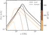 |
Fig. A.1. SEDs for different values of kTc for the same parameters as in Sect. 3.1 but fixing δ = 10−3. Dashed lines represent the emission from thermal electrons, and solid lines represent the total emission. |
Appendix B: Source sample
In the following, we provide a short description of the sources analysed in this work and their SED fitting. The fluxes reported in this work are a combination of archival and proprietary observations. As such, the datasets are non-simultaneous, with typical timespans of several years. Among the archives used, we highlight the LoTSS survey with LOFAR (Shimwell et al. 2017), the RACS survey with ASKAP (Hale et al. 2021), and the VLASS survey with the VLA (Lacy et al. 2020). We note that all flux density errors presented in the tables include only the statistical errors; for the inclusion of systematic errors, we refer to Sect. 2.2. For flux densities that are not taken from the literature, we also specify the observatory that took the data we used. We used CARTA10 to obtain the flux density fitting a Gaussian profile.
For all sources, we also calculate the predicted X-ray luminosities by plugging the luminosity at 100 GHz from our model fitting into the correlation from Ricci et al. (2023) between the 100-GHz luminosity and the 14–150 keV luminosity. We note that, in principle, we could use the mm luminosity coming only from the corona (which should be the one scaling with the X-ray luminosity), but we prefer to keep consistency with how the correlations in Ricci et al. (2023) were derived, in which the total emission at 100 GHz was used, even though this can have a significant contribution from non-coronal components depending on the source. In addition, in some cases, the corona component peaks at frequencies significantly above 100 GHz, and we speculate that in those cases the correlation of Kawamuro et al. (2022) between the 230-GHz luminosity and the 14–150 keV luminosity can be more accurate.
B.1. GRS 1734−292
This galaxy is located at a distance of 84 Mpc (z = 0.021) and is a known hard X-ray source (e.g. Tortosa et al. 2017). Moreover, Michiyama et al. (2024) found a ≳50% increase in the source 100-GHz flux in timescales of days; this mm flux variability is a strong indication of the origin of the mm flux in the corona (we refer to Shablovinskaya et al. 2024, for an in-depth discussion of this reasoning). Unfortunately, the source also presents a weak radio jet on angular scales of a few arcseconds, making it difficult to build a consistent SED, as the presence of diffuse emission leads to an artificially steep spectrum if the lower resolution data at lower frequencies are included. Due to these limitations on the dataset, and the fact that f–f emission cannot dominate at ∼100 GHz, we simply opt to remove the f–f component and to fix αsy = 0.75 as in Michiyama et al. (2024). In addition, the lack of data above 230 GHz prevents us from constraining the dust component, so we fix β = 1.78 and ντ1 = 800 GHz. We adopt a value of MBH = 107.84 M⊙ (Mejía-Restrepo et al. 2022). Furthermore, we fix τT = 2.98 and kTc = 12 keV, as derived by Tortosa et al. (2017). We fit the flux densities listed in Table B.1. We obtain rc = 112 ± 14 (Rc ≈ 0.5 ld) and log δ = −1.74 ± 0.13, leading to B ∼ 20 G and σ ∼ 0.011; the corona peaks at νp = 130 ± 14 GHz with a peak flux density of Sp = 0.91 ± 0.11 mJy and has a luminosity of Lc ≈ 4 × 1039 erg s−1. The predicted X-ray luminosity is L14 − 150 keV ≈ 8 × 1043 erg s−1, corresponding to λEdd ∼ 0.004. The cornerplot of the fit is shown in Fig. C.1.
In addition, we explore the change in the corona parameters during the epoch of higher flux, when there are only observations at ALMA B3. Thus, we choose to fix log δ = −1.74 as in the previous epoch, and the fit yields rc = 178 ± 9. This suggests that the size of the corona can be much larger than the one derived for the better-sampled epoch, although it is not possible at this stage to define which value is more representative of the average size of the mm-emitting corona.
Data used for the SED of GRS 1734−292.
B.2. IC 4329A
This is a very well-studied source both in radio and X-rays (e.g. Inoue & Doi 2018; Ingram et al. 2023; Tortosa et al. 2024; Shablovinskaya et al. 2024), showing convincing evidence of a hybrid corona. In fact, this source is one of the first two sources for which a bump in the SED around ∼100 GHz was detected (Inoue & Doi 2018). Moreover, Shablovinskaya et al. (2024) proved that the emission at 100 GHz is significantly variable on daily timescales. We adopt MBH = 6.8 × 10⁷ M⊙ as in Shablovinskaya et al. (2024), and fit our model to the same dataset presented in Table 1 of Inoue & Doi (2018). To present a consistent approach as with the other sources, we fix p = 2.7 and τT = 0.25 and kTc ≈ 166 K. We note that, observationally, the values of τT and kTc are not well constrained and are also variable (e.g. Tortosa et al. 2024), but the specific values adopted should not play a significant role in the fitting (as shown in Sect. 3.1). The SED is poorly constrained between 10 and 100 GHz; we therefore fix αsy = −0.59 as in Inoue & Doi (2018). We obtain  and
and  (Rc ≈ 1 ld), leading to B ∼ 9.3 G and σ ∼ 0.06. The corona component peaks at νp = 90 ± 20 GHz, with a peak flux density of Sp = 4.2 ± 1.1 mJy, and has a luminosity of Lc ≈ 7 × 1039 erg s−1. The cornerplot of the fit is shown in Fig. C.2. The predicted X-ray luminosity is L14 − 150 keV ≈ 2 × 1044 erg s−1, corresponding to λEdd ∼ 0.02. Alternatively, the SED fit to the multiple epochs of 100-GHz observations presented in Shablovinskaya et al. (2024) yielded a broader range of sizes of the corona of ∼170–300 Rg.
Same as Table B.1 but for IC 4329A.
B.3. MCG−06−30−15
This RQ-AGN is located at a distance of D = 34 Mpc and hosts an SMBH with log MBH ≈ 7.3 (Raimundo et al. 2013, and references therein). From hard X-ray observations it is inferred kTc ≈ 63 keV and τT = 0.27. An analysis of the VLA fluxes from images at different resolutions indicates that there is significant diffuse emission on scales > 0.3″ (Table B.3).
We cannot constrain the dust component properly due to the lack of data at ν > 300 GHz with comparable resolution. Following Kawamuro et al. (2022), we assume that the dust contribution is not significant at mm wavelengths given the very high angular resolution of the observations. We thus fix the dust component normalization to an arbitrary low value. In addition, trying to fit the spectral index p leads to a solution that hits the hard limit on the priors, and we thus fix p = 2.1. We obtain rc = 115 ± 6 (Rc ≈ 0.13 ld) and log δ = −1.98 ± 0.06, leading to B ∼ 20.9 G and σ ∼ 0.036. The corona component peaks at νp = 133 ± 6 GHz, with a peak flux density of Sp = 0.64 ± 0.06 mJy, and has a bolometric synchrotron luminosity of Lc ≈ 3 × 1038 erg s−1. The predicted X-ray luminosity is L14 − 150 keV ∼ 8 × 1043 erg s−1, corresponding to an Eddington ratio of λEdd ∼ 0.003. The cornerplot of the fit is shown in Fig. C.3.
Same as Table B.1 but for MCG−06−30−15.
B.4. MCG+08−11−11
This LIRG source is located at z = 0.02 and hosts an SMBH with a mass of log MBH = 7.81 (Koss et al. 2017). This is a well-known hard X-ray source, and Petrucci et al. (2023) showed evidence of a correlated variability in the hard X-ray and mm emission at 100 GHz (using NOEMA observations). In Smith et al. (2020), it is listed as a jetted source at 22 GHz. VLA images at 8.5 and 14.9 GHz show that the inner structure has three point-like sources within 0.5", plus diffuse emission on larger scales. For this reason, we integrate the flux within a ≈1" region at all frequencies. Morevoer, Pal & Stalin (2023) measured kTc∼30–60 keV, suggesting that the source has τT ≳ 1; we fix τT = 1.5. The fact that the ∼100-GHz emission reported by Petrucci et al. (2023) is variable on hour-timescales indicates that the corona contribution is non-negligible at this frequency. CARMA observations at 100 GHz with a 1"-resolution indicate a flux density of 7.5 mJy (Behar et al. 2018), which is significantly lower than the flux density of 18 mJy reported by (Petrucci et al. 2023). We fixed the dust component parameters β = 1.78 and ντ1 = 800 GHz. The corona SED is, unfortunately, very poorly constrained, and a robust fit cannot be addressed at this stage without high-resolution observations at frequencies > 100 GHz. Nonetheless, we can at least confirm that the observations are consistent with a corona of rc ∼ 260 (Rc ∼ 1 ld) and log δ ∼ −1.4 (yielding B ∼ 30 G). The predicted X-ray luminosity is L14 − 150 keV ∼ 3 × 1044 erg s−1, corresponding to an Eddington ratio of λEdd ∼ 0.035. The SED is shown in Fig. B.1 and the cornerplot of the fit is shown in Fig. C.4.
Same as Table B.1 but for MCG+08−11−11.
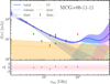 |
Fig. B.1. Same as Fig. 5 but for MCG+08−11−11. The corona component is not inferred from the SED shape, but rather from the variability (Petrucci et al. 2023). |
B.5. NGC 985
This galaxy located at D ≈ 190 Mpc hosts an SMBH with MBH = 2.2 × 10⁸ M⊙ (Inoue & Doi 2018, and references therein). Inoue & Doi (2018) reported an excess in the SED of this source at ∼100 GHz from which they inferred the presence of a corona. The dust component is essentially unconstrained due to a very bright FIR flux from the whole galaxy (Ichikawa et al. 2019). The high-resolution ALMA data favours a corona with a harder electron population, consistent with p ≈ 2.1 (Inoue & Doi 2018). Trying to fit this parameter hits the lower limit in the priors, and thus we fix it to p = 2.1. Following Inoue & Doi (2018), we also fix kTc = 29 keV and τT = 3.5. The inferred properties of the corona are:  (Rc ≈ 1.4 ld) and
  , leading to B ∼ 14.4 G and σ ∼ 0.014. The corona SED component peaks at νp = 100 ± 15 GHz, with a peak flux density of Sp = 1.4 ± 0.2 mJy, and has a bolometric synchrotron luminosity of Lc ≈ 4 × 1040 erg s−1. We estimate a hard X-ray luminosity L14 − 150 keV ≈ 4 × 1045 erg s−1, corresponding to an Eddington ratio of λEdd ∼ 0.011. The cornerplot of the fit is shown in Fig. C.5 and the data used is listed in Table B.5.
Same as Table B.1 but for NGC 985.
B.6. NGC 1068
This galaxy is located at D ≈ 14.6 Mpc (z = 0.0033) and hosts an SMBH with MBH = (1.66 ± 0.01)×107 M⊙ (Gallimore et al. 2024). This source has been the subject of very extensive research, given that it was the first RQ galaxy to be identified as a neutrino source (IceCube Collaboration 2022). It has also been extensively studied in X-rays, revealing the presence of a corona (e.g. Bauer et al. 2015). Furthermore, Inoue et al. (2020) modelled the radio continuum data and concluded that the synchrotron emission from the corona was responsible for the sub-mm emission detected by ALMA, which means that the corona peaks at a rather high frequency in this source compared to others. In a more recent work, Mutie et al. (2025) presented a consistent SED of the source matched in resolution and uv-coverage, confirming the presence of corona emission. For completeness, we reproduce the fluxes from their work in Table B.6.
The nuclear region of this source is particularly complex, and so is its SED at low frequencies (Mutie et al. 2025). For this reason, here we consider only high-resolution observations at ν ≥ 15 GHz. Due to the lack of FIR data to constrain the dust component, we fix β = 1.78 and ντ1 = 800 GHz as with the other sources. We refer to García-Burillo et al. (2016) for a discussion of the dust emission, although we caution that these authors did not take into account the coronal emission in their analysis. In addition, we fix αsy = −0.5 as otherwise the spectral index hits the hard limit set on −0.5. We obtain rc = 67.5 ± 5.5 (Rc ≈ 0.065 ld) and log δ = −0.98 ± 0.13, leading to B ∼ 158 G and σ ∼ 1.1. The corona SED peaks at νp ≃ 568 ± 55 GHz, with a peak flux density of Sp = 10.1 ± 1.9 mJy, and has a bolometric synchrotron luminosity of Lc ≈ 4.4 × 1039 erg s−1. Given that the peak frequency is much greater than 100 GHz, we estimate the hard X-ray luminosity using the relation from Kawamuro et al. (2022); we obtain a luminosity L14 − 150 keV ≈ 2.3 × 1043 erg s−1, corresponding to an Eddington ratio of λEdd ∼ 0.011. The cornerplot of the fit is shown in Fig. C.6. We note that this fit is quite similar to the one obtained by Inoue et al. (2020) and Mutie et al. (2025).
Same as Table B.1 but for NGC 1068.
B.7. NGC 3227
This galaxy located at D ≈ 23 Mpc (Ricci et al. 2023) hosts a MBH = 4.2 × 10⁷ M⊙ SMBH (Behar et al. 2015). Behar et al. (2015) showed that this source has a significant excess at ∼100 GHz. Sani et al. (2012) reported its flux density at 3 mm as observed by the Plateau de Bure with a ∼1" resolution. In addition, flux densities from ALMA observations at B6 and B7 were reported in Alonso-Herrero et al. (2019). According to the very high angular resolution observations at B3 in Ricci et al. (2023), the flux from the core region is ∼0.85 mJy. The dust component is poorly constrained due to a very bright FIR flux from the whole galaxy (Ciesla et al. 2012). However, Alonso-Herrero et al. (2019) fitted the IR SED with a dust model that has a flux of ∼10 mJy at 103 GHz (their Fig. 4), so that we can at least check that our model fitting is consistent with that derived independently using dust modelling of mid-IR low-resolution observations. Unfortunately, it is not possible to fit a dataset with very high angular resolution (< 0.1″) due to the limited number of data points. We thus use as reference points with resolutions ∼0.4"–1", which is not optimal for detecting the relatively faint corona emission. Thus, the properties of the corona are only loosely constrained as  (Rc ≈ 0.06 ld) and
  , leading to B ∼ 46 G and σ ∼ 0.09. The corona SED component peak is very poorly constrained at νp = 233 ± 91 GHz, with a peak flux density of Sp = 0.94 ± 0.48 mJy, and has a bolometric synchrotron luminosity of Lc ≈ 3 × 1038 erg s−1. Interestingly, the source is undetected in Q band with the VLA in A array configuration (project code AG568), giving an UL to the compact emission produced at 43.3 GHz, which is consistent with the SED fit of the corona component. We estimate a hard X-ray luminosity L14 − 150 keV ≈ 8 × 1042 erg s−1, corresponding to an Eddington ratio of λEdd ∼ 0.004. The cornerplot of the fit is shown in Fig. C.7.
Same as Table B.1 but for NGC 3227.
Appendix C: Parameter space and cornerplots
We sample a broad range in the parameter space to ensure that all possible solutions are explored. A list of parameters and their allowed ranges is presented in Table 1. We highlight that we fit the logarithm of those parameter that can spread over several orders of magnitude (namely the normalisations and δ).
We show the cornerplots for all the SED fits in Figs. C.1–C.7. The top panels of each plot show the 1-D distributions of the individual parameters, with the orange line marking the position of the median, and the dashed lines the 1-σ confidence interval.
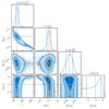 |
Fig. C.1. Cornerplot for the posteriors of the SED fit for GRS 1734−292. |
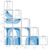 |
Fig. C.2. Cornerplot for the posteriors of the SED fit for IC 4329A. |
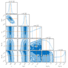 |
Fig. C.3. Cornerplot for the posteriors of the SED fit for MCG−06−30−15. |
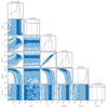 |
Fig. C.4. Cornerplot for the posteriors of the SED fit for MCG+08−11−11. |
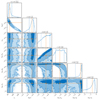 |
Fig. C.5. Cornerplot for the posteriors of the SED fit for NGC 985. |
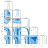 |
Fig. C.6. Cornerplot for the posteriors of the SED fit for NGC 1068. |
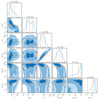 |
Fig. C.7. Cornerplot for the posteriors of the SED fit for NGC 3227. |
All Tables
All Figures
|
Fig. 1. Corona SEDs in which only one parameter was varied at a time, as indicated in the colour bar of each panel. The fiducial values are D = 100 Mpc, MBH = 108 M⊙, τT = 0.25, kTc = 166 keV, rc = 130, log ϵB = 0, log δ = −1.5, and p = 2.7. More details are discussed in Sect. 3.1. |
| In the text | |
|
Fig. 2. Same as Fig. 1, but using the relations ϵB(δ) (top panel) and Tc(τT) (bottom panel) discussed in Sect. 3.1. |
| In the text | |
|
Fig. 3. Corona SEDs for different values of the SMBH mass. As MBH increases, the total flux increases and νSSA decreases. |
| In the text | |
|
Fig. 4. Example SEDs for a source with MBH = 109 M⊙ and μ = 10 at different redshifts z. Arbitrary synchrotron and dust components were added to mimic more realistic SEDs. The frequency ranges for highly sensitive observatories are also shown. |
| In the text | |
|
Fig. 5. Multi-frequency SEDs and model fitting of the RQ galaxies in the sample. Data from low-resolution observations were treated as upper limits and are shown with red arrows, and data from very high-resolution observations were treated as lower limits and are shown with green arrows (Sect. 2.2). Further details are provided in Appendix B. For NGC 3227, we also show an upper limit at 43 GHz (cyan arrow) that we did not use in the fitting due to its very high angular resolution, but the compact corona emission should still remain below this value for consistency. |
| In the text | |
|
Fig. 6. Non-thermal particle content and corona sizes obtained for the sources in the sample via the SED fitting (with the parameters defined as in Sects. 2.1 and 2.2). The dashed grey lines mark the median values rc = 133 and log δ = −1.86. For the sources GRS 1734−292 and IC 4329A, the broad range in rc reflects the range in sizes derived in different epochs. |
| In the text | |
|
Fig. 7. Peak frequency of the corona component vs. the mass of the SMBH. The dotted line with the slope −0.37 shows the model prediction (Sect. 3.1). We note that the error bar of MBH is very small in NGC 1068 (Gallagher et al. 2024). |
| In the text | |
|
Fig. 8. Correlation between the luminosity at 220 GHz and the black hole mass. The points and the blue curve are taken from Ruffa et al. (2024); filled circles show sources with dynamical MBH measurements, and open squares represent sources with MBH derived using the MBH–σ⋆ relation (Ruffa et al. 2024). The upper limits are plotted in green for clarity. We also plot the sources we studied with pink stars (except for NGC 3227, which was already included in their sample). The colour-gradient curves are the corona luminosities calculated for the model parameters defined in Sect. 3.1, and using the approximate mean values of rc = 130 and log δ = −2.0 (Sect. 3.3). We explore different values of rc (top panel) and δ (bottom panel), covering the ranges derived for the sources in the sample. |
| In the text | |
|
Fig. A.1. SEDs for different values of kTc for the same parameters as in Sect. 3.1 but fixing δ = 10−3. Dashed lines represent the emission from thermal electrons, and solid lines represent the total emission. |
| In the text | |
|
Fig. B.1. Same as Fig. 5 but for MCG+08−11−11. The corona component is not inferred from the SED shape, but rather from the variability (Petrucci et al. 2023). |
| In the text | |
|
Fig. C.1. Cornerplot for the posteriors of the SED fit for GRS 1734−292. |
| In the text | |
|
Fig. C.2. Cornerplot for the posteriors of the SED fit for IC 4329A. |
| In the text | |
|
Fig. C.3. Cornerplot for the posteriors of the SED fit for MCG−06−30−15. |
| In the text | |
|
Fig. C.4. Cornerplot for the posteriors of the SED fit for MCG+08−11−11. |
| In the text | |
|
Fig. C.5. Cornerplot for the posteriors of the SED fit for NGC 985. |
| In the text | |
|
Fig. C.6. Cornerplot for the posteriors of the SED fit for NGC 1068. |
| In the text | |
|
Fig. C.7. Cornerplot for the posteriors of the SED fit for NGC 3227. |
| In the text | |
Current usage metrics show cumulative count of Article Views (full-text article views including HTML views, PDF and ePub downloads, according to the available data) and Abstracts Views on Vision4Press platform.
Data correspond to usage on the plateform after 2015. The current usage metrics is available 48-96 hours after online publication and is updated daily on week days.
Initial download of the metrics may take a while.