| Issue |
A&A
Volume 701, September 2025
|
|
|---|---|---|
| Article Number | A36 | |
| Number of page(s) | 13 | |
| Section | Cosmology (including clusters of galaxies) | |
| DOI | https://doi.org/10.1051/0004-6361/202555124 | |
| Published online | 02 September 2025 | |
Inferring astrophysics and cosmology with individual compact binary coalescences and their gravitational-wave stochastic background
1
Università di Roma La Sapienza, 00185 Roma, Italy
2
INFN, Sezione di Roma, I-00185 Roma, Italy
3
Aix Marseille Univ., CNRS/IN2P3, CPPM, Marseille, France
⋆ Corresponding author: This email address is being protected from spambots. You need JavaScript enabled to view it.
Received:
11
April
2025
Accepted:
7
July
2025
Abstract
Gravitational waves (GWs) from compact binary coalescences (CBCs) provide a new avenue to probe the cosmic expansion, in particular the Hubble constant, H0. The spectral sirens method is one of the most used techniques for GW cosmology. It consists of obtaining cosmological information from the GW luminosity distance, directly inferred from data, and the redshift, which can be implicitly obtained from the source frame mass distribution of the CBC population. With GW detectors, populations of CBCs can be observed either as resolved individual sources or implicitly as a stochastic gravitational-wave background (SGWB) from the unresolved ones. We studied how resolved and unresolved sources of CBCs can be employed in the spectral siren framework to constrain cosmic expansion. The idea stems from the fact that the SGWB can constrain additional population properties of the CBCs, thus potentially improving the measurement precision of the cosmic expansion parameters. We show that with a five-detector network at O5-designed sensitivity, the inclusion of the SGWB will improve our ability to exclude low values of H0 and the dark matter energy fraction, Ωm, while also improving the determination of a possible CBC peak in redshift. Although low values of H0 and Ωm will be better constrained, we find that most of the precision on H0 will be provided by resolved spectral sirens. For the four-detector network, the population posterior is instead entirely dominated by resolved sources, and the inclusion of the SGWB does not lead to any noticeable improvement in the precision of H0 across its range. We also performed a spectral siren analysis of 59 resolved binary black hole sources detected during the third observing run with an inverse false alarm rate higher than 1 per year jointly with the SGWB. We find that with current sensitivities, the cosmological and population results are not impacted by the inclusion of the SGWB.
Key words: gravitation / gravitational waves / cosmological parameters
© The Authors 2025
 Open Access article, published by EDP Sciences, under the terms of the Creative Commons Attribution License (https://creativecommons.org/licenses/by/4.0), which permits unrestricted use, distribution, and reproduction in any medium, provided the original work is properly cited.
This article is published in open access under the Subscribe to Open model. This email address is being protected from spambots. You need JavaScript enabled to view it. to support open access publication.
1. Introduction
Gravitational waves (GWs) from compact binary coalescences (CBCs) offer a unique opportunity to study the expansion of the Universe, especially in light of ongoing tensions in cosmology (Di Valentino et al. 2021). Unlike electromagnetic (EM) observables, CBCs detected through GWs carry direct information about their luminosity distance; as such, they are referred to as standard sirens (Schutz 1986; Holz & Hughes 2005). When combined with redshift information, GW data can therefore be used to probe the luminosity distance–redshift relation – and hence key cosmological parameters such as the Hubble constant, H0. However, GWs alone do not provide the source redshift. Various methods have been developed to estimate redshifts for GW events, which are essential for this purpose.
Bright sirens are a special class of standard sirens in which an EM counterpart is observed along with the GW emission. This was the case of the binary neutron star merger GW170817 detection in association with a gamma-ray burst and a subsequent kilonova (Abbott et al. 2017a). The host galaxy of this source was identified, allowing us to obtain a precise redshift measurement and an H0 estimate of  km/s/Mpc (Abbott et al. 2017b). So far, GW170817 is the only known event with an associated EM counterpart.
Most often, other detections involve dark sirens, such as binary black hole (BBH) mergers, with no EM counterparts. For these types of events, several methods have been proposed to obtain a statistical redshift estimation for the source. One approach involves cross-matching the event’s sky localization with galaxy catalogs, assigning probabilities based on the distribution of potential host galaxies (Abbott et al. 2017c, 2021a, 2023a; Soares-Santos et al. 2019; Gray et al. 2020, 2022, 2023; Palmese et al. 2020; Finke et al. 2021; Mukherjee et al. 2024; Mastrogiovanni et al. 2023; Palmese et al. 2023; Bom et al. 2024). Clustering-based techniques, another method, exploit correlations between GW events and large-scale structure to constrain redshifts (Namikawa et al. 2016a,b; Oguri 2016; Zhang 2018; Scelfo et al. 2020; Bera et al. 2020; Libanore et al. 2021; Mukherjee et al. 2021; Cigarrán Díaz & Mukherjee 2022; Ferri et al. 2025; Ghosh et al. 2025; Zazzera et al. 2025).
In this paper we focus on the spectral sirens method (Taylor et al. 2012; Farr et al. 2019; Mastrogiovanni et al. 2021; Mancarella et al. 2022, 2024; Ezquiaga & Holz 2021, 2022; Mali & Essick 2025). This approach uses the inherent degeneracy between a source’s redshift, z, and its detector frame mass, mdet, as well as its source frame mass, ms, which is linked by the relation mdet = (1 + z)ms. The sources’ redshifts are indirectly inferred by measuring the detector frame masses and simultaneously modeling the source mass distribution and the cosmological parameters. The effectiveness of this method depends on the choice of phenomenological models used to represent the CBC source mass distribution and their ability to accurately capture the true characteristics of the CBC population (Mukherjee 2022; Gray et al. 2022; Karathanasis et al. 2023; Pierra et al. 2024; Mastrogiovanni et al. 2023; Agarwal et al. 2025). Recent developments also include nonparametric (Farah et al. 2025; Magaña Hernandez & Ray 2024) and multi-subpopulation (Li et al. 2024; Tong et al. 2025) approaches to mass function inference, offering greater flexibility and robustness in capturing the true mass distribution. This approach was applied to measure H0 using 47 GW sources from the Third LIGO and Virgo Gravitational-Wave Transient Catalog (GWTC–3); when combined with the H0 measurement from GW170817 and its EM counterpart,  km/s/Mpc (68% credible interval) was obtained (Abbott et al. 2023b).
In addition to resolved sources, we expect to detect a stochastic gravitational-wave background (SGWB) from unresolved sources. The SGWB depends on the properties of the population and the underlying population of CBCs (Romano & Cornish 2017; Christensen 1992; van Remortel et al. 2023). The idea is to explore whether the detection or non-detection of this stochastic background, combined with the information from resolved sources, can help constrain the population properties more accurately and, in turn, refine the measurements of the cosmological parameters (Abbott et al. 2021b). Moreover, as recognized in Cousins et al. (2025), the SGWB also has a direct dependence on H0 due to the fact that the GW energy density is related to the comoving volume. Studying the interplay between GW signals from CBCs and the SGWB presents an exciting opportunity to improve our understanding of fundamental cosmological and astrophysical parameters.
The method of synthesizing data from individual CBC events with upper limits on the SGWB was initially examined by Callister et al. (2020) and Turbang et al. (2024) in the context of astrophysical properties for CBCs and applied in Ezquiaga (2021) and Zhong et al. (2025). More recently, it was used by Cousins et al. (2025) for a joint cosmological and population analysis with GWTC-3. In our study, we focus more on understanding what population properties and cosmological parameters could be constrained by the SGWB for future observing runs.
This paper is organized as follows. Section 2 outlines the methodology for our integrated analysis of individual BBH mergers and the stochastic background. Section 3 presents how we simulated the data. We discuss our projection studies in Sect. 4 and a reanalysis with this methodology of GWTC-3 in Sect. 5. Finally, in Sect. 6 we summarize our conclusions.
2. Analysis method
We aimed to infer the cosmological and population parameters including resolved and unresolved CBC. We built on the framework established by Callister et al. (2020) and Turbang et al. (2024). We describe the GW dataset as a set, {x}, of Nobs resolved GW detections found in data chunks {x}={x1, …, xNobs} and a set of elements  describing the amount of correlated noise across GW detectors that are obtained for an observing time Tobs. Let Φ denote the hyperparameters that characterize the CBC population and cosmology (e.g., H0 and Ωm). We proceeded under the assumption that the joint likelihood of these observations can be factorized as
 (1)
(1)
where ℒCBC represents the likelihood associated with the detection of resolved sources, which, as discussed in Sect. 2.1, follows an inhomogeneous Poisson distribution. The likelihood ℒSGWB denotes stochastic likelihood modeled as a Gaussian process, as detailed in Sect. 2.2. We note that the factorization of the likelihood in Eq. (6) assumes that the “stochastic” data are independent of the resolved sources. In other words, we assumed that the amount of stochastic GW signal is not modified after all the resolved sources in the observing period, Tobs, are removed. This might not be the case when the sensitivity of the GW detectors is enough to solve a considerable amount of the population. To address this issue while still using the same likelihood model, we split the GW data collected in an observing time, Tobs, into two disjoint sets with duration Tobs/2 and used one for detecting solved sources and the other for the SGWB.
2.1. Hierarchical Bayesian likelihood
The detection of GWs events is modeled as an inhomogeneous Poisson process with selection biases (Mandel et al. 2019; Vitale et al. 2021). For Nobs detected GWs signals over an observation time, Tobs, the probability of obtaining a specific GWs dataset, {x}, given population hyperparameters Φ is
 (2)
(2)
Here Nexp represents the expected number of CBC detections within the observation time, Tobs. Typically, Nexp is evaluated using a set of Monte Carlo injections in real data and is used to correct for selection biases; more details are provided in Appendix A. The variables z and θ denote the redshift and a set of binary parameters for each CBC, such as the source masses. The individual GW likelihood ℒGW(xi|θ, z, Φ) incorporates uncertainties in the parameters, θ; the final term of the equation corresponds to the CBC rate in the source frame time, ts. The model that we adopted for the CBC rate is described in more detail in Sect. 3.
2.2. Stochastic gravitational-wave background likelihood
The SGWB is conventionally defined as (Romano & Cornish 2017)
 (3)
(3)
where ρc = 3H02c2/(8πG) is the critical energy density of the Universe, ρGW(f) is the SGWB energy density observed at the frequency f, G is Newton’s gravitational constant, c is the speed of light, and H0 is the Hubble constant. The SGWB energy density modeled from the population of CBC is given by Phinney (2001)
 (4)
(4)
Here R(z) is the event rate per unit comoving volume and per unit time at redshift, z. The term H(z) is the Hubble parameter that under the assumption of Λ cold dark matter is defined as  (Wei & Wu 2017). As recognized in Cousins et al. (2025), the SGWB scales as H0−3, this scaling arises from comoving volume density term (∝H0−3). The final term describes the energy spectrum radiated by the CBC population, averaged over the source population at a given redshift. More details on how we calculated the SGWB are provided in Appendix A.
Searches for the SGWB, such as those conducted by the LIGO-Virgo-Kagra (LVK) collaboration (Abbott et al. 2021b), aim to measure the dimensionless energy density, ΩGW(f), in Eq. (4). Let us label the GW detectors in the network by the index I, the optimal cross-correlation estimator for a baseline IJ is given by (Allen & Romano 1999; Abbott et al. 2021b)
![Mathematical equation: $$ \begin{aligned} \hat{C}_{IJ}(f) = \frac{2}{T_{\rm obs}} \frac{10\pi ^2}{3H_0^2} \frac{f^3}{\gamma _{IJ}(f)} \mathrm{Re}[\tilde{s}_I(f) \tilde{s}^*_J(f)], \end{aligned} $$](/articles/aa/full_html/2025/09/aa55124-25/aa55124-25-eq9.gif) (5)
(5)
where Tobs is the observation time, and  and
and  are the Fourier transforms of the data for detectors I and J. The overlap reduction function γIJ(f) encodes the baseline geometry of the detector pair IJ (Christensen 1992; Flanagan 1993). The combined cross-correlation estimator using information from all baselines is obtained by
 (6)
(6)
with an expected value of  . We adopted the shorthand notation ∑IJ to mean a sum over all independent baselines, IJ. The variance of the estimator for a single baseline, IJ, is
 (7)
(7)
under the assumption of a small S/N for the SGWB, where PI(f) and PJ(f) are the one-sided power spectral densities of detectors I and J, and Δf is the frequency resolution. The combined variance for all pairs, assuming statistical independence, is given by
 (8)
(8)
The variance σ2(f) can be used to set the upper limit on the SGWB.
The cross-correlation estimator in Eq. (6) is then used in the likelihood ℒSGWB, which is well approximated by a Gaussian distribution (Abbott et al. 2021b):
![Mathematical equation: $$ \begin{aligned} \mathcal{L} _{\mathrm{SGWB} }(\hat{C}|\Phi ) \propto \exp \left[-\frac{1}{2}\sum _k \left(\frac{\hat{C}(f_k)-\Omega _{\rm GW}(f_k,\Phi )}{\sigma (f_k)}\right)^2 \right], \end{aligned} $$](/articles/aa/full_html/2025/09/aa55124-25/aa55124-25-eq16.gif) (9)
(9)
where the sum runs over discrete frequency bins, fk, and where ΩGW is our model energy-density spectrum defined in Eq. (4). We note that the stochastic likelihood is not invariant for H0, but it scales as H0−1. This scaling is due to the combination of the CBC energy density with the cross-correlation statistic and variance, which also matches the 1/H0 scaling of the SGWB S/N for detection (Cousins et al. 2025).
3. Framework to simulate GW data for O5 sensitivities
We built two observing scenarios for the simulation that are based on two years of GW data. The first one is called “resolved CBCs” and it consists of 2 years of GW data that are used only to detect resolved sources. The second case is called “combined SGWB and CBCs” and it is generated with 1 year of GW data used to collect resolved sources and 1 year used to detect the SGWB. For these datasets we considered two study cases: a first where we assumed a five-detector network composed of LIGO Livingston, Hanford, India, Virgo, and KAGRA, and a second where we considered a four-detector network composed of LIGO Livingston, Hanford, Virgo, and KAGRA. In the following, we use the five-detector network as our default choice, but we also discuss the possibility of having a four-detector network.
The choice of dividing the GW data into two independent sets for the resolvable sources and the SGWB is driven by the fact that we want to keep the hierarchical likelihood separable. We also have a third validation case with 1 year of GW data employed only for stochastic searches that is used to understand the actual contribution of the SGWB on the population parameters.
The common ingredient needed to simulate data for the solved GW sources and the SGWB is a population and cosmological model for the CBCs. We assumed a Λ cold dark matter cosmology (Wei & Wu 2017) and parametrized the rate of CBCs introduced in Sect. 2 as
 (10)
(10)
where R0 = 20 Gpc−3 yr−1 is the local merger rate at z = 0, ψ(z, Φ) is the merger rate evolution with redshift, and ppop(ms|Φ) represents the probability density function for the source frame masses ms = (m1, s, m2, s). The term dVc/dz is the differential of the comoving volume per unit redshift. For the source frame masses m1, s and m2, s, we adopted a power-law plus peak (PLP) model, consistent with the LIGO and Virgo GWTC-3 results (Abbott et al. 2023c):
 (11)
(11)
 (12)
(12)
where the primary mass, m1, s, follows a combination of a truncated power-law distribution and a Gaussian peak, weighted by the fraction λg. The secondary mass, m2, s, was modeled conditionally on m1, s using a power-law distribution. We used this model to describe a population of BBHs. The PLP model is motivated by the fact that there is a potential accumulation of CBC around 35 M⊙ just before the pair-instability supernovae gap (Talbot & Thrane 2018). In both distributions, we applied a smoothing window at the low end of the mass distribution dependent on the parameter δm, which represents the smoothing length. This is introduced to model the effects of the stellar progenitor metallicity (Abbott et al. 2021c). The redshift evolution, ψ(z, Φ), was modeled using a rate model (Madau & Dickinson 2014; Callister et al. 2020), which is expressed as
![Mathematical equation: $$ \begin{aligned} \psi (z, \Phi ) = \left[1 + (1 + z_{\rm p})^{-\gamma - \kappa }\right] \frac{(1 + z)^{\gamma }}{\left(1 + \frac{1 + z}{1 + z_{\rm p}}\right)^{\gamma + \kappa }}, \end{aligned} $$](/articles/aa/full_html/2025/09/aa55124-25/aa55124-25-eq20.gif) (13)
(13)
where γ governs growth at low redshift, zp marks the transition redshift, and κ determines the decline at high redshift. The hyperparameters’ values assumed for the population are reported in Table 1. According to the rate model, the total number of BBH coalescences in one year in all of the universe is about 106, which agrees with existing literature (Borhanian & Sathyaprakash 2024; Ng et al. 2021).
Overview of population hyperparameters and prior choices.
3.1. Resolved gravitational wave sources
To simulate resolved GW sources, we generated a population of BBHs following the previously described population model. We used a simulative approach similar to Fishbach et al. (2020) and made simplified assumptions to calculate the BBHs S/N and the uncertainties for the measure of the binary parameters. For each binary, we computed the detector chirp mass (Mchirp), the symmetric mass ratio (η), and the luminosity distance (dL). The optimal S/N (ρtrue) of the binary was calculated with the approximation used in Fishbach et al. (2020) and Mastrogiovanni et al. (2021):
 (14)
(14)
where ρ0 = 12 is the reference S/N for a binary system with a chirp mass of Mchirp, 0 = 26 M⊙ and a reference luminosity distance, dL, 0, that is calibrated on the expected sensitivities for the O5 observing run reported in Abbott et al. (2020). For the five-detector network configuration we used dL, 0 = 1.9 Gpc, while for the four-detector network we used dL, 0 = 1.7 Gpc. The projection factor, θ, accounts for the binary’s orientation relative to the detector network; we defined it as the quadratic sum of the combined antenna response functions F+ and F× (Yunes & Siemens 2013) for both the five- and four-detector networks.
To include the effects of noise across multiple detectors, we simulated an observed S/N, ρdet, by accounting for noise realizations in each detector. Specifically, we sampled ρdet using a non-central χ2 distribution with a non-centrality parameter, ρtrue2, and 2 × Ndetectors = 10 degrees of freedom. In this simulation, we applied a detection threshold of ρdet > 12.
With the previous choices, we find that the resolvable sources correspond to about 0.05% for the five-detector configuration and 0.02% for the four-detector configuration of the overall BBH population. For this simulated scenario, removing the resolvable individual sources would decrease the SGWB by ∼6% for the five-detector network and ∼5% for the four-detector network. As a consequence, the likelihood in Eq. (1) is not separable, and that is the motivation for which our combined SGWB and CBCs scenario splits two years of GW data into two independent datasets for the resolved sources and the SGWB sources, as accounting for the resolved signals in the SGWB would require the modification of the likelihood (Zhong et al. 2025).
The resolved CBCs set contains about 1200 and 590 events detected for the five- and four-detector networks, respectively, while the set combined SGWB and CBCs contains about 600 and 295 solved events for the five- and four-detector networks, respectively. Once detections are identified, posterior samples are generated using a likelihood model described as follows:
 (15)
(15)
where ℒ(ρdet|ρ) as we said follows a non-central χ2 distribution. For Mchirp, η, and θ, we used the following normal distribution for the likelihoods:
 (16)
(16)
 (17)
(17)
 (18)
(18)
After obtaining posterior samples distributed according to this likelihood model with uniform priors, we converted them into detector frame masses and luminosity distance using the S/N conversion Eq. (14). Since there is an implied prior in this transformation, it is removed by calculating the Jacobian of the transformation from (ρdet, Mchirp, det, ηdet, θdet) to the final variables required for our analysis (m1, d, m2, d, dL).
An example of the posterior distributions for key parameters, including detector frame masses and luminosity distance, is shown in Fig. 1. With this type of likelihood, we can see that it reproduces correlated mass estimates, as expected for real GW events.
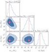 |
Fig. 1. Corner plot showing the posterior distributions of the key parameters estimated from the simulation (blue). The red lines represent the true values of the parameters injected into the simulation. The diagonal panels display the marginalized 1D posterior distributions for each parameter, while the off-diagonal panels show the 2D joint posterior distributions. |
3.2. Stochastic gravitational-wave background
We simulated cross-correlation measurements of the corresponding SGWB, assuming Tobs = 1 yr of integration with LVK with O5 sensitivity and a coherence time for the stochastic search of 4 seconds. This corresponds to frequency point estimates of the cross-correlation statistic evaluated every 0.25 Hz. We note that this choice differs from the value of 32 seconds that is typically used for current SGWB searches. We decided to reduce the coherence time in order to speed-up our hierarchical likelihood evaluation by a factor of 8. We also note that the choice of the length of the fast Fourier transform is not expected to strongly modify our results, as the sensitivity of detection of the SGWB is almost invariant for the choice of the coherence time (Thrane & Romano 2013) and mostly dependent on the observing time. As a detector baseline we use a five-detector LIGO (Hanford, Livingston, and India), Virgo and KAGRA networks at design sensitivities1 (Acernese et al. 2014; LIGO Scientific Collaboration 2015; Aso et al. 2013; Unnikrishnan 2013) and as a four-detector network the same but without LIGO India.
In Fig. 2, each data point is drawn from a Gaussian distribution centered on the true value of ΩGW(f), as calculated using Eq. (4), with a standard deviation, σ(f), given by Eq. (8). The uncertainty, σ(f), represents the sensitivity to an SGWB in every frequency bin. As argued before, σ(f) is directly related to the upper limits of the energy density of the SGWB, as fluctuation beyond this value is rare. This property allows us to detect the SGWB: if σ(f) is much larger than ΩGW(f), the variations in ΩGW(f) become effectively indistinguishable within the noise, making detection unlikely. Conversely, when σ(f) is sufficiently small, deviations in ΩGW(f) can be resolved, enabling us to identify the SGWB signal. Figure 2 also shows why low H0 values are easier to exclude with the SGWB. As we can observe, when we remove the 1/H02 dependence; namely, when we normalize the critical density of the Universe, ρc, the cross-correlation coefficients do not depend on H0 (as also indicated in Eq. 5), while the SGWB does. As a result, the S/N for the SGWB increases as 1/H0.
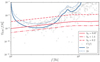 |
Fig. 2. Simulated SGWB cross-correlation spectrum, C(f) (points) with corresponding uncertainties, σ(f) (gray lines). The red lines are theoretical curves of ΩGW(f) for different h02, and the blue curves display the 1σ and 2σ sensitivity of the LVK at the design sensitivity (1 year of observation in O5). The scatter reflects realistic fluctuations centered on the true ΩGW(f). |
4. Results with simulated data
Using the simulated data described in Sect. 3 and the adopted prior ranges (see Table 1), we performed three separate analyses. The first considers only resolved CBC events (resolved CBCs), using two years of data. The second is a combined analysis (combined SGWB and CBCs), where we used one year of resolved BBH detections and one year of SGWB measurements. Finally, the third analysis focuses solely on one year of the SGWB to assess its sensitivity and, if possible, directly observe the impact of improvements due to unresolved sources.
Figure 3 displays the corner plot for the cosmological parameters H0 and Ωm with the redshift rate parameters. For a five-detector network, from the analysis using only resolved CBCs, we find  km s−1 Mpc−1 at 68% credible interval (CI). Combining SGWB information, we find
  km s−1 Mpc−1 at 68% CI, indicating no significant improvement in precision. This result indicates that most of the precision on H0 is determined by resolved spectral sirens. However, we note that the inclusion of the SGWB significantly helps in excluding the region of the parameter space that covers low values of H0 and Ωm. As also indicated by Cousins et al. (2025), this is a consequence of the fact that the S/N for the SGWB detection is higher for low values of H0 and Ωm. Instead, for a four-detector network, we find that the population posterior is entirely dominated by resolved sources and the inclusion of the SGWB is not able to improve the precision in any particular region of the H0, Ωm plane. We assumed that this result is also valid for the rest of the population parameters. As such, for the remainder of the paper, we focus on discussing possible constraints that can be achieved by the five-detector network as we are interested in discussing the impact of the SGWB.
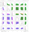 |
Fig. 3. Posterior distributions of the population parameters governing the cosmic expansion and the redshift evolution of the CBC merger rate. Results are shown for the resolved CBCs dataset (2 years of observations) using four detectors (orange) and five detectors (purple), and for the combined SGWB and CBCs dataset (1 year of individually resolved sources and 1 year of stochastic background) using four detectors (green) and five detectors (blue). Dashed red lines on the diagonal panels indicate injected (true) values. |
We observe that the datasets for individual sources and SGWB measure the rate parameter, R0, with similar precision. This is a consequence of the fact that the individual sources are mostly detected at lower redshifts and are the ones driving the inference on these population parameters. On γ we achieve an additional 10% precision with the combined analysis. We also see that the inclusion of the SGWB slightly introduces some preferences for the posteriors on zp and k. These two parameters govern the peak of the BBH merger rate and its redshift evolution for z > zp. The inclusion of the stochastic background makes possible the measurement  and helps to exclude low values of k; namely, we excluded models in which the rate increases beyond zp.
Figure 4 focuses on the mass model parameters and correlations with H0. The combined analysis does not lead to any improvement in these parameters, whereas the resolved-only analysis performs better.
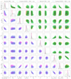 |
Fig. 4. Posterior distributions of the population parameters governing the cosmic expansion and the CBC mass distribution. Results are shown for the resolved CBCs dataset (2 years of observations) using four detectors (orange) and five detectors (purple), and for the combined SGWB and CBCs dataset (1 year of individually resolved sources and 1 year of stochastic background) using four detectors (green) and five detectors (blue). Dashed red lines on the diagonal panels indicate injected (true) values. |
To assess the performance of the inference, we produced posterior predictive checks (PPCs), which are defined as
 (19)
(19)
 (20)
(20)
where p(Φ|x) represents the posteriors on the population parameters and {x} the GW data that can either include or not the SGWB. By analyzing the PPCs for all three analyses in Fig. 5, we gain insight into the reconstructed redshift distribution (top panel), mass distribution (middle panel), and SGWB energy density (bottom panel), ΩGW(f). In Fig. 5 we report the PPCs for the analyses that we have performed. When considering resolved sources alone, the reconstructed redshift distribution is precise at low redshifts, while at higher redshifts z ≥ zp, the PPC is highly prior-dominated as we cannot determine the values of k and zp. When using the SGWB-only data, the reconstruction of the rate is strongly prior-dominated as there is too much degeneracy among the rate parameters R0, γ, and k, although there appears to be some information on the values of zp. Including individual sources and SGWB together provides a reconstruction of the rate informative up to redshift z = 2 − 3 consistent with what is observed in Callister et al. (2020). As we can see, by combining the resolved sources and the SGWB, the reconstruction of the BBH merger rate is less prior-dominated.
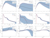 |
Fig. 5. PPCs for resolved CBC analysis (left), SGWB-only analysis (center), and the joint analysis of the two sources (right). The dashed and solid blue curves show the median and 90% credible bounds, and the red curve is the fiducial value injected. Top panel: Rate density R(z) of BBH mergers over the local merger rate, R0, as a function of redshift. Middle panel: Primary mass distribution as a function of the primary mass. Bottom panel: Posterior on ΩGWh02 as a function of the frequency. In all panels, the black line represents the 1σ curve. |
For the mass spectrum, we find that most of the information is collected from individual sources. In fact, for the SGWB-only analysis, the reconstruction of the mass spectrum is strongly prior dominated. The improvement in the precision of the reconstruction of SGWB energy density, when considering individual and SGWB sources, is mostly due to the improvement in the measure of γ and zp implied by the CBC rate parameters.
5. Reanalysis of GWTC-3
Using the approach defined in Sect. 2 and the likelihood in Eq. (1), we re-performed a population and cosmological spectral siren run with data from the latest public LVK observing run. We selected 59 BBHs detected during O3 with an inverse false alarm rate higher than 1 yr and used their posteriors released with GWTC-3 (Abbott et al. 2023d). To correct selection biases for the Poisson part of the likelihood, we used a set of injections in real O3 data2 released with Abbott et al. (2023c). For the stochastic data, we used the frequency point estimation of  and σ2(f) released3 with Abbott et al. (2021b). We only considered frequencies below 200 Hz to ease the computational load of the analysis. The
  that we used were evaluated every 0.03 Hz, corresponding to a coherence time for the SGWB search of 32 s and they were calculated with H0 = 67.9 km s−1 Mpc−1. For this analysis, we used the same BBH merger redshift model considered for the simulations. However, for the mass model we adopted a MULTI PEAK model, which can also describe a possible feature at masses of ∼10 M⊙. The MULTI PEAK model describes the mass distributions as
 (21)
(21)
 (22)
(22)
For the reanalysis of O3, we also made the implicit assumption that the likelihood in Eq. (1) is separable. For the O3 runs, this is a reasonable assumption as the removal of the individual sources of the population does not significantly modify the SGWB (Abbott et al. 2021b). The priors used for the analysis are reported in Table 1.
We performed two analyses, one considering only individual sources and the other also considering the SGWB upper limits. We find that the constraints on the population parameters, including also the cosmological parameters, are entirely given by the individual GW sources. In Fig. 6 we display the marginalized joint posterior distributions for these two analyses on the Hubble constant, Ωm and the parameter γ for the rate evolution. We find that the inclusion of the SGWB weakly helps in excluding low values of H0 and high values of γ from the 2σ CI areas. The posterior on the remaining of the population parameters is unchanged and we do not display it. In Fig. 7 we show the PPCs for the BBHs rate, mass distribution and SGWB reconstructed from the two analyses. We notice that the mass and rate reconstructions are equivalent in the case that the SGWB is included or not. We can also see that the reconstructed SGWB in both analyses is well below the 1σ upper limits from the stochastic searches. This means that the SGWB prediction is entirely given by the individual sources of CBCs and no additional information can be included from the SGWB likelihood. This is consistent with what was found in Callister et al. (2020).
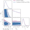 |
Fig. 6. Marginalized joint posterior distribution on the cosmological expansion parameters, and the rate parameter, γ, for an analysis including only 59 BBHs detected in O3 (purple line) and considering also the SGWB (blue line). The contour marks the 1σ and 2σ CIs. |
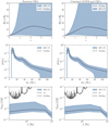 |
Fig. 7. PPCs for the resolved CBC analysis (left) and the joint analysis of the two sources (right). The dashed black and solid blue curves show the median and 90% credible bounds, and the red curve is the fiducial value injected. Top panel: Rate density, R(z), of BBH mergers over the local merger rate, R0, as a function of redshift. Middle panel: Primary mass distribution as a function of the primary mass. Bottom panel: Posterior on ΩGWh02 as a function of the frequency. In all the panels, the black line represents the 1σ curve. |
In parallel to this work, Cousins et al. (2025) present a spectral siren analysis using GWTC-3, including the SGWB. Although the results that we obtain are in excellent agreement, namely the inclusion of the SGWB does not modify significantly the inference on population and cosmological parameters, there are a few technical differences in our approach. From a data selection point of view, Cousins et al. (2025) used 42 BBH events with S/N > 11 observed in the first three LIGO and Virgo observations, while we used 59 BBHs detected during O3 with inverse false alarm rate higher than 1 per year. Another difference is that Cousins et al. (2025) used a PLP model to describe the masses, while we used a multi-peak model. From a data analysis perspective, Cousins et al. (2025) used as a prior on the population and cosmological parameters the posterior in Abbott et al. (2023b) from the spectral siren analysis. This was motivated by the separability of the likelihood in Eq. (1) that we also assume in our framework. Then the SGWB information is included as a likelihood term fitting posterior samples from Abbott et al. (2021b) on Ωα = 2/3, which is a quantity describing a SGWB as
 (23)
(23)
and corresponds to the SGWB expected by a population of BBHs emitting GWs during their inspiral phase at the 0 post-Newtonian order. Instead, we calculated ΩGW by re-weighting a GW energy spectrum that was calculated considering corrections for the GW emission up to the 3.5 post-Newtonian order (Ajith et al. 2008) and also for the merger and ring-down phases. However, we notice that our two approaches reach equivalent results because the SGWB is dominated in the 20 − 200 Hz region by the inspiral of BBH merger that can be safely estimated with the 0 post-Newtonian order emission; therefore, in that region, the SGWB is well approximated by the prescription in Eq. (23).
6. Conclusions
In this work we have discussed how it is possible to include the SGWB in spectral siren analyses for GW cosmology and enhance our understanding of astrophysical populations and cosmological parameters. Using simulated data at the design sensitivity of the LVK network’s O5 observing run, we applied a hierarchical Bayesian framework to infer a set of 14 hyperparameters, Φ, constraining key cosmological parameters such as H0 and Ωm, along with parameters governing the CBC mass distribution and the redshift evolution of the merger rate.
Our analysis that uses both four- and five-detector networks shows that combining SGWB data into the inference framework does not improve the precision on the marginal posteriors for cosmological parameters. In particular, we see that the Hubble constant estimates derived solely from resolved events yield  km s−1 Mpc−1 at 68% CI, while combining the SGWB information yields
  km s−1 Mpc−1 at 68% CI, indicating no significant improvement in precision. However, we find with the five-detector network that the inclusion of the SGWB helps exclude the lowest values of H0 and Ωm. Beyond cosmology, on an astrophysical population level, the integration of SGWB data slightly improves our understanding of the redshift evolution of CBC rates and helps with the measurements of γ and zp. The SGWB’s sensitivity to unresolved sources at higher redshifts allows for tighter constraints of the merger rate distribution at high redshifts.
When analyzing real O3 data, we find that the inclusion of the SGWB does not significantly improve any of the population or cosmological parameters. This result is consistent with the findings of Callister et al. (2020) and Abbott et al. (2021c) for population studies and Cousins et al. (2025) for the cosmological expansion parameters, and it is a consequence of the fact that the SGWB implied by individual sources is well below the sensitivity estimates for current stochastic searches.
Of course, in this exploratory study, we made a few simplistic assumptions that can be revised in follow-up studies. First, to preserve the separability of the likelihood in Eq. (1), we made the suboptimal choice of splitting the data into disjoint sets used for either the SGWB or individual source searches. This can be improved by developing a likelihood that takes additional correlations with the detected sources into account. In this sense, we believe that our improvement in the determination of the cosmological parameters is “conservative” as we are not using the full information present in the dataset. We expect that, with a joint likelihood for resolved sources and the SGWB, the precision on the cosmological parameters could be improved by including the stochastic. We also did not consider the possible contribution for the SGWB introduced by binary neutron stars and neutron star black hole binaries, which can be modeled with multi-population models.
Acknowledgments
We are grateful to M. Mancarella, A. Renzini and A. Toubiana for discussions during the development of this work. We are grateful to Cousins et al. (2025) and collaborators for the constructive feedback received during the internal LVK review of this work. This work received support from the French government under the France 2030 investment plan, as part of the Excellence Initiative of Aix Marseille University – amidex (AMX-19-IET-008 – IPhU). SM is supported by ERC Starting Grant No. 101163912–GravitySirens. This research made use of data, software and/or web tools obtained from the Gravitational Wave Open Science Center, a service of the LIGO Scientific Collaboration, the KAGRA Collaboration and the Virgo Collaboration. This material is based upon work supported by NSF’s LIGO Laboratory which is a majorfacility fully funded by the National Science Foundation. The authors are grateful for computational resources provided by the LIGO Laboratory (LHO) and supported by National Science Foundation Grants PHY-0757058 and PHY-0823459.
References
- Abbott, B. P., Abbott, R., Abbott, T. D., et al. 2017a, Phys. Rev. Lett., 119, 161101 [Google Scholar]
- Abbott, R., Abbott, T. D., Acernese, F., et al. 2017b, Nature, 551, 85 [NASA ADS] [CrossRef] [Google Scholar]
- Abbott, B. P., Abbott, R., Abbott, T. D., et al. 2017c, Phys. Rev. Lett., 119, 141101 [CrossRef] [Google Scholar]
- Abbott, B. P., Abbott, R., Abbott, T. D., et al. 2020, Liv. Rev. Relat., 23, 3 [NASA ADS] [Google Scholar]
- Abbott, B. P., Abbott, R., Abbott, T. D., et al. 2021a, ApJ, 909, 218 [NASA ADS] [CrossRef] [Google Scholar]
- Abbott, R., Abbott, T. D., Acernese, F., et al. 2021b, Phys. Rev. D, 104, 022004 [NASA ADS] [CrossRef] [Google Scholar]
- Abbott, R., Abbott, T. D., Abraham, S., et al. 2021c, ApJ, 913, L7 [NASA ADS] [CrossRef] [Google Scholar]
- Abbott, R., Abe, H., Acernese, F., et al. 2023a, ApJ, 949, 76 [NASA ADS] [CrossRef] [Google Scholar]
- Abbott, R., Abbott, T. D., Acernese, F., et al. 2023b, ApJ, 949, 76 [NASA ADS] [CrossRef] [Google Scholar]
- Abbott, R., Abbott, T. D., Acernese, F., et al. 2023c, Phys. Rev. X, 13, 011048 [NASA ADS] [Google Scholar]
- Abbott, R., Abbott, T. D., Acernese, F., et al. 2023d, Phys. Rev. X, 13, 041039 [Google Scholar]
- Acernese, F., Agathos, M., Agatsuma, K., et al. 2014, Class. Quant. Grav., 32, 024001 [Google Scholar]
- Ade, P. A. R., Aghanim, N., Arnaud, M., et al. 2016, A&A, 594, A13 [NASA ADS] [CrossRef] [EDP Sciences] [Google Scholar]
- Agarwal, A., Dupletsa, U., Leyde, K., et al. 2025, ApJ, 987, 47 [Google Scholar]
- Ajith, P., Babak, S., Chen, Y., Hewitson, M., & Krishnan, B. 2008, Phys. Rev. D, 77, 104017 [NASA ADS] [CrossRef] [Google Scholar]
- Allen, B., & Romano, J. D. 1999, Phys. Rev. D, 59, 102001 [NASA ADS] [CrossRef] [Google Scholar]
- Aso, Y., Michimura, Y., Somiya, K., et al. 2013, Phys. Rev. D, 88, 043007 [NASA ADS] [CrossRef] [Google Scholar]
- Bera, S., Rana, D., More, S., & Bose, S. 2020, ApJ, 902, 79 [NASA ADS] [CrossRef] [Google Scholar]
- Bom, C. R., Alfradique, V., Palmese, A., et al. 2024, MNRAS, 535, 961 [Google Scholar]
- Borhanian, S., & Sathyaprakash, B. 2024, Phys. Rev. D, 110, 083040 [Google Scholar]
- Callister, T., Fishbach, M., Holz, D. E., & Farr, W. M. 2020, ApJ, 896, L32 [NASA ADS] [CrossRef] [Google Scholar]
- Callister, T. A., Miller, S. J., Chatziioannou, K., & Farr, W. M. 2022, ApJ, 937, L13 [NASA ADS] [CrossRef] [Google Scholar]
- Christensen, N. 1992, Phys. Rev. D, 46, 5250 [NASA ADS] [CrossRef] [Google Scholar]
- Cigarrán Díaz, C., & Mukherjee, S. 2022, MNRAS, 511, 2782 [CrossRef] [Google Scholar]
- Cousins, B., Schumacher, K., Ka-Wai Chung, A., et al. 2025, ArXiv e-prints [arXiv:2503.01997] [Google Scholar]
- Di Valentino, E., Mena, O., Pan, S., et al. 2021, Class. Quant. Grav., 38, 153001 [NASA ADS] [CrossRef] [Google Scholar]
- Ezquiaga, J. M. 2021, Phys. Lett. B, 822, 136665 [NASA ADS] [CrossRef] [Google Scholar]
- Ezquiaga, J. M., & Holz, D. E. 2021, ApJ, 909, L23 [CrossRef] [Google Scholar]
- Ezquiaga, J. M., & Holz, D. E. 2022, Phys. Rev. Lett., 129, 061102 [NASA ADS] [CrossRef] [Google Scholar]
- Farah, A. M., Callister, T. A., Ezquiaga, J. M., Zevin, M., & Holz, D. E. 2025, ApJ, 978, 153 [Google Scholar]
- Farr, W. M., Fishbach, M., Ye, J., & Holz, D. E. 2019, ApJ, 883, L42 [NASA ADS] [CrossRef] [Google Scholar]
- Ferri, J., Tashiro, I. L., Abramo, L., et al. 2025, JCAP, 2025, 008 [Google Scholar]
- Finke, A., Foffa, S., Iacovelli, F., Maggiore, M., & Mancarella, M. 2021, JCAP, 2021, 026 [Google Scholar]
- Fishbach, M., Farr, W. M., & Holz, D. E. 2020, ApJ, 891, L31 [Google Scholar]
- Flanagan, E. E. 1993, Phys. Rev. D, 48, 2389 [Google Scholar]
- Ghosh, T., More, S., Bera, S., & Bose, S. 2025, Phys. Rev. D, 111, 063513 [Google Scholar]
- Gray, R., Hernandez, I. M., Qi, H., et al. 2020, Phys. Rev. D, 101, 122001 [NASA ADS] [CrossRef] [Google Scholar]
- Gray, R., Messenger, C., & Veitch, J. 2022, MNRAS, 512, 1127 [NASA ADS] [CrossRef] [Google Scholar]
- Gray, R., Beirnaert, F., Karathanasis, C., et al. 2023, JCAP, 2023, 023 [CrossRef] [Google Scholar]
- Holz, D. E., & Hughes, S. A. 2005, ApJ, 629, 15 [Google Scholar]
- Karathanasis, C., Mukherjee, S., & Mastrogiovanni, S. 2023, MNRAS, 523, 4539 [NASA ADS] [Google Scholar]
- Li, Y.-J., Tang, S.-P., Wang, Y.-Z., & Fan, Y.-Z. 2024, ApJ, 976, 153 [Google Scholar]
- Libanore, S., Artale, M. C., Karagiannis, D., et al. 2021, JCAP, 2021, 035 [CrossRef] [Google Scholar]
- LIGO Scientific Collaboration (Aasi, J., et al.) 2015, Class. Quant. Grav., 32, 074001 [Google Scholar]
- Madau, P., & Dickinson, M. 2014, ARA&A, 52, 415 [Google Scholar]
- Magaña Hernandez, I., & Ray, A. 2024, ArXiv e-prints [arXiv:2404.02522] [Google Scholar]
- Mali, U., & Essick, R. 2025, ApJ, 980, 85 [Google Scholar]
- Mancarella, M., Genoud-Prachex, E., & Maggiore, M. 2022, Phys. Rev. D, 105, 064030 [NASA ADS] [CrossRef] [Google Scholar]
- Mancarella, M., Iacovelli, F., Foffa, S., Muttoni, N., & Maggiore, M. 2024, Phys. Rev. Lett., 133, 261001 [Google Scholar]
- Mandel, I., Farr, W. M., & Gair, J. R. 2019, MNRAS, 486, 1086 [Google Scholar]
- Mastrogiovanni, S., Leyde, K., Karathanasis, C., et al. 2021, Phys. Rev. D, 104, 062009 [NASA ADS] [CrossRef] [Google Scholar]
- Mastrogiovanni, S., Laghi, D., Gray, R., et al. 2023, Phys. Rev. D, 108, 042002 [NASA ADS] [CrossRef] [Google Scholar]
- Mastrogiovanni, S., Pierra, G., Perriès, S., et al. 2024, A&A, 682, A167 [NASA ADS] [CrossRef] [EDP Sciences] [Google Scholar]
- Mukherjee, S. 2022, MNRAS, 515, 5495 [NASA ADS] [CrossRef] [Google Scholar]
- Mukherjee, S., Wandelt, B. D., Nissanke, S. M., & Silvestri, A. 2021, Phys. Rev. D, 103, 043520 [CrossRef] [Google Scholar]
- Mukherjee, S., Krolewski, A., Wandelt, B. D., & Silk, J. 2024, ApJ, 975, 189 [Google Scholar]
- Namikawa, T., Nishizawa, A., & Taruya, A. 2016a, Phys. Rev. Lett., 116, 121302 [Google Scholar]
- Namikawa, T., Nishizawa, A., & Taruya, A. 2016b, Phys. Rev. D, 94, 024013 [Google Scholar]
- Ng, K. K. Y., Vitale, S., Farr, W. M., & Rodriguez, C. L. 2021, ApJ, 913, L5 [NASA ADS] [CrossRef] [Google Scholar]
- Oguri, M. 2016, Phys. Rev. D, 93, 083511 [Google Scholar]
- Palmese, A., deVicente, J., Pereira, M. E. S., et al. 2020, ApJ, 900, L33 [Google Scholar]
- Palmese, A., Bom, C. R., Mucesh, S., & Hartley, W. G. 2023, ApJ, 943, 56 [NASA ADS] [CrossRef] [Google Scholar]
- Phinney, E. S. 2001, ArXiv e-prints [arXiv:astro-ph/0108028] [Google Scholar]
- Pierra, G., Mastrogiovanni, S., Perriès, S., & Mapelli, M. 2024, Phys. Rev. D, 109, 083504 [Google Scholar]
- Renzini, A. I., Romero-Rodríguez, A., Talbot, C., et al. 2023, ApJ, 952, 25 [Google Scholar]
- Romano, J. D., & Cornish, N. J. 2017, Liv. Rev. Relat., 20, 2 [CrossRef] [Google Scholar]
- Scelfo, G., Boco, L., Lapi, A., & Viel, M. 2020, JCAP, 2020, 045 [CrossRef] [Google Scholar]
- Schutz, B. F. 1986, Nature, 323, 310 [Google Scholar]
- Soares-Santos, M., Palmese, A., Hartley, W., et al. 2019, ApJ, 876, L7 [NASA ADS] [CrossRef] [Google Scholar]
- Talbot, C., & Golomb, J. 2023, MNRAS, 526, 3495 [NASA ADS] [CrossRef] [Google Scholar]
- Talbot, C., & Thrane, E. 2018, ApJ, 856, 173 [NASA ADS] [CrossRef] [Google Scholar]
- Taylor, S. R., Gair, J. R., & Mandel, I. 2012, Phys. Rev. D, 85, 023535 [Google Scholar]
- Thrane, E., & Romano, J. D. 2013, Phys. Rev. D, 88, 124032 [NASA ADS] [CrossRef] [Google Scholar]
- Tong, H., Fishbach, M., & Thrane, E. 2025, ApJ, 985, 220 [Google Scholar]
- Turbang, K., Lalleman, M., Callister, T. A., & van Remortel, N. 2024, ApJ, 967, 142 [NASA ADS] [CrossRef] [Google Scholar]
- Unnikrishnan, C. S. 2013, Int. J. Mod. Phys. D, 22, 1341010 [Google Scholar]
- van Remortel, N., Janssens, K., & Turbang, K. 2023, Progr. Part. Nucl. Phys., 128, 104003 [Google Scholar]
- Vitale, S., Gerosa, D., Farr, W. M., & Taylor, S. R. 2021, Inferring the Properties of a Population of Compact Binaries in Presence of Selection Effects (Singapore: Springer) [Google Scholar]
- Wei, J.-J., & Wu, X.-F. 2017, ApJ, 838, 160 [NASA ADS] [CrossRef] [Google Scholar]
- Yunes, N., & Siemens, X. 2013, Liv. Rev. Relat., 16, 9 [Google Scholar]
- Zazzera, S., Fonseca, J., Baker, T., & Clarkson, C. 2025, MNRAS, 537, 1912 [Google Scholar]
- Zhang, P. 2018, ArXiv e-prints [arXiv:1810.11915] [Google Scholar]
- Zhong, H., Reali, L., Zhou, B., Berti, E., & Mandic, V. 2025, ArXiv e-prints [arXiv:2501.17717] [Google Scholar]
Appendix A: Computation of hierarchical and stochastic likelihoods
We used the Python package ICAROGW to analyze our data. For a detailed explanation of its functionality, refer to Mastrogiovanni et al. (2024). Here, we provide a summary of the likelihood computation. The main application of ICAROGW is to infer the population parameters Φ that describe the production rate of events in terms of the GW parameters, θ, namely  . The hierarchical likelihood in Eq. 2, introduced in Sect. 2.1, models the probability of observing Nobs observations, each described by some parameters θ, in a dataset {x} over an observing time Tobs accounting for selection biases (Vitale et al. 2021). ICAROGW computes numerically the hierarchical likelihood in Eq. (2) as
![Mathematical equation: $$ \begin{aligned} \ln [\mathcal{L} (\{x\}|\Phi )]\approx -\frac{T_{\rm obs}}{N_{\rm gen}}\sum ^{N_{\rm det}}_{j = 1}s_j +\sum ^{N_{\rm obs}}_{i = 1} \ln \left[\frac{T_{\rm obs}}{N_{s,i}}\sum ^{N_{s,i}}_{j = 1}w_{i,j}\right], \end{aligned} $$](/articles/aa/full_html/2025/09/aa55124-25/aa55124-25-eq39.gif) (A.1)
(A.1)
where wi, j and sj are weights: wi, j has a dimension equal to the number of CBC mergers happening per unit of time and weights the sample, while sj weights the injections and it is defined with the dimension of a CBC merger rate per detector time. The first term derives from Monte Carlo integration to estimate
 (A.2)
(A.2)
where pdet(θ, Φ) is a detection probability or selection bias. Since an analytical form of pdet(θ, Φ) is typically unavailable, selection biases are evaluated using Monte Carlo simulations of injected and detected events (Abbott et al. 2021c). ICAROGW takes in input a set of Ndet detected injections out of Ngen total injections generated from a prior πinj(θ) to calculate the selection bias.
For each population model, ICAROGW calculates two numerical stability estimators. The first is the effective number of posterior samples per event:
 (A.3)
(A.3)
which ensures sufficient samples contribute to the integral, with a typical threshold of at least 20 effective samples per event (Callister et al. 2022; Talbot & Golomb 2023). The second is the effective number of injections:
![Mathematical equation: $$ \begin{aligned} N_{\rm eff, inj}=\frac{\left[\sum ^{N_{\rm det}}_{j = 1}s_j\right]^2}{\left[\sum ^{N_{\rm det}}_{j = 1}s^2_j -N_{\rm gen}^{-1}\left(\left[\sum ^{N_{\rm det}}_{j = 1}s_j\right]\right)^2\right]}, \end{aligned} $$](/articles/aa/full_html/2025/09/aa55124-25/aa55124-25-eq42.gif) (A.4)
(A.4)
where numerical stability typically requires Neff, inj > 4Nobs (Callister et al. 2022; Talbot & Golomb 2023).
The likelihood computation involves technical flags for configuration: nparallel = 2048, which is the number of posterior samples that will be used per event to compute wi, j, neffPE = −1, which indicates that there is no threshold for the effective number of posterior samples per event in Eq. A.3 and neffINJ=None, which is the effective number of injections required by the hierarchical likelihood. If neffINJ=None, a default threshold of NeffINJ = 4 × Nobs will be used.
We developed and implemented in ICAROGW a new function to calculate the SGWB likelihood, as described in Eq. 9, optimizing the computation of ΩGW. The expected ΩGW(f) calculation, conditioned on a set of hyperparameters, Φ, follows the form outlined in Eq. 4. This value depends on the average energy,  , radiated by individual binaries, which is expressed as
 (A.5)
(A.5)
where Φ denotes the intrinsic properties of a given binary (masses, redshift, etc.), p(Φ) is the distribution of these parameters across the CBC population, and this quantity is evaluated at the source-frame frequency fs = f(1 + z) in Eq. 4. The GW energy spectrum is calculated with functionalities from PYGWB Renzini et al. (2023) and Turbang et al. (2024) that calculated the GW energy spectrum up to the 3.5 post-Newtonian order for the GW emission and the merger and ring-down phase for non-precessing binaries.
Here, the integration spans the component masses m1 and m2. Extending this to include integration over redshift, the computation of the expected ΩGW(f) becomes a 3D integral. A practical alternative is to use Monte Carlo integration following the methodology used in Turbang et al. (2024), which estimates the integral by averaging over numerous samples drawn from the population.
In the implementation of this approach, we started by generating N random samples from uniform distributions for the parameters z, m1, and m2. Let the i-th sampled set of parameters be denoted as {zi, m1, i, m2, i}. For each of these samples, we calculated the energy spectrum, denoted as  . However, to evaluate ΩGW(f) for the population described by the hyperparameters Φ, re-weighting of these samples is necessary. The computation is expressed schematically as
 (A.6)
(A.6)
where wi are weights defined as
 (A.7)
(A.7)
Here, pdraw refers to the uniform distributions from which the initial samples were drawn, and the numerators represent the target distributions associated with the population characterized by Φ. This weighting allows us to compute ΩGW(f) while accounting for the desired population properties.
Appendix B: Measurement of the expansion rate, H(z)
To better understand the impact of combining resolved and unresolved sources on the reconstruction of the cosmic expansion history. We observe a modest improvement in the measurement of the expansion rate, H(z), when including the SGWB in the five-detector analysis, as shown on the left in Fig. B.1. This improvement is driven by the additional high-redshift information provided by unresolved sources, which is not accessible through individually resolved events alone. In particular, the SGWB contribution enables us to better constrain the high-redshift behavior of the expansion by disfavoring low values of both Ωm and H0, leading to a slightly tighter reconstruction of the expansion history. In contrast, the four-detector analysis, shown on the right, reveals no appreciable difference between the resolved-only and combineddatasets.
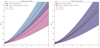 |
Fig. B.1. Posterior predictive distributions for the resolved CBCs dataset (purple) and the combined SGWB and CBCs dataset (blue) for results based on five (right) and four detectors (left). The solid black lines indicate the median predictions, with dashed lines showing the 90% CIs. The red curve denotes the injected (fiducial) model. |
All Tables
All Figures
|
Fig. 1. Corner plot showing the posterior distributions of the key parameters estimated from the simulation (blue). The red lines represent the true values of the parameters injected into the simulation. The diagonal panels display the marginalized 1D posterior distributions for each parameter, while the off-diagonal panels show the 2D joint posterior distributions. |
| In the text | |
|
Fig. 2. Simulated SGWB cross-correlation spectrum, C(f) (points) with corresponding uncertainties, σ(f) (gray lines). The red lines are theoretical curves of ΩGW(f) for different h02, and the blue curves display the 1σ and 2σ sensitivity of the LVK at the design sensitivity (1 year of observation in O5). The scatter reflects realistic fluctuations centered on the true ΩGW(f). |
| In the text | |
|
Fig. 3. Posterior distributions of the population parameters governing the cosmic expansion and the redshift evolution of the CBC merger rate. Results are shown for the resolved CBCs dataset (2 years of observations) using four detectors (orange) and five detectors (purple), and for the combined SGWB and CBCs dataset (1 year of individually resolved sources and 1 year of stochastic background) using four detectors (green) and five detectors (blue). Dashed red lines on the diagonal panels indicate injected (true) values. |
| In the text | |
|
Fig. 4. Posterior distributions of the population parameters governing the cosmic expansion and the CBC mass distribution. Results are shown for the resolved CBCs dataset (2 years of observations) using four detectors (orange) and five detectors (purple), and for the combined SGWB and CBCs dataset (1 year of individually resolved sources and 1 year of stochastic background) using four detectors (green) and five detectors (blue). Dashed red lines on the diagonal panels indicate injected (true) values. |
| In the text | |
|
Fig. 5. PPCs for resolved CBC analysis (left), SGWB-only analysis (center), and the joint analysis of the two sources (right). The dashed and solid blue curves show the median and 90% credible bounds, and the red curve is the fiducial value injected. Top panel: Rate density R(z) of BBH mergers over the local merger rate, R0, as a function of redshift. Middle panel: Primary mass distribution as a function of the primary mass. Bottom panel: Posterior on ΩGWh02 as a function of the frequency. In all panels, the black line represents the 1σ curve. |
| In the text | |
|
Fig. 6. Marginalized joint posterior distribution on the cosmological expansion parameters, and the rate parameter, γ, for an analysis including only 59 BBHs detected in O3 (purple line) and considering also the SGWB (blue line). The contour marks the 1σ and 2σ CIs. |
| In the text | |
|
Fig. 7. PPCs for the resolved CBC analysis (left) and the joint analysis of the two sources (right). The dashed black and solid blue curves show the median and 90% credible bounds, and the red curve is the fiducial value injected. Top panel: Rate density, R(z), of BBH mergers over the local merger rate, R0, as a function of redshift. Middle panel: Primary mass distribution as a function of the primary mass. Bottom panel: Posterior on ΩGWh02 as a function of the frequency. In all the panels, the black line represents the 1σ curve. |
| In the text | |
|
Fig. B.1. Posterior predictive distributions for the resolved CBCs dataset (purple) and the combined SGWB and CBCs dataset (blue) for results based on five (right) and four detectors (left). The solid black lines indicate the median predictions, with dashed lines showing the 90% CIs. The red curve denotes the injected (fiducial) model. |
| In the text | |
Current usage metrics show cumulative count of Article Views (full-text article views including HTML views, PDF and ePub downloads, according to the available data) and Abstracts Views on Vision4Press platform.
Data correspond to usage on the plateform after 2015. The current usage metrics is available 48-96 hours after online publication and is updated daily on week days.
Initial download of the metrics may take a while.