The New Generation Planetary Population Synthesis (NGPPS)

Di-Chang Chen; Christoph Mordasini; Alexandre Emsenhuber; Remo Burn; Ji-Wei Xie; Ji-Lin Zhou

doi:10.1051/0004-6361/202555380

Home

All issues

Volume 701 (September 2025)

A&A, 701 (2025) A94

Full HTML

Open Access

Issue		A&A Volume 701, September 2025


Article Number		A94
Number of page(s)		20
Section		Planets, planetary systems, and small bodies
DOI		https://doi.org/10.1051/0004-6361/202555380
Published online		05 September 2025

A&A, 701, A94 (2025)

VIII. Impact of host star metallicity on planet occurrence rates, orbital periods, eccentricities, and radius valley morphology

Di-Chang Chen¹^,2^,3^,4^★, Christoph Mordasini²^,5, Alexandre Emsenhuber², Remo Burn⁶, Ji-Wei Xie³^,4 and Ji-Lin Zhou³^,4

¹ School of Physics and Astronomy, Sun Yat-sen University, Zhuhai 519082, China
² Division of Space Research and Planetary Sciences, Physics Institute, University of Bern, Sidlerstrasse 5, 3012 Bern, Switzerland
³ School of Astronomy and Space Science, Nanjing University, Nanjing 210023, China
⁴ Key Laboratory of Modern Astronomy and Astrophysics, Ministry of Education, Nanjing 210023, China
⁵ Center for Space and Habitability, University of Bern, Gesellschaftsstrasse 6, 3012 Bern, Switzerland
⁶ Max-Planck-Institut für Astronomie, Königstuhl 17, Heidelberg 69117, Germany

^★ Corresponding author: chendch28@mail.sysu.edu.cn

Received: 4 May 2025
Accepted: 11 July 2025

Abstract

Context. The dust-to-gas ratio in the protoplanetary disc, which is likely imprinted into the host star metallicity, is a property that plays a crucial role during planet formation. On the observational side, statistical studies based on large exoplanet datasets have determined various correlations between planetary characteristics and host star metallicity.

Aims. We aim to constrain planet formation and evolution processes by statistically analysing planetary systems produced at different metallicities by a theoretical model, and we compare them with the correlations derived from observational samples.

Methods. We used the Generation III Bern model of planet formation and evolution to generate synthetic planetary systems at different metallicities. This global model incorporates the accretion of planetesimals and gas, planetary migration, N-body interactions between embryos, giant impacts, and protoplanetary disc evolution, as well as the planets’ long-term contraction and atmospheric loss of gaseous envelopes. Using synthetic planets biased to observational completeness, we analysed the impact of stellar metallicity on planet occurrence rates, orbital periods, eccentricities, and the morphology of the radius valley.

Results. Based on our nominal model, we find that (1) the occurrence rates of large giant planets and Neptune-sized planets are positively correlated with [Fe/H], while small sub-Earths exhibit an anti-correlation. In between, at radii of 1 to 3.5 R_⊕, the occurrence rate first increases and then decreases with increasing [Fe/H], with an inflection point at ~0.1 dex. (2) Planets with orbital periods shorter than ten days are more likely to be found around stars with a higher metallicity, and this tendency weakens with increasing planet radius. (3) Both giant planets and small planets exhibit a positive correlation between the eccentricity and [Fe/H], which could be explained by the self-excitation and perturbation of outer giant planets. (4) The radius valley deepens and becomes more prominent with increasing [Fe/H], accompanied by a lower super-Earth-to-sub-Neptune ratio. Furthermore, the average radius of the planets above the valley (2.1–6 R_⊕) increases with [Fe/H].

Conclusions. Our nominal model successfully reproduces many observed correlations with stellar metallicity either quantitatively or qualitatively, and supports the description of physical processes and parameters included in the Bern model. Quantitatively, the dependence of orbital eccentricity and period on [Fe/H] predicted by the synthetic population, however, is significantly weaker than observed. This discrepancy likely arises because the model only accounts for planetary interactions for the first 100 Myr and neglects the effects of the stellar environment (e.g. clusters, binaries). This suggests that long-term dynamical interactions between planets, along with the impact of binaries and/or companions, can drive the system towards a dynamically hotter state.

Key words: planets and satellites: general / planet–star interactions

© The Authors 2025

Open Access article, published by EDP Sciences, under the terms of the Creative Commons Attribution License (https://creativecommons.org/licenses/by/4.0), which permits unrestricted use, distribution, and reproduction in any medium, provided the original work is properly cited.

This article is published in open access under the Subscribe to Open model. Subscribe to A&A to support open access publication.

1 Introduction

The number of discovered exoplanets has exceeded 5500 through various surveys like High Accuracy Radial Velocity Planet Searcher (HARPS; Mayor et al. 2011), Lick (Fischer et al. 2014), Keck (Butler et al. 2017), CoRoT (Christian et al. 2006), Kepler (Borucki et al. 2010; Buchhave et al. 2018), and Transiting Exoplanet Survey Satellite (TESS; Ricker et al. 2015). Based on such a large observational dataset, numerous works have provided crucial constraints on the characteristics of exoplanetary systems (e.g. radius, occurrence rate, eccentricity, inclination, and orbital period ratio; Fabrycky et al. 2014; Fulton et al. 2017; Dawson & Johnson 2018; Zhu et al. 2018). Moreover, various correlations between the planetary characteristics and stellar properties (see the review by Zhu & Dong 2021) have been determined, which provide important insights into planet formation and evolution theory (Mulders 2018).

Of the various stellar properties, stellar metallicity is a crucial factor that has important impacts on planet formation. From theory, as a proxy for the dust-gas ratio of the protoplanetary disc, together with the disc mass, the metallicity determines the amount of solid materials in the disc and thus affects the planetary formation processes (Emsenhuber et al. 2021a), including the growth from dust to planetesimals (Ida & Makino 1993; Chambers 2001; Ormel & Klahr 2010), gas accretion (Pollack et al. 1996; Bodenheimer et al. 2000; Ayliffe & Bate 2012), and planet migration (Baruteau et al. 2014; Baruteau & Zhu 2016). From observations, the stellar metallicity is found to influence various planetary characteristics (e.g. occurrence rate, orbital architecture). For example, it has been well established that giant planets are preferentially hosted by metal-richer stars (Santos et al. 2001; Fischer & Valenti 2005; Wang & Fischer 2015; Chen et al. 2023). Some recent studies also show that the occurrence rate of smaller planets (especially in short-period orbits) may also be correlated with stellar metallicity (Wang & Fischer 2015; Moriarty & Ballard 2016; Dong et al. 2018; Zhu 2019). The orbital eccentricity is also found to be positively correlated with the stellar metallicity both for giant planets (Owen & Wu 2013; Buchhave et al. 2018) and small planets as found by the Kepler mission (Mills et al. 2019; An et al. 2023).

A powerful approach to constrain the key process of planetary formation and evolution is to perform planetary population synthesis (Ida & Lin 2004; Mordasini et al. 2009b; Liu et al. 2019; Burn & Mordasini 2024b; Pan et al. 2025) for statistical comparisons between the produced planetary systems of different metallicity from the theoretical model and the observed exoplanetary systems. This requires a global formation and evolution model (Mordasini et al. 2015; Raymond & Morbidelli 2022) that can predict the properties of planetary systems from different initial conditions (e.g. disc mass, dust-gas-ratio) that are representative of known protoplanetary discs. Furthermore, the detection bias of observational data should also be applied to the synthetic populations.

Here, we rely on the Generation III Bern model, a combined global end-end planetary formation and evolution model (Emsenhuber et al. 2021a), which was presented in the NGPPS I paper. By adopting the Bern model, we can generate synthetic planet populations that can predict various properties (e.g. mass, radii, and orbits) for planets of different sizes. In Emsenhuber et al. (2021b, NGPPS II), we used this model to perform the New Generation Planetary Population Synthesis of multi-planetary systems and discussed the initial conditions so that they can be representative of the protoplanetary disc population. For the detection biases, in Mishra et al. (2021, NGPPS VI), we introduce the KOBE program to simulate the geometrical limitations of the transit method and apply the detection biases and completeness of the Kepler survey. In Emsenhuber et al. (2025, NGPPS VII), we also show how to apply the detection biases of radial velocity method to the synthetic population. We have already performed analyses of the super Earth to cold Jupiter correlation (Schlecker et al. 2021, NGPPS III) and the architecture of multiple transiting planetary systems (Mishra et al. 2021, NGPPS VI) using the same synthetic population everywhere. Quantitative comparisons with various surveys (e.g. Kepler and HARPS) have also been performed (Mulders et al. 2019; Chen et al. 2024; Emsenhuber et al. 2025).

In this paper, we continue the NGPPS series and make statistical analyses as a function of stellar metallicities using the synthetic population of solar-like stars and compare with the observational results. The paper is organized as follows. In Sect. 2, we briefly introduce the coupled formation and evolution model. In Sect. 3, we describe how we set the initial conditions for our population synthesis. Then we investigate the correlations between the stellar metallicity and the planetary occurrence rates (Sect. 4), the radius valley morphology (Sect. 5), the orbital period (Sect. 6), and eccentricity (Sect. 7) and make quantitative comparisons with observations. Finally, we summarise the main results in Sect. 8.

2 Formation and evolution model

In this work, we used the Generation III Bern model of planetary formation and evolution, the latest generation of models first presented in Alibert et al. (2005). A full description of the Generation III model was given in Emsenhuber et al. (2021a); therefore we will provide here only a brief overview. The Bern model is a global model for the formation and evolution of planetary systems combining self-consistently descriptions for a significant number of physical processes.

The model begins with the formation stage. There, the evolution of the protoplanetary disc, the dynamical state of the planetesimal disc, concurrent solid and gas accretion by the protoplanets, gas-driven migration, and dynamical interactions between the protoplanets are tracked together.

The discs have a 1D radial, axis-symmetric representation. The evolution of the gas disc is computed by solving the advection-diffusion equation (Lüst 1952; Lynden-Bell & Pringle 1974) with the turbulent viscosity set following the standard α parametrization (Shakura & Sunyaev 1973). The gas disc’s vertical structure is computed following Nakamoto & Nakagawa (1994). Additional sink terms are included for the internal (Clarke et al. 2001) and external (Matsuyama et al. 2003) photoevaporation, plus accretion by the protoplanets. The planetesimal disc represents the solid component, with its dynamical state evolved following the balance between damping from the gas disc and stirring by the other planetesimals and the protoplanets (Rafikov 2004; Chambers 2006; Fortier et al. 2013).

Planet formation is assumed to occur by core accretion (Perri & Cameron 1974; Mizuno 1980). At the beginning, a given number of protoplanets with a mass of 10⁻² M_⊕ are inserted in the disc. The core grows by planetesimal accretion, which is taken to be in the oligarchic regime (Ida & Makino 1993; Thommes et al. 2003; Fortier et al. 2013). The planets are assumed to have an onion-like spherically symmetric structure with an iron core, a silicate mantle, a water ice layer and a gaseous envelope made of pure H/He. The internal structure of the planets (and thus their gas accretion rate, radius, luminosity, and interior structure) is calculated at all stages (attached, detached, evolution) by directly solving the 1D structure equations (Bodenheimer & Pollack 1986). For the composition of the planet core, we now use self-consistently the iron mass fraction as given by the disc compositional model according to Thiabaud et al. (2014); Marboeuf et al. (2014). This composition is tracked into the protoplanets when a protoplanet accretes planetesimals, and in giant impacts between protoplanets, yielding to a final iron to silicate ratio. For the gas envelope structure, at early times, gas accretion is limited by planet’s ability to radiate away the energy released by the accretion of both solid and gas. The efficiency of this process increases as the planet grows while the supply from the disc decreases as the disc depletes. Hence the gas accretion becomes limited by the supply from the disc at some point. When this occurs, the structure equations are used to determine the planet’s radius, allowing us to track the contraction and cooling (Bodenheimer et al. 2000).

The model also includes the Mercury N-body package (Chambers 1999) to track the dynamical interactions between the protoplanets. Gas-driven migration is included by means of additional forces in the N-body. We follow the prescription of Coleman & Nelson (2014) for Type I migration, and that of Dittkrist et al. (2014) for Type II migration. The transition between the two regimes is given by the criterion of Crida et al. (2006).

After a predetermined time of 100 Myr, the model switches to the evolution stage. Here, the model evolves each planet individually to 10 Gyr. The main aim is to track the thermodynamical evolution (cooling and contraction) of the planets following Mordasini et al. (2012). This stage also includes atmospheric escape (Jin et al. 2014; Jin & Mordasini 2018; Burn et al. 2024a), and tidal migration (Ferraz-Mello et al. 2008; Jackson et al. 2009; Benítez-Llambay et al. 2011). An important assumption, for planets whose mass is dominated by accreted solids, is how accreted volatile ices (mainly H₂O, CO₂, CH₄, CH₃OH, NH₃, but the model also allows for accretion of icy CO and N₂ in the very cold regions) are treated. Here, it is assumed that the mass which was accreted as ice evaporates and mixes perfectly with any hydrogen and helium which was accreted from the gas phase. Under this assumption, the mean molecular weight of the atmosphere increases, typically reducing the size of a H/He-rich planet but increasing the size for planets which would not contain H/He. To solve the internal structure of the mixed atmosphere, an equation of state (EOS) and opacities in the gaseous envelope are required. For both ingredients, a fully consistent treatment is challenging due to availability (EOS) or computational cost (opacity). Therefore, all volatile species are treated as H₂O for the EOS using AQUA (Haldemann et al. 2020) which is combined using the additive volume law with the EOS for H/He (Chabrier et al. 2019). Given the high temperatures of observable planets, water is typically in the gas phase and expected to be mixed well with H/He which holds even for the escaping material in the surface layer (see discussions in Burn et al. 2024a,b). For the opacity in the envelope, we assume a mixture of elements combining in chemical equilibrium to molecules assuming Solar abundances scaled with the overall metallicity (Freedman et al. 2014).

For photo-evaporative mass loss, the approach of Burn et al. (2024a) uses a mass-weighted average of the expected mass loss of H/He and pure H₂O following the works of Kubyshkina & Fossati (2021); Kubyshkina et al. (2018) and (Johnstone 2020) respectively. For H₂O, this approach relies on Energy-limited escape using a fitted efficiency while the H/He escape is directly taken from tables based on hydrodynamic models.

3 Population synthesis

A synthetic population of planetary systems is obtained by varying the initial conditions of the model. The procedure was described in Emsenhuber et al. (2021b). Here, we analysed data from the population with the internal identifier NG76Longshot. It is based on NG76 as presented in Emsenhuber et al. (2021b) but with prolonged N-body integration and modified assumptions for the long-term evolution (Burn et al. 2024a) as described in Sect. 2. The simulation was first analysed with a focus on the radius distribution and labelled the Mixed case in Burn et al. (2024a).

The starting point of the simulation mimics a disc in the state after the collapse of a cloud in the Class I stage. At this time zero, we assume here that pebbles have drifted and planetesimals and 100 larger, 0.01 M_⊕-mass embryos have formed. The latter are distributed randomly in the disc following a uniform distribution in logarithmic distance to the star. To generate a population of synthetic planets, we simulated 1000 systems with varied disc properties of young protoplanetary discs derived from observation: their initial gas mass (Tychoniec et al. 2018), metallicity, size (Andrews et al. 2010), inner edge (Venuti et al. 2017), and lifetime (distributed around 3 Myr by means of tuning the external photoevaporation rate). The initial solid mass of the disc is calculated by multiplying the mass of gas M_g and dust-to-gas-ratio f_D/G. For the f_D/G, we assume that stellar and disc metallicities are identical and thus, $\frac{f_{D / G}}{f_{D / G, \oplus}} = 10^{[F e / H]} .$ $\[\frac{f_{D / G}}{f_{D / G, \oplus}}=10^{[\mathrm{Fe} / \mathrm{H}]}.\]$ (1)

The dust-to-gas of the Sun f_D/G,⊕ is taken as 0.0149 (Lodders 2003). Figure 1 displays the distribution of [Fe/H] for our synthetic population. As can be seen, the range of [Fe/H] is restricted to −0.6 to 0.5, with a median value similar to the solar metallicity (black line). To compare with the observational sample, we selected planet host stars as single Sun-like stars from the LAMOST-Kepler-Gaia catalogue (Chen et al. 2021) with the following criteria: 4700K < T_eff < 6500K & log g > 4.0 & RUWE < 1.2. The median value and 1-σ range of [Fe/H] of the selected Kepler sample ( $- {0.01}_{- 0.21}^{+ 0.19}$ $\[-0.01_{-0.21}^{+0.19}\]$ ) are similar to those of the synthetic population ( $- {0.03}_{- 0.21}^{+ 0.23}$ $\[-0.03_{-0.21}^{+0.23}\]$ ). We also performed two-sample Kolmogorov-Smirnov (KS) and the resulted p–value is 0.0772, suggesting that the metallicities of the two samples show no significant difference. Other model parameters are kept constant across the systems, such as the turbulent viscosity parameter α = 2 × 10⁻³ or the planetesimal size R_plts = 300 m.

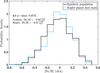Fig. 1

Probability density functions of the stellar metallicity ([Fe/H]) for the synthetic population (black) and Kepler Sun-like planet-host stars (cyan). In the top-left corner, we also print the KS p–value and the median values (1-σ interval) of the two samples.

4 Occurrence rate versus metallicity

The occurrence rate, i.e. the average number of planets per star, is one of the fundamental characteristics of exoplanet science. Determining how the occurrence rate depends on the properties of the host stars can provide crucial insights into the planet formation and evolution (Udry & Santos 2007; Zhu & Dong 2021). In this section, we divided the synthetic population into several bins according to their metallicities [Fe/H] and made quantitative analyses on the correlations between the occurrence rate of planets of different radii and the stellar [Fe/H].

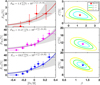Fig. 2

Left panels: the occurrence rate of hot Jupiters (top), warm Jupiters (middle), and cold Jupiters (bottom) as a function of stellar metallicity [Fe/H] from the synthetic NGPPS population and evolution model at 5 Gyr. The solid lines denote the best fits of Equation (1). For the occurrence rate, we were more concerned with the increasing trend rather than the absolute magnitude. Thus, to compare the synthetic results with observations, we used the fitted β derived from the observational sample in Chen et al. (2023) and the C derived from the synthetic sample to generate the 1 − σ intervals for the observational results, which are plotted as grey regions. Right panels: marginalized posterior probability density distributions of the parameters (C,β) for the occurrence rates of hot Jupiters (top), warm Jupiters (middle), and cold Jupiters (bottom) conditioned on the synthetic data generated by the Bern model.

4.1 Giant planets

We initialized our giant planetary sample from the synthetic planet population and select planets with masses between 0.1–13 Jupiter masses (M_J) as giant planets. According to previous studies (e.g. Dawson & Johnson 2018), we further divided the giant planetary sample into three categories according to their orbital periods:

P < 10 days, 12 hot Jupiters (HJs)
10 ≤ days ≤ P < 300 days, 130 warm Jupiter (WJs)
300 days ≤ P ≤ 3300 days, 154 cold Jupiter (CJs).

Here we set the typical time baselines (3300 days) for the observed time baseline for radius velocity (RV) surveys (e.g. the LCES HIRES/Keck Precision Radial Velocity Exoplanet Survey, the public HARPS RV database; Fúrész et al. 2008; Telting et al. 2014; Butler et al. 2017; Trifonov et al. 2020) as the upper limit of the period of cold Jupiters to facilitate subsequent comparison with observations.

To explore the correlation between stellar [Fe/H] and the occurrence rates of hot/warm/cold Jupiters, we divided the selected sample into several bins with equal numbers of stars according to their [Fe/H]. Then we counted the numbers of hot/warm/cold Jupiters and stars of each bins and obtained the occurrence rates $F = \frac{N_{p}}{N_{s}}$ $\[F=\frac{N_{\mathrm{p}}}{N_{\mathrm{s}}}\]$ for different [Fe/H]. To obtain the uncertainties of occurrence rates, we assumed that the numbers of giant planets and stars in each bin obey the Poisson distribution and resample for 1000 times. The uncertainty (1-σ interval) of [Fe/H] is set as the range of 50 ± 34.1 percentiles of given distribution in each bin. Figure 2 shows the occurrence rates of hot Jupiters F_HJ (top panel), warm Jupiters F_WJ (middle panel) and cold Jupiters F_CJ (bottom panel) as a function of stellar [Fe/H]. As can be seen, the occurrence rates of hot/warm/cold all seem to increase with stellar [Fe/H].

To quantify the above trends, referring to previous studies (e.g. Johnson et al. 2010), we fitted the occurrence rates as functions of metallicity with an exponential formula: $F ([F e / H], t) = C \times 10^{β [F e / H]} .$ $\[F([\mathrm{Fe} / \mathrm{H}], t)=C \times 10^{\beta[\mathrm{Fe} / \mathrm{H}]}.\]$ (2)

To obtain the values and uncertainties of C,β (hereafter, we denoted these coefficients as X for conciseness), we fitted them from the number of planets H drawn from a larger sample of T stars using Bayes’ theorem with the similar procedure as described in Sect. 4.2 of Johnson et al. (2010). Specifically, for a given set of X, the probability of star i with a planet is F([Fe/H]_i) and the probability of star j without of a planet is 1 − F([Fe/H]_j)). Thus, the probability/likelihood of forming H planets from T targets for a given X is $P \propto \prod_{i}^{H} (F ([F e / H]_{i}) \times \prod_{j}^{T - H} [1 - (F ([F e / H]_{j})] .$ $\[P \propto \prod_i^H(F([\mathrm{Fe} / \mathrm{H}]_i) \times \prod_j^{T-H}[1-(F([\mathrm{Fe} / \mathrm{H}]_j)].\]$ (3)

The marginalized log-likelihood is $\begin{aligned} \log L = & \sum_{i}^{H} \log (F ([F e / H]_{i})) \\ + \sum_{j}^{T - H} \log [1 - F ([F e / H]_{j})] . \end{aligned}$ $\[\begin{aligned}\log L= & \sum_i^H \log \left(F\left([\mathrm{Fe} / \mathrm{H}]_i\right)\right) \\& +\sum_j^{T-H} \log \left[1-F\left([\mathrm{Fe} / \mathrm{H}]_j\right)\right].\end{aligned}\]$ (4)

The best fits of X = [C, β] were set as where the maximum L conditioned on the simulated sample and the confidence intervals (1-σ: 68.3%, 2-σ: 95.4% and 3-σ: 99.7%) are estimated using a spline function.

In Fig. 2, we show the probability density functions of X for the hot Jupiters, warm Jupiters, and cold Jupiters in the top, middle, and bottom panels, respectively. As can be seen, all the occurrence rates of hot Jupiters, warm Jupiters, and cold Jupiters are positively correlated (β of ${1.3}_{- 0.6}^{+ 0.9}$ $\[1.3_{-0.6}^{+0.9}\]$ , ${1.3}_{- 0.2}^{+ 0.3}$ $\[1.3_{-0.2}^{+0.3}\]$ and ${1.3}_{- 0.1}^{+ 0.2}$ $\[1.3_{-0.1}^{+0.2}\]$ ) with the stellar metallicity with confidence levels (i.e. the probabilities for β > 0) of 96.76%, 99.99%, 99.99%, respectively. In order to further test the dependence of F_HJ, F_WJ and F_CJ on stellar [Fe/H], we also adopted a constant model (i.e. β = 0) model to fit the synthetic data. We calculated their Akaike information criterion (AIC). The resulting AIC differences between the best-fits of the constant model and exponential model are 6.6, 19.9, and 15.4 for F_HJ, F_WJ and F_CJ respectively, suggesting the exponential model is confidently preferred. The above analyses demonstrate that the occurrence rates of the synthetic giant planets are positively correlated with stellar metallicity.

The dependence of the occurrence rates of giant planets derived from the synthetic population are generally consistent with previous studies based on observational sample (e.g. Santos et al. 2001, 2004; Fischer & Valenti 2005; Johnson et al. 2010; Guo et al. 2017; Chen et al. 2023). Specifically, Johnson et al. (2010) and Chen et al. (2023) find that the occurrence rate of warm/cold Jupiters are positively correlated with stellar [Fe/H] as β ~ 1.2 based on RV and Kepler samples, which is in good agreement with our results within 1-σ uncertainties. Observational data also show that the occurrence rate of hot Jupiters exhibits a stronger dependence on [Fe/H] (Guo et al. 2017; Chen et al. 2023) and the derived β is ${1.6}_{- 0.3}^{+ 0.3}$ $\[1.6_{-0.3}^{+0.3}\]$ after removing the effect of temporal evolution (Chen et al. 2023), which is a bit larger (but statistically indistinguishable) comparing to β from the synthetic sample. One possible reason is that the synthetic sample does not include the ‘late-arrived’ hot Jupiters that migrated into the close proximity of their host stars long after their parent protoplanetary discs dissipated, which also makes contribution to the observed hot Jupiter populations (e.g.; Hamer & Schlaufman 2022; Chen et al. 2025). These ‘late-arrived’ hot Jupiters could be delivered via secular chaos in multiple giant planetary systems (Chen et al. 2025) and thus are expected to have a stronger metallicity dependence since metal-richer stars are more likely to form multiple giant planets (e.g. Dawson & Murray-Clay 2013; Petigura et al. 2018; Shibata et al. 2020; Yee & Winn 2023).

4.2 Neptune-sized planets

In this section, we selected planets with radii between ~3.5–6 R_⊕ as Neptune-sized planets from the synthetic population, yielding a sample of 273 Neptune-sized planets (16 hot, 152 warm, and 105 cold). We further divided the selected sample into several bins according to stellar [Fe/H] and obtained their occurrence rate. Figure 3 shows the occurrence rates of hot/warm/cold Neptune-size planets (F_HN, F_WN, and F_CN) as function of stellar [Fe/H]. Similar to Sect. 4.1, we performed the Bayesian analysis by modelling the planet occurrence rate with the exponential model (Equation 1). In the right panels, we show the probability density functions of the fitting parameters [C, β]. As can be seen, the occurrence rates of hot Neptunes, warm Neptunes and cold Neptunes are all positively correlated (β of ${0.5}_{- 0.5}^{+ 0.5}$ $\[0.5_{-0.5}^{+0.5}\]$ , ${0.8}_{- 0.2}^{+ 0.3}$ $\[0.8_{-0.2}^{+0.3}\]$ and ${0.6}_{- 0.3}^{+ 0.2}$ $\[0.6_{-0.3}^{+0.2}\]$ ) to the stellar metallicity with confidence levels (i.e. the probabilities for β > 0) ≳2–3σ. That is to say, Neptunesized planets tend to be hosted by metal-richer stars, though this preference is much weaker compared to that of giant planets.

The above results derived from the synthetic Neptune-sized planetary population are consistent with those derived from observational data. Specifically, based on the LAMOST-Kepler data, Dong et al. (2018) found that hot-Neptunes are preferentially hosted by metal-rich stars and their occurrence rates increase with stellar [Fe/H], which was then confirmed by Petigura et al. (2018) with the Keck spectra. By using the LAMOST-Gaia-Kepler kinematic catalogue (Chen et al. 2021), Chen et al. (2022) found that the fraction of Neptune-sized planets with orbital period in the range of 5–100 day increases with stellar [Fe/H] (β = ${0.8}_{- 0.4}^{+ 0.2}$ $\[0.8_{-0.4}^{+0.2}\]$ ; Chen et al. 2022). Recently, based on the homogeneous catalogue of stellar metallicities from Gaia Data Release 3, Vissapragada & Behmard (2025) found that hottest Neptunes tend to orbit metal-rich stars. Doyle et al. (2025) also reported an enhanced metallicity for our sample of Neptune desert planets from a homogeneous TESS sample with HARPS precise radial velocities, consistent with previous observational studies and our synthetic results.

4.3 Small planets (1–3.5 R_⊕)

In this section, we investigate the occurrence rate of small planets (i.e. radii within 1–3.5 R_⊕ and a period less than 400 days) as a function of stellar [Fe/H]. The synthetic population contains 2948 small planets in 850 systems. Referring to previous statistical studies on Kepler data (e.g. Zhu et al. 2018; Zhu 2019; Yang et al. 2020), we further decomposed the occurrence rate F into two factors: the fraction of stars hosting planetary systems η_system and the average number of Kepler planets in one system k.

With the similar procedure described in Sect. 4.1, we obtained F, η_system and k for different bins of different [Fe/H]. Then we fitted the correlation between F, η_system and k as a function of [Fe/H] with constant model and exponential model, and calculate their difference in AIC score ΔAIC ≡ AIC_Con − AIC_Exp. In the left panels of Fig. 4, we show the occurrence rate F as well as its two factors η_system and k as a function of stellar [Fe/H]. As shown in Fig. 4, when [Fe/H] ≲ 0.1 dex, the occurrence rate F as well as the two decomposed factor η_system and k increase with stellar [Fe/H] with ΔAIC of 8.4, 3.9 and 12.4, respectively. In contrast, when [Fe/H] ≳ 0.1 dex, F, η_system and k start to decline with ΔAIC of 10.5, 13.4 and 5.2, respectively. The trends of first increasing and then decreasing as well as the inflection point at ~0.1 dex are generally consistent with the observational results of Zhu (2019) derived from LAMOST-Kepler data.

We further divided the small planets into two subsamples: planets with radii ≥2 R_⊕ and <2 R_⊕. As shown in the middle panels of Fig. 4, F, η_system and k of planets with radii ≥2 R_⊕ rise continuously with increasing [Fe/H] (ΔAIC of 16.3, 13.3 and 7.6) when [Fe/H] ≲ 0.1 dex. We also note that F, η_system and k all seem to reach a plateau when [Fe/H] ≳ 0.1 dex. For planets with radii <2 R_⊕, the inflection point of [Fe/H] for F and η_system decreases to ~−0.1 dex. Besides, F and η_system decline significantly (ΔAIC of 9.2 and 12.2) when [Fe/H] ≳ −0.1 dex, while the average multiplicity k changes mildly (within 1-σ error bar) with [Fe/H]. That is to say, planets with radii ≥2 R_⊕ are more likely to be hosted by metal-rich stars comparing to planets with radii <2 R_⊕, which is consistent with previous statistical studies based on observation data (e.g. Chen et al. 2022).

One potential explanation for the decline of F at [Fe/H] ≳ 0.1 dex is that metal-richer stars host more giant planets and Neptunes. Their perturbation can drive dynamical instabilities (e.g. Zhou et al. 2007) and cause merge/ejection of small planets (e.g. Pu & Wu 2015; Lai & Pu 2017), reducing the number of planets or even the number of systems including small planets. To test whether this explanation is feasible, we excluded planetary systems with large planets with radii >3.5 R_⊕ (regardless of whether the period is more or less than 400 days) and divided the rest 624 planetary systems into eight bins with the same intervals of [Fe/H] as before. As shown in the bottom panels of Fig. 5, after eliminating the influence of large planets, the decrease of average multiplicity k at [Fe/H] ≳ 0.1 disappears for small planets as well as the two subsamples (with larger ΔAIC of 18.1, 17.6 and 12.1). Furthermore, the declines of F and η_system at super-solar metallicity disappear for the planets with radii ≥2 R_⊕ and become much weaker for those with radii <2 R_⊕. These changes are in good agreement with the prediction of the proposed explanation and thus support that the perturbation by larger planets is an important mechanism causing the decline of the occurrence rate at super-solar metallicity. Nevertheless, the decreasing of and F and η_system of planets with radii <2 R_⊕ at [Fe/H] ≳ 0.1 dex maintains, may indicating protoplanetary discs with super-solar metallicities have too many solids to form planets with radii <2 R_⊕.

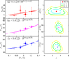Fig. 3

Left panels: the occurrence rate of hot Neptunes (top), warm Neptunes (middle), and cold Neptunes (bottom) as a function of stellar metallicity [Fe/H] from the synthetic NGPPS population by Bern planet formation and evolution model at 5 Gyr. The solid lines denote the best fits of Equation (1). Right panels: marginalized posterior probability density distributions of the parameters (C,β) for the occurrence rates of hot Neptunes (top), warm Neptunes (middle), and cold Neptunes (bottom) conditioned on the synthetic data generated by the Generation III Bern model.

4.4 Sub-Earths

Sub-Earths generally refer to planets smaller than our Earth, which are most difficult to detect due to the weakest signals. For observation, recently, Kepler data reveals an inflection in the occurrence rate of planets around ~1 R_⊕, suggesting that sub-Earths represent a unique population that is not an extension of super-Earths (Hsu et al. 2019; Neil & Rogers 2020; Qian & Wu 2021). However, the current sample of sub-Earth is not large enough to constrain their occurrence rate as a function of metallicity reliably.

Based on the synthetic population generated by the Bern model, we obtained a sample of 635 sub-Earths with radii between 0.3–1 R_⊕ and orbital period ≤400 days. investigate the correlations between their occurrence rate and stellar [Fe/H]. We divided the stellar sample into eight bins according to [Fe/H] and obtain the occurrence rate F, the fraction of stars hosting sub-Earths η_system and the average multiplicity k of sub-Earths for different bins of different [Fe/H]. Figure 6 shows the evolution of F, η_system and k with stellar [Fe/H] for sub-Earths. As can be seen, F as well as η_system and k of the sub-Earths all decrease significantly with increasing [Fe/H]. To quantify the above trends, we made fitting and analyses with the same procedure described in Sect. 4.1. The best-fits of preferred models are plotted as solid lines in Fig. 6. The exponential models are preferred for F, η and k of sub-Earths compared to the constant model with ΔAIC of 33.7, 26.4 and 15.3, respectively. F, η and k are negatively correlated with stellar [Fe/H] with confidence levels (i.e. β < 0) of 99.99%, 99.98% and 95.09%, respectively. The above analyses suggest that sub-Earths tend to be hosted by metal-poor stars with confidence level ≳2–3σ. This result is expected because around metal-rich stars the amount of silicates/Fe is more likely to be sufficiently high that planets that are larger than sub-Earths are preferentially formed.

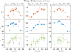Fig. 4

Occurrence rate, F, the fraction of stars hosting planetary system, η_system, and the average multiplicity, k, as a function of stellar metallicity [Fe/H] for Kepler-like planets (R_p: 1–4R_⊕, P < 400 d, left panels), planets with radii between 2–4 R_⊕ (middle panels), and planets with radii between 1–2 R_⊕ (right panels) from the synthetic population by Bern planet formation and evolution model at 5 Gyr. In the left panels, we also plot the observational results derived from Kepler data (Zhu 2019) as grey points and error bars. As mentioned before, we were more concerned with trends and thus we renormalized the amplitude of observed occurrence rate tracer of Kepler systems with planets into the average synthetic η_system.

5 Radius valley morphology as functions of stellar metallicity

One of the most interesting discoveries in exoplanet science in recent years is the radius valley, a dip at ~1.9 R_⊕ in the radius distribution as revealed by high-precision sample from Kepler (e.g. Fulton et al. 2017; Van Eylen et al. 2018). Plenty of previous statistical studies have explored the dependence of the radius valley on planetary and stellar properties, providing crucial insights into the origin of the radius valley (e.g. Fulton et al. 2017; Van Eylen et al. 2018; Owen & Murray-Clay 2018; Berger et al. 2020; Chen et al. 2022). The radius valley had been theoretically predicted to exist (Owen & Wu 2013; Lopez & Fortney 2013; Jin et al. 2014) before it was discovered in the observational data. In a previous paper (Burn et al. 2024a), we find that the synthetic NG76Longshot population can reproduce the radius distributions with a similar position of the valley centre ~1.9 R_⊕ (e.g. Owen & Wu 2013, 2017; Fulton et al. 2017), the radius cliff at ~3 R_⊕ (e.g. Kite et al. 2019) and the anti-correlation on orbital period (Van Eylen et al. 2018; Martinez et al. 2019) revealed from observational data. In this subsection, we further investigate the morphology of the radius valley as a function of stellar metallicity quantitatively. This is an interesting theoretical prediction that should be tested with observational data.

We initialized our planetary sample from the synthetic planetary population at 2 Gyr (the typical age of planetary sample of Chen et al. (2022) after controlling parameters) and select planets close to the radius valley (i.e. radius between 1–6 R_⊕) with orbital period between 1–100 days. To apply the detection biases, we simulated the Kepler mission completeness using the Kepler Observes Bern Exoplanets (KOBE) program (Mishra et al. 2021). Furthermore, we also excluded planets with detection efficiency less than 50% since most of Kepler planets in Chen et al. (2022) lie above the 50% detection efficiency limit (see Fig. B3 of their paper). Figure 7 displays the planetary radius-period diagram and planetary radius histogram. As can be seen, the synthetic sample shows an obvious bimodal radius distribution (with p–value <0.003 from maximizes Hartigan’s dip statistic).

The radius valley are found to be located at $R_{p 0}^{Valley} \sim 1.9 \pm 0.2 R_{\oplus}$ $\[R_{\mathrm{p} 0}^{\text {Valley }} \sim 1.9 \pm 0.2 ~R_{\oplus}\]$ (e.g. Owen & Wu 2017; Fulton et al. 2017; Jin & Mordasini 2018) and to be dependent on stellar mass M_* (Berger et al. 2020) and planetary orbital period P (Van Eylen et al. 2018), which can be characterized as $R_{p}^{valley} = R_{p 0}^{valley} {(\frac{M_{*}}{M_{⊙}})}^{h} {(\frac{P}{10 days})}^{g},$ $\[R_{\mathrm{p}}^{\text {valley }}=R_{\mathrm{p} 0}^{\text {valley }}\left(\frac{M_*}{M_{\odot}}\right)^h\left(\frac{P}{10 \text { days }}\right)^g,\]$ (5)

where h and g are are the corresponding slopes, which are adopted as ${0.21}_{- 0.07}^{+ 0.06}$ $\[0.21_{-0.07}^{+0.06}\]$ and $- {0.09}_{- 0.03}^{+ 0.02}$ $\[-0.09_{-0.03}^{+0.02}\]$ (Ho & Van Eylen 2023; Ho et al. 2024), respectively. For our synthetic sample, M_* = 1 M_⊙ and thus the upper and lower boundaries of radius valley are set as $R_{upper}^{Valley} = 2.1 R_{\oplus} {(\frac{P}{10 days})}^{- 0.09}$ $\[R_{\text {upper }}^{\text {Valley }}=2.1 ~R_{\oplus}\left(\frac{P}{10 \text {days }}\right)^{-0.09}\]$ and $R_{lower}^{Valley} = 1.7 R_{\oplus} {(\frac{P}{10 days})}^{- 0.09}$ $\[R_{\text {lower }}^{\text {Valley }}=1.7 ~R_{\oplus}\left(\frac{P}{10 \text {days}}\right)^{-0.09}\]$ , respectively. Thus, we divided the planetary sample into four subsamples according to their radius as follows:

Valley planet (VP): $R_{lower}^{Valley} \leq R_{p} \leq R_{upper}^{Valley}$ $\[R_{\text {lower }}^{\text {Valley}} \leq R_{\mathrm{p}} \leq R_{\text {upper }}^{\text {Valley}}\]$ ;
Super-Earth (SE): $1 R_{\oplus} \leq R_{p} < R_{lower}^{Valley}$ $\[1 ~R_{\oplus} \leq R_{\mathrm{p}}<R_{\text {lower}}^{\text {Valley}}\]$ ;
Sub-Neptune (SN): $R_{upper}^{Valley} < R_{p} \leq 3.5 R_{\oplus}$ $\[R_{\text {upper}}^{\text {Valley}}<R_{\mathrm{p}} \leq 3.5 ~R_{\oplus}\]$ ;
Neptune-sized planet (NP): 3.5 R_⊕ < R_p ≤ 6 R_⊕.

Moreover, using the composition data provided by the synthetic population, the planetary sample can be classified into three categories: pure rocky planets (silicate+Fe) with no envelope, planets with water-rich envelope (mass fraction of water in the envelope ≥0.9), and planets with H/He-rich envelope (mass fraction of water <0.9). As can be seen in Fig. 7, for the synthetic sample, Neptune-like planets all have H/He-rich envelopes. Super-Earths are mostly purely rocky which mainly (~75%) formed in-situ by a giant impact stage (Class I system architecture and formation pathway in the classification of Emsenhuber et al. 2023) or lost their gaseous envelope completely (more relevant at short orbits and larger super-Earths), while sub-Neptunes are mainly water-rich planets that formed ex-situ and migrated substantially to their present-day location (Class II in Emsenhuber et al. 2023).

To investigate the morphology of radius valley as a function of stellar metallicity, we divided the planetary sample into eight bins with same size according to [Fe/H]. Figures 8 and 9 display the radius-period diagrams and radius histograms for planets with different metallicities. As can be seen, with the decrease of [Fe/H], the radius valley becomes less prominent. Also, the number (fraction) of super-Earths grows, while the numbers (fractions) of sub-Neptunes and Neptune-like planets decline. Moreover, the radii of sub-Neptunes seem to shrink with decreasing [Fe/H]. Very interestingly, such trends are consistent with the observational results derived from the CKS sample (Owen & Murray-Clay 2018) and LAMOST-Gaia-Kepler sample (Chen et al. 2022).

To evaluate the above trends quantitatively, we adopted the five morphology metrics of radius valley defined in Chen et al. (2022), which are described as follows:

The contrast of radius valley C_valley, defined as the number ratio of super-Earths (N_SE) plus sub-Neptunes (N_SN) to the valley planets (N_VP), i.e. $C_{v a l l e y} = \frac{N_{S E} + N_{S N}}{N_{V P}} .$ $\[C_{\mathrm{valley}}=\frac{N_{\mathrm{SE}}+N_{\mathrm{SN}}}{N_{\mathrm{VP}}}.\]$ (6)
The asymmetry on the two sides of the valley defined as the number ratio (in logarithm) of super-Earths to sub-Neptunes, i.e. $A_{valley} = \log_{10} (\frac{N_{S E}}{N_{S N}}) .$ $\[A_{\text {valley }}=\log _{10}\left(\frac{N_{\mathrm{SE}}}{N_{\mathrm{SN}}}\right).\]$ (7)
The average radius of planets with size larger than Valley planets, i.e. $R_{v a l l e y}^{+} = \frac{1}{N_{S N} + N_{N P}} \sum_{i}^{N_{S N} + N_{N P}} R_{i},$ $\[R_{\mathrm{valley}}^{+}=\frac{1}{N_{\mathrm{SN}}+N_{\mathrm{NP}}} \sum_i^{N_{\mathrm{SN}}+N_{\mathrm{NP}}} R_{\mathrm{i}} \text {, }\]$ (8)

where $R_{upper}^{Valley} < R_{i} < 6 R_{\oplus}$ $\[R_{\text {upper}}^{\text {Valley}}<R_{\mathrm{i}}<6 ~R_{\oplus}\]$ .
The average radius of planets with size smaller than Valley planets, i.e. $R_{valley}^{-} = \frac{1}{N_{S E}} \sum_{i}^{N_{S E}} R_{i},$ $\[R_{\text {valley }}^{-}=\frac{1}{N_{\mathrm{SE}}} \sum_i^{N_{\mathrm{SE}}} R_{\mathrm{i}},\]$ (9)

where $1.0 R_{\oplus} < R_{i} < R_{lower}^{Valley}$ $\[1.0 ~R_{\oplus}<R_{\mathrm{i}}<R_{\text {lower}}^{\text {Valley}}\]$ .
The number fraction of Neptune-sized planets in the whole planet sample, i.e. $f_{N P} = \frac{N_{N P}}{N_{S E} + N_{V P} + N_{S N} + N_{N P}} .$ $\[f_{\mathrm{NP}}=\frac{N_{\mathrm{NP}}}{N_{\mathrm{SE}}+N_{\mathrm{VP}}+N_{\mathrm{SN}}+N_{\mathrm{NP}}}.\]$ (10)

Then we calculated these metrics for the eight bins of different [Fe/H] (as shown in Fig. 10). The uncertainties of C_valley, A_valley and f_NP were derived using error propagation based on the Poisson errors in the planet numbers. The uncertainties of $R_{valley}^{+}$ $\[R_{\text {valley}}^{+}\]$ and $R_{valley}^{-}$ $\[R_{\text {valley }}^{-}\]$ were calculated using a bootstrapping method.

We also fitted the data points using two models (i.e. constant model and linear model) and evaluated these two models by calculating the difference in AIC score (ΔAIC). The fitting results are as follows:

For C_valley, the linear increasing model is preferred over the constant model with ΔAIC = 11.7.

The best fit is $C_{valley} = {15.9}_{- 4.6}^{+ 3.4} \times [F e / H] + {7.0}_{- 1.1}^{+ 1.6} .$ $\[C_{\text {valley }}=15.9_{-4.6}^{+3.4} \times[\mathrm{Fe} / \mathrm{H}]+7.0_{-1.1}^{+1.6}.\]$ (11)
For A_valley, the linear decay model is preferred over the constant model with ΔAIC = 17.9.

The best fit is $A_{valley} = - {1.0}_{- 0.2}^{+ 0.2} \times [F e / H] + {0.12}_{- 0.01}^{+ 0.01} .$ $\[A_{\text {valley }}=-1.0_{-0.2}^{+0.2} \times[\mathrm{Fe} / \mathrm{H}]+0.12_{-0.01}^{+0.01}.\]$ (12)
For $R_{valley}^{+}$ $\[R_{\text {valley}}^{+}\]$ , the linear increasing model is preferred over the constant model with ΔAIC = 10.5.

The best fit is $\log_{10} (\frac{R_{valley}^{+}}{R_{\oplus}}) = {0.06}_{- 0.02}^{+ 0.02} \times [F e / H] + {0.45}_{- 0.02}^{+ 0.03} .$ $\[\log _{10}\left(\frac{R_{\text {valley }}^{+}}{R_{\oplus}}\right)=0.06_{-0.02}^{+0.02} \times[\mathrm{Fe} / \mathrm{H}]+0.45_{-0.02}^{+0.03}.\]$ (13)
For $R_{valley}^{-}$ $\[R_{\text {valley }}^{-}\]$ , the fitting linear index (0.03 ± 0.04) is consistent with zero within 1-σ, suggesting that $R_{valley}^{-}$ $\[R_{\text {valley }}^{-}\]$ shows no dependence on [Fe/H]. The best fit is $R_{valley}^{-} = {1.35}_{- 0.02}^{+ 0.02} R_{\oplus} .$ $\[R_{\text {valley }}^{-}=1.35_{-0.02}^{+0.02} ~R_{\oplus}.\]$ (14)
For f_NP, the linear increasing model is preferred over the constant model with ΔAIC = 45.6. The best fit is $f_{N P} = {0.15}_{- 0.04}^{+ 0.04} \times [F e / H] + {0.05}_{- 0.01}^{+ 0.02} .$ $\[f_{\mathrm{NP}}=0.15_{-0.04}^{+0.04} \times[\mathrm{Fe} / \mathrm{H}]+0.05_{-0.01}^{+0.02}.\]$ (15)

The fitting results of simulation data confirm the apparent trends seen in Fig. 10 and suggest that the radius valley deepens with increasing [Fe/H]. Furthermore, metal-rich stars host more (and larger) sub-Neptunes and Neptune-sized planets.

Such trends are expected. As shown in Equation (1), protoplanetary discs with higher [Fe/H] exhibit higher solid surface densities. Consequently, as [Fe/H] increases, the planets grow faster and attain larger masses. More planets can reach the mass required for significant inward migration before the disc dissipates (Emsenhuber et al. 2023), leading to higher occurrence rates of Neptunes (f_NP) and sub-Neptunes in the inner systems. Moreover, massive planets have deeper gravitational potentials, allowing them to retain more of their envelopes after photo-evaporation and have larger radii ( $R_{valley}^{+}$ $\[R_{\text {valley}}^{+}\]$ ), as the mass-loss rate follows $\dot{M} / M \propto R^{3} / M^{2} ≃ 1 / M$ $\[\dot{M} / M \propto R^{3} / M^{2} \simeq 1 / M\]$ under energy-limited escape (Mordasini 2020). In contrast, super-Earths are mainly rocky planets that formed in-situ, with lower requirements for formation speed and mass. As a result, the occurrence rate and average size of super-Earths ( $R_{valley}^{-}$ $\[R_{\text {valley }}^{-}\]$ ) show no significant dependence on [Fe/H]. This also explains why A_valley exhibits a positive trend, driven by the increased occurrence of sub-Neptunes rather than a decrease in super-Earths (see also the right panels of Fig. 4). For C_valley, as shown in Fig. 11, the lowest-mass water-rich planets fill the valley in radius space at low [Fe/H], explaining the increasing trend of C_valley with [Fe/H]. To explain this, it is insightful to remember that on a distance-mass diagram, inward motion occurs if the migration rate is shorter than the solid accretion rate (gas accretion is not efficient at this mass range yet). Thus, for low [Fe/H] and reduced accretion, orbital migration occurs at lower planet mass, which allows for low-mass water-worlds to reach the inner regions of the system. The outcome is similar to that around low-mass stars where less solid material is available due to discs that were less-massive than expected (Luque & Pallé 2022; Burn et al. 2024b; Venturini et al. 2024).

In Fig. 10, we also plot the best-fits and 1-σ intervals of the observational results derived from the LAMOST-Gaia-Kepler sample (Chen et al. 2022) as dashed black lines and grey regions. As can be seen, for all five metrics, the trends with [Fe/H] in the synthetic population are quantitatively consistent with those of Chen et al. (2022) within ~1–2σ error bars, demonstrating that the synthetic population can reproduce very well the observed dependence of the radius valley morphology on host star metallicity. This quantitative, and not merely qualitative excellent match is a non-trivial result as the model was not optimized or otherwise conditioned to reproduce these observations. In contrast, the entire formation and evolution that leads to this outcome is governed by the physical processes included in the model.

Fig. 5

Similar to Fig. 4 but excluding planetary systems including planets with radii >3.5 R_⊕.

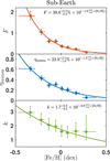Fig. 6

Occurrence rate, F (top), the fraction of stars that host planetary system, η_system (middle), and the average multiplicity, k (bottom) as a function of stellar metallicity [Fe/H] for the sub-Earths from the synthetic population by Bern planet formation and evolution model at 5 Gyr.

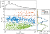Fig. 7

Period–radius diagram of planets selected from the synthetic population at 2 Gyr after applying the detection selection similar to PAST III (Chen et al. 2022). Planets with different compositions are plotted in different colours: red for H/He-rich envelopes, blue for waterrich envelopes, and green for purely rocky (Silicate+Fe) planets. The dashed lines represent the boundaries of planet radii between different subsamples: Neptune-sized planets, sub-Neptune, valley planet, and super-Earth. Histograms of planetary radius and orbital period are shown in the right panel and the top panel, respectively.

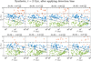Fig. 8

Orbital period-radius diagram of planets with different metallicity [Fe/H] from the synthetic population at 2 Gyr after applying the detection bias similar to PAST III.

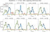Fig. 9

Radius distribution of planets with different metallicity [Fe/H] from the synthetic population after applying a detection selection similar to PAST III.

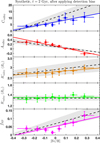Fig. 10

Five metrics to characterize the radius valley morphology (i.e. $C_{valley}, A_{valley}, R_{valley}^{+}, R_{valley}^{-}$ $\[C_{\text {valley }}, A_{\text {valley }}, R_{\text {valley }}^{+}, R_{\text {valley }}^{-}\]$ , and f_NP) as functions of [Fe/H] for synthetic population at 2 Gyr after applying the detection bias. The solid lines denote the best fits derived from the synthetic population. The best fits and 1-σ interval derived from the selected observational sample of LAMOST–Gaia–Kepler catalogue (Chen et al. 2021, 2022) are plotted as dashed black lines and grey regions.

6 The distributions of planets as a function of orbital periods

In this section, again using the synthetic NG76Longshot population generated by the Bern model, we explore how the planet population depends on host star metallicity as a function of orbital periods. We initialized the planetary sample based on the synthetic population at 5 Gyr and selected planets with an orbital period ≤400 days.

Figure 12 displays the metallicities of planet host stars as a function of the orbital period. To evaluate the correlation between the metallicity and orbital periods, we first adopted the Pearson test and the resulted Pearson coefficient is -0.06 with a p–value of 1.5 × 10⁻⁴ that the two properties are uncorrelated. We also performed the KS test between the metallicity of stars that host planets with periods more and less than ten days. The resulting p–value is 0.015, suggesting that the two subsamples are not drawn from the same distribution. The above tests demonstrate that the metallicity and orbital periods have a weak but statistically significant anti-correlation, with highest average [Fe/H] at a small distance. Referring to Mulders et al. (2016), we also calculated the kernel regression of the mean metallicity of planet population at an orbital period P with the following formula: $\bar{[F e / H]} (P) = \frac{\sum_{i = 0}^{n} [F e / H]_{i} f_{o c c, i} K (\log (P / P_{i}), σ)}{\sum_{i = 0}^{n} f_{o c c, i} K (\log (P / P_{i}), σ)},$ $\[\overline{[\mathrm{Fe} / \mathrm{H}]}(P)=\frac{\sum_{i=0}^n~[\mathrm{Fe} / \mathrm{H}]_i f_{\mathrm{occ}, i} K\left(\log \left(P / P_i\right), \sigma\right)}{\sum_{i=0}^n f_{o c c, i} K\left(\log \left(P / P_i\right), \sigma\right)},\]$ (16)

where [Fe/H]_i and P_i are the metallicity and orbital period for each planet in the synthetic sample. f_occ is the ratio of the number of planets over the number of stars where planets are detectable, multiplied by the geometric transit probability, which is used to eliminate the effect of detection bias. We set f_occ = 1 as the synthetic population aim to reveal the intrinsic planet distribution. Here we adopted the same log-normal kernel with σ = 0.29 as Mulders et al. (2016): $K (\log P, σ) = \frac{1}{\sqrt{2 π}} e^{- 0.5 (\log P / σ)^{2}} .$ $\[K(\log P, \sigma)=\frac{1}{\sqrt{2 \pi}} e^{-0.5(\log P / \sigma)^2}.\]$ (17)

The uncertainties of $\bar{[F e / H]}$ $\[\overline{[\mathrm{Fe} / \mathrm{H}]}\]$ are calculated using a bootstrapping method. As shown in Fig. 12, the mean metallicity (solid red line) and 1-σ interval (red region) generally decreases with the increase of orbital periods. We then calculated the mean average metallicities for planet populations with orbital periods more or less than ten days using Eq. (16) and their difference, $Δ [F e / H] = \bar{[F e / H]} (P < 10 days) - \bar{[F e / H]} (P > 10 days)$ $\[\Delta[\mathrm{Fe} / \mathrm{H}]=\overline{[\mathrm{Fe} / \mathrm{H}]}(\mathrm{P}<10 \text { days })-\overline{[\mathrm{Fe} / \mathrm{H}]}(\mathrm{P}>10 \text { days})\]$ (18)

is ${0.05}_{- 0.01}^{+ 0.01}$ $\[0.05_{-0.01}^{+0.01}\]$ . Out of 10 000 sets of resample data, Δ[Fe/H] > 0 for 9999 times, suggesting that inner planets tend to be hosted by metal-richer stars.

We further divided planets into three categories according to their sizes: large planets (3.5–12 R_⊕), sub-Neptunes (2.1–3.5 R_⊕), and terrestrial planets (0.5–1.7 R_⊕). In Fig. 13, we show the metallicity-period distributions for the three categories of planets. We performed the Pearson tests and the resulted Pearson coefficients (corresponding p–values) are −0.01 (0.87), −0.11 (1.3 × 10⁻⁸) and −0.21 (1.1 × 10⁻¹⁵) for the large planets, sub-Neptunes, and terrestrial planets, respectively. We also calculated the difference in host stellar metallicity of the planets with orbital period <10 and ≥10 days. As shown in Fig. 14, Δ[Fe/H] derived from the synthetic sample are largest (0.07 ± 0.01 dex) for terrestrial planets, smaller for sub-Neptunes (0.02 ± 0.01 dex), and statistically indistinguishable from no difference for large planets (−0.05 ± 0.04 dex).

To further investigate how the metallicity-period dependence affects the overall planet population, we divided the synthetic sample into two subsamples of super-solar ([Fe/H] ≥ 0) and sub-solar ([Fe/H] < 0) metallicities. Then we calculated the occurrence rates of planets of different sizes at different orbital periods for the two subsamples. As shown in Fig. 15, the occurrence rates of large planets and sub-Neptunes are generally higher for the super-solar metallicity stars, while the terrestrial planets are preferentially hosted by sub-solar metallicity stars. To evaluate the effect of metallicity on the orbital period distribution, for the two subsamples, we calculated the relative ratio of the occurrence rate interior and exterior to a ten day orbital period, $\frac{F (P < 10 days)}{F (P \geq 10 days}$ $\[\frac{F(P{<}10 \text {days})}{F(P {\geq} 10 \text {days}}\]$ ). To obtain the uncertainties, we assumed that the numbers of planets obey the Poisson distribution. Then we resampled from the given distribution and calculate the ratios for 10 000 times. The uncertainty (1-σ interval) of each parameter was set as the range of 50 ± 34.1 percentiles of the 10 000 calculations. For the terrestrial planets, $\frac{F (P < 10 days)}{F (P \geq 10 days}$ $\[\frac{F(P{<}10 \text {days})}{F(P {\geq} 10 \text {days}}\]$ ) for the super-solar metallicity subsample (0.45 ± 0.04) is significantly (≳3 − σ) higher that of sub-solar metallicity subsample (0.29 ± 0.02). In contrast, for large planets and sub-Neptunes, $\frac{F (P < 10 days)}{F (P \geq 10 days}$ $\[\frac{F(P{<}10 \text {days})}{F(P {\geq} 10 \text {days}}\]$ ) for super-solar and sub-solar metallicity subsamples are statistically consistent within 1-σ interval.

Form observations, previous studies (e.g. Buchhave et al. 2014; Mulders et al. 2016) shows similar results, i.e. exoplanets (especially for rocky planets with R_p < 1.7 R_⊕) with orbital periods less than 10 days are preferentially to be hosted by metal-rich stars (see grey and cyan circles in Fig. 14).

One natural explanation for the anti-correlations between the orbital period and metallicity for the synthetic sample is that planets need to reach a certain mass in order to migrate significantly inwards, which is easier at higher metallicities because the protoplanetary discs have more solids. The minimum masses for migration are given by either the equality masses or the isolation masses.

Nevertheless, quantitatively, Δ[Fe/H] derived from the whole synthetic sample (0.05 ± 0.01 dex) is smaller that that from the observational sample (0.15± 0.05 dex). Such a discrepancy can also be seen in all the three planet categories (i.e. large planets, sub-Neptunes, and terrestrial planets). Some potential reasons for the above discrepancies are listed as follows:

In the Bern III models, we do not consider the dependence of the initial inner edges of the protoplanetary discs on the metallicities. Previous studies show that the inner disc edge around metal-rich stars may be closer to their host stars since a larger dust-to-gas ratio could increase the disc opacity, and the dust sublimation would move inwards (Kama et al. 2009; Moriarty & Ballard 2016). If this is the case, the position where planets form or halt their migration would be closer in around metal-rich stars.
The high-eccentricity migration pathway to form close-in planets is not included in the Bern Gen III model, as there is no tidal circularization of planetary orbits by the host stars (Fabrycky & Tremaine 2007).
The Bern model only considers interactions in the first 100 Myr. Long-term planetary interactions (e.g. secular chaos) in multiple systems (favour the metal-richer stars) could deliver some additional planets (hot Jupiters, ultra-short period planets) to close orbits.

These three effects that are not considered can further strengthen the anti-correlation between planetary period and stellar metallicity, and increase the difference between the metallicities of planets with orbital periods interior and exterior to 10 days.

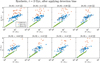Fig. 11

Mass-radius distribution of planets with different metallicity [Fe/H] from the synthetic population after applying the detection selection similar to PAST III.

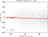Fig. 12

Host star metallicities vs. planet orbital period (grey dots) from the synthetic sample. The red line denotes the kernel regression of the mean metallicity of the planet population (from Equation (16)). The shaded red area shows the 68% (1-σ) confidence interval on the mean from bootstrapping. The dashed black line represents the mean metallicity (−0.05 ± 0.04 dex) for stars that host planets with a period >ten days. In the bottom-left corner, we print the Pearson coefficient R between host star metallicity and the orbital periods as well as the correspond p–value.

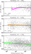Fig. 13

Similar to Fig. 12 for large planets (top), sub-Neptunes (middle), and terrestrial planets (bottom).

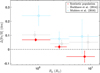Fig. 14

Difference in metallicity between stars hosting planets with orbital period P < 10 and >10 days. The solid red points and error bars show the results derived from the synthetic sample generated by the Bern model. The grey and cyan circles denote the results from Buchhave et al. (2014) and Mulders et al. (2016), respectively.

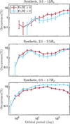Fig. 15

Planetary occurrence rate as a function of orbital period for super-solar and sub-solar metallicity stars derived from the synthetic population.

7 Orbital eccentricity versus metallicity

Orbital eccentricity is a fundamental planetary property, which contains important clues on the evolution history of planetary architectures. Plenty of statistical studies have found a positive correlation between stellar metallicity and planetary eccentricity both for giant planets (Dawson & Murray-Clay 2013; Buchhave et al. 2018) and smaller planets (Mills et al. 2019). In this section, using population synthesis, we investigate the correlation between stellar metallicity and planetary eccentricity and then compare with the observational results.

7.1 Giant planets

Dawson & Murray-Clay (2013) and Buchhave et al. (2018) collect data for giant planets from several radial velocity (RV) surveys (mainly HARPS, Lick, KICK; Fűrész et al. 2008; Telting et al. 2014; Butler et al. 2017; Trifonov et al. 2020). Since most of giant planets detected by RV only have measurements of minimum masses (M_p sin i), we also computed the minimum masses of planets (i.e. sin i) in the synthetic population using the following procedures: First, for each planetary system, we assumed the longitude ϕ and latitude θ of the line of sight of observer with respect to the reference frame of the given system obey a random distribution and obtain the unit vector of the direction of observer $\hat{o}$ $\[\hat{o}\]$ . Second, for a planets in a given system, we computed its orbital angular momentum with respect to the reference frame $\hat{h}$ $\[\hat{h}\]$ from its inclination i_p and longitude of the ascending node Ω_p. The formula of $\hat{o}$ $\[\hat{o}\]$ and $\hat{h}$ $\[\hat{h}\]$ are as follows: $\hat{o} = (\begin{matrix} \cos ϕ \sin θ \\ \sin ϕ \sin θ \\ \cos θ \end{matrix}) and \hat{h} = (\begin{matrix} \sin Ω_{p} \sin i_{p} \\ - \cos Ω_{p} \sin i_{p} \\ \cos i_{p} . \end{matrix}) .$ $\[\hat{o}=\left(\begin{array}{c}\cos~ \phi ~\sin~ \theta \\\sin~ \phi ~\sin~ \theta \\\cos~ \theta\end{array}\right) \text { and } \hat{h}=\left(\begin{array}{c}\sin~ \Omega_{\mathrm{p}} ~\sin~ i_{\mathrm{p}} \\-\cos~ \Omega_{\mathrm{p}} ~\sin~ i_{\mathrm{p}} \\\cos~ i_{\mathrm{p}}.\end{array}\right).\]$ (19)

Finally, the inclination of the orbit of the planet with respect to the observer i is the angle between $\hat{o}$ $\[\hat{o}\]$ and $\hat{h}$ $\[\hat{h}\]$ . Thus, $\cos i = \hat{o} * \hat{h}, \sin i = \sqrt{1 - \cos^{2} i} .$ $\[\cos~ i=\hat{o} * \hat{h}, ~\sin~ i=\sqrt{1-\cos~ ^2 i}.\]$ (20)

With similar criteria as these works, we selected planets with minimum masses in the range of 0.1–13 Jupiter mass (M_J) as giant planets from the synthetic population at 5 Gyr. To avoid the influence of tides (Bashi et al. 2024), we only considered planets with orbital semi-major axes a larger than 0.1 AU (e.g. Jackson et al. 2008; Lai 2012). Furthermore, to apply the similar detection bias as previous statistical studies (Dawson & MurrayClay 2013; Buchhave et al. 2018), we downloaded data from RV surveys (mainly HARPS, Lick, Keck; Fűrész et al. 2008; Telting et al. 2014; Butler et al. 2017; Trifonov et al. 2020) and obtained the median values of the root mean squares (RMS) of the semi-amplitudes and time baselines for Sun-like (i.e. FGK-type main-sequence) stars. Then we only kept giant planets with K > RMS_median & P < time baseline, where P is the orbital period and $K = \frac{28.4 m s^{- 1}}{\sqrt{1 - e^{2}}} \times \frac{M_{p} \sin i}{M_{J}} {(\frac{P}{1 y r})}^{- 1 / 3} {(\frac{M_{*}}{M_{⊙}})}^{- 2 / 3}$ $\[K=\frac{28.4 \mathrm{m} \mathrm{~s}^{-1}}{\sqrt{1-e^{2}}} \times \frac{M_{\mathrm{p}} ~\sin~ i}{M_{J}}\left(\frac{P}{1 \mathrm{yr}}\right)^{-1 / 3}\left(\frac{M_{*}}{M_{\odot}}\right)^{-2 / 3}\]$ is the amplitude of the generated RV signal. After applying the above selections, we were left with 155 stars hosting 240 planets. Figure 16 displays the M_p sin i − a diagram of giant planets in our sample.

Figure 17 shows the planetary eccentricity-stellar [Fe/H] diagram for giant planets in the biased RV sample (above the detection limit). We performed the Pearson test and the resulting to a Pearson coefficient of 0.10 with a p– value of 0.048, suggesting a positive eccentricity-metallicity correlation for giant planets with ~2 − σ confidence. Referring to previous studies (Dawson & Murray-Clay 2013; Buchhave et al. 2018), we further divided them into two categories according to their eccentricities:

high-eccentricity e > 0.25 (46);
low-eccentricity e ≤ 0.25 (194);

As shown in Fig. 18, the stars hosting high-eccentricity giant planets have a larger distribution in [Fe/H] comparing to those hosting low-eccentricity giant planets. To evaluate the significance, we performed the two-sample KS tests. The resulting p–values are 0.092, suggesting high-eccentricity giant planets are preferentially hosted by metal-richer stars compared to low-eccentricity giant planets with confidence level of ~1–2σ. The average metallicities for stars hosting high-eccentricity and loweccentricity giant planets are 0.17 ± 0.02 and 0.12 ± 0.02 dex (uncertainties derived from bootstrapping), respectively.

Previous studies have proposed a potential explanation for the eccentricity-metallicity trends: metal-richer stars are more likely to form more giant planets and perturbations of outer giant planets could have pump up planetary eccentricities (Buchhave et al. 2018). To examine this explanation, we compared the distributions in [Fe/H] for stars hosting 1, 2, and 3+ giant planets (regardless of whether giant planets could be detected or not). As shown in the top panel of Fig. 19, stars that host more giant planets have a relatively higher [Fe/H]. To evaluate the significance, we performed the two-sample KS tests and the resulted p–values are 0.185 and 0.129 for stars that host 2 and 3+ giant planets compared to those with 1 giant planets, corresponding to confidence levels of ~1 − σ. In the bottom panel of Fig. 19, we then compared the distribution of the eccentricities of synthetic giant planets in systems with 1, 2 and 3+ giant planets. As can be seen, single giant planets have a smaller eccentricity distribution compared to those in systems with 2 and 3+ giant planets with KS p–values of 0.1855 and 0.0732. The higher stellar [Fe/H] and larger planetary eccentricity (though statistically insignificant) of giant planets accompanied by other giant planets are generally in agreement with the expectation and thus support that the proposed mechanism could help to explain why eccentric giant planets favour metal-rich stars.

The above synthetic results suggest that giant planets with high eccentricity tend to be hosted by metal-richer stars, which is generally consistent with the statistical results (see Fig. 2 of Buchhave et al. 2018). Nevertheless, compared to the synthetic sample, the observed high-eccentricity (low-eccentricity) giant planets have significantly larger (smaller) metallicities, with an average of 0.23 ± 0.04 (−0.07 ± 0.05), leading to a more significant correlation between eccentricity and metallicity in the observations. Such a discrepancy is not unexpected. Due to computational cost constraints, we only simulated the interactions between planets for the first 100 Myr. Long-term perturbations between giant planets can further excite their eccentricities. This could lead to a stronger eccentricity-metallicity correlation since giant planets tend to be hosted by metal-richer stars. Moreover, as discussed in Sect. 5.5 of Emsenhuber et al. (2023), the final number of giant planets in a given system may not be same as the total number originally formed, due to collisions and ejections (see their Fig. 16).

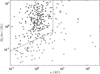Fig. 16

Semi-major axis (a) vs. effective mass (M_p sin i) for giant planets in the biased RV synthetic population at 5 Gyr. Solid points and open circles denote planets above and below the detection limit, respectively. The dashed line represents the typical detection limit for corresponding RV surveys when e = 0.

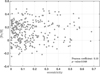Fig. 17

Planetary orbital eccentricity (e) vs. stellar metallicity ([Fe/H]) for giant planets in the synthetic population at 5 Gyr after selection according to the RV detection bias. We also print the Pearson coefficient and corresponding p–value.

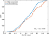Fig. 18

Cumulative distributions of stellar metallicities [Fe/H] for high-eccentricity (red) and low-eccentricity giant planets (blue). The two sample KS test p–value is printed in the corner.

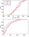Fig. 19

Cumulative distributions of stellar metallicities [Fe/H] (top panel) and planetary eccentricity (bottom panel) for single giant planetary systems (blue) and multiple giant planetary systems. The two sample KS test p–values are printed in the lower-right corner of each panel.

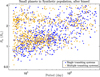Fig. 20

Orbital period (P) vs. radius (R_p) for selected small planets in the Kepler-biased synthetic population at 5 Gyr.

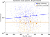Fig. 21

Orbital eccentricity vs. stellar metallicity ([Fe/H]) for Kepler-detectable small planets in single (blue) and multiple (orange) systems in the synthetic population. We also plot the mean planetary eccentricity and their 1-σ interval (50 ± 34.1% percentiles) from bootstrapping as solid diamonds and error bars. The best fits are plotted as solid lines.

7.2 Small planets

For the small planets with radii less than ~4 R_⊕, Mills et al. (2019) provides tentative evidence that eccentric small planets with radii between 1.4–4 R_⊕ favour metal-rich stars using the CKS sample. Recently, An et al. (2023) confirmed a significant eccentricity-metallicity trend for Kepler planets/candidates with R_p < 4 R_⊕ using LAMOST-Gaia-Kepler sample. In order to compare synthetic results with Kepler observational results, we first selected planets with R_p < 4 R_⊕ and orbital period P > 5 days with the same criteria as An et al. (2023) and then apply the detection biases using KOBE program (Mishra et al. 2021). Figure 20 shows the period-radius diagram for selected small planets in the Kepler-biased synthetic population.

Based on the selected synthetic sample, we investigate the orbital eccentricity e of small planets in single and multiple systems as a function of stellar [Fe/H]. Figure 21 displays the stellar [Fe/H]-planetary eccentricity diagram for small planets in single (blue) and multiple (orange) systems. As shown in Fig. 21, small planets in multiple systems are mostly on nearly circular orbits (with e ≲ 0.1), while small planets in single systems have a larger eccentricity distributions.

We adopted the two-sample KS test for the Kepler-biased synthetic sample and find that the eccentricity of small planets in single systems are significantly larger than those in multiple systems with a p–value of 7.9 × 10⁻¹³⁰, which is consistent with the ‘eccentricity-dichotomy’ revealed by Kepler data (Van Eylen & Albrecht 2015; Xie et al. 2016; Mills et al. 2019). Quantitatively, the average eccentricities of single systems ( $\bar{e}$ $\[\bar{e}\]$ ~ 0.140) and multiple systems ( $\bar{e}$ $\[\bar{e}\]$ ~ 0.05) from the synthetic sample are both well consistent with the observational results from California-Kepler Survey data, i.e. Rayleigh distributions with σ_e of ${0.167}_{- 0.0008}^{+ 0.0013}$ $\[0.167_{-0.0008}^{+0.0013}\]$ and 0.035 ± 0.006 Mills et al. (2019). Xie et al. (2016) derive a slightly large average eccentricity (~0.3) for planets in single systems and Mills et al. (2019) suggest that this discrepancy could be that the stellar properties using in Xie et al. (2016) have not be improved by the Gaia catalogues and result in a slightly higher eccentricity distribution.

Moreover, with the increase of stellar [Fe/H], the eccentricities of small planets in single system grow, while the eccentricity of small planets in multiple systems changes mildly. To quantify the correlation between e and [Fe/H], following An et al. (2023), we then divided the small planets in the synthetic sample into four bins according to their [Fe/H] and calculate their average orbital eccentricities $\bar{e}$ $\[\bar{e}\]$ , which is shown in Fig. 21. Then we fitted $\bar{e}$ $\[\bar{e}\]$ and [Fe/H] with a constant model ( $\bar{e}$ $\[\bar{e}\]$ = constant) and an exponential model ( $\bar{e} = a \times 10^{(b \times [F e / H]}$ $\[\bar{e}=a \times 10^{(b \times[\mathrm{Fe} / \mathrm{H}]}\]$ )) with the Levenberg-Marquardt algorithm (LMA). For the small planets in single systems, the exponential model is preferential compare to constant model with an AIC difference (ΔAIC) of 6.5. In contrast, for planets in multiple systems, the constant model is preferred with a smaller AIC score (ΔAIC = −0.8). In order to obtain the uncertainties of $\bar{e}$ $\[\bar{e}\]$ and evaluate the significance, we generated the 1000 bootstrapped sample from the original sample and calculate the mean eccentricities for the four bins. The uncertainty was set as the 50 ± 34.1 percentiles in the resampled distribution. Then we refitted the $\bar{e}$ $\[\bar{e}\]$ –[Fe/H] relation with the same procedure before. Out of the 1000 sets of resampled data, the exponential model is preferred with a smaller AIC score for 961 times for the small planets in single systems (corresponding to a confidence level of 96.1%), while for those in multiple systems, the constant model is preferred for 816 times. The fitting results of the preferred models are: $\bar{e} = {\begin{array}{lc} {0.12}_{- 0.01}^{+ 0.01} \times 10^{({0.26}_{- 0.07}^{+ 0.08} \times [F e / H])} & Single \\ {0.05}_{- 0.01}^{+ 0.01} & Multiple . \end{array}$ $\[\bar{e}=\left\{\begin{array}{lc}0.12_{-0.01}^{+0.01} \times 10^{\left(0.26_{-0.07}^{+0.08} \times[\mathrm{Fe} / \mathrm{H}]\right)} & \text { Single } \\0.05_{-0.01}^{+0.01} & \text { Multiple }.\end{array}\right.\]$ (21)

Referring to Mills et al. (2019), we further divided small planets into two subsamples, i.e. radii larger or smaller than 1.4 R_⊕. We find that e of planets in single systems exists positive correlations with [Fe/H] with Pearson coefficients of 0.11 (corresponding p–value of 1.1 × 10⁻⁸) and 0.03 (corresponding P–value of 0.010) for the two subsamples of R_p ≥ and < 1.4 R_⊕, respectively. The exponential model is preferential compare to constant model with AIC difference of 4.6 and 6.3 for the two subsamples of R_p ≥ 1.4 R_⊕ and 1.4 R_⊕ respectively, corresponding to confidence levels of ≳2σ). The fitting results of the exponential models are: $\bar{e} = {\begin{cases} 0.11 \times 10^{(0.4 \times [F e / H])} & R_{p} \geq 1.4 R_{\oplus}, Single \\ 0.22 \times 10^{(0.2 \times [F e / H])} & R_{p} < 1.4 R_{\oplus}, Single . \end{cases}$ $\[\bar{e}= \begin{cases}0.11 \times 10^{(0.4 \times[\mathrm{Fe} / \mathrm{H}])} & R_{\mathrm{p}} \geq 1.4 ~R_{\oplus}, \text { Single } \\ 0.22 \times 10^{(0.2 \times[\mathrm{Fe} / \mathrm{H}])} & R_{\mathrm{p}}<1.4 ~R_{\oplus}, \text { Single }.\end{cases}\]$ (22)

In contrast, for planets in multiple systems, the correlations with [Fe/H] are statistically indistinguishable with Pearson coefficients of only 0.01 (corresponding p–value of 0.63) and −0.06 (corresponding p–value of 0.07) for the two subsamples, respectively. Moreover, the constant model is preferred with smaller AIC score for both the two subsamples.

Based on the above trends, we conclude that on average, small planets in single systems are on eccentric orbits and their eccentricities increase with [Fe/H], while small planets in multiple systems are mostly on near-circular orbits and their eccentricities shows no (significant) dependence on [Fe/H]. That is to say, the ‘eccentricity dichotomy’ becomes more significant with increasing [Fe/H].

One potential explanation for the positive eccentricity-metallicity relation of small planets in the single transiting systems is that protoplanetary discs with higher metallicities have more solid materials to form more giant planets, and the gravitational perturbations by outer giant planets would pump up larger orbital eccentricities of inner small planets (Huang et al. 2017; Pu & Lai 2018; Poon & Nelson 2020). To examine the above explanation, we classified these single transiting small planets into two categories: with and without outer giant planets (OGP). In the top panel of Fig. 22, we show the fraction of single transiting planets with OGPs F_OGP as a function of stellar metallicity. As can be seen, F_OGP grows from 1% to 30% when [Fe/H] increases from −0.2 to 0.2, which is expected since giant planets are more preferred to be hosted by metal-richer stars compared to small planets (see Figs. 2 and 4). Then we divided these two categories into four bins according to [Fe/H] with the same interval shown in Fig. 21 and calculate the mean eccentricities and corresponding uncertainties. As can be seen in the bottom panel of Fig. 22, there exists an obviously positive correlation between e − [Fe/H] for single transiting planets with OGPs. In contrast, the eccentricities of single transiting planets without OGPs are more dispersed and show no significant dependence on metallicity.

To qualify the $\bar{e}$ $\[\bar{e}\]$ –[Fe/H] correlation for single transiting planets with/without OGPs, we fitted them by adopting the same procedure as before. For single transiting planets with OGPs, the exponential model is preferred with ΔAIC of 13.1, corresponding to a confidence level of 99.9% from the bootstrapping. In contrast, the constant model is preferred with a smaller AIC score (ΔAIC = −0.96) for the single transiting planets without OGPs. The best fits are: $\bar{e} = {\begin{array}{lc} {0.10}_{- 0.01}^{+ 0.01} \times 10^{({1.61}_{- 0.15}^{+ 0.21} \times [F e / H])} & Single with OGPs \\ {0.12}_{- 0.01}^{+ 0.01} & Single without OGPs . \end{array}$ $\[\bar{e}=\left\{\begin{array}{lc}0.10_{-0.01}^{+0.01} \times 10^{\left(1.61_{-0.15}^{+0.21} \times[\mathrm{Fe} / \mathrm{H}]\right)} & \text { Single with OGPs} \\0.12_{-0.01}^{+0.01} & \text { Single without OGPs}.\end{array}\right.\]$ (23)

Out of the 1000 sets of resampled data, the exponential indexes of single small planets with OGPs are all larger than those of small planets without OGPs, suggesting that the perturbations by outer giant planets help to excite the orbital eccentricities of inner small planets. Moreover, the best fit of the $\bar{e}$ $\[\bar{e}\]$ –[Fe/H] relation for the single planets with OGPs in the synthetic population is well consistent with the result derived from the LAMOST-Gaia-Kepler sample $(\bar{e} = {0.11}_{- 0.06}^{+ 0.06} \times 10^{({1.78}_{- 0.89}^{+ 1.49} \times [F e / H])}$ $\[\bar{e}=0.11_{-0.06}^{+0.06} \times 10^{\left(1.78_{-0.89}^{+1.49} \times[\mathrm{Fe} / \mathrm{H}]\right)}\]$ ; An et al. 2023). The above analyses demonstrate that the external eccentricity exciting mechanism could explain the positive eccentricity-metallicity correlation for inner small planets accompanied by OGPs.

Nevertheless, for those with no OGPs, their eccentricities are independent with stellar [Fe/H], which is inconsistent with the observational results. This is not unexpected since our model only consider the interaction between planets for the first 100 Myr and thus does not include the long-term formation and evolution of small planets, which are discussed as follows:

For single transiting small planets without OGPs in the synthetic sample, nearly all (96.9%) are accompanied by at least one undetectable small planet (1–4 R_⊕, 5 < P < 400 d) according to Kepler’s detection limits. In contrast, the majority (73%) of single transiting small planets with OGPs lack any small planet companions. Theoretical studies and simulations have demonstrated that long-term dynamical interactions among inner small planets can pump up the orbital eccentricity/inclination of planets (e.g. Zhou et al. 2007; Moriarty & Ballard 2016), which is also supported by observations, as the Kepler sample reveals that planetary systems become dynamically hotter (with higher eccentricity/inclination dispersion) as stars age (e.g. Chen et al. 2021; Yang et al. 2023). The average eccentricity of small planets, induced by long-term perturbations of nearby planets, is estimated to be (Zhou et al. 2007): $< e^{2} >^{1 / 2} \approx 5.2 k_{0}^{- 3 / 2} μ^{1 / 2} {(\frac{t}{y r})}^{1 / 2},$ $\[<e^2>^{1 / 2} ~\approx ~5.2 k_0^{-3 / 2} \mu^{1 / 2}\left(\frac{t}{\mathrm{yr}}\right)^{1 / 2},\]$ (24)

where k₀ is the scaled initial separation. μ is the average mass of small planets in one system. Figure 23 displays the average masses of small planets (regardless whether could be detected or not) in single transiting systems without OGPs as a function of metallicity. As can be seen, the average masses μ show an obviously positive correlation with [Fe/H] (Pearson coefficient of 0.39 with a p– value of 1.0 × 10⁻¹³⁰) and μ ~ 5 M_⊕ × 10^{(0.7×[Fe/H])}, which would lead to an increase in the exponential index by ~0.35.
Some small planets may even experience merge/ejection due to the interaction of close planets (e.g. Pu & Wu 2015), especially for planets with lower masses, since they are expected to have larger amplitudes of the eccentricity (e.g. Lithwick & Wu 2011). This would remove some eccentric planets (e > 0.3) with lower masses (mostly with R_p < 1.7 R_⊕) around stars with sub-solar metallicities ([Fe/H] ≲ −0.1 dex) in the synthetic sample, which would further increase the exponential index and help to explain why such planets are absent in the observed sample (see Figs. 6, 8 and 10 of An et al. (2023), e > 0.3 are beyond 3-σ for stars of [Fe/H] ≲ −0.1).

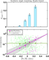Fig. 22

Top: fraction of single transiting small planets with outer giant planets (OGP) vs. stellar metallicities derived from the Kepler-biased synthetic sample. Bottom: Orbital eccentricity vs. stellar metallicity for small transiting planets with and without OGPs (purple/green). The solid lines represent the corresponding best fits. The grey region denotes the 1 − σ interval of the eccentricity-[Fe/H] correlation derived from the LAMOST-Gaia-Kepler sample (An et al. 2023).

Table 1

Dependence of the planetary properties as a function of stellar [Fe/H] derived from the synthetic NG76Longshot population.

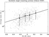Fig. 23

Average masses of small planets (regardless of whether they could be detected or not) in single transiting systems without OGPs vs. stellar metallicity (grey circles). The diamonds and error bars denote the mean and 1-σ (50 ± 34.1) interval of the average masses in different bins of [Fe/H]. The solid line represents the best fit.

8 Summary

In this work, based on the synthetic planet population (Sect. 3) generated by the Bern Generation III model (Sect. 2), we performed a series of statistical analyses of planet properties as a function of stellar metallicity and compare with observational results. These results are summarized in Table 1.

We first investigate the dependence of the occurrence rates, F, of planets with different sizes on the stellar metallicity (see Sect. 4). The main results are summarized as follows: (1) The occurrence rates of the synthetic hot, warm, and cold giant planets and Neptune-sized planets show significantly positive correlations (Sects. 4.1–4.2, Figs. 2–3). We performed a Bayesian analysis using an exponential model F ∝ 10^{β×10^[Fe/H]}. The resulted β are ~1.3 and ~0.5–0.8 for the giant planets and Neptune-sized planets, respectively. (2) For the Kepler planets with radii between 1–3.5 R_⊕, their occurrence rate, F, as well as the fraction of stars that host planets, η_system, and average multiplicity, k, generally increase and then decrease with increasing [Fe/H] and the inflection point is ~0.1 dex (Sect. 4.3, Fig. 4). After excluding planetary systems with large planets (R_p > 3.5 R_⊕), the decreases in F (as well as k and η_system) at [Fe/H] > 0.1 become weaker (see Fig. 5), which suggests that the perturbation by large planets around metal-richer stars is an important mechanism that causes the above inflection in the occurrence of Kepler-like planets. (3) For sub-Earths with R_p < 1 R_⊕, their occurrence rate, F, as well as two decomposed factors η_system and k all decline significantly with increasing [Fe/H] (Sect. 4.4, Fig. 6). The occurrence rate-metallicity correlations derived from synthetic populations are generally consistent with the observational results for giant planets (e.g. Fischer & Valenti 2005; Johnson et al. 2010; Chen et al. 2023), Neptune-sized planets (e.g. Dong et al. 2018; Petigura et al. 2018; Chen et al. 2022), and Kepler planets (e.g. Wang & Fischer 2015; Petigura et al. 2018; Zhu 2019).

We then study the radius valley morphology as a function of [Fe/H] using the synthetic population after applying the Kepler detection biases (Sect. 5). We find that the radius valley deepens and the number ratio of super-Earths to sub-Neptunes decreases with increasing [Fe/H]. The fraction of Neptune-sized planets and the average radii of planets above the radius valley are found to increase with [Fe/H], while the average radii of planets below the radius valley (1–1.7 R_⊕) are broadly unchanged (Figs. 8–9). The evolutional trends of the five metrics are quantitatively consistent with those of Chen et al. (2022) derived from the LAMOST-Gaia-Kepler sample. The good matches between our nominal model and observations support that the observed radius valley can be interpreted as the separation of two distinct planet populations, i.e. less massive, rocky super-Earths formed in situ and more massive water-rich sub-Neptunes formed ex-situ beyond the ice-line that then migrated inwards (Venturini et al. 2020; Burn et al. 2024a).

In Sect. 6, we explore how the period distributions of the synthetic planet populations depend on [Fe/H]. We find that the orbital periods of synthetic planets are anti-correlated with [Fe/H] and planets with orbital periods less than ten days are preferentially to be hosted by metal-richer stars with a difference in stellar metallicity Δ[Fe/H] of 0.05 ± 0.01 dex compared to those with longer periods (Fig. 12). The results also show that the anti-correlation (as well as Δ[Fe/H]) is most significant (largest as 0.07 ± 0.01 dex) for the terrestrial planets and becomes weaker with the increase of planet size (Figs. 13–14). The above synthetic results are qualitatively consistent with the observational results (Buchhave et al. 2014; Mulders et al. 2016).

Finally, we investigate the correlations between the orbital eccentricity and host star [Fe/H]. We find that giant planets in eccentric orbits (e > 0.25) are preferentially to be hosted by metal-rich stars (Fig. 18). For small planets in single transiting systems, their eccentricities increase with stellar metallicities, while the eccentricities of small planets in multiple transiting systems are on average lower and have no significant correlation with [Fe/H] (Fig. 21). Our results also show that metal-richer stars are more likely to be accompanied by (multiple) giant planets (top panels of Figs. 19 and 22) and thus the perturbations by giant planets are stronger to pump up the eccentricities of giant planets and small planets (bottom panels of Figs. 19 and 22). Furthermore, the average masses of small planets increase significantly with [Fe/H] (Fig. 23) and thus the self-interaction should be stronger, which further strengthens the eccentricity-metallicity correlation for small planets.

Overall, the synthetic population can generally reproduce the observed correlations between stellar metallicities and occurrence rates (e.g. Fischer & Valenti 2005; Johnson et al. 2010; Wang & Fischer 2015; Weiss et al. 2018; Petigura et al. 2018; Zhu 2019; Chen et al. 2023), radius valley morphology (Pu & Lai 2018; Chen et al. 2022), orbital periods (Buchhave et al. 2014; Mulders et al. 2016), and eccentricity (Dawson & MurrayClay 2013; Buchhave et al. 2018; An et al. 2023). Nevertheless, the dependence of orbital period and eccentricity on the stellar metallicity derived from the synthetic sample are significantly weaker than that from observations. Potential reasons could be: (1) the Generation III Bern model only considers the interactions between planets for the first 100 Myr and thus does not include the effect of the long-term evolution of planets (Emsenhuber et al. 2021a). (2) The effects of the stellar cluster environment at birth and binary companions are not included in the current model.

Future observations from both space and ground-based instruments (e.g. GAIA, PLATO, NIRPS, ROMAN, ARIEL) will provide additional observational datasets and relevant statistical analyses will provide more observational clues and constraints for planet formation and evolution. Via planetary population synthesis, theoretical planet formation models can use this as an opportunity to perform not only qualitative but also quantitative comparisons in global ways between the synthetic population and observational datasets. The approach is particularly constraining if the same synthetic population is compared to datasets obtained from different observational methods, as is done here where the NGPPS VII paper (Emsenhuber et al. 2025) compares the same population as that used here with the constraints from the HARPS/Coralie GTO survey (Mayor et al. 2011). The reason is that different methods probe different model aspects. Such a quantitative multi-method approach will reveal the success and limitations of our current understanding of planet formation more clearly and will eventually help to refine the theory of planet formation and evolution.

Acknowledgements

This work is supported by the National Key R&D Program of China (2024YFA1611803) and the National Natural Science Foundation of China (NSFC; grant no. 12273011, 12150009, 12403071). This research is also supported by the Excellence Cluster ORIGINS which is funded by the Deutsche Forschungsgemeinschaft (DFG, German Research Foundation) under Germany’s Excelence Strategy – EXC-2094-390783311. C.M. and A.E. acknowledge the support from the Swiss National Science Foundation under grant 200021_204847 “PlanetsInTime”. R.B. acknowledges the financial support from DFG under Germany’s Excellence Strategy EXC 2181/1-390900948, Exploratory project EP 8.4 (the Heidelberg STRUCTURES Excellence Cluster). Parts of this work has been carried out within the framework of the NCCR PlanetS supported by the Swiss National Science Foundation under grants 51NF40_182901 and 51NF40_205606. J.-W.X. also acknowledges the support from the National Youth Talent Support Program.

References

Alibert, Y., Mordasini, C., Benz, W., et al. 2005, A&A, 434, 343 [NASA ADS] [CrossRef] [EDP Sciences] [Google Scholar]
An, D.-S., Xie, J.-W., Dai, Y.-Z., et al. 2023, AJ, 165, 125 [Google Scholar]
Andrews, S. M., Wilner, D. J., Hughes, A. M., et al. 2010, ApJ, 723, 1241 [NASA ADS] [CrossRef] [Google Scholar]
Ayliffe, B. A., & Bate, M. R. 2012, MNRAS, 427, 2597 [Google Scholar]
Baruteau, C., Crida, A., Paardekooper, S.-J., et al. 2014, Protostars and Planets VI, 667 [Google Scholar]
Baruteau, C., & Zhu, Z. 2016, MNRAS, 458, 3927 [NASA ADS] [CrossRef] [Google Scholar]
Bashi D., Mazeh T., & Faigler S., 2024, AJ, 168, 115 [Google Scholar]
Berger, T. A., Huber, D., Gaidos, E., et al. 2020, AJ, 160, 108 [NASA ADS] [CrossRef] [Google Scholar]
Benítez-Llambay, P., Masset, F., & Beaugé, C. 2011, A&A, 528, A2 [NASA ADS] [CrossRef] [EDP Sciences] [Google Scholar]
Bodenheimer, P., & Pollack, J. B. 1986, Icarus, 67, 391 [Google Scholar]
Bodenheimer, P., Hubickyj, O., & Lissauer, J. J. 2000, Icarus, 143, 2 [Google Scholar]
Borucki, W. J., Koch, D., Basri, G., et al. 2010, Science, 327, 977 [Google Scholar]
Buchhave, L. A., Latham, D. W., Johansen, A., et al. 2012, Nature, 486, 375 [NASA ADS] [Google Scholar]
Buchhave, L. A., Bizzarro, M., Latham, D. W., et al. 2014, Nature, 509, 593 [Google Scholar]
Buchhave, L. A., Bitsch, B., Johansen, A., et al. 2018, ApJ, 856, 37 [Google Scholar]
Burn, R., & Mordasini, C. 2024, Handbook of Exoplanets, 2nd edn., eds. H. Deeg & J. Antonio Belmonte (Springer International Publishing), 143-2 [Google Scholar]
Burn, R., Schlecker, M., Mordasini, C., et al. 2021, A&A, 656, A72 [NASA ADS] [CrossRef] [EDP Sciences] [Google Scholar]
Burn, R., Mordasini, C., Mishra, L., et al. 2024a, Nat. Astron., 8, 463 [Google Scholar]
Burn, R., Bali, K., Dorn, C., et al. 2024b, A&A, submitted [arXiv:2411.16879] [Google Scholar]
Butler, R. P., Vogt, S. S., Laughlin, G., et al. 2017, AJ, 153, 208 [Google Scholar]
Chabrier, G., Mazevet, S., & Soubiran, F. 2019, ApJ, 872, 51 [NASA ADS] [CrossRef] [Google Scholar]
Chambers, J. E. 1999, MNRAS, 304, 793 [Google Scholar]
Chambers, J. E. 2001, Icarus, 152, 205 [Google Scholar]
Chambers, J. 2006, Icarus, 180, 496 [NASA ADS] [CrossRef] [Google Scholar]
Chen, D.-C., Yang, J.-Y., Xie, J.-W., et al. 2021, AJ, 162, 100 [NASA ADS] [CrossRef] [Google Scholar]
Chen, D.-C., Xie, J.-W., Zhou, J.-L., et al. 2022, AJ, 163, 249 [NASA ADS] [CrossRef] [Google Scholar]
Chen, D.-C., Xie, J.-W., Zhou, J.-L., et al. 2023, PNAS, 120, e2304179120 [NASA ADS] [CrossRef] [Google Scholar]
Chen, D.-C., Mordasini, C., Xie, J.-W., et al. 2024, A&A, 687, A25 [NASA ADS] [CrossRef] [EDP Sciences] [Google Scholar]
Chen, D.-C., Xie, J.-W., et al. 2025, Nat. Astron., submitted [Google Scholar]
Christian, D. J., Pollacco, D. L., Skillen, I., et al. 2006, MNRAS, 372, 1117 [NASA ADS] [CrossRef] [Google Scholar]
Clarke, C. J., Gendrin, A., & Sotomayor, M. 2001, MNRAS, 328, 485 [NASA ADS] [CrossRef] [Google Scholar]
Coleman, G. A. L., & Nelson, R. P. 2014, MNRAS, 445, 479 [Google Scholar]
Crida, A., Morbidelli, A., & Masset, F. 2006, Icarus, 181, 587 [Google Scholar]
Dawson, R. I., & Johnson, J. A., 2018, ARA&A, 56, 175 [Google Scholar]
Dawson, R. I. & Murray-Clay, R. A., 2013, ApJ, 767, L24 [Google Scholar]
Dittkrist, K.-M., Mordasini, C., Klahr, H., et al. 2014, A&A, 567, A121 [NASA ADS] [CrossRef] [EDP Sciences] [Google Scholar]
Dong, S., Xie, J.-W., Zhou, J.-L., et al. 2018, PNAS, 115, 266 [NASA ADS] [CrossRef] [Google Scholar]
Doyle, L., Armstrong, D. J., Acuña, L., et al. 2025, MNRAS, 539, 3138 [Google Scholar]
Emsenhuber, A., Mordasini, C., Burn, R., et al. 2021a, A&A, 656, A69 [NASA ADS] [CrossRef] [EDP Sciences] [Google Scholar]
Emsenhuber, A., Mordasini, C., Burn, R., et al. 2021b, A&A, 656, A70 [NASA ADS] [CrossRef] [EDP Sciences] [Google Scholar]
Emsenhuber, A., Mordasini, C., & Burn, R. 2023, Eur. Phys. J. Plus, 138, 181 [NASA ADS] [CrossRef] [Google Scholar]
Emsenhuber, A., Mordasini, C., Mayor, M., et al. 2025, A&A, 701, A64 [NASA ADS] [CrossRef] [EDP Sciences] [Google Scholar]
Fabrycky, D., & Tremaine, S. 2007, ApJ, 669, 1298 [NASA ADS] [CrossRef] [Google Scholar]
Fabrycky, D. C., Lissauer, J. J., Ragozzine, D., et al. 2014, ApJ, 790, 146 [Google Scholar]
Ferraz-Mello, S., Rodríguez, A., & Hussmann, H. 2008, Celest. Mech. Dyn. Astron., 101, 171 [Google Scholar]
Fischer, D. A., & Valenti, J. 2005, ApJ, 622, 1102 [NASA ADS] [CrossRef] [Google Scholar]
Fischer, D. A., Marcy, G. W., & Spronck, J. F. P. 2014, ApJS, 210, 5 [Google Scholar]
Fortier, A., Alibert, Y., Carron, F., et al. 2013, A&A, 549, A44 [NASA ADS] [CrossRef] [EDP Sciences] [Google Scholar]
Freedman, R. S., Lustig-Yaeger, J., Fortney, J. J., et al. 2014, ApJS, 214, 25 [CrossRef] [Google Scholar]
Fulton, B. J., Petigura, E. A., Howard, A. W., et al. 2017, AJ, 154, 109 [Google Scholar]
Fűrész, G., Szentgyorgyi, A. H., & Meibom, S. 2008, Precis. Spectrosc. Astrophys., 287 [Google Scholar]
Guo, X., Johnson, J. A., Mann, A. W., et al. 2017, ApJ, 838, 25 [NASA ADS] [CrossRef] [Google Scholar]
Haldemann, J., Alibert, Y., Mordasini, C., et al. 2020, A&A, 643, A105 [NASA ADS] [CrossRef] [EDP Sciences] [Google Scholar]
Hamer, J. H., & Schlaufman, K. C. 2022, AJ, 164, 26 [NASA ADS] [CrossRef] [Google Scholar]
Ho, C. S. K., & Van Eylen, V. 2023, MNRAS, 519, 4056 [NASA ADS] [CrossRef] [Google Scholar]
Ho, C. S. K., Rogers, J. G., Van Eylen, V., Owen, J. E., & Schlichting, H. E. 2024, MNRAS, 531, 3698 [NASA ADS] [CrossRef] [Google Scholar]
Holl, B., Sozzetti, A., Sahlmann, J., et al. 2022, VizieR Online Data Catalog: 367. J/A+A/674/A10 [Google Scholar]
Hsu, D. C., Ford, E. B., Ragozzine, D., et al. 2019, AJ, 158, 109 [NASA ADS] [CrossRef] [Google Scholar]
Huang, C. X., Petrovich, C., & Deibert, E. 2017, AJ, 153, 210 [NASA ADS] [CrossRef] [Google Scholar]
Ida, S., & Lin, D. N. C. 2004, ApJ, 616, 567 [NASA ADS] [CrossRef] [Google Scholar]
Ida, S., & Makino, J. 1993, Icarus, 106, 210 [NASA ADS] [CrossRef] [Google Scholar]
Jackson, B., Greenberg, R., & Barnes, R. 2008, ApJ, 678, 1396 [Google Scholar]
Jackson, B., Barnes, R., & Greenberg, R. 2009, ApJ, 698, 1357 [Google Scholar]
Jin, S., & Mordasini, C. 2018, ApJ, 853, 163 [Google Scholar]
Jin, S., Mordasini, C., Parmentier, V., et al. 2014, ApJ, 795, 65 [Google Scholar]
Johnson, J. A., Aller, K. M., Howard, A. W., et al. 2010, PASP, 122, 905 [Google Scholar]
Johnstone, C. P. 2020, ApJ, 890, 79 [Google Scholar]
Kama, M., Min, M., & Dominik, C. 2009, A&A, 506, 1199 [NASA ADS] [CrossRef] [EDP Sciences] [Google Scholar]
Kite, E. S., Fegley, B., Schaefer, L., et al. 2019, ApJ, 887, L33 [NASA ADS] [CrossRef] [Google Scholar]
Kubyshkina, D. I., & Fossati, L. 2021, RNAAS, 5, 74 [NASA ADS] [Google Scholar]
Kubyshkina, D., Fossati, L., Erkaev, N. V., et al. 2018, A&A, 619, A151 [NASA ADS] [CrossRef] [EDP Sciences] [Google Scholar]
Lai, D., & Pu, B. 2017, AJ, 153, 42 [Google Scholar]
Lai, D. 2012, MNRAS, 423, 486 [NASA ADS] [CrossRef] [Google Scholar]
Lithwick, Y., & Wu, Y. 2011, ApJ, 739, 31 [NASA ADS] [CrossRef] [Google Scholar]
Liu, B., Lambrechts, M., Johansen, A., et al. 2019, A&A, 632, A7 [NASA ADS] [CrossRef] [EDP Sciences] [Google Scholar]
Lodders, K. 2003, ApJ, 591, 1220 [Google Scholar]
Lopez, E. D., & Fortney, J. J. 2013, ApJ, 776, 2 [Google Scholar]
Luque, R., & Pallé, E. 2022, Science, 377, 1211 [NASA ADS] [CrossRef] [Google Scholar]
Lüst, R. 1952, Zeitsch. Naturfor. A, 7, 87 [CrossRef] [Google Scholar]
Lynden-Bell, D., & Pringle, J. E. 1974, MNRAS, 168, 603 [Google Scholar]
Marboeuf, U., Thiabaud, A., Alibert, Y., et al. 2014, A&A, 570, A35 [NASA ADS] [CrossRef] [EDP Sciences] [Google Scholar]
Martinez, C. F., Cunha, K., Ghezzi, L., et al. 2019, ApJ, 875, 29 [CrossRef] [Google Scholar]
Matsuyama, I., Johnstone, D., & Hartmann, L. 2003, ApJ, 582, 893 [NASA ADS] [CrossRef] [Google Scholar]
Mayor, M., Marmier, M., Lovis, C., et al. 2011, arXiv e-prints [arXiv:1109.2497] [Google Scholar]
Mills, S. M., Howard, A. W., Petigura, E. A., et al. 2019, AJ, 157, 198 [Google Scholar]
Mishra, L., Alibert, Y., Leleu, A., et al. 2021, A&A, 656, A74 [NASA ADS] [CrossRef] [EDP Sciences] [Google Scholar]
Mizuno, H. 1980, Progr. Theor. Phys., 64, 544 [CrossRef] [Google Scholar]
Mordasini, C. 2020, A&A, 638, A52 [NASA ADS] [CrossRef] [EDP Sciences] [Google Scholar]
Mordasini, C., Alibert, Y., & Benz, W. 2009a, A&A, 501, 1139 [NASA ADS] [CrossRef] [EDP Sciences] [Google Scholar]
Mordasini, C., Alibert, Y., Benz, W., et al. 2009b, A&A, 501, 1161 [NASA ADS] [CrossRef] [EDP Sciences] [Google Scholar]
Mordasini, C., Alibert, Y., Klahr, H., et al. 2012, A&A, 547, A111 [NASA ADS] [CrossRef] [EDP Sciences] [Google Scholar]
Mordasini, C., Mollière, P., Dittkrist, K.-M., et al. 2015, Int. J. Astrobiol., 14, 201 [NASA ADS] [CrossRef] [Google Scholar]
Moriarty, J., & Ballard, S. 2016, ApJ, 832, 34 [Google Scholar]
Mulders, G. D., Pascucci, I., Apai, D., et al. 2016, AJ, 152, 187 [NASA ADS] [CrossRef] [Google Scholar]
Mulders, G. D. 2018, Handbook of Exoplanets, 153 [Google Scholar]
Mulders, G. D., Mordasini, C., Pascucci, I., et al. 2019, ApJ, 887, 157 [NASA ADS] [CrossRef] [Google Scholar]
Nakamoto, T., & Nakagawa, Y. 1994, ApJ, 421, 640 [Google Scholar]
Neil, A. R., & Rogers, L. A. 2020, ApJ, 891, 12 [Google Scholar]
Ormel, C. W., & Klahr, H. H. 2010, A&A, 520, A43 [NASA ADS] [CrossRef] [EDP Sciences] [Google Scholar]
Owen, J. E., & Wu, Y. 2017, ApJ, 847, 29 [Google Scholar]
Owen, J. E., & Wu, Y. 2013, ApJ, 775, 105 [Google Scholar]
Owen, J. E., & Murray-Clay, R. 2018, MNRAS, 480, 2206 [NASA ADS] [CrossRef] [Google Scholar]
Pan, M., Liu, B., Jiang, L., et al. 2025, ApJ, 985, 1, 7 [Google Scholar]
Perri, F., & Cameron, A. G. W. 1974, Icarus, 22, 416 [Google Scholar]
Petigura, E. A., Marcy, G. W., Winn, J. N., et al. 2018, AJ, 155, 89 [Google Scholar]
Pollack, J. B., Hubickyj, O., Bodenheimer, P., et al. 1996, Icarus, 124, 62 [NASA ADS] [CrossRef] [Google Scholar]
Poon, S. T. S., & Nelson, R. P. 2020, MNRAS, 498, 5166 [NASA ADS] [CrossRef] [Google Scholar]
Pu, B., & Lai, D. 2018, MNRAS, 478, 197 [NASA ADS] [CrossRef] [Google Scholar]
Pu, B., & Wu, Y. 2015, ApJ, 807, 44 [Google Scholar]
Qian, Y., & Wu, Y. 2021, AJ, 161, 201 [NASA ADS] [CrossRef] [Google Scholar]
Raymond, S. N., & Morbidelli, A. 2022, Demographics of Exoplanetary Systems, Lecture Notes of the 3rd Advanced School on Exoplanetary Science, 466, 3 [Google Scholar]
Rafikov, R. R. 2004, AJ, 128, 1348 [NASA ADS] [CrossRef] [Google Scholar]
Ricker, G. R., Winn, J. N., Vanderspek, R., et al. 2015, J. Astron. Telesc. Instrum. Syst., 1, 014003 [Google Scholar]
Santos, N. C., Israelian, G., & Mayor, M. 2001, A&A, 373, 1019 [NASA ADS] [CrossRef] [EDP Sciences] [Google Scholar]
Santos, N. C., Israelian, G., & Mayor, M. 2004, A&A, 415, 1153 [NASA ADS] [CrossRef] [EDP Sciences] [Google Scholar]
Schlecker, M., Mordasini, C., Emsenhuber, A., et al. 2021, A&A, 656, A71 [NASA ADS] [CrossRef] [EDP Sciences] [Google Scholar]
Shakura, N. I., & Sunyaev, R. A. 1973, A&A, 24, 337 [NASA ADS] [Google Scholar]
Shibata, S., Helled, R., & Ikoma, M. 2020, A&A, 633, A33 [NASA ADS] [CrossRef] [EDP Sciences] [Google Scholar]
Telting, J. H., Avila, G., Buchhave, L., et al. 2014, Astron. Nachr., 335, 41 [Google Scholar]
Thiabaud, A., Marboeuf, U., Alibert, Y., et al. 2014, A&A, 562, A27 [NASA ADS] [CrossRef] [EDP Sciences] [Google Scholar]
Thompson, S. E., Coughlin, J. L., Hoffman, K., et al. 2018, ApJS, 235, 38 [NASA ADS] [CrossRef] [Google Scholar]
Thommes, E. W., Duncan, M. J., & Levison, H. F. 2003, Icarus, 161, 431 [NASA ADS] [CrossRef] [Google Scholar]
Trifonov, T., Tal-Or, L., Zechmeister, M., et al. 2020, A&A, 636, A74 [NASA ADS] [CrossRef] [EDP Sciences] [Google Scholar]
Tychoniec, Ł., Tobin, J. J., Karska, A., et al. 2018, ApJS, 238, 19 [Google Scholar]
Udry, S., & Santos, N. C. 2007, ARA&A, 45, 397 [NASA ADS] [CrossRef] [Google Scholar]
Van Eylen, V., & Albrecht, S. 2015, ApJ, 808, 126 [Google Scholar]
Van Eylen, V., Agentoft, C., Lundkvist, M. S., et al. 2018, MNRAS, 479, 4786 [Google Scholar]
Venturini J., Guilera O. M., Haldemann J., Ronco M. P., & Mordasini C., 2020, A&A, 643, L1 [NASA ADS] [CrossRef] [EDP Sciences] [Google Scholar]
Venturini, J., Ronco, M. P., Guilera, O. M., et al. 2024, A&A, 686, L9 [NASA ADS] [CrossRef] [EDP Sciences] [Google Scholar]
Venuti, L., Bouvier, J., Cody, A. M., et al. 2017, A&A, 599, A23 [NASA ADS] [CrossRef] [EDP Sciences] [Google Scholar]
Vissapragada, S., & Behmard, A. 2025, AJ, 169, 2, 117 [Google Scholar]
Wang, J., & Fischer, D. A. 2015, AJ, 149, 14 [NASA ADS] [CrossRef] [Google Scholar]
Weiss, L. M., Marcy, G. W., Petigura, E. A., et al. 2018, AJ, 155, 48 [Google Scholar]
Xie, J.-W., Dong, S., Zhu, Z., et al. 2016, PNAS, 113, 11431 [NASA ADS] [CrossRef] [Google Scholar]
Yang, J.-Y., Xie, J.-W., & Zhou, J.-L. 2020, AJ, 159, 164 [NASA ADS] [CrossRef] [Google Scholar]
Yang, J.-Y., Chen, D.-C., Xie, J.-W., et al. 2023, AJ, 166, 243 [Google Scholar]
Yee, S. W., & Winn, J. N. 2023, ApJ, 949, L21 [CrossRef] [Google Scholar]
Zhou, J.-L., Lin, D. N. C., & Sun, Y.-S. 2007, ApJ, 666, 423 [Google Scholar]
Zhu, W. 2019, ApJ, 873, 8 [NASA ADS] [CrossRef] [Google Scholar]
Zhu, W., & Dong, S. 2021, ARA&A, 59, 291 [NASA ADS] [CrossRef] [Google Scholar]
Zhu, W., & Wu, Y. 2018, AJ, 156, 92 [Google Scholar]
Zhu, W., Petrovich, C., Wu, Y., et al. 2018, ApJ, 860, 101 [Google Scholar]

All Tables

Table 1

Dependence of the planetary properties as a function of stellar [Fe/H] derived from the synthetic NG76Longshot population.

In the text

All Figures

	Fig. 1 Probability density functions of the stellar metallicity ([Fe/H]) for the synthetic population (black) and Kepler Sun-like planet-host stars (cyan). In the top-left corner, we also print the KS p–value and the median values (1-σ interval) of the two samples.
In the text

Fig. 2

Left panels: the occurrence rate of hot Jupiters (top), warm Jupiters (middle), and cold Jupiters (bottom) as a function of stellar metallicity [Fe/H] from the synthetic NGPPS population and evolution model at 5 Gyr. The solid lines denote the best fits of Equation (1). For the occurrence rate, we were more concerned with the increasing trend rather than the absolute magnitude. Thus, to compare the synthetic results with observations, we used the fitted β derived from the observational sample in Chen et al. (2023) and the C derived from the synthetic sample to generate the 1 − σ intervals for the observational results, which are plotted as grey regions. Right panels: marginalized posterior probability density distributions of the parameters (C,β) for the occurrence rates of hot Jupiters (top), warm Jupiters (middle), and cold Jupiters (bottom) conditioned on the synthetic data generated by the Bern model.

In the text

Fig. 3

Left panels: the occurrence rate of hot Neptunes (top), warm Neptunes (middle), and cold Neptunes (bottom) as a function of stellar metallicity [Fe/H] from the synthetic NGPPS population by Bern planet formation and evolution model at 5 Gyr. The solid lines denote the best fits of Equation (1). Right panels: marginalized posterior probability density distributions of the parameters (C,β) for the occurrence rates of hot Neptunes (top), warm Neptunes (middle), and cold Neptunes (bottom) conditioned on the synthetic data generated by the Generation III Bern model.

In the text

Fig. 4

Occurrence rate, F, the fraction of stars hosting planetary system, η_system, and the average multiplicity, k, as a function of stellar metallicity [Fe/H] for Kepler-like planets (R_p: 1–4R_⊕, P < 400 d, left panels), planets with radii between 2–4 R_⊕ (middle panels), and planets with radii between 1–2 R_⊕ (right panels) from the synthetic population by Bern planet formation and evolution model at 5 Gyr. In the left panels, we also plot the observational results derived from Kepler data (Zhu 2019) as grey points and error bars. As mentioned before, we were more concerned with trends and thus we renormalized the amplitude of observed occurrence rate tracer of Kepler systems with planets into the average synthetic η_system.

In the text

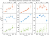	Fig. 5 Similar to Fig. 4 but excluding planetary systems including planets with radii >3.5 R_⊕.
In the text

	Fig. 6 Occurrence rate, F (top), the fraction of stars that host planetary system, η_system (middle), and the average multiplicity, k (bottom) as a function of stellar metallicity [Fe/H] for the sub-Earths from the synthetic population by Bern planet formation and evolution model at 5 Gyr.
In the text

Fig. 7

Period–radius diagram of planets selected from the synthetic population at 2 Gyr after applying the detection selection similar to PAST III (Chen et al. 2022). Planets with different compositions are plotted in different colours: red for H/He-rich envelopes, blue for waterrich envelopes, and green for purely rocky (Silicate+Fe) planets. The dashed lines represent the boundaries of planet radii between different subsamples: Neptune-sized planets, sub-Neptune, valley planet, and super-Earth. Histograms of planetary radius and orbital period are shown in the right panel and the top panel, respectively.

In the text

	Fig. 8 Orbital period-radius diagram of planets with different metallicity [Fe/H] from the synthetic population at 2 Gyr after applying the detection bias similar to PAST III.
In the text

	Fig. 9 Radius distribution of planets with different metallicity [Fe/H] from the synthetic population after applying a detection selection similar to PAST III.
In the text

Fig. 10

Five metrics to characterize the radius valley morphology (i.e. $C_{valley}, A_{valley}, R_{valley}^{+}, R_{valley}^{-}$ $\[C_{\text {valley }}, A_{\text {valley }}, R_{\text {valley }}^{+}, R_{\text {valley }}^{-}\]$ , and f_NP) as functions of [Fe/H] for synthetic population at 2 Gyr after applying the detection bias. The solid lines denote the best fits derived from the synthetic population. The best fits and 1-σ interval derived from the selected observational sample of LAMOST–Gaia–Kepler catalogue (Chen et al. 2021, 2022) are plotted as dashed black lines and grey regions.

In the text

	Fig. 11 Mass-radius distribution of planets with different metallicity [Fe/H] from the synthetic population after applying the detection selection similar to PAST III.
In the text

Fig. 12

Host star metallicities vs. planet orbital period (grey dots) from the synthetic sample. The red line denotes the kernel regression of the mean metallicity of the planet population (from Equation (16)). The shaded red area shows the 68% (1-σ) confidence interval on the mean from bootstrapping. The dashed black line represents the mean metallicity (−0.05 ± 0.04 dex) for stars that host planets with a period >ten days. In the bottom-left corner, we print the Pearson coefficient R between host star metallicity and the orbital periods as well as the correspond p–value.

In the text

	Fig. 13 Similar to Fig. 12 for large planets (top), sub-Neptunes (middle), and terrestrial planets (bottom).
In the text

	Fig. 14 Difference in metallicity between stars hosting planets with orbital period P < 10 and >10 days. The solid red points and error bars show the results derived from the synthetic sample generated by the Bern model. The grey and cyan circles denote the results from Buchhave et al. (2014) and Mulders et al. (2016), respectively.
In the text

	Fig. 15 Planetary occurrence rate as a function of orbital period for super-solar and sub-solar metallicity stars derived from the synthetic population.
In the text

	Fig. 16 Semi-major axis (a) vs. effective mass (M_p sin i) for giant planets in the biased RV synthetic population at 5 Gyr. Solid points and open circles denote planets above and below the detection limit, respectively. The dashed line represents the typical detection limit for corresponding RV surveys when e = 0.
In the text

	Fig. 17 Planetary orbital eccentricity (e) vs. stellar metallicity ([Fe/H]) for giant planets in the synthetic population at 5 Gyr after selection according to the RV detection bias. We also print the Pearson coefficient and corresponding p–value.
In the text

	Fig. 18 Cumulative distributions of stellar metallicities [Fe/H] for high-eccentricity (red) and low-eccentricity giant planets (blue). The two sample KS test p–value is printed in the corner.
In the text

	Fig. 19 Cumulative distributions of stellar metallicities [Fe/H] (top panel) and planetary eccentricity (bottom panel) for single giant planetary systems (blue) and multiple giant planetary systems. The two sample KS test p–values are printed in the lower-right corner of each panel.
In the text

	Fig. 20 Orbital period (P) vs. radius (R_p) for selected small planets in the Kepler-biased synthetic population at 5 Gyr.
In the text

	Fig. 21 Orbital eccentricity vs. stellar metallicity ([Fe/H]) for Kepler-detectable small planets in single (blue) and multiple (orange) systems in the synthetic population. We also plot the mean planetary eccentricity and their 1-σ interval (50 ± 34.1% percentiles) from bootstrapping as solid diamonds and error bars. The best fits are plotted as solid lines.
In the text

Fig. 22

Top: fraction of single transiting small planets with outer giant planets (OGP) vs. stellar metallicities derived from the Kepler-biased synthetic sample. Bottom: Orbital eccentricity vs. stellar metallicity for small transiting planets with and without OGPs (purple/green). The solid lines represent the corresponding best fits. The grey region denotes the 1 − σ interval of the eccentricity-[Fe/H] correlation derived from the LAMOST-Gaia-Kepler sample (An et al. 2023).

In the text

	Fig. 23 Average masses of small planets (regardless of whether they could be detected or not) in single transiting systems without OGPs vs. stellar metallicity (grey circles). The diamonds and error bars denote the mean and 1-σ (50 ± 34.1) interval of the average masses in different bins of [Fe/H]. The solid line represents the best fit.
In the text

Current usage metrics show cumulative count of Article Views (full-text article views including HTML views, PDF and ePub downloads, according to the available data) and Abstracts Views on Vision4Press platform.

Data correspond to usage on the plateform after 2015. The current usage metrics is available 48-96 hours after online publication and is updated daily on week days.

Initial download of the metrics may take a while.

[1] Alibert, Y., Mordasini, C., Benz, W., et al. 2005, A&A, 434, 343 [NASA ADS] [CrossRef] [EDP Sciences] [Google Scholar]

[2] An, D.-S., Xie, J.-W., Dai, Y.-Z., et al. 2023, AJ, 165, 125 [Google Scholar]

[3] Andrews, S. M., Wilner, D. J., Hughes, A. M., et al. 2010, ApJ, 723, 1241 [NASA ADS] [CrossRef] [Google Scholar]

[4] Ayliffe, B. A., & Bate, M. R. 2012, MNRAS, 427, 2597 [Google Scholar]

[5] Baruteau, C., Crida, A., Paardekooper, S.-J., et al. 2014, Protostars and Planets VI, 667 [Google Scholar]

[6] Baruteau, C., & Zhu, Z. 2016, MNRAS, 458, 3927 [NASA ADS] [CrossRef] [Google Scholar]

[7] Bashi D., Mazeh T., & Faigler S., 2024, AJ, 168, 115 [Google Scholar]

[8] Berger, T. A., Huber, D., Gaidos, E., et al. 2020, AJ, 160, 108 [NASA ADS] [CrossRef] [Google Scholar]

[9] Benítez-Llambay, P., Masset, F., & Beaugé, C. 2011, A&A, 528, A2 [NASA ADS] [CrossRef] [EDP Sciences] [Google Scholar]

[10] Bodenheimer, P., & Pollack, J. B. 1986, Icarus, 67, 391 [Google Scholar]

[11] Bodenheimer, P., Hubickyj, O., & Lissauer, J. J. 2000, Icarus, 143, 2 [Google Scholar]

[12] Borucki, W. J., Koch, D., Basri, G., et al. 2010, Science, 327, 977 [Google Scholar]

[13] Buchhave, L. A., Latham, D. W., Johansen, A., et al. 2012, Nature, 486, 375 [NASA ADS] [Google Scholar]

[14] Buchhave, L. A., Bizzarro, M., Latham, D. W., et al. 2014, Nature, 509, 593 [Google Scholar]

[15] Buchhave, L. A., Bitsch, B., Johansen, A., et al. 2018, ApJ, 856, 37 [Google Scholar]

[16] Burn, R., & Mordasini, C. 2024, Handbook of Exoplanets, 2nd edn., eds. H. Deeg & J. Antonio Belmonte (Springer International Publishing), 143-2 [Google Scholar]

[17] Burn, R., Schlecker, M., Mordasini, C., et al. 2021, A&A, 656, A72 [NASA ADS] [CrossRef] [EDP Sciences] [Google Scholar]

[18] Burn, R., Mordasini, C., Mishra, L., et al. 2024a, Nat. Astron., 8, 463 [Google Scholar]

[19] Burn, R., Bali, K., Dorn, C., et al. 2024b, A&A, submitted [arXiv:2411.16879] [Google Scholar]

[20] Butler, R. P., Vogt, S. S., Laughlin, G., et al. 2017, AJ, 153, 208 [Google Scholar]

[21] Chabrier, G., Mazevet, S., & Soubiran, F. 2019, ApJ, 872, 51 [NASA ADS] [CrossRef] [Google Scholar]

[22] Chambers, J. E. 1999, MNRAS, 304, 793 [Google Scholar]

[23] Chambers, J. E. 2001, Icarus, 152, 205 [Google Scholar]

[24] Chambers, J. 2006, Icarus, 180, 496 [NASA ADS] [CrossRef] [Google Scholar]

[25] Chen, D.-C., Yang, J.-Y., Xie, J.-W., et al. 2021, AJ, 162, 100 [NASA ADS] [CrossRef] [Google Scholar]

[26] Chen, D.-C., Xie, J.-W., Zhou, J.-L., et al. 2022, AJ, 163, 249 [NASA ADS] [CrossRef] [Google Scholar]

[27] Chen, D.-C., Xie, J.-W., Zhou, J.-L., et al. 2023, PNAS, 120, e2304179120 [NASA ADS] [CrossRef] [Google Scholar]

[28] Chen, D.-C., Mordasini, C., Xie, J.-W., et al. 2024, A&A, 687, A25 [NASA ADS] [CrossRef] [EDP Sciences] [Google Scholar]

[29] Chen, D.-C., Xie, J.-W., et al. 2025, Nat. Astron., submitted [Google Scholar]

[30] Christian, D. J., Pollacco, D. L., Skillen, I., et al. 2006, MNRAS, 372, 1117 [NASA ADS] [CrossRef] [Google Scholar]

[31] Clarke, C. J., Gendrin, A., & Sotomayor, M. 2001, MNRAS, 328, 485 [NASA ADS] [CrossRef] [Google Scholar]

[32] Coleman, G. A. L., & Nelson, R. P. 2014, MNRAS, 445, 479 [Google Scholar]

[33] Crida, A., Morbidelli, A., & Masset, F. 2006, Icarus, 181, 587 [Google Scholar]

[34] Dawson, R. I., & Johnson, J. A., 2018, ARA&A, 56, 175 [Google Scholar]

[35] Dawson, R. I. & Murray-Clay, R. A., 2013, ApJ, 767, L24 [Google Scholar]

[36] Dittkrist, K.-M., Mordasini, C., Klahr, H., et al. 2014, A&A, 567, A121 [NASA ADS] [CrossRef] [EDP Sciences] [Google Scholar]

[37] Dong, S., Xie, J.-W., Zhou, J.-L., et al. 2018, PNAS, 115, 266 [NASA ADS] [CrossRef] [Google Scholar]

[38] Doyle, L., Armstrong, D. J., Acuña, L., et al. 2025, MNRAS, 539, 3138 [Google Scholar]

[39] Emsenhuber, A., Mordasini, C., Burn, R., et al. 2021a, A&A, 656, A69 [NASA ADS] [CrossRef] [EDP Sciences] [Google Scholar]

[40] Emsenhuber, A., Mordasini, C., Burn, R., et al. 2021b, A&A, 656, A70 [NASA ADS] [CrossRef] [EDP Sciences] [Google Scholar]

[41] Emsenhuber, A., Mordasini, C., & Burn, R. 2023, Eur. Phys. J. Plus, 138, 181 [NASA ADS] [CrossRef] [Google Scholar]

[42] Emsenhuber, A., Mordasini, C., Mayor, M., et al. 2025, A&A, 701, A64 [NASA ADS] [CrossRef] [EDP Sciences] [Google Scholar]

[43] Fabrycky, D., & Tremaine, S. 2007, ApJ, 669, 1298 [NASA ADS] [CrossRef] [Google Scholar]

[44] Fabrycky, D. C., Lissauer, J. J., Ragozzine, D., et al. 2014, ApJ, 790, 146 [Google Scholar]

[45] Ferraz-Mello, S., Rodríguez, A., & Hussmann, H. 2008, Celest. Mech. Dyn. Astron., 101, 171 [Google Scholar]

[46] Fischer, D. A., & Valenti, J. 2005, ApJ, 622, 1102 [NASA ADS] [CrossRef] [Google Scholar]

[47] Fischer, D. A., Marcy, G. W., & Spronck, J. F. P. 2014, ApJS, 210, 5 [Google Scholar]

[48] Fortier, A., Alibert, Y., Carron, F., et al. 2013, A&A, 549, A44 [NASA ADS] [CrossRef] [EDP Sciences] [Google Scholar]

[49] Freedman, R. S., Lustig-Yaeger, J., Fortney, J. J., et al. 2014, ApJS, 214, 25 [CrossRef] [Google Scholar]

[50] Fulton, B. J., Petigura, E. A., Howard, A. W., et al. 2017, AJ, 154, 109 [Google Scholar]

[51] Fűrész, G., Szentgyorgyi, A. H., & Meibom, S. 2008, Precis. Spectrosc. Astrophys., 287 [Google Scholar]

[52] Guo, X., Johnson, J. A., Mann, A. W., et al. 2017, ApJ, 838, 25 [NASA ADS] [CrossRef] [Google Scholar]

[53] Haldemann, J., Alibert, Y., Mordasini, C., et al. 2020, A&A, 643, A105 [NASA ADS] [CrossRef] [EDP Sciences] [Google Scholar]

[54] Hamer, J. H., & Schlaufman, K. C. 2022, AJ, 164, 26 [NASA ADS] [CrossRef] [Google Scholar]

[55] Ho, C. S. K., & Van Eylen, V. 2023, MNRAS, 519, 4056 [NASA ADS] [CrossRef] [Google Scholar]

[56] Ho, C. S. K., Rogers, J. G., Van Eylen, V., Owen, J. E., & Schlichting, H. E. 2024, MNRAS, 531, 3698 [NASA ADS] [CrossRef] [Google Scholar]

[57] Holl, B., Sozzetti, A., Sahlmann, J., et al. 2022, VizieR Online Data Catalog: 367. J/A+A/674/A10 [Google Scholar]

[58] Hsu, D. C., Ford, E. B., Ragozzine, D., et al. 2019, AJ, 158, 109 [NASA ADS] [CrossRef] [Google Scholar]

[59] Huang, C. X., Petrovich, C., & Deibert, E. 2017, AJ, 153, 210 [NASA ADS] [CrossRef] [Google Scholar]

[60] Ida, S., & Lin, D. N. C. 2004, ApJ, 616, 567 [NASA ADS] [CrossRef] [Google Scholar]

[61] Ida, S., & Makino, J. 1993, Icarus, 106, 210 [NASA ADS] [CrossRef] [Google Scholar]

[62] Jackson, B., Greenberg, R., & Barnes, R. 2008, ApJ, 678, 1396 [Google Scholar]

[63] Jackson, B., Barnes, R., & Greenberg, R. 2009, ApJ, 698, 1357 [Google Scholar]

[64] Jin, S., & Mordasini, C. 2018, ApJ, 853, 163 [Google Scholar]

[65] Jin, S., Mordasini, C., Parmentier, V., et al. 2014, ApJ, 795, 65 [Google Scholar]

[66] Johnson, J. A., Aller, K. M., Howard, A. W., et al. 2010, PASP, 122, 905 [Google Scholar]

[67] Johnstone, C. P. 2020, ApJ, 890, 79 [Google Scholar]

[68] Kama, M., Min, M., & Dominik, C. 2009, A&A, 506, 1199 [NASA ADS] [CrossRef] [EDP Sciences] [Google Scholar]

[69] Kite, E. S., Fegley, B., Schaefer, L., et al. 2019, ApJ, 887, L33 [NASA ADS] [CrossRef] [Google Scholar]

[70] Kubyshkina, D. I., & Fossati, L. 2021, RNAAS, 5, 74 [NASA ADS] [Google Scholar]

[71] Kubyshkina, D., Fossati, L., Erkaev, N. V., et al. 2018, A&A, 619, A151 [NASA ADS] [CrossRef] [EDP Sciences] [Google Scholar]

[72] Lai, D., & Pu, B. 2017, AJ, 153, 42 [Google Scholar]

[73] Lai, D. 2012, MNRAS, 423, 486 [NASA ADS] [CrossRef] [Google Scholar]

[74] Lithwick, Y., & Wu, Y. 2011, ApJ, 739, 31 [NASA ADS] [CrossRef] [Google Scholar]

[75] Liu, B., Lambrechts, M., Johansen, A., et al. 2019, A&A, 632, A7 [NASA ADS] [CrossRef] [EDP Sciences] [Google Scholar]

[76] Lodders, K. 2003, ApJ, 591, 1220 [Google Scholar]

[77] Lopez, E. D., & Fortney, J. J. 2013, ApJ, 776, 2 [Google Scholar]

[78] Luque, R., & Pallé, E. 2022, Science, 377, 1211 [NASA ADS] [CrossRef] [Google Scholar]

[79] Lüst, R. 1952, Zeitsch. Naturfor. A, 7, 87 [CrossRef] [Google Scholar]

[80] Lynden-Bell, D., & Pringle, J. E. 1974, MNRAS, 168, 603 [Google Scholar]

[81] Marboeuf, U., Thiabaud, A., Alibert, Y., et al. 2014, A&A, 570, A35 [NASA ADS] [CrossRef] [EDP Sciences] [Google Scholar]

[82] Martinez, C. F., Cunha, K., Ghezzi, L., et al. 2019, ApJ, 875, 29 [CrossRef] [Google Scholar]

[83] Matsuyama, I., Johnstone, D., & Hartmann, L. 2003, ApJ, 582, 893 [NASA ADS] [CrossRef] [Google Scholar]

[84] Mayor, M., Marmier, M., Lovis, C., et al. 2011, arXiv e-prints [arXiv:1109.2497] [Google Scholar]

[85] Mills, S. M., Howard, A. W., Petigura, E. A., et al. 2019, AJ, 157, 198 [Google Scholar]

[86] Mishra, L., Alibert, Y., Leleu, A., et al. 2021, A&A, 656, A74 [NASA ADS] [CrossRef] [EDP Sciences] [Google Scholar]

[87] Mizuno, H. 1980, Progr. Theor. Phys., 64, 544 [CrossRef] [Google Scholar]

[88] Mordasini, C. 2020, A&A, 638, A52 [NASA ADS] [CrossRef] [EDP Sciences] [Google Scholar]

[89] Mordasini, C., Alibert, Y., & Benz, W. 2009a, A&A, 501, 1139 [NASA ADS] [CrossRef] [EDP Sciences] [Google Scholar]

[90] Mordasini, C., Alibert, Y., Benz, W., et al. 2009b, A&A, 501, 1161 [NASA ADS] [CrossRef] [EDP Sciences] [Google Scholar]

[91] Mordasini, C., Alibert, Y., Klahr, H., et al. 2012, A&A, 547, A111 [NASA ADS] [CrossRef] [EDP Sciences] [Google Scholar]

[92] Mordasini, C., Mollière, P., Dittkrist, K.-M., et al. 2015, Int. J. Astrobiol., 14, 201 [NASA ADS] [CrossRef] [Google Scholar]

[93] Moriarty, J., & Ballard, S. 2016, ApJ, 832, 34 [Google Scholar]

[94] Mulders, G. D., Pascucci, I., Apai, D., et al. 2016, AJ, 152, 187 [NASA ADS] [CrossRef] [Google Scholar]

[95] Mulders, G. D. 2018, Handbook of Exoplanets, 153 [Google Scholar]

[96] Mulders, G. D., Mordasini, C., Pascucci, I., et al. 2019, ApJ, 887, 157 [NASA ADS] [CrossRef] [Google Scholar]

[97] Nakamoto, T., & Nakagawa, Y. 1994, ApJ, 421, 640 [Google Scholar]

[98] Neil, A. R., & Rogers, L. A. 2020, ApJ, 891, 12 [Google Scholar]

[99] Ormel, C. W., & Klahr, H. H. 2010, A&A, 520, A43 [NASA ADS] [CrossRef] [EDP Sciences] [Google Scholar]

[100] Owen, J. E., & Wu, Y. 2017, ApJ, 847, 29 [Google Scholar]

[101] Owen, J. E., & Wu, Y. 2013, ApJ, 775, 105 [Google Scholar]

[102] Owen, J. E., & Murray-Clay, R. 2018, MNRAS, 480, 2206 [NASA ADS] [CrossRef] [Google Scholar]

[103] Pan, M., Liu, B., Jiang, L., et al. 2025, ApJ, 985, 1, 7 [Google Scholar]

[104] Perri, F., & Cameron, A. G. W. 1974, Icarus, 22, 416 [Google Scholar]

[105] Petigura, E. A., Marcy, G. W., Winn, J. N., et al. 2018, AJ, 155, 89 [Google Scholar]

[106] Pollack, J. B., Hubickyj, O., Bodenheimer, P., et al. 1996, Icarus, 124, 62 [NASA ADS] [CrossRef] [Google Scholar]

[107] Poon, S. T. S., & Nelson, R. P. 2020, MNRAS, 498, 5166 [NASA ADS] [CrossRef] [Google Scholar]

[108] Pu, B., & Lai, D. 2018, MNRAS, 478, 197 [NASA ADS] [CrossRef] [Google Scholar]

[109] Pu, B., & Wu, Y. 2015, ApJ, 807, 44 [Google Scholar]

[110] Qian, Y., & Wu, Y. 2021, AJ, 161, 201 [NASA ADS] [CrossRef] [Google Scholar]

[111] Raymond, S. N., & Morbidelli, A. 2022, Demographics of Exoplanetary Systems, Lecture Notes of the 3rd Advanced School on Exoplanetary Science, 466, 3 [Google Scholar]

[112] Rafikov, R. R. 2004, AJ, 128, 1348 [NASA ADS] [CrossRef] [Google Scholar]

[113] Ricker, G. R., Winn, J. N., Vanderspek, R., et al. 2015, J. Astron. Telesc. Instrum. Syst., 1, 014003 [Google Scholar]

[114] Santos, N. C., Israelian, G., & Mayor, M. 2001, A&A, 373, 1019 [NASA ADS] [CrossRef] [EDP Sciences] [Google Scholar]

[115] Santos, N. C., Israelian, G., & Mayor, M. 2004, A&A, 415, 1153 [NASA ADS] [CrossRef] [EDP Sciences] [Google Scholar]

[116] Schlecker, M., Mordasini, C., Emsenhuber, A., et al. 2021, A&A, 656, A71 [NASA ADS] [CrossRef] [EDP Sciences] [Google Scholar]

[117] Shakura, N. I., & Sunyaev, R. A. 1973, A&A, 24, 337 [NASA ADS] [Google Scholar]

[118] Shibata, S., Helled, R., & Ikoma, M. 2020, A&A, 633, A33 [NASA ADS] [CrossRef] [EDP Sciences] [Google Scholar]

[119] Telting, J. H., Avila, G., Buchhave, L., et al. 2014, Astron. Nachr., 335, 41 [Google Scholar]

[120] Thiabaud, A., Marboeuf, U., Alibert, Y., et al. 2014, A&A, 562, A27 [NASA ADS] [CrossRef] [EDP Sciences] [Google Scholar]

[121] Thompson, S. E., Coughlin, J. L., Hoffman, K., et al. 2018, ApJS, 235, 38 [NASA ADS] [CrossRef] [Google Scholar]

[122] Thommes, E. W., Duncan, M. J., & Levison, H. F. 2003, Icarus, 161, 431 [NASA ADS] [CrossRef] [Google Scholar]

[123] Trifonov, T., Tal-Or, L., Zechmeister, M., et al. 2020, A&A, 636, A74 [NASA ADS] [CrossRef] [EDP Sciences] [Google Scholar]

[124] Tychoniec, Ł., Tobin, J. J., Karska, A., et al. 2018, ApJS, 238, 19 [Google Scholar]

[125] Udry, S., & Santos, N. C. 2007, ARA&A, 45, 397 [NASA ADS] [CrossRef] [Google Scholar]

[126] Van Eylen, V., & Albrecht, S. 2015, ApJ, 808, 126 [Google Scholar]

[127] Van Eylen, V., Agentoft, C., Lundkvist, M. S., et al. 2018, MNRAS, 479, 4786 [Google Scholar]

[128] Venturini J., Guilera O. M., Haldemann J., Ronco M. P., & Mordasini C., 2020, A&A, 643, L1 [NASA ADS] [CrossRef] [EDP Sciences] [Google Scholar]

[129] Venturini, J., Ronco, M. P., Guilera, O. M., et al. 2024, A&A, 686, L9 [NASA ADS] [CrossRef] [EDP Sciences] [Google Scholar]

[130] Venuti, L., Bouvier, J., Cody, A. M., et al. 2017, A&A, 599, A23 [NASA ADS] [CrossRef] [EDP Sciences] [Google Scholar]

[131] Vissapragada, S., & Behmard, A. 2025, AJ, 169, 2, 117 [Google Scholar]

[132] Wang, J., & Fischer, D. A. 2015, AJ, 149, 14 [NASA ADS] [CrossRef] [Google Scholar]

[133] Weiss, L. M., Marcy, G. W., Petigura, E. A., et al. 2018, AJ, 155, 48 [Google Scholar]

[134] Xie, J.-W., Dong, S., Zhu, Z., et al. 2016, PNAS, 113, 11431 [NASA ADS] [CrossRef] [Google Scholar]

[135] Yang, J.-Y., Xie, J.-W., & Zhou, J.-L. 2020, AJ, 159, 164 [NASA ADS] [CrossRef] [Google Scholar]

[136] Yang, J.-Y., Chen, D.-C., Xie, J.-W., et al. 2023, AJ, 166, 243 [Google Scholar]

[137] Yee, S. W., & Winn, J. N. 2023, ApJ, 949, L21 [CrossRef] [Google Scholar]

[138] Zhou, J.-L., Lin, D. N. C., & Sun, Y.-S. 2007, ApJ, 666, 423 [Google Scholar]

[139] Zhu, W. 2019, ApJ, 873, 8 [NASA ADS] [CrossRef] [Google Scholar]