| Issue |
A&A
Volume 701, September 2025
|
|
|---|---|---|
| Article Number | A79 | |
| Number of page(s) | 19 | |
| Section | Planets, planetary systems, and small bodies | |
| DOI | https://doi.org/10.1051/0004-6361/202555523 | |
| Published online | 04 September 2025 | |
The Hot-Neptune Initiative (HONEI)
I. Two hot sub-Neptunes on a close-in eccentric orbit (TOI-5800 b) and a farther-out circular orbit (TOI-5817 b)
1
INAF – Osservatorio Astrofisico di Torino,
Via Osservatorio 20,
10025
Pino Torinese,
Italy
2
Carnegie Science Observatories,
813 Santa Barbara Street,
Pasadena,
CA
91101,
USA
3
Institute for Particle Physics and Astrophysics,
ETH Zürich, Otto-Stern-Weg 5,
8093
Zürich,
Switzerland
4
INAF – Osservatorio Astronomico di Roma,
Monte P. Catone,
Italy
5
Department of Physics, University of Rome “Tor Vergata”,
Via della Ricerca Scientifica 1,
00133
Rome,
Italy
6
La Sapienza University of Rome, Department of Physics,
Piazzale Aldo Moro 2,
00185
Rome,
Italy
7
INAF – Osservatorio Astronomico di Padova,
Vicolo dell’Osservatorio 5,
35122
Padova,
Italy
8
Fulbright Visiting Research Scholar, Dept. of Astronomy, The University of Texas at Austin,
Speedway 2515,
Austin,
TX,
USA
9
Max-Planck-Institut für Astronomie,
Heidelberg,
Germany
10
INAF – Osservatorio Astrofisico di Catania,
Via S. Sofia 78,
95123
Catania,
Italy
11
Center for Astrophysics | Harvard & Smithsonian,
60 Garden Street,
Cambridge,
MA
02138,
USA
12
Institut d’astrophysique de Paris, UMR7095 CNRS, Université Pierre & Marie Curie,
98bis boulevard Arago,
75014
Paris,
France
13
Observatoire de Haute-Provence, CNRS, Université d’Aix-Marseille,
04870
Saint-Michel-l’Observatoire,
France
14
NASA Ames Research Center,
Moffett Field,
CA
94035,
USA
15
NASA Exoplanet Science Institute, IPAC, California Institute of Technology,
Pasadena,
CA
91125,
USA
16
Centro di Ateneo di Studi e Attività Spaziali “G. Colombo” – Università di Padova,
Via Venezia 15,
35131
Padova,
Italy
17
Physics Department, Austin College,
Sherman,
TX
75090,
USA
18
Observatoire Astronomique de l’Université de Genéve,
Chemin Pegasi 51,
Versoix
1290,
Switzerland
19
DTU Space, Technical University of Denmark,
Elektrovej 328,
DK-2800 Kgs.
Lyngby,
Denmark
20
Fundación Galileo Galilei – INAF,
Rambla José Ana Fernandez Pérez 7,
38712
Breña Baja,
TF,
Spain
21
Université Grenoble Alpes, CNRS, IPAG,
38000
Grenoble,
France
22
Bay Area Environmental Research Institute,
Moffett Field,
CA
94035,
USA
23
Space Telescope Science Institute,
3700 San Martin Drive,
Baltimore,
MD
21218,
USA
24
Dipartimento di Fisica e Astronomia “Galileo Galilei”, Università di Padova,
Vicolo dell’Osservatorio 3,
35122
Padova,
Italy
25
Società Astronomica Lunae, Castelnuovo Magra,
Italy
26
Dept. of Physics, Engineering and Astronomy, Stephen F. Austin State University,
1936 North St,
Nacogdoches,
TX
75962,
USA
★ Corresponding author: This email address is being protected from spambots. You need JavaScript enabled to view it.
Received:
15
May
2025
Accepted:
28
July
2025
Abstract
Context. Neptune-sized exoplanets are key targets for atmospheric studies, yet their formation and evolution remain poorly understood due to their diverse characteristics and limited sample size. The so-called Neptune desert, a region of parameter space with a dearth of short-period sub- to super-Neptunes, is a critical testbed for theories of atmospheric escape and migration.
Aims. The HONEI programme aims to confirm and characterise the best Neptune-sized candidates for composition, atmospheric, and population studies. By measuring planetary masses with high precision, we want to provide the community with optimal targets whose atmosphere can be effectively explored with the James Webb Space Telescope or by ground-based high-resolution spectroscopy.
Methods. For this purpose, we started a radial velocity follow-up campaign, using the twin high-precision spectrographs HARPS and HARPS-N to measure the masses of TESS Neptune-sized candidates and confirm their planetary nature.
Results. In this first paper of the series, we confirm the planetary nature of two candidates: TOI-5800 b and TOI-5817 b. TOI-5800 b is a hot sub-Neptune (Rp = 2.46−0.16+0.18 R⊕, Mp = 9.5−1.9+1.7 M⊕, ρ = 3.46−0.90+1.02 g cm−3, Teq = 1108 ± 20 K) located at the lower edges of the Neptune desert (P = 2.628 days) and is the most eccentric planet (e ~ 0.3) ever found with P < 3 d. TOI-5800 b is expected to still be in the tidal migration phase with its parent star, a K3 V dwarf (V = 9.6 mag), although its eccentricity could arise from interactions with another object in the system. Having a high transmission spectroscopy metric (TSM = 103−22+35), it represents a prime target for future atmospheric characterisation. TOI-5817 b is a relatively hot sub-Neptune (Rp = 3.08 ± 0.14 R⊕, Mp = 10.3−1.3+1.4 M⊕, ρ = 1.93−0.34+0.41 g cm−3, Teq = 950−18+21 K) located in the Neptune savanna (P = 15.610 d), on a circular orbit around a bright G2 IV-V star (V = 8.7 mag). Despite a lower TSM = 56−9+11, it is a potential target for atmospheric follow-up in the context of sub-Neptunes with P > 15 days. Finally, we find that if the difference in the planet densities are mainly due to different gas mass fractions, there will be an order of magnitude difference in the predicted atmospheric carbon-to-oxygen ratios, a prediction that can be tested with atmospheric follow-up observations.
Key words: planets and satellites: dynamical evolution and stability / planets and satellites: fundamental parameters / planets and satellites: interiors / stars: individual: TOI-5800 / stars: individual: TOI-5817
© The Authors 2025
 Open Access article, published by EDP Sciences, under the terms of the Creative Commons Attribution License (https://creativecommons.org/licenses/by/4.0), which permits unrestricted use, distribution, and reproduction in any medium, provided the original work is properly cited.
This article is published in open access under the Subscribe to Open model. This email address is being protected from spambots. You need JavaScript enabled to view it. to support open access publication.
1 Introduction
Neptune-sized exoplanets (3 R⊕ ≲ Rp ≲ 7 R⊕) are unique probes of planetary evolution. Planets in this size range appear to belong to one of three populations, with relatively clear distinctions in system properties, depending on their orbital periods:
Short-period (P ≲ 3 d) Neptunes are rare, resulting in a pronounced ‘Neptune desert’ in the planetary Rp–P and Mp–P planes (Latham et al. 2011; Szabó & Kiss 2011; Lundkvist et al. 2016; Mazeh et al. 2016). This is attributed to both photo-evaporative mass loss and dynamical migration (Matsakos & Königl 2016; Owen & Lai 2018; Vissapragada et al. 2022). Planets in the Neptune desert tend to orbit metal-rich stars (Vissapragada & Behmard 2025; Doyle et al. 2025) and to be exceptionally dense, with extreme examples, such as TOI-849 b, TOI-332 b, and TOI-1853 b, reaching ρ ~ 10 g cm−3 (Armstrong et al. 2020; Osborn et al. 2023; Naponiello et al. 2023).
Between 3 d ≲ P ≲ 6 d the occurrence of these planets sharply peaks in a ‘Neptune ridge’ (Castro-González et al. 2024a), somewhat analogous to the ‘three-day pileup’ of hot Jupiters (Dawson & Johnson 2018). Planets in the Neptune ridge also tend to orbit metal-rich stars (Dong et al. 2018; Petigura et al. 2018, 2022; Vissapragada & Behmard 2025) but with more modest densities, ρ ≲ 2 g cm−3 (Castro-González et al. 2024b), greater eccentricities (i.e. not fully damped by tides; Correia et al. 2020), and misaligned orbits with respect to the stellar spin axis (Bourrier et al. 2023).
For P ≳ 6 d the occurrence flattens off into the ‘Neptune savanna’ (Bourrier et al. 2023; Castro-González et al. 2024a), where planets do not exhibit a host star metallicity preference (Dong et al. 2018; Petigura et al. 2018; Dai et al. 2021; Vissapragada & Behmard 2025), have relatively low eccentricities (Correia et al. 2020), and have even lower densities than the ridge planets, i.e. ρ ≲ 1 g cm−3 (Castro-González et al. 2024b).
These sharp distinctions in occurrence and physical, orbital properties are suggestive of specific evolutionary histories, making Neptunes highly compelling targets for atmospheric characterisation. One hypothesis is that the savanna planets formed relatively close to their current positions and/or experienced a relatively quiescent disc-driven migration, whereas ridge and desert planets are the product of high-eccentricity migration, with the desert planets suffering catastrophic envelope loss in this process (Bourrier et al. 2018; Vissapragada & Behmard 2025). If this is true, planets in the desert, ridge, and savanna should have distinct atmospheric abundances reflecting their divergent evolutionary trajectories (Öberg et al. 2011; Madhusudhan et al. 2017; Booth et al. 2017; Reggiani et al. 2022; Penzlin et al. 2024; Kempton & Knutson 2024; Kirk et al. 2025).
To expand the sample of planets with strong predicted atmospheric signals in order to test atmospheric difference hypotheses, we recently launched the Hot Neptune Initiative (HONEI), which aims to confirm Neptune-sized candidates suitable for atmospheric observations. The selection of the targets for HONEI was based on the full list of TESS objects of interest (TOIs) with estimated sizes of 3 R⊕ ≤ Rp ≤ 7 R⊕ within 1σ uncertainties on Rp. Our size range of interest includes some planets with a radius smaller than that of Neptune, as some of these can have masses greatly exceeding that of Neptune (similar to the dense planets found in the Neptune desert; Armstrong et al. 2020; Osborn et al. 2023; Naponiello et al. 2023). We restricted our mass measurement follow-up efforts to targets with transmission spectroscopy metric (TSM; Kempton et al. 2018) values greater than 701 and orbiting bright stars (J < 11 mag), as these are the best targets for follow-up observations with the spectrographs aboard the James Webb Space Telescope (JWST) and ground-based high-resolution spectrographs such as CRIRES+ and WINERED (Dorn et al. 2023; Otsubo et al. 2024). We vetted all light curves to remove likely false positives and decided to only pursue targets that had been cleared for precision radial velocity (RV) work by small-aperture telescopes. For targets that pass all of these criteria, our aim is to measure the planetary masses with precision better than 20%, as this is required for precise constraints on atmospheric parameters (Batalha et al. 2019) and internal composition models (Dorn et al. 2017).
In this paper we report the first results from the HONEI programme, confirming the two smallest planets in our target list: a sub-Neptune orbiting TOI-5800 and another sub-Neptune around TOI-5817. Both candidate planets had estimated sizes of 3 R⊕ ≤ Rp ≤ 7 R⊕ (within 1σ uncertainties on Rp) and estimated TSM > 70 at the beginning of the programme, although we found that TOI-5800 b is somewhat smaller (![Mathematical equation: $\[2.44_{-0.20}^{+0.29}\]$](/articles/aa/full_html/2025/09/aa55523-25/aa55523-25-eq9.png) R⊕) and TOI-5817 b has a somewhat lower TSM (
R⊕) and TOI-5817 b has a somewhat lower TSM (![Mathematical equation: $\[56_{-9}^{+11}\]$](/articles/aa/full_html/2025/09/aa55523-25/aa55523-25-eq10.png) ). The structure of the paper is as follows. In Sect. 2, we present the TESS and all the ground-based observations we have collected. Section 3 details the characterisation of the two stars and their planets. In Sect. 4, we discuss the properties of the systems and, finally, summarise our conclusions in Sect. 5.
). The structure of the paper is as follows. In Sect. 2, we present the TESS and all the ground-based observations we have collected. Section 3 details the characterisation of the two stars and their planets. In Sect. 4, we discuss the properties of the systems and, finally, summarise our conclusions in Sect. 5.
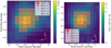 |
Fig. 1 Target pixel file from the TESS observation of Sectors 54 and 55, centred respectively on TOI-5800 (left) and TOI-5817 (right). The SPOC pipeline aperture is shown by shaded red squares. Both fields appear to be uncontaminated by stars within 6 Gaia magnitudes, according to the Gaia DR3 catalogue (Gaia Collaboration 2023). |
2 Observations and data reduction
2.1 TESS photometry
TOI-5800 (also known as HD 193396) and TOI-5817 (also known as HD 204660) have been observed by TESS, respectively, in Sectors 54, 81, 92 (in July–August 2022, August 2024, and May 2025) for a total of 23 transits, and in Sectors 55, 82 (in August–September 2022 and 2024) for a total of only 3 transits. For the analysis detailed in Sect. 3.4, we employed the Presearch Data Conditioning Simple Aperture Photometry (PDC-SAP; Stumpe et al. 2012, 2014, Smith et al. 2012) 2-minute cadence (Sectors 54, 55, 82) and 20-second cadence (Sectors 81, 92) photometry, which are provided by the TESS Science Processing Operations Center (SPOC; Jenkins et al. 2016) pipeline and retrieved via the Python package lightkurve (Lightkurve Collaboration 2018) from the Mikulski Archive for Space Telescopes2. As no other star within 6 magnitudes of the target stars is present in both apertures (see Fig. 1), the dilution coefficients for these light curves are negligible, though the PDC-SAP has already been corrected for dilution3. Both light curves, along with the transits of the candidates TOI-5800.01 and TOI-5817.01, are plotted in Fig. 2.
2.2 Ground-based photometry
We observed a full transit window of TOI-5800.01 continuously for 299 minutes through the Johnson/Cousins I band on 6 August 2024, from the Adams Observatory at Austin College in Sherman, TX. We used a f/8 Ritchey-Chrétien 0.6 m telescope, which has a focal length of 4880 m and is equipped with an FLI ProLine 4096 × 4096 pixel detector, with a pixel size of 9 μm. Therefore, the plate scale is ![Mathematical equation: $\[0^{\prime\prime}_\cdot38\]$](/articles/aa/full_html/2025/09/aa55523-25/aa55523-25-eq11.png) pixel−1, resulting in a 26′ × 26′ field of view. The differential photometric data were extracted using AstroImageJ (Collins et al. 2017). The TESS Transit Finder, which is a customised version of the Tapir software package (Jensen 2013), was used to schedule our transit observations. We observed another full transit window of TOI5800.01 continuously for 299 minutes in Pan-STARRS zs band on 23 October 2024, from the Las Cumbres Observatory Global Telescope (LCOGT; Brown et al. 2013) 1 m network node at the Teide Observatory, on the island of Tenerife (TEID). The 1 m telescope has a focal length of 8100 mm and is equipped with a 4096 × 4096 SINISTRO camera, with a pixel size of 15 μm. The plate scale is
pixel−1, resulting in a 26′ × 26′ field of view. The differential photometric data were extracted using AstroImageJ (Collins et al. 2017). The TESS Transit Finder, which is a customised version of the Tapir software package (Jensen 2013), was used to schedule our transit observations. We observed another full transit window of TOI5800.01 continuously for 299 minutes in Pan-STARRS zs band on 23 October 2024, from the Las Cumbres Observatory Global Telescope (LCOGT; Brown et al. 2013) 1 m network node at the Teide Observatory, on the island of Tenerife (TEID). The 1 m telescope has a focal length of 8100 mm and is equipped with a 4096 × 4096 SINISTRO camera, with a pixel size of 15 μm. The plate scale is ![Mathematical equation: $\[0^{\prime\prime}_\cdot389\]$](/articles/aa/full_html/2025/09/aa55523-25/aa55523-25-eq12.png) per pixel, also resulting in a 26′ × 26′ field of view. The images were calibrated using the standard LCOGT BANZAI pipeline (McCully et al. 2018) and differential photometric data were extracted using AstroImageJ. We used circular
per pixel, also resulting in a 26′ × 26′ field of view. The images were calibrated using the standard LCOGT BANZAI pipeline (McCully et al. 2018) and differential photometric data were extracted using AstroImageJ. We used circular ![Mathematical equation: $\[7^{\prime\prime}_\cdot8\]$](/articles/aa/full_html/2025/09/aa55523-25/aa55523-25-eq13.png) photometric apertures that excluded all of the flux from the nearest known neighbour in the Gaia DR3 catalogue (Gaia DR3 4216062669395306240), which is
photometric apertures that excluded all of the flux from the nearest known neighbour in the Gaia DR3 catalogue (Gaia DR3 4216062669395306240), which is ![Mathematical equation: $\[12^{\prime\prime}_\cdot2\]$](/articles/aa/full_html/2025/09/aa55523-25/aa55523-25-eq14.png) north of TOI-5800.
north of TOI-5800.
The TOI-5800.01 SPOC pipeline transit depth of 731 ppm is generally too shallow to reliably detect with ground-based observations, so we instead checked for possible nearby eclipsing binaries (NEBs) that could be contaminating the TESS photometric aperture and causing the TESS detection. To account for possible contamination from the wings of neighbouring star point spread functions, we searched for NEBs up to ![Mathematical equation: $\[2^{\prime}_\cdot5\]$](/articles/aa/full_html/2025/09/aa55523-25/aa55523-25-eq15.png) from TOI-5800 in both the Adams Observatory and Las Cumbres Observatory TEID observations. If fully blended in the SPOC aperture, a neighbouring star that is fainter than the target star by 7.9 magnitudes in the TESS band could produce the SPOC-reported flux deficit at mid-transit (assuming a 100% eclipse). To account for possible TESS magnitude uncertainties and possible delta-magnitude differences between the TESS band and both the Pan-STARRS zs and Johnson/Cousins I bands, we included an extra 0.5 magnitudes fainter (down to TESS-band magnitude 16.4). We calculated the RMS of each of the 31 nearby star light curves (binned in 10-minute bins) that meet our search criteria and found that the values are smaller by at least a factor of 5 compared to the required NEB depth in each respective star. We then visually inspected each neighbouring star’s light curve to ensure no obvious eclipse-like signal. Our analysis ruled out an NEB blend as the cause of the TOI-5800.01 detection of the SPOC pipeline in the TESS data.
from TOI-5800 in both the Adams Observatory and Las Cumbres Observatory TEID observations. If fully blended in the SPOC aperture, a neighbouring star that is fainter than the target star by 7.9 magnitudes in the TESS band could produce the SPOC-reported flux deficit at mid-transit (assuming a 100% eclipse). To account for possible TESS magnitude uncertainties and possible delta-magnitude differences between the TESS band and both the Pan-STARRS zs and Johnson/Cousins I bands, we included an extra 0.5 magnitudes fainter (down to TESS-band magnitude 16.4). We calculated the RMS of each of the 31 nearby star light curves (binned in 10-minute bins) that meet our search criteria and found that the values are smaller by at least a factor of 5 compared to the required NEB depth in each respective star. We then visually inspected each neighbouring star’s light curve to ensure no obvious eclipse-like signal. Our analysis ruled out an NEB blend as the cause of the TOI-5800.01 detection of the SPOC pipeline in the TESS data.
Furthermore, we analysed the frequency content of the light curves (g band) taken from the ASAS-SN database4 through generalised Lomb-Scargle (GLS; Zechmeister & Kürster 2009) periodograms. We found no sign of modulation for TOI-5800, while for TOI-5817 we found a significant peak occurring at ~29.7 days, and then a second one in the residuals at ~14.8 d, which do not appear in the time series of other activity diagnostics (see Sects. 3.1 and 3.4), making it unlikely that the signals are stellar in origin. We believe that, being almost coincident with 1× and 0.5× the synodic month, they are due to moonlight contamination.
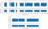 |
Fig. 2 Light curves from the PDC-SAP pipeline of TOI-5800 (top) and TOI-5817 (bottom), as collected by TESS with a 2-minute cadence (or binned to the equivalent of 2 minutes for Sectors 81 and 92). The black line represents our best-fit transit model and detrending (Sect. 3.4); the lower parts of both panels show the residuals of the best-fit model in parts per million. |
2.3 HARPS spectra
Between 30 June 2024 and 13 August 2024, we collected a total of 26 high-resolution spectra of TOI-5800 (Table B.1) with the High Accuracy Radial velocity Planet Searcher (HARPS; Mayor et al. 2003), which is operated at the ESO 3.6 m telescope in the La Silla Observatory (Chile), using exposure times of 15 min. We employed the serval (v.2021-03-31; Zechmeister et al. 2018) and the actin (v.2.0_beta_11; Gomes da Silva et al. 2018) pipelines for the RVs and the stellar activity indices extractions, respectively. In particular, the RV measurements have an average error of 1.46 m s−1, and a median S/N ≈ 41, measured at a reference wavelength of 5500 Å.
2.4 HARPS-N spectra
Between 12 May 2023 and 7 December 2024, we collected a total of 54 high-resolution spectra of TOI-5817 (Table B.2) with the High Accuracy Radial velocity Planet Searcher for the Northern hemisphere (HARPS-N; Cosentino et al. 2012) using an exposure time of 10 min. The first 14 spectra were obtained within the Global Architecture of Planetary Systems (GAPS) Neptune project (Naponiello et al. 2022; Damasso et al. 2023; Naponiello et al. 2025), all the others under the HONEI programme. The RVs and activity indices were extracted from HARPS-N spectra, which were reduced using version 3.0.1 of the HARPS-N Data Reduction Software (DRS; Dumusque et al. 2021), available on the Data Analysis Center for Exoplanets (DACE) web platform. Overall, the measurements have an average uncertainty of 1.16 m s−1, and a S/N ≈ 105, measured at a reference wavelength of 5500 Å.
2.5 SOPHIE spectra
SOPHIE is a stabilised échelle spectrograph dedicated to high-precision RV measurements (Perruchot et al. 2008; Bouchy et al. 2009, 2013) mounted at the 1.93-m telescope of the Observatoire de Haute-Provence in France. HD 204660 was part of a volume-limited survey for giant extrasolar planets (see e.g. Hébrard et al. 2016) performed with SOPHIE, before being identified as the TESS transit-host TOI-5817.01. For the observations of TOI-5817, secured in 2010 and 2024, we used its high-resolution mode (resolving power R = 75 000) and fast readout mode. However, a significant SOPHIE upgrade occurred in between (Bouchy et al. 2013), which introduced a significant improvement in the accuracy of the RV measurements, as well as a possible systematic RV offset whose upper limit is of the order of 15 m/s (Hébrard et al. 2016; Demangeon et al. 2021).
As in other studies, we actually consider the two datasets separately: SOPHIE and SOPHIE+, depending on whether the data were secured before or after the improvement, respectively. Removing a few observations with low precision, for TOI-5817 we have a dataset of 11 and 29 measurements with SOPHIE and SOPHIE+, with average uncertainties ~5.5 m s−1 (4.5× that of HARPS-N) and ~3 m s−1 (2.5×), respectively. The RVs were extracted with the SOPHIE pipeline, as presented by Bouchy et al. (2009) and refined by Heidari et al. (2024, 2025). SOPHIE RV measurements are reported in Table B.3, though they were not included in the final analysis of this work because they do not improve the solution.
2.6 High-resolution imaging
As part of the validation and characterisation process for transiting exoplanets, high-resolution imaging is one of the critical assets required. The presence of a close companion star, whether truly bound or line of sight, will provide ‘third-light’ contamination of the observed transit, leading to incorrect derived properties for both the exoplanet and the host star (Ciardi et al. 2015; Furlan & Howell 2017, 2020). In addition, it has been shown that the presence of a close companion dilutes small-planet transits (Rp < 1.2 R⊕) to the point of non-detection, thereby possibly yielding false occurrence rate predictions (Lester et al. 2021). Given that nearly half of FGK stars are in binary or multiple star systems (Matson et al. 2018), high-resolution imaging yields vital information on each discovered exoplanet as well as more global information on exoplanetary formation, dynamics, and evolution (Howell et al. 2021).
2.6.1 Gemini
TOI-5800 was observed on 2 July 2023, using the Zorro speckle instrument on Gemini South (Scott et al. 2021). Zorro provides simultaneous speckle imaging in two bands (562 nm and 832 nm), delivering reconstructed images and high-precision contrast curves that constrain the presence of close companions (Howell et al. 2011). The data were reduced using our standard pipeline (Howell et al. 2011). Figure B.1 presents the 5σ contrast curves from the observations, along with the 832 nm reconstructed speckle image. The contrast limits show that companions brighter than a delta magnitude of 5 at 0.02 arcsec, and up to a delta magnitude of 9 at 1.2 arcsec, are excluded. TOI5800 is thus consistent with being a single star within these detection limits. At the star’s distance of 42.9 pc, the angular resolution corresponds to projected separations ranging from ~0.9 to 51.5 au.
2.6.2 Palomar
Observations of TOI 5817 were made on 30 June 2023 with the PHARO instrument (Hayward et al. 2001) on the Palomar Hale (5 m) behind the P3K natural guide star AO system (Dekany et al. 2013). The pixel scale for PHARO is 0.025″. The Palomar data were collected in a standard 5-point quincunx dither pattern in the Br-γ filter and Hcont filter. The reduced science frames were combined into a single mosaic-ed image with final resolutions of ~0.094″, and ~0.083″, respectively.
The sensitivity of the final combined adaptive optics images were determined by injecting simulated sources azimuthally around the primary target every 20° at separations of integer multiples of the central source’s full width at half maximum (FWHM; Furlan et al. 2017). The brightness of each injected source was scaled until standard aperture photometry detected it with 5σ significance. The final 5σ limit at each separation was determined from the average of all of the determined limits at that separation and the uncertainty on the limit was set by the rms dispersion of the azimuthal slices at a given radial distance.
The nearby stellar companion (TIC 2001155314 = Gaia DR3 1790807028048264448) – located 2.88 ± 0.02″ to the east (84.0° ± 0.1°) – was detected in both near-infrared images, but no additional close-in stars were detected in agreement with the other imaging techniques. The companion is fainter than the primary target by ΔHcont = 4.81 ± 0.01 mag and ΔBrγ = 4.64 ± 0.02 mag (see Fig. B.3).
2.6.3 SOAR
We also searched for stellar companions to TOI-5817 with speckle imaging on the 4.1 m Southern Astrophysical Research (SOAR) telescope (Tokovinin 2018) on 4 November 2022 UT, observing in the Cousins I band, a similar visible bandpass as TESS. This observation was sensitive with 5σ detection to a 5.2-magnitude fainter star at an angular distance of 1 arcsec from the target. More details of the observations within the SOAR TESS survey are available in Ziegler et al. 2020. The 5σ detection sensitivity and speckle auto-correlation functions from the observations are shown in Fig. B.2.
No nearby stars were firmly detected within 3″ of TOI-5817 in the SOAR observations. In particular, the 2.8″ separated companion resolved by infrared observing Palomar adaptive optics was not detected, despite delta-magnitude sensitivity limits in that separation range of approximately 6.8 magnitudes. This is consistent with a bound late-type companion star, which would be significantly fainter compared to the primary star in the visible pass band of the speckle observation.
3 Analysis
3.1 Host-star characterisations
Stellar atmospheric parameters, including effective temperature (Teff), surface gravity (log g), microturbulence velocity (ξ), and iron abundance ([Fe/H]), were derived using the Python wrapper pyMOOGi (Adamow 2017) for the MOOG code (Sneden 1973). We utilised MARCS plane-parallel model atmospheres (Gustafsson et al. 2008) along with the line lists taken from D’Orazi et al. (2020) and Biazzo et al. (2022). The equivalent widths of the iron lines were measured using ARES (Sousa et al. 2015) and subsequently inputted into the MOOG driver (abfind) to obtain abundances through force fitting. The effective temperature was determined by minimising the slope between the excitation potential of FeI lines and the corresponding abundances, while the microturbulence was refined by minimising the slope between abundances and reduced equivalent widths. Surface gravity was established by enforcing the ionisation equilibrium and ensuring that the average abundance derived from FeI lines equaled that from FeII lines within a tolerance of 0.05 dex. To quantify uncertainties, we considered errors associated with the slopes mentioned above, which contributed to uncertainties in Teff and ξ. For surface gravity, uncertainties were assessed by adjusting log g until the ionisation equilibrium condition was no longer satisfied, resulting in an abundance difference greater than 0.05 dex. We refer the reader to our previous publications for further details (e.g. D’Orazi et al. 2020; Biazzo et al. 2022). Taking into account the same line lists, codes, and grids of models mentioned above, we also measured the elemental abundances of two refractory elements (i.e. magnesium and silicon). The final values are reported in Table 1 and highlight a slight overabundance of the elemental ratios [Mg/Fe] and [Si/Fe].
After deriving the stellar atmospheric parameters, we used the EXOFASTv2 tool (Eastman 2017; Eastman et al. 2019) to determine the stellar mass, radius, and age in a differential evolution Markov chain Monte Carlo Bayesian framework, by imposing Gaussian priors on Teff, [Fe/H], and the Gaia DR3 parallax. Specifically, we simultaneously modelled the spectral energy distribution (SED) of the two host stars and the MESA Isochrones and Stellar Tracks (MIST; Paxton et al. 2015; see Eastman et al. 2019 and Naponiello et al. 2025 for more details). To sample the SED, we used the available Tycho-2 BT and VT, 2MASS J, H, and Ks, and WISE W1, W2, W3, and W4 magnitudes for both stars, and the APASS Johnson B magnitude for TOI-5800 only (see Table 1). The SEDs of both TOI-5800 and TOI-5817 are shown in Fig. B.4 together with their best fit. We found M⋆ = ![Mathematical equation: $\[0.778_{-0.032}^{+0.037}\]$](/articles/aa/full_html/2025/09/aa55523-25/aa55523-25-eq16.png) M⊙, R⋆ = 0.773 ± 0.023 R⊙, and age t =
M⊙, R⋆ = 0.773 ± 0.023 R⊙, and age t = ![Mathematical equation: $\[8.1_{-4.8}^{+4.0}\]$](/articles/aa/full_html/2025/09/aa55523-25/aa55523-25-eq17.png) Gyr for TOI-5800, and M⋆ =
Gyr for TOI-5800, and M⋆ = ![Mathematical equation: $\[0.970_{-0.055}^{+0.072}\]$](/articles/aa/full_html/2025/09/aa55523-25/aa55523-25-eq18.png) M⊙, R⋆ =
M⊙, R⋆ = ![Mathematical equation: $\[1.427_{-0.040}^{+0.043}\]$](/articles/aa/full_html/2025/09/aa55523-25/aa55523-25-eq19.png) R⊙, and age t =
R⊙, and age t = ![Mathematical equation: $\[9.7_{-2.5}^{+2.3}\]$](/articles/aa/full_html/2025/09/aa55523-25/aa55523-25-eq20.png) Gyr for TOI-5817 (see Table 1).
Gyr for TOI-5817 (see Table 1).
3.2 Alternative estimation of TOI-5800’s age
While the advanced age of TOI-5817 is well constrained and consistent with the star being almost on the verge of leaving the main sequence (log g⋆ = 4.15 ± 0.05 is lower than solar gravity log g⊙ = 4.44, even though M⋆ ~ 1 M⊙), the age of TOI-5800 is practically unconstrained from the MIST tracks, as expected for K dwarfs, owing to their slow evolution while on the main sequence. However, even though we keep the value retrieved in Sect. 3.1 as a final estimation, we can also use the chromospheric index (![Mathematical equation: $\[R_{\mathrm{HK}}^{\prime}\]$](/articles/aa/full_html/2025/09/aa55523-25/aa55523-25-eq21.png) ) to make an alternative estimation of TOI-5800 age. According to Eq. (3) of Mamajek & Hillenbrand (2008), we obtain ~4.5 ± 2.0 Gyr, where the uncertainty is evaluated by considering a semi-amplitude for the variation in the chromospheric index Δ log
) to make an alternative estimation of TOI-5800 age. According to Eq. (3) of Mamajek & Hillenbrand (2008), we obtain ~4.5 ± 2.0 Gyr, where the uncertainty is evaluated by considering a semi-amplitude for the variation in the chromospheric index Δ log ![Mathematical equation: $\[R_{\mathrm{HK}}^{\prime}\]$](/articles/aa/full_html/2025/09/aa55523-25/aa55523-25-eq22.png) = ± 0.125 along the activity cycle, a value based on the observed variation along the solar cycle. Moreover, the chromospheric index allows us to estimate the Rossby number Ro of TOI-5800 according to Eq. (5) of Mamajek & Hillenbrand (2008) that gives Ro ~ 1.9. Using the convective turnover time given by Eq. (4) of Noyes et al. (1984), we estimate a rotation period Prot ~ 42 ± 9 days for TOI-5800, where the uncertainty comes from the assumed amplitude of the variation in the chromospheric index along an activity cycle. The age estimated from the gyrochronology relationship of Barnes (2007, his Eq. (3)) is 4.45 ± 2.0 Gyr for the above rotation period and uncertainty.
= ± 0.125 along the activity cycle, a value based on the observed variation along the solar cycle. Moreover, the chromospheric index allows us to estimate the Rossby number Ro of TOI-5800 according to Eq. (5) of Mamajek & Hillenbrand (2008) that gives Ro ~ 1.9. Using the convective turnover time given by Eq. (4) of Noyes et al. (1984), we estimate a rotation period Prot ~ 42 ± 9 days for TOI-5800, where the uncertainty comes from the assumed amplitude of the variation in the chromospheric index along an activity cycle. The age estimated from the gyrochronology relationship of Barnes (2007, his Eq. (3)) is 4.45 ± 2.0 Gyr for the above rotation period and uncertainty.
Such an age estimate is consistent with both the projected rotational velocity, v sin i⋆ (Table 1), and the age derived from the kinematics of the star according to the method proposed by Almeida-Fernandes & Rocha-Pinto (2018). Specifically, it gives an expected age of 3.7 ± 3.0 Gyr using the spatial velocity components of TOI-5800 that we found to be U = −25.0 ± 0.3, V = −24.6 ± 0.2, and W = −0.53 ± 0.15 km s−1 computed with the method of Johnson & Soderblom (1987) with U positive towards the Galactic centre.
Stellar parameters of TOI-5800 and TOI-5817.
3.3 Stellar multiplicity
While for TOI-5800 we do not detect any stellar companion, TOI-5817 has a stellar companion, as detected in the infrared imaging, which is separated by 2.88″ ± 0.02″ at a position angle of 84.0° ± 0.1°. Because of the brightness of the primary target (K2MASS = 7.08 mag), the companion star is undetected in the 2MASS survey but has been resolved by Gaia in both DR2 and DR3, with ΔG = 6.8 mag. De-blending the 2MASS H- and K-band magnitudes, the companion star has real apparent magnitudes of H2MASS = 12.01 ± 0.05 mag and Ks, 2MASS = 11.74 ± 0.05 mag, corresponding to an H − Ks = 0.27 ± 0.07 mag. The companion star has the same parallax (within 1σ) of the primary target. Despite the highly significant difference in the declination component of proper motion, the standard requirement that the scalar proper motion difference is within 10% of the total proper motion (Δμ < 0.1μ; see e.g. Smart et al. 2019) remains satisfied, clearing any doubts on the boundedness of the system. These objects also appear in the Gaia wide binary catalogue by El-Badry et al. (2021). The infrared magnitudes and colours of the companion star are consistent with those of an M3.5V dwarf (Pecaut & Mamajek 2013) separated by approximately 230 au (corresponding to an orbital period much longer than our observational baseline, which makes its RV signal hardly detectable).
Close binary system (separation <1000 au) provide key tests for planet formation models due to the influence of the companion star on the protoplanetary disc. The gravitational pull of the secondary star truncates the disc, reducing its mass and lifetime (Artymowicz & Lubow 1994; Zagaria et al. 2021), which limits material available for planet formation. These conditions can significantly alter the formation and evolution of planets compared to single-star systems (Kraus et al. 2016; Hirsch et al. 2021), by shortening the timescale for gas accretion, reducing solid mass budgets, and changing the distribution of solids, potentially suppressing the formation of sub-Neptunes (Kraus et al. 2012; Moe & Kratter 2021).
3.4 Transit and RV combined fit
For both datasets, we first computed the GLS periodograms of the RVs, using the Python package astropy v.5.2.2 (Price-Whelan et al. 2018), and confirmed that the strongest signals of the respective periodograms are associated with the orbital periods of the candidates (refer to Fig. B.5). Then, we performed a joint transit and RV analysis using the Python wrapper juliet5 (Espinoza et al. 2019), following the same approach of Naponiello et al. (2022). Basically, for the transit-related priors we used the parameters of the data validation report produced by the TESS SPOC pipeline at the NASA Ames Research Center through the Transiting Planet Search (Jenkins 2002; Jenkins et al. 2010, 2020) and data validation (Twicken et al. 2018, Li et al. 2019) modules (Table B.4). Then, we mainly tested two models: one with a fixed eccentricity and another with a uniform distribution of eccentricity values, using the parametrisation ![Mathematical equation: $\[S_{1}= \sqrt{e} \sin~ \omega_{*}, S_{2}=\sqrt{e} \cos~ \omega_{*}\]$](/articles/aa/full_html/2025/09/aa55523-25/aa55523-25-eq30.png) (see Eastman et al. 2013). We also tested models including additional Keplerians with or without linear and parabolic trends, with no meaningful results.
(see Eastman et al. 2013). We also tested models including additional Keplerians with or without linear and parabolic trends, with no meaningful results.
Our analyses clearly confirm the planetary nature of TOI5800 b and TOI-5817 b. The phased models of both the RVs and the transits for each planet are plotted in Figs. 3 and 4, while the RV models of their datasets are displayed in Fig. B.6. As final parameters for the planets (Table 2), we decided to adopt the ones from the eccentric fit for TOI-5800 b and those from the circular fit for TOI-5817 b, because in the first case ![Mathematical equation: $\[\Delta ~\ln~ \mathcal{Z}_{e=0}^{e \geq 0}=3.5\]$](/articles/aa/full_html/2025/09/aa55523-25/aa55523-25-eq31.png) , while in the second
, while in the second ![Mathematical equation: $\[\Delta ~\ln~ \mathcal{Z}_{e=0}^{e \geq 0}=-1.6\]$](/articles/aa/full_html/2025/09/aa55523-25/aa55523-25-eq32.png) , where 𝒵 is the Bayesian evidence of a model fit (note that the threshold for a very strong detection is Δ ln 𝒵 ~ 5, according to Kass & Raftery 1995, while 3 < Δ ln 𝒵 < 5 is considered strong). Indeed, for TOI-5800b the retrieved eccentricity is significant at a ~3.5σ level6 (e =
, where 𝒵 is the Bayesian evidence of a model fit (note that the threshold for a very strong detection is Δ ln 𝒵 ~ 5, according to Kass & Raftery 1995, while 3 < Δ ln 𝒵 < 5 is considered strong). Indeed, for TOI-5800b the retrieved eccentricity is significant at a ~3.5σ level6 (e = ![Mathematical equation: $\[0.300_{-0.082}^{+0.083}\]$](/articles/aa/full_html/2025/09/aa55523-25/aa55523-25-eq33.png) ), while for TOI-5817 b the eccentricity is compatible with zero within ~2σ (e = 0.12 ± 0.07)7. For TOI-5800 b we tested alternative eccentricity priors that favour low values while still allowing a broad range. The inferred eccentricity remained consistent across these choices. We also repeated the analysis using Gaussian processes to model correlated noise, with no significant change in the results.
), while for TOI-5817 b the eccentricity is compatible with zero within ~2σ (e = 0.12 ± 0.07)7. For TOI-5800 b we tested alternative eccentricity priors that favour low values while still allowing a broad range. The inferred eccentricity remained consistent across these choices. We also repeated the analysis using Gaussian processes to model correlated noise, with no significant change in the results.
Furthermore, neither star displays any sign of activity, with no peak in the GLS of the activity indices8 below a false alarm probability (FAP) of 10% (evaluated with the bootstrap method), no sign of significant modulation in the SAP light curve and no significant peak in the GLS of the RV residuals after the removal of the planet signals. This is consistent with both the old ages estimated for the stars and their low values of log ![Mathematical equation: $\[R_{\mathrm{HK}}^{\prime}\]$](/articles/aa/full_html/2025/09/aa55523-25/aa55523-25-eq34.png) (Table 1). We note that there is a small-amplitude, ~5% FAP signal in the residuals of TOI-5800 at ~10 days, which will eventually require more observations to be confirmed. We also verified that there is no discernible modulation in the transit time variations (TTVs) of TOI-5800 b (see Appendix A).
(Table 1). We note that there is a small-amplitude, ~5% FAP signal in the residuals of TOI-5800 at ~10 days, which will eventually require more observations to be confirmed. We also verified that there is no discernible modulation in the transit time variations (TTVs) of TOI-5800 b (see Appendix A).
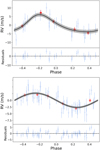 |
Fig. 3 Phased HARPS RVs of TOI-5800 b (top) and phased HARPS-N RVs of TOI-5817 b (bottom) along with the fitted models, in black, and their residuals below each panel. The red circles represent the average of ~5 and ~9 RVs, respectively, while the grey areas represent the 1σ deviation from the model. |
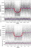 |
Fig. 4 Phase-folded TESS transits of TOI-5800 b (top) and TOI-5817 b (bottom), along with the best-fit models, in red, and the residuals below each panel. The thickness of the red line represents the 1σ spread. The blue circles represent the average of ~8 and ~45 minutes. |
Final parameters from the global fits.
3.5 Detection sensitivities
We estimated the completeness of both the HARPS (TOI5800) and HARPS-N (TOI-5817) RV time series by performing injection-recovery simulations. We injected synthetic RVs with fake planetary signals at the times of our observations, using the original error bars and the estimated stellar jitter (Table 2). We simulated the signals across a logarithmic 30 × 30 grid in planetary mass (Mp) and semi-major axis (a), covering the ranges 0.01–20 MJup (or Jupiter masses) and 0.01–10 au. Similarly to Bonomo et al. (2023), for each location of the grid we generated 200 synthetic planetary signals, drawing a and Mp from a log-uniform distribution inside the cell, T0 from a uniform distribution in [0, P], the orbital inclination i from a uniform cos i distribution in [0, 1], ω* from a uniform distribution in [0, 2π], and e from a beta distribution in [0.0, 0.8] (Kipping 2013). We fitted the signals by employing either Keplerian orbits or linear and quadratic terms, in order to take into account long-period signals, which would not be correctly identified as Keplerian due to the short time span of the RV observations (45 and 575 d, respectively). We then adopted the Bayesian information criterion (BIC) to compare the fitted models with a constant model and considered a planet significantly detected only when ΔBIC > 10 in favour of the planet-induced one. The detection fraction was finally computed as the portion of detected signals for each grid element, as illustrated in Fig. B.7. In particular, we confirm that any Jupiter-mass planet within 1 au and 5 au would have been found around TOI-5800 and TOI-5817, respectively.
In principle, absolute astrometry can provide additional constraints on the presence of orbiting companions. For both stars, the Gaia Data Release 3 (DR3) archive reports values of the re-normalised unit weight error (RUWE), a diagnostic of the departure from a good single-star fit to Gaia-only astrometry, of RUWE = 1.09 and RUWE = 1.11, respectively. These numbers are below the threshold value of 1.4 typically adopted to signify that a single-star model fails to satisfactorily describe the data (e.g. Lindegren et al. 2018, 2021). Using a Monte Carlo simulation to assess the possible companion masses and separations that could result in RUWE values in excess of the ones reported in the Gaia DR3 archive (see Sozzetti 2023 for details) we found that Gaia DR3 astrometry alone can exclude, with 99% confidence, the presence of ~4 and ~13 Jupiter-mass companions within roughly 1–2.5 au around TOI-5800 and TOI-5817, respectively. In the case of TOI-5800, the sensitivity limits from RVs and Gaia DR3 astrometry are comparable, while for TOI-5817 the RVs can rule out the presence of companions over an order of magnitude smaller than Gaia absolute astrometry.
Furthermore, the catalogues of HIPPARCOS-Gaia DR3 astrometric accelerations (Brandt 2021; Kervella et al. 2022) report no statistically significant values of proper motion anomaly for TOI-5817. In the 3–10 au range of orbital separations, which corresponds to the sweet spot of sensitivity for the technique, the HIPPARCOS-Gaia absolute astrometry rules out companions with typical masses above 2.5 MJup (Kervella et al. 2022). Only at around 10 au is this limit comparable to that provided by the RV time-series, which instead typically indicates no planetary companions with masses around 1 MJup or lower are present in the system in the same separation range.
4 Discussion
4.1 Planet interior compositions
Figure 5 shows the mass-radius diagram of small exoplanets with mass and radius determinations better than 4σ and 10σ, respectively, along with the planet iso-composition curves given in Zeng & Sasselov (2013). In this diagram TOI-5800 b is located just below the pure water curve and TOI-5817 b lies above it. This implies that the latter has a considerably higher fraction of volatile elements, as expected from its lower bulk density for a comparable planet mass (Table 2).
To analyse in more detail their composition, we used an inference model based on Dorn et al. (2017) with updates in Luo et al. (2024). The structure model consists of three different layers with an iron core, a silicate mantle, and a volatile layer. The core and mantle are assumed to be adiabatic and can contain both liquid and solid phases. For solid iron we use the equation of state (EOS) for hexagonal close packed iron (Hakim et al. 2018; Miozzi et al. 2020) and for liquid iron and iron alloys we use the EOS by Luo et al. (2024). The mantle is composed of three major species: MgO, SiO2, and FeO. For pressures below ~125 GPa, the solid mantle mineralogy is modelled using the thermodynamical model PERPLE_X (Connolly 2009) and the database from Stixrude & Lithgow-Bertelloni (2022). At higher pressures we define the stable minerals a priori and use their respective EOS from various sources (Hemley et al. 1992; Fischer et al. 2011; Faik et al. 2018; Musella et al. 2019). As there is no data for the density of liquid MgO in the high-pressure temperature regime available, we model the liquid mantle as an ideal mixture of Mg2SiO4, SiO2, and FeO (Melosh 2007; Faik et al. 2018; Ichikawa & Tsuchiya 2020; Stewart et al. 2020). The different components are mixed using the additive volume law.
The volatile layer is modelled as consisting either purely of water or of an uniformly mixed atmosphere of hydrogen, helium, and water. For a pure water layer, the model further takes into account that water can be present in the molten mantle and the iron core (Dorn & Lichtenberg 2021; Luo et al. 2024). The given water mass fraction in the pure water case is thus the accreted bulk water mass fraction and not the mass of the surface water layer.
The outer surface water layer until 0.1 bar is assumed to be isothermal, while, above 0.1 bar, we assume an adiabatic profile. We use the AQUA EOS for water (Haldemann et al. 2020), which covers a large P–T space and water phases. Therefore, our model considers the existences of high-pressure ice shells in the deep layers of the surface water layer. In the case of an uniformly mixed atmosphere, the atmosphere is split into an irradiated outer atmosphere and an inner atmosphere in radiative-convective equilibrium. The atmosphere is modelled using the analytic description of Guillot (2010). The ratio of hydrogen and helium is set to be solar and we use the EOS of Saumon et al. (1995) to describe the H2–He mixture. The water mass fraction of the atmosphere is given by the metallicity Z and described by the ANEOS EOS (Thompson 1990). The two components, H2–He and H2O, are again mixed using the additive volume law.
For the inference, we use a new approach involving surrogate models (paper in prep.), where we use the polynomial chaos Kriging model for surrogate modelling (Schobi et al. 2015; Marelli & Sudret 2014), which approximates the global behaviour of the full physical forward model and replaces it in an Markov chain Monte Carlo framework. The advantage is that the computational costs for a full interior inference is only a few minutes. The prior parameter distribution is listed in Table B.5. We assume that all Si and Mg is in the mantle of the planet. The prior of the Mg/Si mass ratio is thus given by the Mg/Si mass ratio of the host star as measured in this work, which corresponds to 0.91 for TOI-5800 and 0.95 for TOI-5817. The upper bound for the Fe/Si mass ratio in the mantle is given the stellar Fe/Si mass ratio, which is 1.28 for TOI-5800 and 1.31 for TOI-5817. In the pure water case, the upper limit of the bulk water content is set to 0.5 as predicted by planet formation models (e.g. Venturini et al. 2020). For the case of a uniformly mixed atmosphere, the luminosity range is chosen based on the ages of the two systems and the possible atmospheric mass fractions range between 0.1% and 5%. The atmospheric mass fraction refers to the total mass of the atmosphere in H2, He, and H2O. The water mass fraction in the atmosphere is given by the metallicity Z.
The results of the inference model are summarised in Table 3. For both planets a significant amount of volatiles is needed to explain the observed radii given the mass of the two planets. In the case of a H2-He-H2O atmosphere, the atmosphere mass fraction of TOI-5800 b is 1.5% ± 1.0%, while the atmosphere mass fraction of TOI-5817 b is 4.3% ± 0.3%, and neither the metallicity (Z) nor luminosity (L) are well constrained by the data. The ratio of the core-to-mantle mass is roughly Earth-like for both planets. This is mainly constrained by the stellar relative element ratios of Fe, Mg, and Si. Figure B.8 shows the posterior distribution for the case of a uniformly mixed atmosphere for both planets. Nevertheless, we find that both TOI-5800 b and TOI-5817 b can possess atmospheres with super-solar metallicities with Z = 0.43 ± 0.24 and Z = 0.27 ± 0.19, respectively, although metallicity is poorly constrained. This is mainly because we use a uniform prior on Z between 0.02 and 1 and the mass and radius data only carry limited information to put strong constraints on metallicity.
In the hypothetical case of restricting the volatile inventory to water only, the water mass fraction is 16% ± 11% for TOI-5800 b and 31% ± 19% for TOI-5817 b. This extreme scenario informs us on the maximum amount of water possible in the interiors of both worlds. As we take into account any H and O partitioned in the metal core phase, water dissolution in the silicate mantle and the water in a steam envelope, the inferred amount of water represents the maximum amount of accreted water. The inferred values for TOI-5800 b of 16 ± 11% depart significantly from 50% mass fraction, which is generally predicted for worlds that mainly formed outside of the water ice-line and migrated inwards during the gas disc lifetime (Venturini et al. 2020; Burn et al. 2024). Given the water mass fractions of 31 ± 19% for TOI-5817 b, a formation outside of the water ice-line cannot be excluded.
Inferred volatile mass fractions of TOI-5817 b are higher than the one for TOI-5800 b in both scenarios. Compared to the case with a H2-He-H2O atmosphere, the core mass fraction in the pure water case is lower. However, this mass refers only to the mass of the iron core. A significant fraction of the water will be stored in the core as H and O, raising the total core mass.
In order to make a prediction on possible trends of inferred atmospheric C/O ratios from spectroscopy, we employ the model from Schlichting & Young (2022) with recent updates (Werlen et al. 2025). Figure 6 illustrates that an increase in atmospheric mass fraction on top of an Earth-like interior leads to an increase in atmospheric C/O ratios. This can be understood by the fact that the addition of primordial gas leads to a higher production of endogenic water, and water is mainly stored deep in the interior and not in the atmosphere (Luo et al. 2024). As a consequence, a higher atmospheric mass fraction leads to a relative removal of oxygen compared to carbon from the atmosphere. We note that although the trend in atmospheric C/O values holds true, the actual values may vary as we made some assumptions that are poorly constrained by the mass and radius (e.g. bulk O/Si, bulk C/O, and temperature at the magma ocean surface). Overall, if the difference in planet densities between TOI-5800 b and TOI-5817 b are mainly due to a difference in the gas mass fraction, chemical thermodynamics predict a difference in atmospheric C/O ratios of the order of one magnitude; however, we note that the error bars on inferred atmosphere mass fractions are large.
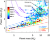 |
Fig. 5 Mass–radius diagram of small (Rp ≤ 4 R⊕) planets, colour-coded by planet equilibrium temperatures. The different solid curves, from bottom to top, correspond to planet compositions of: (i) 100% iron, (ii) 33% iron core and 67% silicate mantle (Earth-like composition); (iii) 100% silicates, (iv) 50% rocky interior and 50% water; and (iv) 100% water, rocky interiors, and (v) 1% or 2% hydrogen-dominated atmospheres (Zeng & Sasselov 2013). The dark grey circles indicate Venus (V), Earth (E), Uranus (U), and Neptune (N). TOI-5800 b and TOI-5817 b are indicated with squares. |
Inference results for the internal compositions of TOI-5800 b and TOI-5817 b.
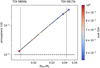 |
Fig. 6 Predicted trend of how atmospheric C/O values change as a function of atmospheric mass assuming a planet mass of 10 M⊕, bulk ratios for C/O = 0.01 (dashed line) and O/Si = 3.3 (Earth-like), and a 3000 K magma ocean surface. Higher atmospheric C/O is predicted for TOI-5817 b than for TOI-5800 b, given their different inferred atmospheric mass fractions (solid grey lines; errors are large and not shown). |
4.2 Tidal effects in the TOI-5800 system
We applied the constant-time lag tidal model by Leconte et al. (2010) to study the tidal evolution of the system. In the case of the Solar System planets Uranus or Neptune, the tidal dissipation is parametrised by the so-called modified tidal quality factor ![Mathematical equation: $\[Q_{\mathrm{p}}^{\prime}\]$](/articles/aa/full_html/2025/09/aa55523-25/aa55523-25-eq77.png) , which is assumed to be of the order of 105 (Ogilvie 2014, Sect. 5.4). Assuming
, which is assumed to be of the order of 105 (Ogilvie 2014, Sect. 5.4). Assuming ![Mathematical equation: $\[Q_{\mathrm{p}}^{\prime}\]$](/articles/aa/full_html/2025/09/aa55523-25/aa55523-25-eq78.png) = 105 for TOI-5800 b and expressing the time lag using Eq. (19) of Leconte et al. (2010), we find an e-folding timescale for the decay of its eccentricity of e/|de/dt| ~ 0.6 Gyr. Therefore, one possibility is that the planet acquired a high-e orbit relatively recently, and we are catching it as it slowly circularises. The circularisation timescale is fairly short compared to the estimated system age (5–10% given the large uncertainties on system age), so catching a planet in this stage should be somewhat rare – and indeed, no other sub-Neptunes with such high-e, short-period orbits are known. Another possibility is that the orbital eccentricity is excited by another body in the system outside our detection limits (Fig. B.7). Such a third body could be a second planet on an eccentric orbit as in the coplanar two-planet system model by Mardling (2007). For example, assuming an outer planet with the same mass of TOI5800 bon a 10-day orbit with an eccentricity of 0.33 (see the end of Sect. 3), the e-folding decay time of the eccentricity of TOI5800 b increases to ~2.9 Gyr, which is comparable with the age of the star derived in Sect. 3.2.
= 105 for TOI-5800 b and expressing the time lag using Eq. (19) of Leconte et al. (2010), we find an e-folding timescale for the decay of its eccentricity of e/|de/dt| ~ 0.6 Gyr. Therefore, one possibility is that the planet acquired a high-e orbit relatively recently, and we are catching it as it slowly circularises. The circularisation timescale is fairly short compared to the estimated system age (5–10% given the large uncertainties on system age), so catching a planet in this stage should be somewhat rare – and indeed, no other sub-Neptunes with such high-e, short-period orbits are known. Another possibility is that the orbital eccentricity is excited by another body in the system outside our detection limits (Fig. B.7). Such a third body could be a second planet on an eccentric orbit as in the coplanar two-planet system model by Mardling (2007). For example, assuming an outer planet with the same mass of TOI5800 bon a 10-day orbit with an eccentricity of 0.33 (see the end of Sect. 3), the e-folding decay time of the eccentricity of TOI5800 b increases to ~2.9 Gyr, which is comparable with the age of the star derived in Sect. 3.2.
We expect significant tidal dissipation in the interior of TOI-5800 b. In fact, with our assumed ![Mathematical equation: $\[Q_{\mathrm{p}}^{\prime}\]$](/articles/aa/full_html/2025/09/aa55523-25/aa55523-25-eq79.png) = 105, the power dissipated inside TOI-5800 b planet is 5.3 × 10¹⁸ W according to Eq. (13) of Leconte et al. (2010). This is already a few percent of the bolometric flux received by the planet (2.7 × 10²⁰ W), and scales with the assumed
= 105, the power dissipated inside TOI-5800 b planet is 5.3 × 10¹⁸ W according to Eq. (13) of Leconte et al. (2010). This is already a few percent of the bolometric flux received by the planet (2.7 × 10²⁰ W), and scales with the assumed ![Mathematical equation: $\[Q_{\mathrm{p}}^{\prime}\]$](/articles/aa/full_html/2025/09/aa55523-25/aa55523-25-eq80.png) . A smaller
. A smaller ![Mathematical equation: $\[Q_{\mathrm{p}}^{\prime}\]$](/articles/aa/full_html/2025/09/aa55523-25/aa55523-25-eq81.png) – for example,
– for example, ![Mathematical equation: $\[Q_{\mathrm{p}}^{\prime}\]$](/articles/aa/full_html/2025/09/aa55523-25/aa55523-25-eq82.png) ~ 104 was recently inferred for WASP-107b (Sing et al. 2024; Welbanks et al. 2024) – would result in even greater dissipation. On the other hand, a higher
~ 104 was recently inferred for WASP-107b (Sing et al. 2024; Welbanks et al. 2024) – would result in even greater dissipation. On the other hand, a higher ![Mathematical equation: $\[Q_{\mathrm{p}}^{\prime}\]$](/articles/aa/full_html/2025/09/aa55523-25/aa55523-25-eq83.png) would result in a longer eccentricity damping timescale. In this case, the observed eccentricity could be a remnant of an initially higher value, and the associated tidal heating would be correspondingly lower. Therefore, depending on the tidal quality factor, intense tidal heating could either significantly affect the planet’s thermal balance (and on the atmospheric chemistry; Fortney et al. 2020) or have a negligible impact.
would result in a longer eccentricity damping timescale. In this case, the observed eccentricity could be a remnant of an initially higher value, and the associated tidal heating would be correspondingly lower. Therefore, depending on the tidal quality factor, intense tidal heating could either significantly affect the planet’s thermal balance (and on the atmospheric chemistry; Fortney et al. 2020) or have a negligible impact.
4.3 Atmospheric characterisation prospects
With TSM = ![Mathematical equation: $\[103_{-22}^{+35}\]$](/articles/aa/full_html/2025/09/aa55523-25/aa55523-25-eq84.png) , TOI-5800 b is an excellent target for atmospheric characterisation with JWST (Kempton et al. 2018). At Teq = 1108 ± 20 K, TOI-5800 b is expected to lack CH4 in chemical equilibrium, making it unlikely to host hydrocarbon hazes (Gao et al. 2020; Brande et al. 2024). Thus, this warm sub-Neptune could be in an aerosol-free regime that makes it ideal for detecting strong atmospheric features, similarly to TOI-421 b (Davenport et al. 2025). Furthermore, if the planetary eccentricity is high because it reached its current position recently and is still tidally circularising, then TOI-5800 b may not have suffered large atmospheric loss, so its composition could be a relatively pristine record of its formation history. Finally, TOI-5800b is one of the top 5 sub-Neptunes for atmospheric spectroscopy orbiting a K dwarf. If strong features are detected in its atmosphere, it could bridge TOI-421 (which orbits a G-type host star and exhibits a low mean-molecular weight atmosphere) and TOI-270 d and GJ9827 d (which exhibit high mean-molecular weight atmospheres and orbit M dwarfs; Benneke et al. 2024; Piaulet-Ghorayeb et al. 2024; Davenport et al. 2025). As for TOI-5817 b, the lower TSM =
, TOI-5800 b is an excellent target for atmospheric characterisation with JWST (Kempton et al. 2018). At Teq = 1108 ± 20 K, TOI-5800 b is expected to lack CH4 in chemical equilibrium, making it unlikely to host hydrocarbon hazes (Gao et al. 2020; Brande et al. 2024). Thus, this warm sub-Neptune could be in an aerosol-free regime that makes it ideal for detecting strong atmospheric features, similarly to TOI-421 b (Davenport et al. 2025). Furthermore, if the planetary eccentricity is high because it reached its current position recently and is still tidally circularising, then TOI-5800 b may not have suffered large atmospheric loss, so its composition could be a relatively pristine record of its formation history. Finally, TOI-5800b is one of the top 5 sub-Neptunes for atmospheric spectroscopy orbiting a K dwarf. If strong features are detected in its atmosphere, it could bridge TOI-421 (which orbits a G-type host star and exhibits a low mean-molecular weight atmosphere) and TOI-270 d and GJ9827 d (which exhibit high mean-molecular weight atmospheres and orbit M dwarfs; Benneke et al. 2024; Piaulet-Ghorayeb et al. 2024; Davenport et al. 2025). As for TOI-5817 b, the lower TSM = ![Mathematical equation: $\[56_{-9}^{+11}\]$](/articles/aa/full_html/2025/09/aa55523-25/aa55523-25-eq85.png) makes it a less favourable target for JWST transmission spectroscopy compared to TOI-5800 b. However, it may still be a good Tier 1 target for Ariel, which promises to deliver lower-resolution spectroscopy for hundreds of sub-Neptunes (Edwards & Tinetti 2022).
makes it a less favourable target for JWST transmission spectroscopy compared to TOI-5800 b. However, it may still be a good Tier 1 target for Ariel, which promises to deliver lower-resolution spectroscopy for hundreds of sub-Neptunes (Edwards & Tinetti 2022).
5 Conclusions
We have confirmed the planetary nature of TOI-5800 b and TOI-5817 b, two hot sub-Neptunes (Teq ~ 1110 K and Teq ~ 950 K) with different orbital periods (P ~ 2.6 d and P ~ 15.6 d) hosted by low-activity K3 V and G2 IV-V stars. In terms of composition, TOI-5800 b can be explained with an Earth-like interior and either a H2-He-H2O atmosphere of ~1 wt% or (as a water world) with a water mass fraction of ~10%. Instead, the lower bulk density of TOI-5817b requires a higher volatile mass fraction and can be explained with an Earth-like interior and a H2-He-H2O atmosphere of ~4 wt% or as a water world with a water mass fraction of ~30%.
In particular, TOI-5800 b is currently undergoing tidal migration, and it stands out as the most eccentric (e ~ 0.3) planet ever found within P < 3 d, with GJ 436b (Lanotte et al. 2014) being a distant second (e ~ 0.15). As it orbits a relatively bright star (VT = 9.7 mag), it is a prime target for atmospheric followup (TSM≳ 100) both with the JWST and from the ground with high-resolution spectroscopy. On the other hand, TOI-5817 b adds to the small but growing sample of well-characterised S-type planets (i.e. it orbits the primary star of a binary system). Studying such planets is essential to testing whether the ‘radius valley’, the observed gap between rocky super-Earths and gas-rich sub-Neptunes (Fulton et al. 2017; Venturini et al. 2020), also applies in binary environments, and how it is shaped by factors such as composition, orbit, and stellar properties. Future atmospheric studies of TOI-5817 b are not out of reach, as it orbits a bright star (VT = 8.7 mag), and they could help constrain the formation and evolution of planets in these dynamically complex systems.
Acknowledgements
We thank S. Jenkins and A. Vanderburg for their collegiality. L.N. acknowledges the financial contribution from the INAF Large Grant 2023 “EXODEMO”. This work has made use of data from the European Space Agency (ESA) mission Gaia (https://www.cosmos.esa.int/gaia), processed by the Gaia Data Processing and Analysis Consortium (DPAC, https://www.cosmos.esa.int/web/gaia/dpac/consortium). Funding for the DPAC has been provided by national institutions, in particular the institutions participating in the Gaia Multilateral Agreement. This work is based on observations collected at the European Southern Observatory under ESO programme(s) 113.26UJ.001, and on observations made with the Italian Telescopio Nazionale Galileo (TNG) operated by the Fundación Galileo Galilei (FGG) of the Istituto Nazionale di Astrofisica (INAF) at the Observatorio del Roque de los Muchachos (La Palma, Canary Islands, Spain). We acknowledge the Italian center for Astronomical Archives (IA2, https://www.ia2.inaf.it), part of the Italian National Institute for Astrophysics (INAF), for providing technical assistance, services and supporting activities of the GAPS collaboration. This work includes data collected with the TESS mission, obtained from the MAST data archive at the Space Telescope Science Institute (STScI). Funding for the TESS mission is provided by the NASA Explorer Program. STScI is operated by the Association of Universities for Research in Astronomy, Inc., under the NASA contract NAS 5–26555. We acknowledge the use of public TESS data from pipelines at the TESS Science Office and at the TESS Science Processing Operations Center. Resources supporting this work were provided by the NASA High-End Computing (HEC) Program through the NASA Advanced Supercomputing (NAS) Division at Ames Research Center for the production of the SPOC data products. This work also includes observations obtained at the Hale Telescope, Palomar Observatory, as part of a collaborative agreement between the Caltech Optical Observatories and the Jet Propulsion Laboratory operated by Caltech for NASA. Funding for the TESS mission is provided by NASA’s Science Mission Directorate. KAC and CNW acknowledge support from the TESS mission via subaward s3449 from MIT. CD acknowledges support from the Swiss National Science Foundation under grant TMSGI2_211313. Parts of this work has been carried out within the framework of the NCCR PlanetS supported by the Swiss National Science Foundation under grants 51NF40_182901 and 51NF40_205606. MP acknowledges support from the European Union – NextGenerationEU (PRIN MUR 2022 20229R43BH) and the “Programma di Ricerca Fondamentale INAF 2023”. TZi acknowledges support from CHEOPS ASI-INAF agreement no. 2019-29-HH.0, NVIDIA Academic Hardware Grant Program for the use of the Titan V GPU card and the Italian MUR Departments of Excellence grant 2023–2027 “Quantum Frontiers”. JJL received support from NASA’s Exoplanet Research Program project 24-XRP24_2-0020. This work makes use of observations from the LCOGT network. Part of the LCOGT telescope time was granted by NOIRLab through the Mid-Scale Innovations Program (MSIP). MSIP is funded by NSF. This research has made use of the Exoplanet Follow-up Observation Program (ExoFOP; DOI: 10.26134/ExoFOP5) website, which is operated by the California Institute of Technology, under contract with the National Aeronautics and Space Administration under the Exoplanet Exploration Program. This work made use of tpfplotter by J. Lillo-Box (publicly available in www.github.com/jlillo/tpfplotter). This work uses observations secured with the SOPHIE spectrograph at the 1.93-m telescope of Observatoire Haute-Provence, France, with the support of its staff. This work was supported by the “Programme National de Planétologie” (PNP) of CNRS/INSU, and CNES. Some of the observations in this paper made use of the High-Resolution Imaging instrument Zorro and were obtained under Gemini LLP Proposal Number: GN/S-2021A-LP-105. Zorro was funded by the NASA Exoplanet Exploration Program and built at the NASA Ames Research Center by Steve B. Howell, Nic Scott, Elliott P. Horch, and Emmett Quigley. Zorro was mounted on the Gemini South telescope of the international Gemini Observatory, a program of NSF’s OIR Lab, which is managed by the Association of Universities for Research in Astronomy (AURA) under a cooperative agreement with the National Science Foundation. on behalf of the Gemini partnership: the National Science Foundation (United States), National Research Council (Canada), Agencia Nacional de Investigación y Desarrollo (Chile), Ministerio de Ciencia, Tecnología e Innovación (Argentina), Ministério da Ciência, Tecnologia, Inovações e Comunicações (Brazil), and Korea Astronomy and Space Science Institute (Republic of Korea). LM acknowledges financial contribution from PRIN MUR 2022 project 2022J4H55R. DRC acknowledges partial support from NASA Grant 18-2XRP18_2-0007.
Appendix A TOI-5800 b TTV analysis
To investigate the presence of TTVs for TOI-5800 b, we performed a dedicated analysis of the TESS photometric time series using juliet, fitting each transit independently. The resulting mid-transit times and their associated uncertainties were compiled into a dataset of transit epochs and corresponding O–C (observed minus calculated) residuals relative to a linear ephemeris. The analysis revealed no statistically significant TTV signal in the observed transits (Fig. A.1, Table A.1). The posterior distributions of the mid-transit times are consistent with white noise dominated deviations, and no apparent periodic structure is evident in the O–C diagram. We conclude that, within the current timing precision and observational baseline, there is no evidence of significant dynamical perturbations in the orbit of TOI-5800 b detectable via TTVs.
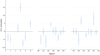 |
Fig. A.1 Observed minus calculated centre times for the transits of TOI5800 b (Sectors 54, 81, and 92). |
TTV values and uncertainties for TOI-5800 b.
Appendix B Additional figures and tables
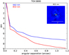 |
Fig. B.1 5σ magnitude contrast curves in both filters as a function of the angular separation out to 1.2 arcsec, as taken by Gemini. The inset shows the reconstructed 832 nm image of TOI-5800 with a 1 arcsec scale bar. TOI-5800 was found to have no close companions from the diffraction limit (0.02”) out to 1.2 arcsec to within the contrast levels achieved. |
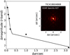 |
Fig. B.2 5σ magnitude contrast curve in the Cousins I band as a function of the angular separation out to 3 arcsec, as taken by SOAR. The inset shows the reconstructed images of TOI-5817 in the same band. No stellar companion to TOI-5817 is seen. |
 |
Fig. B.3 5σ magnitude contrast curves in the Hcont filter (left) and Br-γ filter (right) as a function of the angular separation out to 4 arcsec, as taken by Palomar adaptive optics. The inset shows the reconstructed images of TOI-5817 in the respective filters. A stellar companion of TOI-5817 is clearly spotted, as detailed in Sect. 3.3, though no close-in companions were detected, in agreement with the other speckle imaging performed for TOI-5817 (Fig. B.2). |
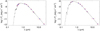 |
Fig. B.4 SEDs of the host stars TOI-5800 (left) and TOI-5817 (right). The broadband measurements from the Tycho, APASS Johnson, 2MASS, and WISE magnitudes are shown in red, and the corresponding theoretical values with blue circles. The un-averaged best-fit model is displayed with a solid black line. |
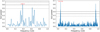 |
Fig. B.5 GLS periodograms of TOI-5800 (left) and TOI-5817 (right) RVs. The horizontal dotted lines mark, respectively, the 0.1%, 1%, and 10% FAP levels from top to bottom. In both cases, the second peak falls precisely at the 1 d alias of the transiting candidate periods (highlighted in red). |
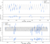 |
Fig. B.6 HARPS RVs of TOI-5800 (top) and HARPS-N RVs of TOI-5817 (bottom) along with the best-fit models, in black, and their residuals below each panel. |
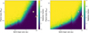 |
Fig. B.7 HARPS and HARPS-N RV detection maps for TOI-5800 (left) and TOI-5817 (right). The colour scale expresses the detection fraction (i.e. the detection probability), while the red circles mark the position of TOI-5800 b (left) and TOI-5817 b (right). Jupiter and Saturn are shown for comparison. |
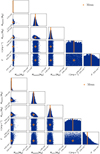 |
Fig. B.8 Posterior distribution for the internal composition analyses of TOI-5800 b (top) and TOI-5817 b (bottom). |
TOI-5800 HARPS RV data points and activity indices.
TOI-5817 HARPS-N RV data points and activity indices.
TOI-5817 SOPHIE and SOPHIE+ RVs, separated by a horizontal line.
Prior parameter distribution for the calculation of the internal compositions of TOI-5800 b and TOI-5817 b.
References
- Adamow, M. M. 2017, in American Astronomical Society Meeting Abstracts, 230, 216.07 [NASA ADS] [Google Scholar]
- Almeida-Fernandes, F., & Rocha-Pinto, H. J. 2018, MNRAS, 476, 184 [Google Scholar]
- Armstrong, D. J., Lopez, T. A., Adibekyan, V., et al. 2020, Nature, 583, 39 [Google Scholar]
- Artymowicz, P., & Lubow, S. H. 1994, ApJ, 421, 651 [Google Scholar]
- Barnes, S. A. 2007, ApJ, 669, 1167 [Google Scholar]
- Batalha, N. E., Lewis, T., Fortney, J. J., et al. 2019, ApJ, 885, L25 [Google Scholar]
- Benneke, B., Roy, P.-A., Coulombe, L.-P., et al. 2024, AAS J., submitted [arXiv:2403.03325] [Google Scholar]
- Biazzo, K., D’Orazi, V., Desidera, S., et al. 2022, A&A, 664, A161 [NASA ADS] [CrossRef] [EDP Sciences] [Google Scholar]
- Bonomo, A. S., Dumusque, X., Massa, A., et al. 2023, A&A, 677, A33 [NASA ADS] [CrossRef] [EDP Sciences] [Google Scholar]
- Booth, R. A., Clarke, C. J., Madhusudhan, N., & Ilee, J. D. 2017, MNRAS, 469, 3994 [Google Scholar]
- Bouchy, F., Hébrard, G., Udry, S., et al. 2009, A&A, 505, 853 [NASA ADS] [CrossRef] [EDP Sciences] [Google Scholar]
- Bouchy, F., Díaz, R. F., Hébrard, G., et al. 2013, A&A, 549, A49 [NASA ADS] [CrossRef] [EDP Sciences] [Google Scholar]
- Bourrier, V., Lovis, C., Beust, H., et al. 2018, Nature, 553, 477 [NASA ADS] [CrossRef] [Google Scholar]
- Bourrier, V., Attia, M., Mallonn, M., et al. 2023, A&A, 669, A63 [NASA ADS] [CrossRef] [EDP Sciences] [Google Scholar]
- Brande, J., Crossfield, I. J. M., Kreidberg, L., et al. 2024, ApJ, 961, L23 [NASA ADS] [CrossRef] [Google Scholar]
- Brandt, T. D. 2021, ApJS, 254, 42 [NASA ADS] [CrossRef] [Google Scholar]
- Brown, T. M., Baliber, N., Bianco, F. B., et al. 2013, PASP, 125, 1031 [Google Scholar]
- Burn, R., Bali, K., Dorn, C., Luque, R., & Grimm, S. L. 2024, A&A, submitted [arXiv:2411.16879] [Google Scholar]
- Cannon, A. J., & Pickering, E. C. 1918 –1924, Annals of H. College Observatory, 91, The Henry Draper Catalogue (Harvard College Observatory) [Google Scholar]
- Castro-González, A., Bourrier, V., Lillo-Box, J., et al. 2024a, A&A, 689, A250 [NASA ADS] [CrossRef] [EDP Sciences] [Google Scholar]
- Castro-González, A., Lillo-Box, J., Armstrong, D. J., et al. 2024b, A&A, 691, A233 [NASA ADS] [CrossRef] [EDP Sciences] [Google Scholar]
- Ciardi, D. R., Beichman, C. A., Horch, E. P., & Howell, S. B. 2015, ApJ, 805, 16 [NASA ADS] [CrossRef] [Google Scholar]
- Collins, K. A., Kielkopf, J. F., Stassun, K. G., & Hessman, F. V. 2017, AJ, 153, 77 [Google Scholar]
- Connolly, J. A. D. 2009, The Geodynamic Equation of State: What and How – Connolly – 2009 – Geochemistry, Geophysics, Wiley Online Library [Google Scholar]
- Correia, A. C. M., Bourrier, V., & Delisle, J. B. 2020, A&A, 635, A37 [NASA ADS] [CrossRef] [EDP Sciences] [Google Scholar]
- Cosentino, R., Lovis, C., Pepe, F., et al. 2012, SPIE Conf. Ser., 8446, 84461V [Google Scholar]
- Cutri, R. M., Skrutskie, M. F., van Dyk, S., et al. 2003, 2MASS All-Sky Catalog of Point Sources, VizieR On-line Data Catalog: II/246. Published in: University of Massachusetts and Infrared Processing and Analysis Center, (IPAC/California Institute of Technology; 2003) [Google Scholar]
- Cutri, R. M., Wright, E. L., Conrow, T., et al. 2021, AllWISE Data Release, VizieR On-line Data Catalog: II/328. Published in: IPAC/Caltech (2013) [Google Scholar]
- Dai, F., Howard, A. W., Batalha, N. M., et al. 2021, AJ, 162, 62 [NASA ADS] [CrossRef] [Google Scholar]
- Damasso, M., Locci, D., Benatti, S., et al. 2023, A&A, 672, A126 [NASA ADS] [CrossRef] [EDP Sciences] [Google Scholar]
- Davenport, B., Kempton, E. M.-R., Nixon, M. C., et al. 2025, ApJ, 984, L44 [Google Scholar]
- Dawson, R. I., & Johnson, J. A. 2018, ARA&A, 56, 175 [Google Scholar]
- Dekany, R., Roberts, J., Burruss, R., et al. 2013, ApJ, 776, 130 [CrossRef] [Google Scholar]
- Demangeon, O. D. S., Dalal, S., Hébrard, G., et al. 2021, A&A, 653, A78 [NASA ADS] [CrossRef] [EDP Sciences] [Google Scholar]
- Dong, S., Xie, J.-W., Zhou, J.-L., Zheng, Z., & Luo, A. 2018, PNAS, 115, 266 [NASA ADS] [CrossRef] [Google Scholar]
- D’Orazi, V., Oliva, E., Bragaglia, A., et al. 2020, A&A, 633, A38 [NASA ADS] [CrossRef] [EDP Sciences] [Google Scholar]
- Dorn, C., & Lichtenberg, T. 2021, ApJ, 922, L4 [NASA ADS] [CrossRef] [Google Scholar]
- Dorn, C., Venturini, J., Khan, A., et al. 2017, A&A, 597, A37 [NASA ADS] [CrossRef] [EDP Sciences] [Google Scholar]
- Dorn, R. J., Bristow, P., Smoker, J. V., et al. 2023, A&A, 671, A24 [NASA ADS] [CrossRef] [EDP Sciences] [Google Scholar]
- Doyle, L., Armstrong, D. J., Acuña, L., et al. 2025, MNRAS, submitted [arXiv:2504.16164] [Google Scholar]
- Dumusque, X., Cretignier, M., Sosnowska, D., et al. 2021, A&A, 648, A103 [NASA ADS] [CrossRef] [EDP Sciences] [Google Scholar]
- Eastman, J. 2017, Astrophysics Source Code Library [record asc1:1710.003] [Google Scholar]
- Eastman, J., Gaudi, B. S., & Agol, E. 2013, PASP, 125, 83 [Google Scholar]
- Eastman, J. D., Rodriguez, J. E., Agol, E., et al. 2019, PASP, submitted [arXiv:1907.09480] [Google Scholar]
- Edwards, B., & Tinetti, G. 2022, AJ, 164, 15 [NASA ADS] [CrossRef] [Google Scholar]
- El-Badry, K., Rix, H.-W., & Heintz, T. M. 2021, MNRAS, 506, 2269 [NASA ADS] [CrossRef] [Google Scholar]
- Espinoza, N., Kossakowski, D., & Brahm, R. 2019, MNRAS, 490, 2262 [Google Scholar]
- Faik, S., Tauschwitz, A., & Iosilevskiy, I. 2018, Comput. Phys. Commun., 227, 117 [NASA ADS] [CrossRef] [Google Scholar]
- Fischer, R. A., Campbell, A. J., Shofner, G. A., et al. 2011, Earth Planet. Sci. Lett., 304, 496 [CrossRef] [Google Scholar]
- Fortney, J. J., Visscher, C., Marley, M. S., et al. 2020, AJ, 160, 288 [NASA ADS] [CrossRef] [Google Scholar]
- Fulton, B. J., Petigura, E. A., Howard, A. W., et al. 2017, AJ, 154, 109 [Google Scholar]
- Furlan, E., & Howell, S. B. 2017, AJ, 154, 66 [NASA ADS] [CrossRef] [Google Scholar]
- Furlan, E., & Howell, S. B. 2020, ApJ, 898, 47 [NASA ADS] [CrossRef] [Google Scholar]
- Furlan, E., Ciardi, D. R., Everett, M. E., et al. 2017, AJ, 153, 71 [NASA ADS] [CrossRef] [Google Scholar]
- Gaia Collaboration (Vallenari, A., et al.) 2023, A&A, 674, A1 [NASA ADS] [CrossRef] [EDP Sciences] [Google Scholar]
- Gao, P., Thorngren, D. P., Lee, E. K. H., et al. 2020, Nat. Astron., 4, 951 [NASA ADS] [CrossRef] [Google Scholar]
- Gomes da Silva, J., Figueira, P., Santos, N., & Faria, J. 2018, J. Open Source Softw., 3, 667 [Google Scholar]
- Guerrero, N. M., Seager, S., Huang, C. X., et al. 2021, ApJS, 254, 39 [NASA ADS] [CrossRef] [Google Scholar]
- Guillot, T. 2010, A&A, 520, A27 [NASA ADS] [CrossRef] [EDP Sciences] [Google Scholar]
- Gustafsson, B., Edvardsson, B., Eriksson, K., et al. 2008, A&A, 486, 951 [NASA ADS] [CrossRef] [EDP Sciences] [Google Scholar]
- Hakim, K., Rivoldini, A., Van Hoolst, T., et al. 2018, Icarus, 313, 61 [Google Scholar]
- Haldemann, J., Alibert, Y., Mordasini, C., & Benz, W. 2020, A&A, 643, A105 [NASA ADS] [CrossRef] [EDP Sciences] [Google Scholar]
- Hayward, T. L., Brandl, B., Pirger, B., et al. 2001, PASP, 113, 105 [NASA ADS] [CrossRef] [Google Scholar]
- Hébrard, G., Arnold, L., Forveille, T., et al. 2016, A&A, 588, A145 [Google Scholar]
- Heidari, N., Boisse, I., Hara, N. C., et al. 2024, A&A, 681, A55 [NASA ADS] [CrossRef] [EDP Sciences] [Google Scholar]
- Heidari, N., Hébrard, G., Martioli, E., et al. 2025, A&A, 694, A36 [NASA ADS] [CrossRef] [EDP Sciences] [Google Scholar]
- Hemley, R. J., Stixrude, L., Fei, Y., & Mao, H. K. 1992, in High-Pressure Research: Application to Earth and Planetary Sciences (American Geophysical Union; AGU), 183 [Google Scholar]
- Henden, A. A., Templeton, M., Terrell, D., et al. 2016, AAVSO Photometric All Sky Survey (APASS) DR9, VizieR On-line Data Catalog: II/336. Published in: 2015AAS...22533616H [Google Scholar]
- Hirsch, L. A., Rosenthal, L., Fulton, B. J., et al. 2021, AJ, 161, 134 [NASA ADS] [CrossRef] [Google Scholar]
- Høg, E., Fabricius, C., Makarov, V. V., et al. 2000, A&A, 355, L27 [Google Scholar]
- Howell, S. B., Everett, M. E., Sherry, W., Horch, E., & Ciardi, D. R. 2011, AJ, 142, 19 [Google Scholar]
- Howell, S. B., Matson, R. A., Ciardi, D. R., et al. 2021, AJ, 161, 164 [NASA ADS] [CrossRef] [Google Scholar]
- Ichikawa, H., & Tsuchiya, T. 2020, Minerals, 10, 59 [CrossRef] [Google Scholar]
- Jenkins, J. M. 2002, ApJ, 575, 493 [Google Scholar]
- Jenkins, J. M., Chandrasekaran, H., McCauliff, S. D., et al. 2010, SPIE Conf. Ser., 7740, 77400D [Google Scholar]
- Jenkins, J. M., Twicken, J. D., McCauliff, S., et al. 2016, SPIE Conf. Ser., 9913, 99133E [Google Scholar]
- Jenkins, J. M., Tenenbaum, P., Seader, S., et al. 2020, Kepler Data Processing Handbook: Transiting Planet Search, Kepler Science Document KSCI-19081-003, 9, ed. J. M. Jenkins [Google Scholar]
- Jensen, E. 2013, Astrophysics Source Code Library [record ascl:1306.007] [Google Scholar]
- Johnson, D. R. H., & Soderblom, D. R. 1987, AJ, 93, 864 [Google Scholar]
- Kass, R. E., & Raftery, A. E. 1995, J. Am. Statist. Assoc., 90, 773 [CrossRef] [Google Scholar]
- Kempton, E. M. R., & Knutson, H. A. 2024, Rev. Mineral. Geochem., 90, 411 [CrossRef] [Google Scholar]
- Kempton, E. M. R., Bean, J. L., Louie, D. R., et al. 2018, PASP, 130, 114401 [Google Scholar]
- Kervella, P., Arenou, F., & Thévenin, F. 2022, A&A, 657, A7 [NASA ADS] [CrossRef] [EDP Sciences] [Google Scholar]
- Kipping, D. M. 2013, MNRAS, 434, L51 [Google Scholar]
- Kirk, J., Ahrer, E.-M., Claringbold, A. B., et al. 2025, MNRAS, submitted [arXiv:2410.08116] [Google Scholar]
- Kochanek, C. S., Shappee, B. J., Stanek, K. Z., et al. 2017, PASP, 129, 104502 [Google Scholar]
- Kraus, A. L., Ireland, M. J., Hillenbrand, L. A., & Martinache, F. 2012, ApJ, 745, 19 [Google Scholar]
- Kraus, A. L., Ireland, M. J., Huber, D., Mann, A. W., & Dupuy, T. J. 2016, AJ, 152, 8 [NASA ADS] [CrossRef] [Google Scholar]
- Lanotte, A. A., Gillon, M., Demory, B. O., et al. 2014, A&A, 572, A73 [NASA ADS] [CrossRef] [EDP Sciences] [Google Scholar]
- Latham, D. W., Rowe, J. F., Quinn, S. N., et al. 2011, ApJ, 732, L24 [NASA ADS] [CrossRef] [Google Scholar]
- Leconte, J., Chabrier, G., Baraffe, I., & Levrard, B. 2010, A&A, 516, A64 [NASA ADS] [CrossRef] [EDP Sciences] [Google Scholar]
- Lester, K. V., Matson, R. A., Howell, S. B., et al. 2021, AJ, 162, 75 [NASA ADS] [CrossRef] [Google Scholar]
- Li, J., Tenenbaum, P., Twicken, J. D., et al. 2019, PASP, 131, 1 [Google Scholar]
- Lightkurve Collaboration (Cardoso, J. V. d. M., et al.) 2018, Astrophysics Source Code Library [record ascl:1812.013] [Google Scholar]
- Lindegren, L., Hernández, J., Bombrun, A., et al. 2018, A&A, 616, A2 [NASA ADS] [CrossRef] [EDP Sciences] [Google Scholar]
- Lindegren, L., Klioner, S. A., Hernández, J., et al. 2021, A&A, 649, A2 [EDP Sciences] [Google Scholar]
- Lundkvist, M. S., Kjeldsen, H., Albrecht, S., et al. 2016, Nat. Commun., 7, 11201 [Google Scholar]
- Luo, H., Dorn, C., & Deng, J. 2024, Nat. Astron., 8, 1399 [Google Scholar]
- Madhusudhan, N., Bitsch, B., Johansen, A., & Eriksson, L. 2017, MNRAS, 469, 4102 [NASA ADS] [CrossRef] [Google Scholar]
- Mamajek, E. E., & Hillenbrand, L. A. 2008, ApJ, 687, 1264 [Google Scholar]
- Mardling, R. A. 2007, MNRAS, 382, 1768 [NASA ADS] [Google Scholar]
- Marelli, S., & Sudret, B. 2014, in Vulnerability, Uncertainty, and Risk (2nd Int. Conf. on Vulnerability, Risk Analysis and Management), 2554 [Google Scholar]
- Matsakos, T., & Königl, A. 2016, ApJ, 820, L8 [Google Scholar]
- Matson, R. A., Howell, S. B., Horch, E. P., & Everett, M. E. 2018, AJ, 156, 31 [NASA ADS] [CrossRef] [Google Scholar]
- Mayor, M., Pepe, F., Queloz, D., et al. 2003, The Messenger, 114, 20 [NASA ADS] [Google Scholar]
- Mazeh, T., Holczer, T., & Faigler, S. 2016, A&A, 589, A75 [NASA ADS] [CrossRef] [EDP Sciences] [Google Scholar]
- McCully, C., Volgenau, N. H., Harbeck, D.-R., et al. 2018, SPIE Conf. Ser., 10707, 107070K [Google Scholar]
- Melosh, H. J. 2007, Meteor. Planet. Sci., 42, 2079 [NASA ADS] [CrossRef] [Google Scholar]
- Miozzi, F., Matas, J., Guignot, N., et al. 2020, Minerals, 10, 100 [CrossRef] [Google Scholar]
- Moe, M., & Kratter, K. M. 2021, MNRAS, 507, 3593 [NASA ADS] [CrossRef] [Google Scholar]
- Musella, R., Mazevet, S., & Guyot, F. 2019, Phys. Rev. B, 99, 064110 [NASA ADS] [CrossRef] [Google Scholar]
- Naponiello, L., Mancini, L., Damasso, M., et al. 2022, A&A, 667, A8 [NASA ADS] [CrossRef] [EDP Sciences] [Google Scholar]
- Naponiello, L., Mancini, L., Sozzetti, A., et al. 2023, Nature, 622, 255 [NASA ADS] [CrossRef] [Google Scholar]
- Naponiello, L., Bonomo, A. S., Mancini, L., et al. 2025, A&A, 693, A7 [NASA ADS] [CrossRef] [EDP Sciences] [Google Scholar]
- Noyes, R. W., Hartmann, L. W., Baliunas, S. L., Duncan, D. K., & Vaughan, A. H. 1984, ApJ, 279, 763 [Google Scholar]
- Öberg, K. I., Murray-Clay, R., & Bergin, E. A. 2011, ApJ, 743, L16 [Google Scholar]
- Ogilvie, G. I. 2014, ARA&A, 52, 171 [Google Scholar]
- Osborn, A., Armstrong, D. J., Fernández Fernández, J., et al. 2023, MNRAS, 526, 548 [NASA ADS] [CrossRef] [Google Scholar]
- Otsubo, S., Sarugaku, Y., Takeuchi, T., et al. 2024, SPIE Conf. Ser., 13096, 1309631 [Google Scholar]
- Owen, J. E., & Lai, D. 2018, MNRAS, 479, 5012 [Google Scholar]
- Paxton, B., Marchant, P., Schwab, J., et al. 2015, ApJS, 220, 15 [Google Scholar]
- Pecaut, M. J., & Mamajek, E. E. 2013, ApJS, 208, 9 [Google Scholar]
- Penzlin, A. B. T., Booth, R. A., Kirk, J., et al. 2024, MNRAS, 535, 171 [NASA ADS] [CrossRef] [Google Scholar]
- Perruchot, S., Kohler, D., Bouchy, F., et al. 2008, SPIE Conf. Ser., 7014, 70140J [Google Scholar]
- Perryman, M. A. C., Lindegren, L., Kovalevsky, J., et al. 1997, A&A, 323, L49 [Google Scholar]
- Petigura, E. A., Marcy, G. W., Winn, J. N., et al. 2018, AJ, 155, 89 [Google Scholar]
- Petigura, E. A., Rogers, J. G., Isaacson, H., et al. 2022, AJ, 163, 179 [NASA ADS] [CrossRef] [Google Scholar]
- Piaulet-Ghorayeb, C., Benneke, B., Radica, M., et al. 2024, ApJ, 974, L10 [NASA ADS] [CrossRef] [Google Scholar]
- Price-Whelan, A. M., Sipőcz, B. M., Günther, H. M., et al. 2018, AJ, 156, 123 [NASA ADS] [CrossRef] [Google Scholar]
- Reggiani, H., Schlaufman, K. C., Healy, B. F., Lothringer, J. D., & Sing, D. K. 2022, in the 21st Cambridge Workshop on cool stars, stellar systems, and the Sun, 64 [Google Scholar]
- Saumon, D., Chabrier, G., & van Horn, H. M. 1995, ApJS, 99, 713 [NASA ADS] [CrossRef] [Google Scholar]
- Schlichting, H. E., & Young, E. D. 2022, PSJ, 3, 127 [NASA ADS] [Google Scholar]
- Schobi, R., Sudret, B., & Wiart, J. 2015, Int. J. Uncertainty Quantif., 5 [Google Scholar]
- Scott, N. J., Howell, S. B., Gnilka, C. L., et al. 2021, Front. Astron. Space Sci., 8, 138 [NASA ADS] [CrossRef] [Google Scholar]
- Shappee, B. J., Prieto, J. L., Grupe, D., et al. 2014, ApJ, 788, 48 [Google Scholar]
- Sing, D. K., Rustamkulov, Z., Thorngren, D. P., et al. 2024, Nature, 630, 831 [NASA ADS] [CrossRef] [Google Scholar]
- Smart, R. L., Marocco, F., Sarro, L. M., et al. 2019, MNRAS, 485, 4423 [Google Scholar]
- Smith, J. C., Stumpe, M. C., Van Cleve, J. E., et al. 2012, PASP, 124, 1000 [Google Scholar]
- Sneden, C. 1973, ApJ, 184, 839 [Google Scholar]
- Sousa, S. G., Santos, N. C., Adibekyan, V., Delgado-Mena, E., & Israelian, G. 2015, A&A, 577, A67 [NASA ADS] [CrossRef] [EDP Sciences] [Google Scholar]
- Sozzetti, A. 2023, A&A, 670, L17 [NASA ADS] [CrossRef] [EDP Sciences] [Google Scholar]
- Stassun, K. G., Oelkers, R. J., Pepper, J., et al. 2018, AJ, 156, 102 [Google Scholar]
- Stassun, K. G., Oelkers, R. J., Paegert, M., et al. 2019, AJ, 158, 138 [Google Scholar]
- Stewart, S., Davies, E., Duncan, M., et al. 2020, Am. Inst. Phys. Conf. Proc., 2272, 080003 [Google Scholar]
- Stixrude, L., & Lithgow-Bertelloni, C. 2022, Geophys. J. Int., 228, 1119 [Google Scholar]
- Stumpe, M. C., Smith, J. C., Van Cleve, J. E., et al. 2012, PASP, 124, 985 [Google Scholar]
- Stumpe, M. C., Smith, J. C., Catanzarite, J. H., et al. 2014, PASP, 126, 100 [Google Scholar]
- Szabó, G. M., & Kiss, L. L. 2011, ApJ, 727, L44 [Google Scholar]
- Thompson, S. 1990, Lab. Doc. SAND89-2951 [Google Scholar]
- Tokovinin, A. 2018, PASP, 130, 035002 [Google Scholar]
- Twicken, J. D., Catanzarite, J. H., Clarke, B. D., et al. 2018, PASP, 130, 064502 [Google Scholar]
- Venturini, J., Guilera, O. M., Haldemann, J., Ronco, M. P., & Mordasini, C. 2020, A&A, 643, L1 [NASA ADS] [CrossRef] [EDP Sciences] [Google Scholar]
- Vissapragada, S., & Behmard, A. 2025, AJ, 169, 117 [Google Scholar]
- Vissapragada, S., Knutson, H. A., Greklek-McKeon, M., et al. 2022, AJ, 164, 234 [NASA ADS] [CrossRef] [Google Scholar]
- Welbanks, L., Bell, T. J., Beatty, T. G., et al. 2024, Nature, 630, 836 [NASA ADS] [CrossRef] [Google Scholar]
- Werlen, A., Dorn, C., Schlichting, H. E., Grimm, S. L., & Young, E. D. 2025, ApJ, 988, L55 [Google Scholar]
- Zagaria, F., Rosotti, G. P., & Lodato, G. 2021, MNRAS, 504, 2235 [CrossRef] [Google Scholar]
- Zechmeister, M., & Kürster, M. 2009, A&A, 496, 577 [CrossRef] [EDP Sciences] [Google Scholar]
- Zechmeister, M., Reiners, A., Amado, P. J., et al. 2018, A&A, 609, A12 [NASA ADS] [CrossRef] [EDP Sciences] [Google Scholar]
- Zeng, L., & Sasselov, D. 2013, PASP, 125, 227 [Google Scholar]
- Ziegler, C., Tokovinin, A., Briceño, C., et al. 2020, AJ, 159, 19 [Google Scholar]
As estimated on the ExoFOP webpage.
To search for possible activity modulation in the photometry, we also used the uncorrected SAP light curve.
We note that, as reported in Sect. 3.3, TOI-5817 has a close companion with ΔT = 6.4 mag. The flux of the companion has already been taken into account for the PDC-SAP dilution correction, but, in any case, it would impact the radius of the candidate by only ~0.1%, which is very well within the uncertainty of its measurement.
We note that these significance levels assume Gaussian posteriors, while the quoted uncertainties correspond to the 68% credible interval derived from the posterior distributions. Due to the limited number of samples, we were unable to directly estimate high-significance levels from the tails of the distributions. A more accurate characterisation of the tails would be significantly more computationally expensive. We therefore adopt the Gaussian approximation as a practical compromise and acknowledge its limitations.
As a reference, the uncertainties corresponding to 95.5% intervals (or 2σ), are respectively e = ![Mathematical equation: $\[0.30_{-0.18}^{+0.16}\]$](/articles/aa/full_html/2025/09/aa55523-25/aa55523-25-eq95.png) and e =
and e = ![Mathematical equation: $\[0.12_{-0.11}^{+0.14}\]$](/articles/aa/full_html/2025/09/aa55523-25/aa55523-25-eq96.png) . We further acknowledge that, for TOI-5800 b, the uncertainty mainly arises from
. We further acknowledge that, for TOI-5800 b, the uncertainty mainly arises from ![Mathematical equation: $\[\sqrt{e} \sin~ \omega_{*}\]$](/articles/aa/full_html/2025/09/aa55523-25/aa55523-25-eq97.png) , since
, since ![Mathematical equation: $\[\sqrt{e} \cos~ \omega_{*}\]$](/articles/aa/full_html/2025/09/aa55523-25/aa55523-25-eq98.png) is actually constrained to >4σ.
is actually constrained to >4σ.
In particular, we explored the FWHM, the bisector (BIS), and the contrast of the cross-correlation function, along with the log ![Mathematical equation: $\[R_{\mathrm{HK}}^{\prime}\]$](/articles/aa/full_html/2025/09/aa55523-25/aa55523-25-eq99.png) . The values are reported in Tables B.1 and B.2.
. The values are reported in Tables B.1 and B.2.
All Tables
Prior parameter distribution for the calculation of the internal compositions of TOI-5800 b and TOI-5817 b.
All Figures
|
Fig. 1 Target pixel file from the TESS observation of Sectors 54 and 55, centred respectively on TOI-5800 (left) and TOI-5817 (right). The SPOC pipeline aperture is shown by shaded red squares. Both fields appear to be uncontaminated by stars within 6 Gaia magnitudes, according to the Gaia DR3 catalogue (Gaia Collaboration 2023). |
| In the text | |
|
Fig. 2 Light curves from the PDC-SAP pipeline of TOI-5800 (top) and TOI-5817 (bottom), as collected by TESS with a 2-minute cadence (or binned to the equivalent of 2 minutes for Sectors 81 and 92). The black line represents our best-fit transit model and detrending (Sect. 3.4); the lower parts of both panels show the residuals of the best-fit model in parts per million. |
| In the text | |
|
Fig. 3 Phased HARPS RVs of TOI-5800 b (top) and phased HARPS-N RVs of TOI-5817 b (bottom) along with the fitted models, in black, and their residuals below each panel. The red circles represent the average of ~5 and ~9 RVs, respectively, while the grey areas represent the 1σ deviation from the model. |
| In the text | |
|
Fig. 4 Phase-folded TESS transits of TOI-5800 b (top) and TOI-5817 b (bottom), along with the best-fit models, in red, and the residuals below each panel. The thickness of the red line represents the 1σ spread. The blue circles represent the average of ~8 and ~45 minutes. |
| In the text | |
|
Fig. 5 Mass–radius diagram of small (Rp ≤ 4 R⊕) planets, colour-coded by planet equilibrium temperatures. The different solid curves, from bottom to top, correspond to planet compositions of: (i) 100% iron, (ii) 33% iron core and 67% silicate mantle (Earth-like composition); (iii) 100% silicates, (iv) 50% rocky interior and 50% water; and (iv) 100% water, rocky interiors, and (v) 1% or 2% hydrogen-dominated atmospheres (Zeng & Sasselov 2013). The dark grey circles indicate Venus (V), Earth (E), Uranus (U), and Neptune (N). TOI-5800 b and TOI-5817 b are indicated with squares. |
| In the text | |
|
Fig. 6 Predicted trend of how atmospheric C/O values change as a function of atmospheric mass assuming a planet mass of 10 M⊕, bulk ratios for C/O = 0.01 (dashed line) and O/Si = 3.3 (Earth-like), and a 3000 K magma ocean surface. Higher atmospheric C/O is predicted for TOI-5817 b than for TOI-5800 b, given their different inferred atmospheric mass fractions (solid grey lines; errors are large and not shown). |
| In the text | |
|
Fig. A.1 Observed minus calculated centre times for the transits of TOI5800 b (Sectors 54, 81, and 92). |
| In the text | |
|
Fig. B.1 5σ magnitude contrast curves in both filters as a function of the angular separation out to 1.2 arcsec, as taken by Gemini. The inset shows the reconstructed 832 nm image of TOI-5800 with a 1 arcsec scale bar. TOI-5800 was found to have no close companions from the diffraction limit (0.02”) out to 1.2 arcsec to within the contrast levels achieved. |
| In the text | |
|
Fig. B.2 5σ magnitude contrast curve in the Cousins I band as a function of the angular separation out to 3 arcsec, as taken by SOAR. The inset shows the reconstructed images of TOI-5817 in the same band. No stellar companion to TOI-5817 is seen. |
| In the text | |
|
Fig. B.3 5σ magnitude contrast curves in the Hcont filter (left) and Br-γ filter (right) as a function of the angular separation out to 4 arcsec, as taken by Palomar adaptive optics. The inset shows the reconstructed images of TOI-5817 in the respective filters. A stellar companion of TOI-5817 is clearly spotted, as detailed in Sect. 3.3, though no close-in companions were detected, in agreement with the other speckle imaging performed for TOI-5817 (Fig. B.2). |
| In the text | |
|
Fig. B.4 SEDs of the host stars TOI-5800 (left) and TOI-5817 (right). The broadband measurements from the Tycho, APASS Johnson, 2MASS, and WISE magnitudes are shown in red, and the corresponding theoretical values with blue circles. The un-averaged best-fit model is displayed with a solid black line. |
| In the text | |
|
Fig. B.5 GLS periodograms of TOI-5800 (left) and TOI-5817 (right) RVs. The horizontal dotted lines mark, respectively, the 0.1%, 1%, and 10% FAP levels from top to bottom. In both cases, the second peak falls precisely at the 1 d alias of the transiting candidate periods (highlighted in red). |
| In the text | |
|
Fig. B.6 HARPS RVs of TOI-5800 (top) and HARPS-N RVs of TOI-5817 (bottom) along with the best-fit models, in black, and their residuals below each panel. |
| In the text | |
|
Fig. B.7 HARPS and HARPS-N RV detection maps for TOI-5800 (left) and TOI-5817 (right). The colour scale expresses the detection fraction (i.e. the detection probability), while the red circles mark the position of TOI-5800 b (left) and TOI-5817 b (right). Jupiter and Saturn are shown for comparison. |
| In the text | |
|
Fig. B.8 Posterior distribution for the internal composition analyses of TOI-5800 b (top) and TOI-5817 b (bottom). |
| In the text | |
Current usage metrics show cumulative count of Article Views (full-text article views including HTML views, PDF and ePub downloads, according to the available data) and Abstracts Views on Vision4Press platform.
Data correspond to usage on the plateform after 2015. The current usage metrics is available 48-96 hours after online publication and is updated daily on week days.
Initial download of the metrics may take a while.