| Issue |
A&A
Volume 701, September 2025
|
|
|---|---|---|
| Article Number | A147 | |
| Number of page(s) | 13 | |
| Section | Galactic structure, stellar clusters and populations | |
| DOI | https://doi.org/10.1051/0004-6361/202555903 | |
| Published online | 11 September 2025 | |
The substellar population in Corona Australis
1
Instituto de Astrofísica e Ciências do Espaço, Faculdade de Ciências, Universidade de Lisboa,
Ed. C8, Campo Grande,
1749-016
Lisbon,
Portugal
2
Departamento de Física, Faculdade de Ciências, Universidade de Lisboa,
Edifício C8, Campo Grande,
1749-016
Lisbon,
Portugal
3
Istituto Nazionale di Astrofisica (INAF) – Osservatorio Astronomico di Palermo,
Piazza del Parlamento 1,
90134
Palermo,
Italy
4
SUPA, School of Physics & Astronomy, University of St Andrews,
North Haugh,
St Andrews,
KY16 9SS,
UK
5
European Space Research and Technology Centre (ESTEC), European Space Agency,
Postbus 299,
2200AG
Noordwijk,
The Netherlands
6
Laboratoire d’astrophysique de Bordeaux, Univ. Bordeaux,
CNRS, B18N, allée Geoffroy Saint-Hilaire,
33615
Pessac,
France
7
University of Split, Faculty of Science,
Rud¯era Boškovic´a 33,
21000
Split,
Croatia
8
Univ. Grenoble Alpes, CNRS, IPAG,
38000
Grenoble,
France
9
Department of Physics and Astronomy, Johns Hopkins University,
3400 N. Charles Street,
Baltimore,
MD
21218,
USA
★ Corresponding author: This email address is being protected from spambots. You need JavaScript enabled to view it.
Received:
11
June
2025
Accepted:
28
July
2025
Abstract
Context. The substellar initial mass function (IMF) and the formation mechanisms of brown dwarfs (BDs) remain key open questions in star formation theory. A detailed census and characterization of the IMF in a large number of star-forming regions are essential for constraining these processes.
Aims. We identify and spectroscopically confirm very low-mass members of the Corona Australis (CrA) star-forming region to refine its substellar census, determine its low-mass IMF, and compare it to other clusters.
Methods. Using deep I-band photometry from Suprime-Cam/Subaru and data from the VISTA Hemisphere Survey (VHS), we identified low-mass BD candidates in CrA. We subsequently conducted near-infrared spectroscopic follow-up of 173 of these candidates with KMOS/VLT, and we also obtained optical spectra for eight kinematic candidate members identified via Gaia data using FLOYDS/LCO.
Results. The kinematic candidates observed with optical spectroscopy are confirmed as low-mass stellar members with spectral types M1 to M5. In contrast, all 173 BD candidates observed with KMOS are identified as contaminants. Although the follow-up yielded no new substellar members, it places strong constraints on the number of undetected substellar objects in the region. Combined with literature data, this enables us to derive the substellar IMF, which is consistent with a single power-law slope of α = 0.95 ± 0.06 in the range 0.01–1 M⊙ or α = 0.33 ± 0.19 in the range 0.01–0.1 M⊙. The star-to-BD ratio in CrA is ∼2. We also provide updated IMFs and star-to-BD ratios for Lupus 3 and Cha I from the SONYC survey, reflecting revised distances from Gaia. Finally, we estimate surface densities and median far-ultraviolet fluxes for six star-forming regions and clusters to characterize their environments and compare their substellar populations as a function of environmental properties.
Conclusions. The IMF and star-to-BD ratio show no clear dependence on stellar density or ionizing flux from the massive stars. A combined effect in which one factor enhances and the other suppresses BD formation also appears unlikely.
Key words: brown dwarfs / stars: low-mass / stars: luminosity function, mass function / open clusters and associations: individual: Corona Australis
© The Authors 2025
 Open Access article, published by EDP Sciences, under the terms of the Creative Commons Attribution License (https://creativecommons.org/licenses/by/4.0), which permits unrestricted use, distribution, and reproduction in any medium, provided the original work is properly cited.
This article is published in open access under the Subscribe to Open model. This email address is being protected from spambots. You need JavaScript enabled to view it. to support open access publication.
1 Introduction
Surveys conducted in star-forming regions (SFRs) and open clusters have shown that isolated brown dwarfs (BDs), that is, objects with masses below 0.075 M⊙, constitute a substantial fraction of the star-like population in our Galaxy (e.g., Mužic´ et al. 2019; Kirkpatrick et al. 2024). This population extends into the planetary-mass regime, including objects with masses below the deuterium-burning threshold of approximately 12 MJup (Peña Ramírez et al. 2012; Scholz et al. 2012a; Lodieu et al. 2018; Bouy et al. 2022; Langeveld et al. 2024). For the more massive BDs, there is broad agreement in the community that their formation mechanisms are similar to those of stars, as indicated by shared characteristics such as circumstellar disks, outflows, binary properties, and the smooth extension of the initial mass function (IMF) into the substellar regime (Luhman 2012). At the lowest masses (below ∼12 MJup), the population may originate from two distinct formation pathways: direct collapse via cloud fragmentation, like stars, or the formation in circumstellar disks followed by dynamical ejection (Padoan & Nordlund 2004; Boley et al. 2012; Haworth et al. 2015; Daffern-Powell et al. 2022; Scholz et al. 2022).
Characterizing the IMF in the substellar regime is key to understanding the efficiency and potential universality of star formation in diverse environments. One of the pioneering surveys that aimed to constrain the substellar IMF in the solar neighborhood was the project called Substellar Objects in Nearby Young Clusters (SONYC; e.g., Scholz et al. 2012b; Mužic´ et al. 2015). It delivered an unbiased census of substellar populations in four nearby SFRs that revealed an IMF that extends smoothly across the hydrogen-burning limit. In the mass range below 1 M⊙, the IMF can be approximated by a single power law, dN/dm ∝ m−α, with slope values typically between 0.6 and 1. The spread in reported slopes is likely influenced by systematic uncertainties in IMF derivation, however, that arise from assumptions on the distance, age, extinction law, and choice of evolutionary models (Scholz et al. 2013), and from differences in the mass ranges over which the IMF is fit (Hennebelle & Grudic´ 2024, their Fig. 1). Other surveys of nearby SFRs (Bayo et al. 2011; Alves de Oliveira et al. 2012; Suárez et al. 2019) and studies of more distant and often more massive young clusters (Mužic´ et al. 2017, 2019; Almendros-Abad et al. 2023; Gupta et al. 2024) have generally found IMF slopes in a similar range as mentioned above. In a comparative analysis of eight young clusters, Damian et al. (2021) found no compelling evidence for a significant environmental dependence of the characteristic mass and the standard deviation of the IMF in the log-normal form.
We searched for the lowest-mass BDs in the Corona Australis (CrA) SFR using a method that closely follows the framework established in the SONYC project. At a distance of ~150 pc, CrA is one of the nearest sites of star formation (Neuhäuser & Forbrich 2008; Dzib et al. 2018; Zucker et al. 2020; Galli et al. 2020a). The most recent census (Galli et al. 2020a; Esplin & Luhman 2022) contains ~350 high-probability member candidates, distributed over two kinematically distinct populations. The younger of the two (as evidenced by the twice as large disk fraction) is the on-cloud population associated with the dense cores and young stellar object population of the Coronet cluster, which is targeted in this paper. Its age has been estimated to be between 1 and5 Myr (Wilking et al. 1997; Neuhäuser & Forbrich 2008; Sicilia-Aguilar et al. 2011; Galli et al. 2020a; Esplin & Luhman 2022).
This paper is structured as follows. In Section 2, we describe the observations and data reduction, and in Section 3 we describe the data analysis, including the candidate selection and details of the spectroscopic follow-up. The properties of the low-mass population of CrA are discussed in Section 4, and they are compared to other clusters in 5. We summarize the main findings in Section 6.
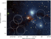 |
Fig. 1 Color-composite of the region in CrA we studied. The blue layer shows the Suprime-Cam/Subaru I band, and the green and red layers show J - and KS-band images from the VISIONS survey (Meingast et al. 2023) downloaded from the ESO science archive. The size of the field is 3 6.1 × 29.1 arcmin2. The small orange circles indicate members from Esplin & Luhman (2022), and the white stars denote objects observed with FLOYDS/LCO. The dotted white circles mark the fields in which targets for follow-up observations with KMOS/VLT were selected. |
2 Observations and data reduction
2.1 Imaging
Images in the I band (filter W-S-I+) taken with Suprime-Cam at the Subaru Telescope (Miyazaki et al. 2002) were downloaded from the Subaru archive. Suprime-Cam features ten 2048 × 4096 CCDs that cover a total field of view (FoV) of 34′ × 27′ with a pixel scale of 0.20″. The total on-source exposure time was 150 s, split into five individual exposures. We reduced the data with our own Python routines, including overscan subtraction, flat fielding, and correction for bad pixels and cosmic rays. The latter was performed using the package LACosmics (van Dokkum 2001). The five images for each detector were aligned using the package astroalign (Beroiz et al. 2020) and were combined using the median. The combined frames were coordinate-calibrated using Astrometry (Lang et al. 2010). The mean difference between the positions of the sources in our images and their respective values in Gaia Data Release 3 (DR3; Gaia Collaboration 2023) is 0.2″. Finally, a mosaic image was produced using the package reproject (Robitaille et al. 2020). The mosaic was only used for visualization purposes, but not for the further science analysis that was performed on the individual chip stacks to avoid differences in the background levels as a result of imperfect scaling between the chips and small-scale distortions observed at the edges of our stacks. The region we studied is shown in Fig. 1.
We identified and extracted the sources separately for each CCD using the software package Source-Extractor (Bertin & Arnouts 1996). To identify an object, we required at least 5 pixels to be above the 3σ threshold detection limit. We further rejected objects with Source-Extractor keywords FLAGS ≠ 0, and ELLIPTICITY ≥ 0.5.
We next retrieved J and KS photometry of the same region from the VISTA Hemisphere Survey (VHS; McMahon et al. 2013) and the I-band photometry from the Deep Near Infrared Survey of the Southern Sky (DENIS; Epchtein et al. 1999). The catalogs were cross-matched with a tolerance of 1″. The Suprime-Cam photometry was then calibrated using the following expression:
 (1)
(1)
where Iinstr is the Suprime-Cam instrumental magnitude, ZP is the zero point, and CT is the color term. Only stars with photometric errors ≤0.1 mag were taken into account for the calibration. The photometric uncertainties were calculated by combining the uncertainties of the zero point, color terms, and the measurement uncertainties supplied by Source-Extractor. At the end of the photometry calibration process, all catalogs from the different chips were joined into a single catalog. We averaged the sky positions and photometry for duplicate sources. To avoid effects of saturation in our catalog, we replaced the I-band photometry for sources brighter than I =16 mag by DENIS photometry. We also added brighter objects that were missing in our catalog, but were listed in DENIS and VHS. Our final catalog contains 19 599 sources. All the sources have I and J photometry, and 72% also contain a KS-band measurement.
In Fig. 2, we show the histograms for the three photometric bands and define the completeness limit as the magnitude at which the density of sources reaches a maximum value. We consider our catalog complete down to I ≈ 20.8 mag, J ≈ 19.5 mag, and KS ≈ 18.0 mag. According to BHAC15 models (Baraffe et al. 2015), the J - and KS -band limits corresponds to masses <0.01 M⊙ at the distance of 150 pc, age of 3 Myr, and the extinction of AV =0–5 mag; for the I band, this corresponds to masses from <0.01 and up to 0.015 M⊙.
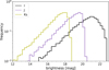 |
Fig. 2 Density of the sources in our catalog as a function of magnitude. |
2.2 Spectroscopic follow-up
In this section, we describe the observational setup and data reduction for the spectroscopic dataset. The details of the target selection for the spectroscopic follow-up are described in Section 3.
2.2.1 KMOS/VLT
The main part of the spectroscopic follow-up was performed between April and June 2023 using the K-band Multi Object Spectrograph (KMOS; Sharples et al. 2013) at the Very Large Telescope (VLT)1. KMOS performs integral field spectroscopy and has 24 arms, each with a square FoV of 2.8″ × 2.8″. The total FoV of the instrument is 7.2′ in diameter (dotted white circles in Fig. 1). KMOS was operated in service mode using a nod-to-sky ABA configuration, where A is the target and B is the sky. Between each exposure, a small dithering was performed. Eight different fields were observed with ten exposures of 133 s using the HK filter (~1.5-2.4 μm), providing a mean spectral resolving power of ~1800. The following calibrations were also obtained along with the target spectra: darks, flat field, arc lamp, and telluric standard stars.
The data were reduced using the KMOS pipeline (SPARK; Davies et al. 2013) in the ESO Reflex automated data reduction environment (Freudling et al. 2013). The pipeline produces calibrated 3D cubes by performing flat-field correction, wavelength calibration, sky subtraction, and telluric correction (using Molecfit; Smette et al. 2015). The spectra were extracted by fitting a 2D Gaussian to the reduced combined cube of each source. In total, 173 source spectra were extracted.
2.2.2 FLOYDS/LCO
In June and July 2021, we obtained optical spectra for eight objects using the Folded Low Order whYte-pupil Doubledispersed Spectrograph (FLOYDS) installed at the 2 m Faulkes South telescope, which is part of the Las Cumbres Observatory (LCO) robotic network2. The spectrograph provides a wide wavelength coverage of 3200–10 000 Å with a spectral resolution R~400-700, using the 1.6″ slit. We set an upper wavelength cutoff at 9000 Å as a result of the strong telluric absorption at longer wavelengths. In some cases, we also cut the bluest part of the spectrum when it presented a very low signal-to-noise ratio. The data reduction was identical to that described by Kubiak et al. (2021).
3 Search for low-mass members of CrA
3.1 Candidate selection
In Fig. 3 we show the I, I - J (left panel) and J, J - KS (right panel) color–magnitude diagrams (CMDs) of the studied region. The solid lines show various 3 Myr isochrones, consistent with the age of CrA. The red is from the BHAC15 model series (Baraffe et al. 2015), which extends only down to 0.01 M⊙. We also show somewhat older AMES-COND and AMES-DUSTY models (Allard et al. 2001), which were chosen because they extend into the planetary-mass regime. The latter models are available in the DENIS photometric system (important for our I-band photometry). We plot the prediction of the BHAC15 models using the Cousins I band, which should be fairly similar to the DENIS I band (≤0.05 mag difference; Delfosse 1997; Costa et al. 2006; Messineo 2022). This was further confirmed by cross-matching our catalog with that of Pancino et al. (2022), which yielded a mean difference of just 0.01 mag between our I-band magnitudes and their IC values, with a standard deviation of 0.03 mag.
The KMOS follow-up was designed to search for the lowest-mass BD and planetary population of the cluster. The objects for the follow-up were randomly selected from the purple shaded region shown in Fig. 3, which was constructed to extend the sequence of previously known members toward fainter magnitudes, taking the evolutionary models as a guide. We decided on the conservative blue-side limit guided by the AMES-COND model. The lower edge of the selection box corresponds to the spectroscopic sensitivity of KMOS (J=18 mag), and the upper edge was guided by the faint limit of Gaia DR3 (J ≈ 15 mag; I ≈ 17.8 mag). While the majority of the candidates fall below the Gaia sensitivity limit, a subset of the sources at the brighter end of the selection box do have Gaia astrometry. An overlap of about 1 mag with Gaia was allowed in order to ensure the completeness in the transition region. This selection box contains 404 objects, 173 of which were observed. No spectrum is available in the literature for any of the observed objects. The fields from which the objects were selected are marked by dotted white circles in Fig. 1. Their placement was chosen to maximize the number of targets that could be observed simultaneously.
The objects for the follow-up with the FLOYDS spectrograph were selected from the list of Gaia DR2 kinematic members (Galli et al. 2020a), except for object 5, which was chosen for its consistent proper motion and parallax from Gaia EDR3. This object and two more were later added to the census of CrA by Esplin & Luhman (2022) (see Appendix B).
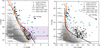 |
Fig. 3 CMDs showing the sources toward CrA (gray dots), along with the previously confirmed members (blue stars) from astrometry, spectroscopy, mid-infrared excess, or X-ray emission from Peterson et al. (2011), Galli et al. (2020a), and Esplin & Luhman (2022) The sources with spectroscopy obtained in this work are marked with black stars (FLOYDS) and circles (KMOS). The latter were selected from the purple shaded region. The completeness limit of our catalog is marked with the dashed black line, and the solid lines show the evolutionary models for the age of 3 Myr from the AMES-DUSTY (black), AMES-COND (orange), and BHAC15 (red) series (Allard et al. 2001; Baraffe et al. 2015). For clarity, masses are only marked on the AMES-COND model. The BHAC15 model extends to 0.01 M⊙. |
3.2 Spectral type and extinction
3.2.1 KMOS
Based on the candidate selection criteria described in the previous section, if they are confirmed as members of CrA, most of the KMOS/VLT candidates should have masses between ∼4 and 30 MJup. This implies an expected spectral type (SpT) later than ∼M7. These late-type sources can easily be recognized from their HK band spectra, and their youth can be assessed through the characteristic triangular shape of their H band caused by the effect of strong H2O absorption at both sides (Cushing et al. 2005; Allers & Liu 2013; Almendros-Abad et al. 2022).
We started our analysis by visual inspection and found that eight candidates show features resembling M dwarfs. The remaining objects mostly show flat or featureless spectra and are most probably background stars with a SpT earlier than M. They might also be galaxies. For the eight selected objects, we searched for the best-fit template spectrum using a χ2 minimization,
 (2)
(2)
where O is the object spectrum, T is the template spectrum, σ is the noise of the observed spectrum, N is the number of data points, and m is the number of fitted parameters (m=2). The latter are the SpT and extinction, which can be fit simultaneously. In the fitting process, we used young and field spectral templates. The young templates were taken from Luhman et al. (2017) and are defined at half-integer SpTs from M0 to L0, complemented with L2, L4, and L7. The field templates, defined in the range M0–L9 at each 1 subclass interval, were taken from Kirkpatrick et al. (2010). Each object was compared with all the spectral templates for a wide range of extinction values: AV=0–20 mag with a step of 0.5 mag. We used the extinction law from Wang & Chen (2019), which assumes RV=3.1. The object spectra were resampled to match the wavelength grid of the templates. The comparison was made for the H and K bands, neglecting the telluric region in between 1.8 and 1.95 µm. All the spectra were normalized at 1.65 µm.
The fits confirmed that the eight candidates have SpT M, the latest type is M6. In all cases, the field templates provide a better fit. Additionally, we calculated the T LI - g gravity-sensitive spectral index (Almendros-Abad et al. 2022) and found that seven objects are compatible with field dwarfs. The spectrum quality of the remaining object is poor, and with I = 21.4 mag and J = 17.6 mag, it is too faint to be a young mid-M dwarf in the cluster. In conclusion, none of the candidates observed with KMOS is found to be a very low-mass member of the CrA SFR. In Appendix A, we show a selection of the KMOS spectra and provide coordinates of all the objects that were included in the KMOS follow-up.
We note that proper motion and parallax data are available from Gaia DR3 for 27 of the objects observed with KMOS. None of them is consistent with membership in CrA. As mentioned before, some overlap with Gaia was intentional when we defined the selection box for the spectroscopic follow-up. We recognize that with Gaia DR3 available at the time of planning the observations, a more refined selection excluding known kinematic nonmembers would have improved the efficiency of the KMOS spectroscopic campaign, however.
Objects that were followed up on using FLOYDS.
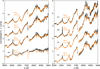 |
Fig. 4 Spectra of the eight members observed with FLOYDS/LCO (black), along with the best-fit reddened template spectra (orange). All the spectra were normalized at 7400 Å. The Hα emission in the template spectra was masked for clarity. |
3.2.2 FLOYDS
The follow-up with FLOYDS was executed before the publication of the study by Esplin & Luhman (2022), in which all of the eight objects appear as kinematic members, and they were additionally confirmed by spectroscopy. Spectra for several objects are also available in earlier studies (Walter et al. 1997; Romero et al. 2012; Sicilia-Aguilar et al. 2008, 2011). We derived the SpTs and extinction using the χ2 minimization (Eq. (2)) and used spectra of young objects (1–10 Myr) from Luhman et al. (2003), Luhman (2004a,b,c), Bayo et al. (2011), and Venuti et al. (2019) as templates. Their SpTs are M0.5–M9 with a step of 0.25–0.5 spectral subtypes. The best-fit results are given in Table 1 and shown in Fig. 4. The derived SpTs agree very well with those found in the literature.
4 Substellar census and the IMF in CrA
4.1 Estimate of the number of missing CrA members
Using the statistics gained from the spectroscopic survey, we estimated the number of members that are missing in the current census of CrA. Similar to the works from the SONYC series, we used the confirmation rates of our spectroscopic follow-up to estimate the expected number of members among the remaining photometric candidates. We defined the confirmation rate as the number of confirmed members divided by the number of candidates with spectroscopy. The uncertainties are represented as 95% confidence intervals, calculated using the Clopper–Pearson method (suitable for small-number events; Gehrels 1986; Brown et al. 2001).
We assumed that the census of CrA members is largely complete for sources above our selection area in Fig. 3 (I < 17.8 mag). The vast majority of objects at these magnitudes have astrometric data from Gaia, which were effectively used to identify candidate members (Galli et al. 2020a; Esplin & Luhman 2022). The extent of the Gaia coverage in this region of the CMD is also evident in Fig. B.1.
To estimate the number of potential members that are still missing in our census, we focused on objects that fall within the selection area (purple-shaded region) and are brighter than the completeness limit (dashed line in Fig. 3). The known members (blue stars in the same figure) were excluded from the analysis. The total number of objects was then 153, of which we took 77 spectra. The confirmation rate is therefore 0/77 = 0 , which means that the 78 objects without spectra are expected to contain 0 to 4 members that are undetected so far. When we repeated the same analysis without the objects rejected by Gaia data (Galli et al. 2020a), the selection box contained 78 objects, 57 of which were observed with KMOS. This yields a confirmation rate of
  , and 0 to 1 missing objects. Furthermore, we restricted our selection to objects lying to the right of the AMES-DUSTY isochrone. Originally, our selection was guided by the AMES-COND model, which may be too blue at substel-lar masses (judging from the sequence of known members). We therefore repeated the same analysis as before and only kept the sources to the right of the AMES-DUSTY model. This resulted in 0–5 missing objects without the Gaia rejections, and 0–3 missing objects with these rejections.
In summary, our analysis shows that the current census in CrA may be missing five objects at most, with masses between 0.006 and 0.07 M⊙(estimated in Section 4.2).
4.2 Derivation of mass and extinction
The masses were derived for the known members that were contained in the latest census by Esplin & Luhman (2022) and for the objects in our selection box that were not followed-up spectroscopically. For the latter, these mass estimates are conditional on the assumption that the object is a true member of CrA, which we know may only hold for a small subset of these objects (Section 4.1). These mass estimates were used to correct the IMF for the objects that might be missing in the census.
To estimate the mass and the extinction of an object, we de-reddened its photometry to the 3 Myr isochrone in the I, I - J CMD, which was shifted to the distance of the cluster given in Galli et al. (2020a). The uncertainty on the distance is small (< 1 pc) and has no effect on the mass estimate. We used the extinction law from Wang & Chen (2019). The procedure described here was repeated for each of the three isochrones shown in Fig. 3. The choice of the age was driven by the range of age estimates of CrA in the literature, which varies between 1 and 5 Myr (Neuhäuser & Forbrich 2008; Galli et al. 2020a; Esplin & Luhman 2022). At the same time, the disk fraction was estimated to be around 50% (López Martí et al. 2010; Peterson et al. 2011; Esplin & Luhman 2022), which is consistent with an age of 2–3 Myr (Stolte et al. 2015; Richert et al. 2018; Michel et al. 2021; Winter & Haworth 2022).
To assess how photometric uncertainties affect the determination of extinction and mass, we employed a Monte Carlo approach. For each source, we generated 1000 synthetic magnitudes per band, drawing from a normal distribution centered on the observed value, with a standard deviation equal to the corresponding photometric uncertainty. For each of these 1000 realizations, we then derived the mass and extinction by dereddening the photometry to match the isochrone. The final AV value for each source was taken as the average across all realizations, with its uncertainty given by the standard deviation. The resulting mass distributions were typically not normally distributed, however, because magnitude and mass are not linearly related. To account for this, we retained the full distributions of mass for each source. These were then used to draw individual mass values during the Monte Carlo simulation we used to derive the IMF and star-to-BD number ratio.
4.3 Initial mass function in CrA
To derive the IMF, we took all the previously confirmed members of CrA located within our survey region from the latest census of Esplin & Luhman (2022). We complemented this with the results of our spectroscopic survey, which give a stringent upper limit on the number of members that might be missing within our selection box. The stellar masses were sampled from the mass distributions derived in Section 4.2. This sampling was repeated 100 times for each source, resulting in 100 cluster mass distributions. For each of these 100 realizations, we performed 100 bootstrap re-samplings, that is, random selections with replacement. Each bootstrap involved drawing a new sample of N stars (where N is the size of the realization) with replacement, allowing individual stars to be selected multiple times or not at all. This procedure yielded a total of 10 000 mass distributions, which were then used to compute the mass function along with the associated uncertainties. The IMFs are plotted using a variable size with the aim to maintain a roughly constant number of objects in each bin.
To account for objects that might be missing in the census, we repeated the IMF derivation and randomly selected five objects without spectra from our selection box. We repeated the process 100 times to ensure the statistical robustness of the result. As estimated in Section 4.1, this is an upper limit on the number of missing objects. The resulting IMFs, in power-law and lognormal forms, are shown in Fig. 5 for three different evolutionary models. The black symbols and the gray histogram represent the IMF after correcting for the missing objects, which affects only the two lowest-mass bins. The orange points indicate the IMF before this correction. For reference, the dotted and dashed lines show the IMFs from Kroupa (2001) and Chabrier (2005), respectively. While our overall results are consistent with the former, we note discrepancies with the latter. Specifically, our IMF does not exhibit the sharp decline in the number of substellar objects predicted by the Chabrier functional form. A similar behavior was also observed in earlier works (e.g., Peña Ramírez et al. 2012; Mužic´ et al. 2019; Miret-Roig et al. 2022).
To enable comparison with previous works, we fit a powerlaw function to the IMFs shown in the top panels for three different mass ranges. First, we fit a single slope over the entire available mass range (0.01–1 M⊙). We also provide slopes over the mass range 0.01–0.2 M⊙, and finally, in the substellar regime (0.01–0.1 M⊙). By comparing the slope across these different mass ranges, we observe a gradual flattening of the IMF. The flattening is less pronounced in the case of the BHAC15 model, which may be partially attributed to the fact that this model does not extend below 0.01 M⊙. As a result, the mass distributions for objects near this limit are truncated at the low-mass end. The fitting was carried out for the original IMF and for the version that included additional (missing) objects. As the true distribution likely lies between these two cases, we report in Table 2 the average value of the slope α. For the full mass range (0.01–1 M⊙), we obtain α = 0.95 ± 0.06. In the range 0.01–0.2 M⊙, the slope is α = 0.63 ± 0.14, and in the substellar range (0.01–0.1 M⊙), α = 0.33 ± 0.19.
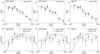 |
Fig. 5 IMF in CrA in the power-law (top panels) and the log-normal form (bottom panels). The masses were derived using three different 3 Myr evolutionary models, indicated in the upper left corner of each panel. The black symbols and the gray histogram represent the IMF after correcting for the missing objects, and the orange points indicate the two affected bins before this correction. The orange points were slightly shifted to the left of the black points for clarity; the bin centers and sizes were maintained. Two different IMF representations are shown: dN/dm (top panels) and dN/dlog(m) (bottom panels). The dotted line shows the Kroupa segmented power-law mass function (Kroupa 2001), and the dashed line shows the Chabrier mass function (Chabrier 2005), both normalized to match the total number of objects in the cluster. |
4.4 Star-to-brown dwarf ratio
To estimate the ratio of the number of stars and that of BDs, we used the mass estimates derived in Section 4.2 and applied the same Monte Carlo method we used to derive the IMF. We generated 10 000 mass distributions. The boundary between stellar and substellar objects is defined at 0.075 M⊙, corresponding to the hydrogen-burning limit at solar metallicity. We computed the ratio using two lower-mass limits on the BD side: 0.02 M⊙and 0.03 M⊙. For the stellar population, we adopted an upper mass limit of 1 M⊙, as is commonly done in the literature. The resulting distributions of the star-to-BD ratio are shown in Fig. 6 and are also summarized in Table 2 for each of the three isochrones we considered. The quoted values represent the median of each distribution, and the uncertainties refer to the 95% confidence limits. We note that the star-to-BD ratio is only minimally affected by the missing sources. We therefore only report results for the uncorrected case. The star-to-BD ratio in CrA is ∼2, but with a relatively wide plausible range, which is mainly the consequence of the small number of members combined with the uncertainties in mass determination.
Slope α of the IMF in CrA in the power-law form and star-to-BD number ratio for three different sets of isochrones.
5 Comparison to other regions
In this section, we compare the IMF and star-to-BD ratio derived for CrA with those from our previous works, which includes three nearby SFRs studies in the SONYC series3 (Cha I, Lupus 3, and NGC 1333; Scholz et al. 2012b; Mužic´ et al. 2015), and the two massive clusters RCW 38 and NGC 2244 taken from Mužic´ et al. (2017, 2019)4.
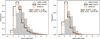 |
Fig. 6 Distribution of the star-to-BD ratio obtained from our data for three different isochrones. The mass ranges used to calculate the ratio are indicated in each panel. The correction for potentially missing objects in the CrA census was not applied because their inclusion has little effect on the determination of the star-to-BD ratio. |
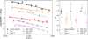 |
Fig. 7 Left: comparison of the IMFs below 1 M⊙ in six different SFRs. The IMF for CrA is the mean of the IMFs presented in Section 4.3. The solid lines represent fits to the full set of data points for each cluster, and the dashed lines indicate fits restricted to the substellar regime below 0.2 M⊙. Right: IMF slope α corresponding to the fits displayed in the left panel, indicated using matching line styles. Table 3 lists the values shown in this panel, along with the references. |
5.1 IMF comparison
In Fig. 7, we present the IMFs of CrA and the other five regions listed above. For the full mass range below 1 M⊙, the values of α range between 0.6 and 1 (see Table 3). The IMF in CrA is on the steeper side of this range, similar to NGC 2244 and Lupus 3 (α ∼ 1). A similarly steep slope (α = 1 ± 0.2) has also been derived for Berkeley 59 over the mass range 0.04–0.4 M⊙(Panwar et al. 2024). Several IMFs shown in Fig. 7 show some degree of flattening in the substellar regime. To illustrate this, we also show the fit to the IMF below 0.2 M⊙(dashed lines). The flattening is most significant in RCW 38 (see right panel of Fig. 7) and Lupus 3, but because of the small number of points in the IMF, the error bar on the latter result is also quite large. For CrA, the flattening becomes more clearly pronounced at masses below 0.1 M⊙, as discussed in Section 4.3.
Flat slopes in the substellar regime have been reported in σ Ori (α = 0.2 ± 0.2) for the masses 0.004–0.19 M⊙(Damian et al. 2023). Earlier studies of the same cluster reported a slope of ∼0.6 for a similar mass range (Caballero et al. 2007; Peña Ramírez et al. 2012). Damian et al. (2023) likely provided a more reliable representation of the cluster based on a complete sample of spectroscopically confirmed members. In 25 Ori, Suárez et al. (2019) reported a slope α = 0.26 ± 0.04 for the masses between 0.012 and 0.4M⊙. With the exception of Lupus 3, all other regions shown in Fig. 7 show an IMF slope α ≳ 0.5 for the masses below 0.2M⊙. If taken at face value, the scatter in the slope α may appear to be significant, but it is important to emphasize that the error bars given in Table 3 and in most other works only reflect statistical uncertainties and do not account for other potential sources of error or systematics, such as uncertainties in distance and age, the choice of isochrones, or the adopted extinction law.
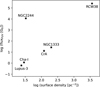 |
Fig. 8 Stellar surface density vs. the median FUV flux for the six SFRs and clusters discussed in the text. |
5.2 Comparison of the star-to-BD ratios
To facilitate a comparison of the star-to-BD number ratios, we include the corresponding values in Table 3 for the same set of regions used in the IMF analysis. The star-to-BD ratios span a range of approximately 2–5. As discussed by Scholz et al. (2013), this range reflects various sources of uncertainty in the mass determination, issues related to the membership, and the small sample sizes. It is worth noting that the regions listed in Table 3 represent different star-forming environments, which we attempted to characterize using their average stellar density and incident far-ultraviolet (FUV) flux (see Fig. 8)5. The environment of CrA is most similar to that of NGC 1333 because both regions are denser and have stronger FUV radiation fields than the other nearby SFRs Lupus 3 and Cha I. The two massive clusters NGC 2244 and RCW 38 also occupy distinct positions in this parameter space, both characterized by very strong radiation fields, but representing opposite extremes in terms of stellar density.
Figure 9 shows the star-to-BD ratio for the six regions discussed in this section, plotted as a function of stellar surface density. Each region is represented by a rectangle of arbitrary width, with its color indicating the median FUV flux within the region. Fig. 10 shows a similar plot for the values of the IMF slope α for the fits over two different mass ranges (given in Table 3. At this point, neither the IMF nor the star-to-BD ratio shows a significant dependence on the cluster stellar density or the ionizing flux from the most massive stars. A combined effect, where one property might promote BD formation while the other suppresses it, also appears unlikely because the sample includes regions that span a range of both parameters. For instance, ChaI has fewer BDs per star than NGC 2244, and the main difference between the two clusters is their FUV radiation levels. Conversely, NGC 2244 and NGC 1333 exhibit similar star-to-BD ratios although the FUV flux in NGC 2244 is higher by three orders of magnitude. RCW38 also shows a comparable ratio, even though its stellar density is far higher than that of the two clusters.
Recently, Gupta et al. (2024) compiled literature values for the star-to-BD ratio for 15 young clusters and SFRs. They reported that the ratio decreases with stellar density, but shows no clear correlation with the incident UV flux. Based on our analysis, we do not observe a similar decrease in the star-to-BD ratio with stellar density. First of all, as noted in their paper, the star-to-BD ratios for some clusters were derived by extrapolating the stellar IMF into the substellar regime. This included Wester-lund 1, which has the lowest ratio in their sample of 15 clusters. It therefore significantly influences the claim of environmental dependence. Additionally, several of the SONYC-derived values were presented with error bars that appear underestimated relative to those in the original publications. For these reasons, we approach the results of Gupta et al. (2024) with caution. Although our sample is more controlled, it remains limited in size. Furthermore, our analysis of NGC 2244 and RCW 38 is confined to the central regions of the two clusters. Additional observational efforts are essential to reliably evaluate the impact of stellar density on BD formation, especially in more extreme environments. In parallel, a more uniform treatment of existing datasets would help us to mitigate various sources of systematic uncertainty. For this reason, we mainly focus our comparisons on clusters that we studied within our own work, although even this approach presents challenges because the nature of the field evolves, such as updates to distances, extinction laws, and theoretical models over the extended period during which the data were collected.
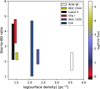 |
Fig. 9 Star-to-BD ratio in various SFRs as a function of stellar surface density. Each rectangle represents a different cluster, and the height corresponds to the range of star-to-BD ratios; the width was chosen arbitrarily. The color of each rectangle indicates the median FUV flux in the region. |
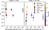 |
Fig. 10 IMF slope α as a function of stellar surface density, fit for the masses <1 M⊙ (left) and <0.2 M⊙ (right). The points are colored by the median FUV flux of each region, similar to Fig. 9. |
6 Summary and conclusions
We conducted a comprehensive survey of the substellar population in the CrA SFR in order to derive its IMF and characterize its low-mass stellar and substellar content. Our approach combined deep optical imaging from Suprime-Cam/Subaru, nearinfrared data from the VHS, and follow-up spectroscopy with KMOS/VLT and FLOYDS/LCO.
The optical spectroscopy of eight kinematically selected candidates using FLOYDS/LCO confirmed them as low-mass stellar members with SpTs M1 to M5. In contrast, from a photometric sample of 173 BD candidates identified based on CMDs and evolutionary models, none was confirmed as a substellar member of CrA. The KMOS spectroscopic analysis revealed that these objects are predominantly field contaminants, with spectra inconsistent with young late-type substellar sources. Nevertheless, these objects helped us to make stringent constraints on the number of low-mass members that might be missing in the census. Combining our results with the latest census by Esplin & Luhman (2022), we estimate that five substellar objects may still be missing from the CrA population at most.
We derived the CrA IMF over the mass range 0.01–1 M⊙and found a power-law slope of α = 0.95 ± 0.06. In the range 0.01– 0.02M⊙, the slope is α = 0.63 ± 0.14, and in the substellar range (0.01–0.1 M⊙), it is α = 0.33 ± 0.19, indicating the flattening of the IMF in the substellar regime. The star-to-BD number ratio in CrA is ∼2. For consistent comparisons, we re-derived the IMFs and star-to-BD ratios for Cha I and Lupus 3 from the SONYC survey and incorporated updated Gaia distances and consistent evolutionary models. For Cha I, we derive α = 0.62 ± 0.13 over the mass range 0.01–1 M⊙, with a star-to-BD ratio of ∼3.2–4.8. For Lupus 3, we find α = 0.98 ± 0.38 for the mass range 0.02– 1 M⊙, with a star-to-BD ratio of ∼2.1–4.5.
Finally, we examined the relation between the star-to-BD ratio and environmental factors, including the stellar surface density and median FUV flux, which were both consistently derived for the six comparison regions. The stellar surface density varies by over two orders of magnitude, while the FUV fluxes span approximately five orders of magnitude. Our results show no significant correlation between these properties and the relative abundance of BDs. This suggests that environmental conditions such as stellar density and ionizing radiation from massive stars do not strongly affect the formation of BDs. Our results do not confirm earlier claims of a dependence on the stellar surface density (Gupta et al. 2024) and instead support the idea of a largely universal substellar IMF across a range of starforming environments, at least within the limits of the current uncertainties.
Data availability
Full Table A.1 is available at the CDS via https://cdsarc.cds.unistra.fr/viz-bin/cat/J/A+A/701/A147.
Acknowledgements
KM and AdB-dV acknowledges support from the Fundação para a Ciência e a Tecnologia (FCT) through the CEEC-individual contract 2022.03809.CEECIND (DOI 10.54499/2022.03809.CEECIND/CP1722/CT0001), and the project 2023.01915.BD (DOI 10.54499/2023.01915.BD). KM also acknowledges support from the Scientific Visitor Programme of the European Southern Observatory (ESO) in Chile. BD and AS acknowledge support from the UKRI Science and Technology Facilities Council through grant ST/Y001419/1/. VA-A acknowledges support from the INAF grant 1.05.12.05.03.
Appendix A KMOS spectra
Table A.1 provides the coordinates of all objects included in the KMOS follow-up observations. The first eight entries correspond to sources consistent with field M dwarfs (see Section 3.2.1), while the remaining spectra are inconclusive, i.e., they have been ruled out as young M-type dwarf stars or BDs. In Figure A.1, we show a subset of the KMOS spectra.
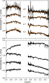 |
Fig. A.1 Subset of the KMOS spectra. Top: Several confirmed field M dwarfs (in black), overlaid with their corresponding best-fit field dwarf templates (in orange). Object IDs are indicated and correspond to those listed in Table A.1. Bottom: Selection of other spectra from our sample, which can be clearly excluded as young, low-mass M-type stars or BDs. |
Objects included in the KMOS follow-up (extract).
Appendix B Objects rejected in Galli et al. (2020a)
In Fig. B.1 we show a portion of the CMD shown in Fig. 3, where exists an overlap between the objects with kinematics from Gaia DR2 studied in Galli et al. (2020a) and our spectroscopic followup with KMOS. The symbols are identical to those in Fig. 3, with an addition of kinematically rejected sources from Galli et al. (2020a), which are shown as orange points. Three sources originally rejected in this work, were later confirmed as members in Esplin & Luhman (2022).
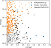 |
Fig. B.1 Zoom into the CMD region with an overlap of the KMOS follow-up with Gaia data. The sources in our catalog are shown as grey dots, previously confirmed members from astrometry, spectroscopy, mid-infrared excess, or X-ray emission as blue stars (Peterson et al. 2011; Galli et al. 2020a; Esplin & Luhman 2022), and objects rejected in (Galli et al. 2020a) as orange crosses. The sources with spectroscopy with KMOS are marked with black circles. |
Appendix C Updates of SONYC IMFs in Cha I and Lupus 3
In Mužic´ et al. (2015), we published the IMFs in Cha I and Lupus 3 SFRs, assuming the distances of 160 pc and 200 pc, respectively. In the meantime, these distances have been updated thanks to Gaia, to 190 pc for Cha I (Galli et al. 2021), and 160 pc to Lupus 3 (Galli et al. 2020b). Given the significant discrepancy with the old distances, we recalculated the two IMFs and the corresponding star-to-BD ratios, repeating the identical procedure from the original paper. The newly obtained slopes are consistent with the old ones within the uncertainties. For Cha I, the IMF slope in the range 0.01–1 M⊙ changed from 0.78 ± 0.08 to 0.62 ± 0.13, and for Lupus 3 the slope changed from 0.79 ± 0.13 to 0.98 ± 0.38, for the mass range 0.02–1 M⊙. We note also that the distance to NGC 1333 used in SONYC (Scholz et al. 2012b) is similar to the new distance based on Gaia (Ortiz-León et al. 2018), requiring no update.
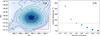 |
Fig. C.1 Spatial distribution of members in CrA is shown in the left panel (black dots), overlaid with a two-dimensional kernel density estimate (color map). Contours indicate regions enclosing different percentages of the sources. The corresponding stellar surface densities within each contour are presented in the right panel, with the horizontal dashed line marking the surface density at the 50% contour level. The red bar in the lower right corner of the left panel represents a scale of 0.5 pc at the distance of CrA. |
Appendix D Stellar surface densities
We estimate the surface density of the CrA on-cloud population following the same approach used for other regions in Mužic´ et al. (2019). Specifically, we apply a two-dimensional kernel density estimation with a Gaussian kernel to the spatial distribution of cluster members, considering only sources with SpTs earlier than M7. From the resulting kernel density estimation map, we define density contours enclosing fixed percentages of members, ranging from 20% to 90% (see Fig.C.1). For each contour, we compute the stellar surface density, as shown in the right panel of Fig. C.1. Consistent with Mužic´ et al. (2019) and Almendros-Abad et al. (2023), we adopt the surface density corresponding to the 50% contour level as a reference value for comparison across regions. For CrA, this value is 120 stars per pc2.
We also calculated the new values for the stellar surface densities in Cha I and Lupus 3, using the updated distances (see Appendix C). The values are listed in Table 3.
Appendix E Estimate of the FUV flux
Massive stars in a cluster produce a background UV field, which can provide feedback on the star and BD formation process. The amount of radiation cluster stars receive depends on the luminosity of the most massive stars and their distance to other stars. To estimate the FUV field of each cluster, we start by compiling a list of its O and B stars; relevant details and the references are listed at the end of this section. For each spectral subtype, we assume the effective temperature and luminosity from Pecaut & Mamajek (2013). The FUV flux is often expressed in terms of the Habing unit G0=1.6 × 10⁻³ erg s−1 cm−2, the amount of radiation found for the solar neighbourhood in the wavelength range between 912Å and 2400Å (Habing 1968). To estimate a star’s FUV luminosity, we scale its total luminosity by the factor calculated using Eq. 4 of Kunitomo et al. (2021), specifying the fraction of light emitted in the FUV at a given temperature. The flux received by each cluster star is calculated by dividing the luminosity of each OB source by the square of its distance from the star. Since we only have access to the projected distances in two dimensions, we assume that the distance along the line of sight is half of the projected separation in the plane of the sky. For each cluster member, we sum the contributions from all ionizing sources. As a measure of the FUV field strength within the cluster, we adopt the median of the fluxes received by all individual stars.
The locations and SpTs of OB stars come from the following sources.
CrA: Four B8-9 stars in the on-cloud population from Esplin & Luhman (2022);
Cha I: One B6 and two B9/A0 stars from Luhman (2007) and Kirk & Myers (2011);
Lupus 3: One B4 member from Kirk & Myers (2011);
NGC 1333: Two B-type stars (B5 and B8) from Luhman et al. (2016);
NGC 2244: Seven O4-O9 and 24 B-type stars from Martins et al. (2012) and Wang et al. (2008);
RCW 38: One O5.5 binary (IRS 2; DeRose et al. 2009 and 17 B-type candidates located in the central part of the cluster from Wolk et al. (2008). For these candidates, we assign SpTs according to their bolometric luminosities from Wolk et al. (2008) following the stellar properties as listed in Pecaut & Mamajek (2013).
Recently, Anania et al. (2025) computed the FUV fluxes for stars bearing discs in 15 regions within ~500 pc. Fundamentally, their method is similar to ours in that it considers the FUV luminosities of OBA stars and estimates their combined influence on individual stars. The primary difference lies in how they estimate the 3D separations between disc-bearing stars and the massive sources. For CrA, they report a median FUV flux of FFUV, median =  , consistent with our estimate. However, for Cha I, our value of 1.2 is lower than the
  reported by Anania et al. (2025). In contrast, our Cha I estimate aligns with the value reported in Gupta et al. (2024), but for three other regions (NGC 1333, NGC 2244, and RCW 38), their estimates appear systematically higher than ours. It is unclear at which distance the fluxes in Gupta et al. (2024) were calculated, as they only describe how the FUV luminosities were derived.
Given the challenges involved in estimating the FUV fluxes experienced by cluster members, it is perhaps unsurprising that the absolute values reported in different studies show some discrepancies. However, when considered in relative terms, there is broad agreement. For instance, Chamaeleon and Lupus are consistently identified as regions with the lowest median FUV flux, while RCW 38 stands out with fluxes orders of magnitude higher, closely followed by NGC 2244. NGC 1333, in contrast, occupies an intermediate position between these extremes.
References
- Allard, F., Hauschildt, P. H., Alexander, D. R., Tamanai, A., & Schweitzer, A. 2001, ApJ, 556, 357 [Google Scholar]
- Allers, K. N., & Liu, M. C. 2013, ApJ, 772, 79 [NASA ADS] [CrossRef] [Google Scholar]
- Almendros-Abad, V., Mužic´, K., Moitinho, A., Krone-Martins, A., & Kubiak, K. 2022, A&A, 657, A129 [NASA ADS] [CrossRef] [EDP Sciences] [Google Scholar]
- Almendros-Abad, V., Mužic´, K., Bouy, H., et al. 2023, A&A, 677, A26 [NASA ADS] [CrossRef] [EDP Sciences] [Google Scholar]
- Alves de Oliveira, C., Moraux, E., Bouvier, J., & Bouy, H. 2012, A&A, 539, A151 [NASA ADS] [CrossRef] [EDP Sciences] [Google Scholar]
- Anania, R., Winter, A. J., Rosotti, G., et al. 2025, A&A, 695, A74 [NASA ADS] [CrossRef] [EDP Sciences] [Google Scholar]
- Baraffe, I., Homeier, D., Allard, F., & Chabrier, G. 2015, A&A, 577, A42 [NASA ADS] [CrossRef] [EDP Sciences] [Google Scholar]
- Bayo, A., Barrado, D., Stauffer, J., et al. 2011, A&A, 536, A63 [NASA ADS] [CrossRef] [EDP Sciences] [Google Scholar]
- Beroiz, M., Cabral, J. B., & Sanchez, B. 2020, Astron. Comput., 32, 100384 [NASA ADS] [CrossRef] [Google Scholar]
- Bertin, E., & Arnouts, S. 1996, A&AS, 117, 393 [NASA ADS] [CrossRef] [EDP Sciences] [Google Scholar]
- Boley, A. C., Payne, M. J., & Ford, E. B. 2012, ApJ, 754, 57 [Google Scholar]
- Bouy, H., Tamura, M., Barrado, D., et al. 2022, A&A, 664, A111 [NASA ADS] [CrossRef] [EDP Sciences] [Google Scholar]
- Brown, L. D., Cai, T. T., & Dasgupta, A. 2001, Statist. Sci., 16, 101 [Google Scholar]
- Caballero, J. A., Béjar, V. J. S., Rebolo, R., et al. 2007, A&A, 470, 903 [NASA ADS] [CrossRef] [EDP Sciences] [Google Scholar]
- Chabrier, G. 2005, in Astrophysics and Space Science Library, 327, The Initial Mass Function 50 Years Later, eds. E. Corbelli, F. Palla, & H. Zinnecker, Astrophysics and Space Science Library, 327, 41 [Google Scholar]
- Costa, E., Méndez, R. A., Jao, W. C., et al. 2006, AJ, 132, 1234 [CrossRef] [Google Scholar]
- Cushing, M. C., Rayner, J. T., & Vacca, W. D. 2005, ApJ, 623, 1115 [Google Scholar]
- Daffern-Powell, E. C., Parker, R. J., & Quanz, S. P. 2022, MNRAS, 514, 920 [Google Scholar]
- Damian, B., Jose, J., Samal, M. R., et al. 2021, MNRAS, 504, 2557 [NASA ADS] [CrossRef] [Google Scholar]
- Damian, B., Jose, J., Biller, B., et al. 2023, ApJ, 951, 139 [NASA ADS] [CrossRef] [Google Scholar]
- Davies, R. I., Agudo Berbel, A., Wiezorrek, E., et al. 2013, A&A, 558, A56 [NASA ADS] [CrossRef] [EDP Sciences] [Google Scholar]
- Delfosse, X. 1997, Theses, Universite Scientifique et Medicale de Grenoble, Grenoble, France [Google Scholar]
- DeRose, K. L., Bourke, T. L., Gutermuth, R. A., et al. 2009, AJ, 138, 33 [CrossRef] [Google Scholar]
- Dzib, S. A., Loinard, L., Ortiz-León, G. N., Rodríguez, L. F., & Galli, P. A. B. 2018, ApJ, 867, 151 [Google Scholar]
- Epchtein, N., Deul, E., Derriere, S., et al. 1999, A&A, 349, 236 [NASA ADS] [Google Scholar]
- Esplin, T. L., & Luhman, K. L. 2022, AJ, 163, 64 [NASA ADS] [CrossRef] [Google Scholar]
- Freudling, W., Romaniello, M., Bramich, D. M., et al. 2013, A&A, 559, A96 [NASA ADS] [CrossRef] [EDP Sciences] [Google Scholar]
- Gaia Collaboration, (Vallenari, A., et al.) 2023, A&A, 674, A1 [NASA ADS] [CrossRef] [EDP Sciences] [Google Scholar]
- Galli, P. A. B., Bouy, H., Olivares, J., et al. 2020a, A&A, 634, A98 [NASA ADS] [CrossRef] [EDP Sciences] [Google Scholar]
- Galli, P. A. B., Bouy, H., Olivares, J., et al. 2020b, A&A, 643, A148 [EDP Sciences] [Google Scholar]
- Galli, P. A. B., Bouy, H., Olivares, J., et al. 2021, A&A, 646, A46 [NASA ADS] [CrossRef] [EDP Sciences] [Google Scholar]
- Gehrels, N. 1986, ApJ, 303, 336 [Google Scholar]
- Gupta, S., Jose, J., Das, S. R., et al. 2024, MNRAS, 528, 5633 [Google Scholar]
- Habing, H. J. 1968, Bull. Astron. Inst. Netherlands, 19, 421 [Google Scholar]
- Haworth, T. J., Facchini, S., & Clarke, C. J. 2015, MNRAS, 446, 1098 [NASA ADS] [CrossRef] [Google Scholar]
- Hennebelle, P., & Grudic´, M. Y. 2024, ARA&A, 62, 63 [Google Scholar]
- Kirk, H., & Myers, P. C. 2011, ApJ, 727, 64 [Google Scholar]
- Kirkpatrick, J. D., Looper, D. L., Burgasser, A. J., et al. 2010, ApJS, 190, 100 [Google Scholar]
- Kirkpatrick, J. D., Marocco, F., Gelino, C. R., et al. 2024, ApJS, 271, 55 [NASA ADS] [CrossRef] [Google Scholar]
- Kroupa, P. 2001, MNRAS, 322, 231 [NASA ADS] [CrossRef] [Google Scholar]
- Kubiak, K., Mužic´, K., Sousa, I., et al. 2021, A&A, 650, A48 [NASA ADS] [CrossRef] [EDP Sciences] [Google Scholar]
- Kunitomo, M., Ida, S., Takeuchi, T., et al. 2021, ApJ, 909, 109 [NASA ADS] [CrossRef] [Google Scholar]
- Lang, D., Hogg, D. W., Mierle, K., Blanton, M., & Roweis, S. 2010, AJ, 139, 1782 [Google Scholar]
- Langeveld, A. B., Scholz, A., Mužic´, K., et al. 2024, AJ, 168, 179 [Google Scholar]
- Lodieu, N., Zapatero Osorio, M. R., Béjar, V. J. S., & Peña Ramírez, K. 2018, MNRAS, 473, 2020 [Google Scholar]
- López Martí, B., Spezzi, L., Merín, B., et al. 2010, A&A, 515, A31 [NASA ADS] [CrossRef] [EDP Sciences] [Google Scholar]
- Luhman, K. L. 2004a, ApJ, 602, 816 [NASA ADS] [CrossRef] [Google Scholar]
- Luhman, K. L. 2004b, ApJ, 616, 1033 [Google Scholar]
- Luhman, K. L. 2004c, ApJ, 617, 1216 [Google Scholar]
- Luhman, K. L. 2007, ApJS, 173, 104 [Google Scholar]
- Luhman, K. L. 2012, ARA&A, 50, 65 [CrossRef] [Google Scholar]
- Luhman, K. L., Briceño, C., Stauffer, J. R., et al. 2003, ApJ, 590, 348 [Google Scholar]
- Luhman, K. L., Esplin, T. L., & Loutrel, N. P. 2016, ApJ, 827, 52 [Google Scholar]
- Luhman, K. L., Mamajek, E. E., Shukla, S. J., & Loutrel, N. P. 2017, AJ, 153, 46 [Google Scholar]
- Martins, F., Mahy, L., Hillier, D. J., & Rauw, G. 2012, A&A, 538, A39 [NASA ADS] [CrossRef] [EDP Sciences] [Google Scholar]
- McMahon, R. G., Banerji, M., Gonzalez, E., et al. 2013, The Messenger, 154, 35 [NASA ADS] [Google Scholar]
- Meingast, S., Alves, J., Bouy, H., et al. 2023, A&A, 673, A58 [NASA ADS] [CrossRef] [EDP Sciences] [Google Scholar]
- Messineo, M. 2022, PASJ, 74, 1049 [NASA ADS] [CrossRef] [Google Scholar]
- Michel, A., van der Marel, N., & Matthews, B. C. 2021, ApJ, 921, 72 [CrossRef] [Google Scholar]
- Miret-Roig, N., Bouy, H., Raymond, S. N., et al. 2022, Nat. Astron., 6, 89 [NASA ADS] [CrossRef] [Google Scholar]
- Miyazaki, S., Komiyama, Y., Sekiguchi, M., et al. 2002, PASJ, 54, 833 [Google Scholar]
- Mužic´, K., Scholz, A., Geers, V. C., & Jayawardhana, R. 2015, ApJ, 810, 159 [Google Scholar]
- Mužic´, K., Schödel, R., Scholz, A., et al. 2017, MNRAS, 471, 3699 [CrossRef] [Google Scholar]
- Mužic´, K., Scholz, A., Peña Ramírez, K., et al. 2019, ApJ, 881, 79 [CrossRef] [Google Scholar]
- Mužic´, K., Almendros-Abad, V., Bouy, H., et al. 2022, A&A, 668, A19 [NASA ADS] [CrossRef] [EDP Sciences] [Google Scholar]
- Neuhäuser, R., & Forbrich, J. 2008, in Handbook of Star Forming Regions, Volume II, 5, ed. B. Reipurth, 735 [Google Scholar]
- Ortiz-León, G. N., Loinard, L., Dzib, S. A., et al. 2018, ApJ, 865, 73 [Google Scholar]
- Padoan, P., & Nordlund, Å. 2004, ApJ, 617, 559 [NASA ADS] [CrossRef] [Google Scholar]
- Pancino, E., Marrese, P. M., Marinoni, S., et al. 2022, A&A, 664, A109 [NASA ADS] [CrossRef] [EDP Sciences] [Google Scholar]
- Panwar, N., Rishi, C., Sharma, S., et al. 2024, AJ, 168, 89 [Google Scholar]
- Peña Ramírez, K., Béjar, V. J. S., Zapatero Osorio, M. R., Petr-Gotzens, M. G., & Martín, E. L. 2012, ApJ, 754, 30 [Google Scholar]
- Pecaut, M. J., & Mamajek, E. E. 2013, ApJS, 208, 9 [Google Scholar]
- Peterson, D. E., Caratti o Garatti, A., Bourke, T. L., et al. 2011, ApJS, 194, 43 [NASA ADS] [CrossRef] [Google Scholar]
- Richert, A. J. W., Getman, K. V., Feigelson, E. D., et al. 2018, MNRAS, 477, 5191 [NASA ADS] [CrossRef] [Google Scholar]
- Robitaille, T., Deil, C., & Ginsburg, A. 2020, reproject: Python-based astronomical image reprojection, Astrophysics Source Code Library [record ascl:2011.023] [Google Scholar]
- Romero, G. A., Schreiber, M. R., Cieza, L. A., et al. 2012, ApJ, 749, 79 [NASA ADS] [CrossRef] [Google Scholar]
- Scholz, A., Geers, V., Clark, P., Jayawardhana, R., & Muzic, K. 2013, ApJ, 775, 138 [NASA ADS] [CrossRef] [Google Scholar]
- Scholz, A., Jayawardhana, R., Muzic, K., et al. 2012a, ApJ, 756, 24 [NASA ADS] [CrossRef] [Google Scholar]
- Scholz, A., Muzic, K., Geers, V., et al. 2012b, ApJ, 744, 6 [NASA ADS] [CrossRef] [Google Scholar]
- Scholz, A., Muzic, K., Jayawardhana, R., Quinlan, L., & Wurster, J. 2022, PASP, 134, 104401 [NASA ADS] [CrossRef] [Google Scholar]
- Sharples, R., Bender, R., Agudo Berbel, A., et al. 2013, The Messenger, 151, 21 [NASA ADS] [Google Scholar]
- Sicilia-Aguilar, A., Henning, T., Juhász, A., et al. 2008, ApJ, 687, 1145 [Google Scholar]
- Sicilia-Aguilar, A., Henning, T., Kainulainen, J., & Roccatagliata, V. 2011, ApJ, 736, 137 [NASA ADS] [CrossRef] [Google Scholar]
- Smette, A., Sana, H., Noll, S., et al. 2015, A&A, 576, A77 [NASA ADS] [CrossRef] [EDP Sciences] [Google Scholar]
- Stolte, A., Hußmann, B., Olczak, C., et al. 2015, A&A, 578, A4 [NASA ADS] [CrossRef] [EDP Sciences] [Google Scholar]
- Suárez, G., Downes, J. J., Román-Zúñiga, C., et al. 2019, MNRAS, 486, 1718 [CrossRef] [Google Scholar]
- van Dokkum, P. G. 2001, PASP, 113, 1420 [Google Scholar]
- Venuti, L., Stelzer, B., Alcalá, J. M., et al. 2019, A&A, 632, A46 [NASA ADS] [CrossRef] [EDP Sciences] [Google Scholar]
- Walter, F. M., Vrba, F. J., Wolk, S. J., Mathieu, R. D., & Neuhauser, R. 1997, AJ, 114, 1544 [Google Scholar]
- Wang, S., & Chen, X. 2019, ApJ, 877, 116 [Google Scholar]
- Wang, J., Townsley, L. K., Feigelson, E. D., et al. 2008, ApJ, 675, 464 [NASA ADS] [CrossRef] [Google Scholar]
- Wilking, B. A., McCaughrean, M. J., Burton, M. G., et al. 1997, AJ, 114, 2029 [Google Scholar]
- Winter, A. J., & Haworth, T. J. 2022, Eur. Phys. J. Plus, 137, 1132 [NASA ADS] [CrossRef] [Google Scholar]
- Wolk, S. J., Bourke, T. L., & Vigil, M. 2008, in Handbook of Star Forming Regions, Volume II, 5, ed. B. Reipurth, 124 [Google Scholar]
- Zucker, C., Speagle, J. S., Schlafly, E. F., et al. 2020, A&A, 633, A51 [NASA ADS] [CrossRef] [EDP Sciences] [Google Scholar]
ESO program ID 111.24LD (PI: K. Muzic).
LCO Program ID SUPA2021A-006 (PI: A. Scholz).
Two of the SONYC IMFs have been recalculated to reflect a significant change in distance since the original publication; the details are given in Appendix C.
In the case of NGC2244, we use the IMF for the isochrone 1 and the distance of 1400 pc, which is close to the latest distance to the cluster determined from Gaia DR3 (Mužić et al. 2022). A spectroscopic IMF for NGC 2244 was presented in Almendros-Abad et al. (2023), but it is not included here as it only extends down to 0.045 M⊙. Nonetheless, it is consistent with the IMF from Mužić et al. (2019).
The details on how these values have been obtained are given in Appendices D and E.
All Tables
Slope α of the IMF in CrA in the power-law form and star-to-BD number ratio for three different sets of isochrones.
All Figures
|
Fig. 1 Color-composite of the region in CrA we studied. The blue layer shows the Suprime-Cam/Subaru I band, and the green and red layers show J - and KS-band images from the VISIONS survey (Meingast et al. 2023) downloaded from the ESO science archive. The size of the field is 3 6.1 × 29.1 arcmin2. The small orange circles indicate members from Esplin & Luhman (2022), and the white stars denote objects observed with FLOYDS/LCO. The dotted white circles mark the fields in which targets for follow-up observations with KMOS/VLT were selected. |
| In the text | |
|
Fig. 2 Density of the sources in our catalog as a function of magnitude. |
| In the text | |
|
Fig. 3 CMDs showing the sources toward CrA (gray dots), along with the previously confirmed members (blue stars) from astrometry, spectroscopy, mid-infrared excess, or X-ray emission from Peterson et al. (2011), Galli et al. (2020a), and Esplin & Luhman (2022) The sources with spectroscopy obtained in this work are marked with black stars (FLOYDS) and circles (KMOS). The latter were selected from the purple shaded region. The completeness limit of our catalog is marked with the dashed black line, and the solid lines show the evolutionary models for the age of 3 Myr from the AMES-DUSTY (black), AMES-COND (orange), and BHAC15 (red) series (Allard et al. 2001; Baraffe et al. 2015). For clarity, masses are only marked on the AMES-COND model. The BHAC15 model extends to 0.01 M⊙. |
| In the text | |
|
Fig. 4 Spectra of the eight members observed with FLOYDS/LCO (black), along with the best-fit reddened template spectra (orange). All the spectra were normalized at 7400 Å. The Hα emission in the template spectra was masked for clarity. |
| In the text | |
|
Fig. 5 IMF in CrA in the power-law (top panels) and the log-normal form (bottom panels). The masses were derived using three different 3 Myr evolutionary models, indicated in the upper left corner of each panel. The black symbols and the gray histogram represent the IMF after correcting for the missing objects, and the orange points indicate the two affected bins before this correction. The orange points were slightly shifted to the left of the black points for clarity; the bin centers and sizes were maintained. Two different IMF representations are shown: dN/dm (top panels) and dN/dlog(m) (bottom panels). The dotted line shows the Kroupa segmented power-law mass function (Kroupa 2001), and the dashed line shows the Chabrier mass function (Chabrier 2005), both normalized to match the total number of objects in the cluster. |
| In the text | |
|
Fig. 6 Distribution of the star-to-BD ratio obtained from our data for three different isochrones. The mass ranges used to calculate the ratio are indicated in each panel. The correction for potentially missing objects in the CrA census was not applied because their inclusion has little effect on the determination of the star-to-BD ratio. |
| In the text | |
|
Fig. 7 Left: comparison of the IMFs below 1 M⊙ in six different SFRs. The IMF for CrA is the mean of the IMFs presented in Section 4.3. The solid lines represent fits to the full set of data points for each cluster, and the dashed lines indicate fits restricted to the substellar regime below 0.2 M⊙. Right: IMF slope α corresponding to the fits displayed in the left panel, indicated using matching line styles. Table 3 lists the values shown in this panel, along with the references. |
| In the text | |
|
Fig. 8 Stellar surface density vs. the median FUV flux for the six SFRs and clusters discussed in the text. |
| In the text | |
|
Fig. 9 Star-to-BD ratio in various SFRs as a function of stellar surface density. Each rectangle represents a different cluster, and the height corresponds to the range of star-to-BD ratios; the width was chosen arbitrarily. The color of each rectangle indicates the median FUV flux in the region. |
| In the text | |
|
Fig. 10 IMF slope α as a function of stellar surface density, fit for the masses <1 M⊙ (left) and <0.2 M⊙ (right). The points are colored by the median FUV flux of each region, similar to Fig. 9. |
| In the text | |
|
Fig. A.1 Subset of the KMOS spectra. Top: Several confirmed field M dwarfs (in black), overlaid with their corresponding best-fit field dwarf templates (in orange). Object IDs are indicated and correspond to those listed in Table A.1. Bottom: Selection of other spectra from our sample, which can be clearly excluded as young, low-mass M-type stars or BDs. |
| In the text | |
|
Fig. B.1 Zoom into the CMD region with an overlap of the KMOS follow-up with Gaia data. The sources in our catalog are shown as grey dots, previously confirmed members from astrometry, spectroscopy, mid-infrared excess, or X-ray emission as blue stars (Peterson et al. 2011; Galli et al. 2020a; Esplin & Luhman 2022), and objects rejected in (Galli et al. 2020a) as orange crosses. The sources with spectroscopy with KMOS are marked with black circles. |
| In the text | |
|
Fig. C.1 Spatial distribution of members in CrA is shown in the left panel (black dots), overlaid with a two-dimensional kernel density estimate (color map). Contours indicate regions enclosing different percentages of the sources. The corresponding stellar surface densities within each contour are presented in the right panel, with the horizontal dashed line marking the surface density at the 50% contour level. The red bar in the lower right corner of the left panel represents a scale of 0.5 pc at the distance of CrA. |
| In the text | |
Current usage metrics show cumulative count of Article Views (full-text article views including HTML views, PDF and ePub downloads, according to the available data) and Abstracts Views on Vision4Press platform.
Data correspond to usage on the plateform after 2015. The current usage metrics is available 48-96 hours after online publication and is updated daily on week days.
Initial download of the metrics may take a while.