| Issue |
A&A
Volume 701, September 2025
|
|
|---|---|---|
| Article Number | A188 | |
| Number of page(s) | 8 | |
| Section | The Sun and the Heliosphere | |
| DOI | https://doi.org/10.1051/0004-6361/202556165 | |
| Published online | 12 September 2025 | |
Investigating the capability to infer the magnetic field from non-local thermodynamic equilibrium inversions of the Mg I 12.32 μm line
1
State Key Laboratory of Solar Activity and Space Weather, National Astronomical Observatories, Chinese Academy of Sciences, Beijing 100101, China
2
School of Astronomy and Space Science, University of Chinese Academy of Sciences, Beijing 100049, China
3
Solar Research Laboratory, National Research Institute of Astronomy and Geophysics, Helwan, Cairo 11421, Egypt
4
Institute for Frontiers in Astronomy and Astrophysics, Beijing Normal University, Beijing 102206, China
⋆ Corresponding author: This email address is being protected from spambots. You need JavaScript enabled to view it.
Received:
29
June
2025
Accepted:
11
August
2025
Abstract
We study the diagnostic potential of the Mg I 12.32 μm spectral line for probing solar magnetic fields through inversions of Stokes profiles derived from a three-dimensional magnetohydrodynamic (3D MHD) simulation. Using the STockholm inversion Code (STiC), we synthesized and inverted the Stokes profiles of the Mg I 12.32 μm from a Bifrost simulation, focusing on a region with diverse magnetic field strengths. Our analysis evaluates the accuracy of retrieved atmospheric parameters under varying noise levels. The minimum discrepancy between inferred and original atmospheres occurs at log (τ500) = − 2.9, aligning with the formation height of the Mg I 12.32 μm line. The results demonstrate robust temperature recovery even for a noise level of 1 × 10⁻² relative to the continuum intensity (Ic), while the magnetic field components exhibit strong agreement with the simulation for noise levels up to 1 × 10⁻³ Ic. This study highlights the Mg I 12.32 μm line’s utility in diagnosing solar magnetic fields, underscoring the importance of observations at high signal-to-noise ratios for future instruments.
Key words: Sun: atmosphere / Sun: chromosphere / Sun: infrared / Sun: magnetic fields
Publisher note: The acceptance date was incorrect in PDF file. It was corrected on 23 September 2025.
© The Authors 2025
 Open Access article, published by EDP Sciences, under the terms of the Creative Commons Attribution License (https://creativecommons.org/licenses/by/4.0), which permits unrestricted use, distribution, and reproduction in any medium, provided the original work is properly cited.
This article is published in open access under the Subscribe to Open model. This email address is being protected from spambots. You need JavaScript enabled to view it. to support open access publication.
1. Introduction
The Mg I 12.32 μm line serves as powerful diagnostic tool for probing solar magnetism due to its high sensitivity to the magnetic field (Brault & Noyes 1983). First identified by Murcray et al. (1981), this line forms primarily in the upper photosphere near the temperature minimum region, approximately 450 km above the solar surface, and under non-local thermodynamic equilibrium (NLTE) conditions (Chang et al. 1991; Carlsson & Rutten 1992). Moreover, the Mg I 12.32 μm line exhibits a substantial ratio of Zeeman splitting to Doppler broadening, enabling the clear detection of Zeeman splitting even in the presence of relatively weak magnetic fields, with longitudinal BL and/or horizontal BH magnetic field components above 100 G and 300 G, respectively (Li et al. 2021). The formation height and the obvious Zeeman splitting of this line make it particularly suitable for probing magnetic structures in the upper photosphere.
Spectral lines with clear Zeeman splitting allow for the accurate measurement of the magnetic field strength based on the separation of the Stokes I Zeeman components (Landi Degl’Innocenti & Landolfi 2004). In cases where the Zeeman components are incompletely split, the weak field approximation (WFA) and wavelength-integrated methods can be employed to determine the magnetic field components from the Stokes I, Q, U, and V profiles; specifically, the BL and BH field components. These techniques have been successfully applied to several spectral lines, for example the Fe I 630 nm visible line (Lites et al. 2008; Martínez González & Bellot Rubio 2009). However, Li et al. (2021) demonstrated that the wavelength-integrated method applied to the Mg I 12.32 μm line yields a linear calibration curve for BL < 300 G and BH < 500 G. Meanwhile, Sedik et al. (2024) reported that the WFA is suitable for diagnosing a limited range of magnetic fields with BL < 150 G. Our work builds on these studies by introducing an additional diagnostic approach that allows for accurate determinations of the magnetic field to be made across a wider range of field strengths.
Overall, NLTE inversion codes play a crucial role in interpreting spectropolarimetric observations and measuring solar magnetic fields by accurately modeling the complex radiative transfer processes in the solar atmosphere. The spectral lines can provide complementary information on the plasma parameters, such as temperature, velocity, and magnetic field. The inversion process involves generating an optimal match atmospheric model that aligns with observed data by solving the NLTE radiative transfer equation through a nonlinear least-squares minimization approach. This method can be semi-automatic or fully automatic for inferring the model atmosphere. When processed through a forward solver, this yields the best-fit to the observations. It is important to note that the accuracy of the results depends on the ability of the forward solver to accurately represent the physics of line formation. Additionally, the inversion problem is often ill-posed, meaning that a solution may not be unique (del Toro Iniesta & Ruiz Cobo 2016; de la Cruz Rodríguez & van Noort 2017).
In this paper, we used the STockholm inversion Code (STiC; de la Cruz Rodríguez et al. 2016, 2019) to synthesize and invert the Stokes profiles of the Mg I 12.32 μm line from a 3D magnetohydrodynamic (MHD) simulation. STiC utilizes the RH code (Uitenbroek 2001) to solve the NLTE radiative transfer problem. Previous studies have demonstrated that the synthetic profiles of other spectral lines from MHD simulations can be used to investigate the effect of noise and other instrumental factors on the accuracy of atmospheric parameters inferred from inversions (e.g., de la Cruz Rodríguez et al. 2012; da Silva Santos et al. 2018; Beck et al. 2019). In this study, we aim to examine the capacity to retrieve the actual atmospheric parameters of the simulation from the inversion of synthetic Stokes profiles of the Mg I 12.32 μm line. Additionally, we investigate the impact of varying noise levels on the accuracy of the retrieved parameters. This investigation is crucial to evaluating the quality of the inversion method and its accuracy in inferring the magnetic field, as well as to determine the noise level limitations when studying weak magnetic features, particularly in the context of interpreting future observations from Accurate Infrared Magnetic Field Measurements of the Sun (AIMS; Deng et al. 2025). However, we did not study the impact of limited spatial and spectral resolution, leaving this aspect for future work.
In Sect. 2, we present the 3D MHD simulation used in this work. The synthesis and characterizations of the Stokes profiles for the Mg I 12.32 μm line are discussed in Sect. 3, while the inversion of simulated spectra is presented in Sect. 4. Finally, our conclusions are given in Sect. 5.
2. Model atmosphere
We utilized a snapshot from a 3D MHD simulation of an enhanced network at a simulation time of t = 3850 s, as described in Carlsson et al. (2016). The simulation was performed with the Bifrost code (Gudiksen et al. 2011). The computational domain of this simulation comprises 504 × 504 × 496 grid points encompassing a geometrical range of 24 × 24 × 17 Mm. The horizontal resolution is 48 km pix−1 and the vertical resolution varies from 19 km pix−1 within a height range up to 5 Mm, increasing to 100 km pix−1 at the upper boundary. This snapshot exhibits an average magnetic field strength of 48 G in the photosphere. Furthermore, we transformed the geometrical vertical grid of the simulation to a new grid corresponding to the continuum optical depth at 500 nm (log τ500).
The maps of the longitudinal (BL) and the horizontal (BH) components of the magnetic field at optical depth of log (τ500) = 0 are presented in Fig. 1. The figure illustrates that the magnetic field structure is bipolar, consisting of two opposite polarities with similar magnetic field strengths. To reduce computational time, we selected a small region of 100 × 100 pixels, indicated by the black square in Fig. 1. This region exhibits relatively strong and weak magnetic features, allowing us to examine the inversion of Stokes profiles across a broad range of magnetic field strengths, which corresponds to a diverse array of spectropolarimetric signal amplitudes.
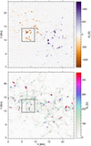 |
Fig. 1. Horizontal distributions of the longitudinal (BL; top panel) and horizontal (BH; bottom panel) components of the magnetic field at optical depth of log (τ500) = 0. The black square indicates the region used in this study. |
3. Spectral synthesis
We employed the STiC code to synthesize the Stokes spectra of the Mg I 12.32 μm line from the 3D MHD simulation, using a spectral sampling of 0.05 nm within the wavelength range from 12315.16 nm to 12321.56 nm. The synthesis was conducted using a specific region of the simulation, as indicated by the black square in Fig. 1. The STiC code operates under the assumption of plane-parallel geometry, performing computations independently for each column of the simulation model. Additionally, the synthesis is carried out under complete frequency redistribution (CRD) conditions, assuming observations at the disk center (i.e., μ = 1, where μ = cos θ and θ is the heliocentric angle). Here, we derived the atomic parameters from the modified model atom MgI_66.atom, as described in Sedik et al. (2024).
We investigated the effect of noise on the Stokes profiles of the Mg I 12.32 μm line by adding random Gaussian noise to the four Stokes parameters at four different levels (σ) corresponding to values of 5 × 10⁻⁴, 1 × 10⁻³, 5 × 10⁻³, and 1 × 10⁻² relative to the continuum intensity (Ic). To illustrate the impact of this noise, Fig. 2 presents a filtergram of Stokes Q, U, and V at a wavelength of Δλ = −0.2 nm from the line center. It allows us to compare maps of Stokes profiles without noise to those with the four specified noise levels. As mentioned above, we did not incorporate any spectral degradation in this study. Consequently, the synthetic Stokes profiles of the Mg I 12.32 μm line display larger amplitudes than those from the observations (Hewagama et al. 1993; Jennings et al. 2002; Moran et al. 2007). However, we do note that a significant amount of polarization signals have amplitudes exceeding 1 × 10⁻² of Ic, as seen in the first row of Fig. 2.
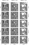 |
Fig. 2. Filtergram of Stokes Q (left column), U (middle column), and V (right column) at a wavelength Δλ = −0.2 nm from the line center of the Mg I 12.32 μm line. From top to bottom: Synthetic Stokes profiles and those with a random Gaussian noise of amplitudes 5 × 10⁻⁴, 1 × 10⁻³, 5 × 10⁻³, and 1 × 10⁻² relative to the mean continuum intensity Ic, respectively. |
As seen in the left and middle columns of Fig. 2, the linear polarization signals (Q and U) predominantly appear at the edges of strong field concentrations due to the horizontal expansion of magnetic field lines with height. Most magnetic features are clearly visible at noise levels of σ = 5 × 10⁻⁴ and 1 × 10⁻³ of Ic. However, at the higher noise levels, many weak signals become obscured by noise (particularly in the region around [3.5, 3] Mm). Nonetheless, some areas with strong signals remain detectable.
The Stokes V signals stand out above all noise levels, with the exception of two regions with weak signals located around [3.0, 2.5] Mm and [4.5, 2.7] Mm (see right column of Fig. 2). These strong signals are primarily located at the centers of strong field concentrations, where the field lines are highly vertical.
4. Inversions of the Stokes profiles
The inversions were performed using the STiC code for the synthetic profiles within the specified region of the Bifrost simulation (denoted by the black square in Fig. 1). We conducted inversions on both the original profiles and those with four different noise levels. To achieve the best fit to the Stokes profiles and obtain the most constrained atmospheric model, the inversions should be initialized with a variety of model atmospheres to help the code converge toward the global χ2 minimum. To reduce the computing time, we implemented single-cycle inversions initialized with one guess atmosphere. The initial atmosphere was the C model of Fontenla et al. (1993), to which we added a uniform magnetic field vector. Specifically, the longitudinal magnetic field component was set to 400 G, the horizontal component to 200 G, with a fixed field azimuth of 90°. The height range of the initial model is within log (τ500) = [1.4, −6.0]. Furthermore, we conducted inversions on a pixel-by-pixel basis, treating each spatial point independently.
The inversion configuration employed an equally distributed set of nodes along the atmospheric height for the physical parameters as follows: five nodes for temperature, four nodes for line-of-sight (LOS) velocity, and three nodes each for the longitudinal and horizontal magnetic field components, with a single node for field azimuth. We found this configuration provides accurate results, while maintaining an optimal number of degrees of freedom (nodes). Additionally, we did not include any microturbulence velocity in our inversions, given its absence in the Bifrost simulation.
4.1. Inversion of original profiles
We initially performed an inversion for the synthetic Stokes profiles without introducing any noise to evaluate the performance of the inversion process. We calculated the mean difference between the inferred atmospheric parameters and the original atmosphere of the Bifrost simulation, as illustrated in Fig. 3. For the temperature, the mean difference remains small across the hight range of log (τ500) = [−1.0, −3.0]. In contrast, for other atmospheric parameters, the mean difference is observed within the range of log (τ500) = [−2.0, −4.0]. The close agreement in temperature at relatively lower heights is attributed to its influence on the continuum intensity, which forms at approximately 200 km above the solar visible surface, as reported by Li et al. (2021). Furthermore, the minimum differences observed across all atmospheric parameters occur near an optical depth of log (τ500) = − 2.9. This optical depth corresponds to an average geometric height of approximately 450 km in the simulation, consistent with the sensitivity height of the Mg I 12.32 μm line (Chang et al. 1991; Carlsson & Rutten 1992).
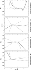 |
Fig. 3. Mean differences between the inferred atmospheric parameters and those of the simulation (solid line) as a function of the optical depth log (τ500). From top to bottom: Temperature, LOS velocity, and longitudinal and horizontal components of magnetic field. The dotted curves enclose the standard deviation of the differences. |
Figure 4 displays maps of the inferred atmospheric parameters derived from the inversion, compared to the original simulation atmosphere at an optical depth of log (τ500) = − 2.9. The inferred temperature exhibits a relatively good agreement with the simulation (first row of Fig. 4), resulting in a Pearson correlation coefficient of r = 0.82. The inferred LOS velocity closely aligns with the simulation (second row of Fig. 4), resulting in a Pearson correlation coefficient of r = 0.95.
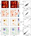 |
Fig. 4. Maps (from top to bottom): Temperature, LOS velocity, and longitudinal and horizontal magnetic field components from the simulation (left column) and inversion (middle column) at optical depth of log (τ500) = − 2.9. The scatter plots of each atmospheric parameter are presented in the right column, with the Pearson correlation coefficient (r) at the bottom right, and the red dashed lines represent one-to-one correspondences. The green numbers indicate selected pixels which their Stokes profiles are displayed in this work. |
The inferred longitudinal magnetic field component is in good agreement with the model (third row of Fig. 4), resulting in r = 0.99. While the inferred horizontal magnetic field component is generally close to the original atmosphere (fourth row of Fig. 4; r = 0.93), there are some clear differences.
Figure 5 presents the synthetic Stokes profiles along with their corresponding fits for three example pixels highlighted in Fig. 4. Pixel 1 is located in a region with a weak magnetic field, whereas pixels 2 and 3 correspond to regions with relatively strong longitudinal and horizontal magnetic fields, respectively. The inversion code successfully reproduces the two absorption troughs and the emission peak of Stokes I in pixel 1, as well as the double- and triple-lobed intensity profiles in pixels 2 and 3. Moreover, the fitting of Stokes Q, U, and V are good, particularly the complex Stokes V profile exhibiting four distinct lobes in pixel 2.
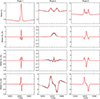 |
Fig. 5. Synthetic Stokes profiles (black) and their corresponding fits (red) for the three example pixels (columns) indicated in Fig. 4. |
4.2. Inversions of noisy profiles
We evaluate the influence of photon noise on the inferred atmospheric parameters by performing inversions of synthetic Stokes profiles with four different noise levels: 5 × 10⁻⁴, 1 × 10⁻³, 5 × 10⁻³, and 1 × 10⁻² relative to Ic. Figure 6 illustrates the inversion results for each noise level. The inferred temperature (left column) remains remarkably consistent with the original simulation atmosphere, even at the highest noise level of 1 × 10⁻².
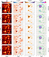 |
Fig. 6. Maps of the model’s and the inferred atmospheric parameters from the inversions of Stokes profiles with four different noise levels. From top to bottom: Original atmosphere, inversions results for noise levels of 5 × 10⁻⁴, 1 × 10⁻³, 5 × 10⁻³, and 1 × 10⁻² of Ic, as seen in the right part of the plots. Columns from left to right: Temperature, LOS velocity, and longitudinal and horizontal components of the magnetic field, respectively. |
The second and third columns of Fig. 6 present the LOS velocity and longitudinal component of the magnetic field, respectively. Both atmospheric parameters are in good agreement with those of the simulation. The inferred values exhibit small differences for noise levels higher than 1 × 10⁻³, whereas the strong longitudinal field features are still accurately recovered up to a noise level of 1 × 10⁻².
Regarding the horizontal component of the magnetic field (right column in Fig. 6), the inferred values are close to the original ones for noise levels up to 1 × 10⁻³ and the discrepancies become significantly large for the higher noise levels. Only regions with strong horizontal magnetic field could be determined with minor differences for noise levels up to 5 × 10⁻³.
To facilitate a detailed comparison, Fig. 7 presents histograms of the absolute differences between the inferred and simulated atmospheric parameters. The distribution of temperature differences shows a peak at zero for inversion results derived from the original spectra (i.e., without adding any noise σ = 0). As the noise levels increase, the distributions maintain a similar shape and width, with the peaks slightly decreasing at noise levels of 5 × 10⁻³ and 1 × 10⁻².
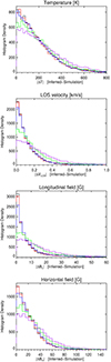 |
Fig. 7. Histograms of the absolute differences between the inferred atmospheric parameters and those of the Bifrost simulation at optical depth of log (τ500) = − 2.9. Black, red, blue, green, and purple colors correspond to the inversion results of Stoke profiles, without any noise and those with noise levels of 5 × 10⁻⁴, 1 × 10⁻³, 5 × 10⁻³, and 1 × 10⁻² of Ic, respectively. |
For the other atmospheric parameters (VLOS, BL, and BH), the histograms exhibit relatively narrow distributions with peaks centered at zero for the inversion results of the original spectra, indicating only slight differences between the inferred parameters and those in the original atmosphere. For noise levels up to 1 × 10⁻³, the distribution of differences has a similar shape. However, increasing noise levels lead to more pronounced differences. The peaks of these distributions rapidly decline, while their wings broaden, indicating a significant degradation in the accuracy of the inferred parameters for noise levels exceeding 1 × 10⁻³.
Overall, this analysis demonstrates the capability of inferring the atmospheric parameters from the inversion of Stokes profiles of the Mg I 12.32 μm line. Based on the Bifrost simulation, we found that the inversion can accurately retrieve the atmospheric parameters for observations with noise levels up to 1 × 10⁻³ of Ic.
5. Discussion and conclusions
In this study, we investigated the inversion of Stokes profiles for the Mg I 12.32 μm spectral line using a 3D MHD simulation, aiming to assess the accuracy of the retrieved atmospheric parameters. The Mg I 12.32 μm line is a powerful diagnostic tool for probing solar magnetic fields in the upper photosphere, owing to its high sensitivity to relatively weak magnetic fields and its clearly observable Zeeman splitting for BZ and/or BH exceeding 100 G and 300 G, respectively.
We employed the STiC code to synthesize and invert Stokes profiles from a snapshot of a Bifrost MHD simulation, focusing on a region with a wide range of magnetic field strengths. Furthermore, we examined the impact of four noise levels (5 × 10⁻⁴, 1 × 10⁻³, 5 × 10⁻³, and 1 × 10⁻² of Ic) on the inferred atmospheric parameters.
The minimum difference between the inferred and original atmospheres occurred at an optical depth of log (τ500) = − 2.9. The inversion could accurately retrieve atmospheric parameters for noise levels up to 1 × 10⁻³ of Ic, while the temperature was robustly reconstructed even at the highest noise level (1 × 10⁻² of Ic). However, the sensitivity of BL and BH to noise underscores the challenges in accurately inferring the magnetic field, particularly in regions with weak polarization signals. The findings are relevant for future large aperture solar telescopes, such as the Chinese Gaint Solar Telescope (CGST) with its eight-meter aperture, highlighting the need for high signal-to-noise observations to reliably diagnose weak polarization signal features of magnetic origin.
This study has certain limitations, notably the exclusion of spectral and spatial degradation effects that are inherent in actual observational data. Addressing these instrumental effects in future research would produce more realistic synthetic profiles. Additionally, employing multi-cycle inversions with varied initial models could improve the fitting quality of the Stokes profiles and enable the retrieval of a more constrained and reliable atmospheric model. Finally, our results advance our understanding of the diagnostic capabilities of the Mg I 12.32 μm line and validate spectropolarimetric inversions as a tool for interpreting solar magnetic field observations of this line under realistic noise conditions.
Acknowledgments
This work is supported by National Key R&D Program of China (2021YFA1600500), the Strategic Priority Research Program of the Chinese Academy of Sciences (grant No. XDB0560000), the Youth Innovation Promotion Association CAS (2023061), and the National Natural Sciences Foundation of China (NSFC, grant No. 12373058).
References
- Beck, C., Gosain, S., & Kiessner, C. 2019, ApJ, 878, 60 [NASA ADS] [CrossRef] [Google Scholar]
- Brault, J., & Noyes, R. 1983, ApJ, 269, L61 [Google Scholar]
- Carlsson, M., & Rutten, R. J. 1992, A&A, 259, L53 [NASA ADS] [Google Scholar]
- Carlsson, M., Hansteen, V. H., Gudiksen, B. V., Leenaarts, J., & De Pontieu, B. 2016, A&A, 585, A4 [NASA ADS] [CrossRef] [EDP Sciences] [Google Scholar]
- Chang, E. S., Avrett, E. H., Mauas, P. J., Noyes, R. W., & Loeser, R. 1991, ApJ, 379, L79 [Google Scholar]
- da Silva Santos, J. M., de la Cruz Rodríguez, J., & Leenaarts, J. 2018, A&A, 620, A124 [NASA ADS] [CrossRef] [EDP Sciences] [Google Scholar]
- de la Cruz Rodríguez, J., & van Noort, M. 2017, Space Sci. Rev., 210, 109 [Google Scholar]
- de la Cruz Rodríguez, J., Socas-Navarro, H., Carlsson, M., & Leenaarts, J. 2012, A&A, 543, A34 [Google Scholar]
- de la Cruz Rodríguez, J., Leenaarts, J., & Asensio Ramos, A. 2016, ApJ, 830, L30 [Google Scholar]
- de la Cruz Rodríguez, J., Leenaarts, J., Danilovic, S., & Uitenbroek, H. 2019, A&A, 623, A74 [Google Scholar]
- del Toro Iniesta, J. C., & Ruiz Cobo, B. 2016, Liv. Rev. Sol. Phys., 13, 4 [Google Scholar]
- Deng, Y., Wang, D., Hua, J., et al. 2025, RAA, 25, 075020 [Google Scholar]
- Fontenla, J. M., Avrett, E. H., & Loeser, R. 1993, ApJ, 406, 319 [Google Scholar]
- Gudiksen, B. V., Carlsson, M., Hansteen, V. H., et al. 2011, A&A, 531, A154 [NASA ADS] [CrossRef] [EDP Sciences] [Google Scholar]
- Hewagama, T., Deming, D., Jennings, D. E., et al. 1993, ApJS, 86, 313 [Google Scholar]
- Jennings, D. E., Deming, D., McCabe, G., Sada, P. V., & Moran, T. 2002, ApJ, 568, 1043 [NASA ADS] [CrossRef] [Google Scholar]
- Landi Degl’Innocenti, E., & Landolfi, M. 2004, Polarization in Spectral Lines (Dordrecht: Kluwer Academic Publishers), 307 [Google Scholar]
- Li, X., Song, Y., Uitenbroek, H., et al. 2021, A&A, 646, A79 [NASA ADS] [CrossRef] [EDP Sciences] [Google Scholar]
- Lites, B. W., Kubo, M., Socas-Navarro, H., et al. 2008, ApJ, 672, 1237 [Google Scholar]
- Martínez González, M. J., & Bellot Rubio, L. R. 2009, ApJ, 700, 1391 [CrossRef] [Google Scholar]
- Moran, T. G., Jennings, D. E., Deming, L. D., et al. 2007, Sol. Phys., 241, 213 [NASA ADS] [CrossRef] [Google Scholar]
- Murcray, F. J., Goldman, A., Murcray, F. H., et al. 1981, ApJ, 247, L97 [Google Scholar]
- Sedik, M., Bai, X., Li, W., Yang, X., & Deng, Y. 2024, A&A, 686, A278 [NASA ADS] [CrossRef] [EDP Sciences] [Google Scholar]
- Uitenbroek, H. 2001, ApJ, 557, 389 [Google Scholar]
All Figures
|
Fig. 1. Horizontal distributions of the longitudinal (BL; top panel) and horizontal (BH; bottom panel) components of the magnetic field at optical depth of log (τ500) = 0. The black square indicates the region used in this study. |
| In the text | |
|
Fig. 2. Filtergram of Stokes Q (left column), U (middle column), and V (right column) at a wavelength Δλ = −0.2 nm from the line center of the Mg I 12.32 μm line. From top to bottom: Synthetic Stokes profiles and those with a random Gaussian noise of amplitudes 5 × 10⁻⁴, 1 × 10⁻³, 5 × 10⁻³, and 1 × 10⁻² relative to the mean continuum intensity Ic, respectively. |
| In the text | |
|
Fig. 3. Mean differences between the inferred atmospheric parameters and those of the simulation (solid line) as a function of the optical depth log (τ500). From top to bottom: Temperature, LOS velocity, and longitudinal and horizontal components of magnetic field. The dotted curves enclose the standard deviation of the differences. |
| In the text | |
|
Fig. 4. Maps (from top to bottom): Temperature, LOS velocity, and longitudinal and horizontal magnetic field components from the simulation (left column) and inversion (middle column) at optical depth of log (τ500) = − 2.9. The scatter plots of each atmospheric parameter are presented in the right column, with the Pearson correlation coefficient (r) at the bottom right, and the red dashed lines represent one-to-one correspondences. The green numbers indicate selected pixels which their Stokes profiles are displayed in this work. |
| In the text | |
|
Fig. 5. Synthetic Stokes profiles (black) and their corresponding fits (red) for the three example pixels (columns) indicated in Fig. 4. |
| In the text | |
|
Fig. 6. Maps of the model’s and the inferred atmospheric parameters from the inversions of Stokes profiles with four different noise levels. From top to bottom: Original atmosphere, inversions results for noise levels of 5 × 10⁻⁴, 1 × 10⁻³, 5 × 10⁻³, and 1 × 10⁻² of Ic, as seen in the right part of the plots. Columns from left to right: Temperature, LOS velocity, and longitudinal and horizontal components of the magnetic field, respectively. |
| In the text | |
|
Fig. 7. Histograms of the absolute differences between the inferred atmospheric parameters and those of the Bifrost simulation at optical depth of log (τ500) = − 2.9. Black, red, blue, green, and purple colors correspond to the inversion results of Stoke profiles, without any noise and those with noise levels of 5 × 10⁻⁴, 1 × 10⁻³, 5 × 10⁻³, and 1 × 10⁻² of Ic, respectively. |
| In the text | |
Current usage metrics show cumulative count of Article Views (full-text article views including HTML views, PDF and ePub downloads, according to the available data) and Abstracts Views on Vision4Press platform.
Data correspond to usage on the plateform after 2015. The current usage metrics is available 48-96 hours after online publication and is updated daily on week days.
Initial download of the metrics may take a while.