| Issue |
A&A
Volume 701, September 2025
|
|
|---|---|---|
| Article Number | L11 | |
| Number of page(s) | 7 | |
| Section | Letters to the Editor | |
| DOI | https://doi.org/10.1051/0004-6361/202556329 | |
| Published online | 19 September 2025 | |
Letter to the Editor
Blowing star formation away in AGN hosts (BAH)
III. Serendipitous discovery of a z ∼ 2.9 star-forming galaxy lensed by the galactic bulge of CGCG 012-070 using JWST NIRSpec
1
Centro de Astrobiología (CAB), CSIC-INTA, Ctra. de Ajalvir km 4, Torrejón de Ardoz, E-28850 Madrid, Spain
2
Departamento de Física, CCNE, Universidade Federal de Santa Maria, Av. Roraima 1000, 97105-900 Santa Maria, RS, Brazil
3
Departamento de Astronomia, IF, Universidade Federal do Rio Grande do Sul, CP 15051, 91501-970 Porto Alegre, RS, Brazil
4
Departamento de Física, IF, Universidade Federal do Rio Grande do Sul, CP 15051, 91501-970 Porto Alegre, RS, Brazil
5
Department of Physics & Astronomy, Johns Hopkins University, Bloomberg Ctr, 3400 N. Charles St, Baltimore, MD 21218, USA
6
Department of Physics and Astronomy, 4129 Frederick Reines Hall, University of California, Irvine, CA 92697, USA
⋆ Corresponding author.
Received:
9
July
2025
Accepted:
1
September
2025
Abstract
We report the detection of a gravitationally lensed galaxy by the nearby spiral galaxy CGCG 012-070 (z = 0.048) using integral field unit (IFU) observations with the Near-Infrared Spectrograph (NIRSpec) instrument on board the James Webb Space Telescope (JWST). The lensed galaxy is identified through the flux distributions of emission lines in the rest-frame optical, consistent with a source located at a redshift of z ∼ 2.89. The system is detected in [O III] λλ4959, 5007, Hβ, and Hα emission lines, exhibiting line ratios typical of a star-forming galaxy. The emission-line flux distributions reveal three distinct components, which are modeled using an elliptical power-law mass profile for the lens galaxy. This model provides a good characterization of the source and reveals a disturbed star-forming morphology consistent with those of galaxies at cosmic noon. This serendipitous discovery of a rare low-redshift strong lens highlights the critical role of IFU observations in expanding the lens census and advancing our understanding of galaxy mass profiles and evolution.
Key words: gravitational lensing: strong / galaxies: active / galaxies: kinematics and dynamics / galaxies: spiral
© The Authors 2025
 Open Access article, published by EDP Sciences, under the terms of the Creative Commons Attribution License (https://creativecommons.org/licenses/by/4.0), which permits unrestricted use, distribution, and reproduction in any medium, provided the original work is properly cited.
This article is published in open access under the Subscribe to Open model. This email address is being protected from spambots. You need JavaScript enabled to view it. to support open access publication.
1. Introduction
Strong gravitational lensing occurs when the light from a distant background galaxy is distorted and magnified by the gravitational field of a foreground lens galaxy or galaxy cluster, aligned along the line of sight. This effect may produce multiple images or arcs of the background galaxy, with Einstein rings forming in cases of perfect alignment (e.g., Walsh et al. 1979; Saha et al. 2024). Strong gravitational lenses can provide valuable insights into the distribution of dark matter in galaxies and clusters (e.g., Tyson et al. 1998; Barnabè et al. 2012) and the detection and characterization of high-redshift objects (e.g., Dye et al. 2018; Chirivì et al. 2020; Yue et al. 2023; Abdurro’uf et al. 2024), constrain cosmological parameters (e.g., Refsdal 1964; Shajib et al. 2020), and enable us to estimate the mass of supermassive black holes (e.g., Nightingale et al. 2023; Melo-Carneiro et al. 2025), among other matters.
The detection of strong gravitational lenses often involves several technical challenges, such as managing large imaging datasets and designing tools for precise identification (e.g., Metcalf et al. 2019). The number of identified gravitational lenses has been increasing rapidly due to the recent launch of the Euclid space telescope (Euclid Collaboration: Mellier et al. 2025) and is expected to continue to grow, thanks to surveys such as the Legacy Survey of Space and Time (LSST; Ivezić et al. 2019). Gravitational lenses are found mainly in early-type galaxies, with only 10–20% in spirals (Auger et al. 2009), due to their lower mass and less concentrated mass distribution. Strong lenses produced by low-redshift spiral galaxies (z ≲ 0.1) are even more uncommon (Treu et al. 2011; O’Riordan et al. 2025). Gravitational lenses in low-redshift galaxies are particularly insightful as the lensed arcs are observed in the central region of the galaxy, where the lensing primarily traces stellar mass. This, in turn, can be used as an independent constraint on the initial mass function (IMF) mismatch parameter (e.g., Newman et al. 2017).
Here, we report the serendipitous detection of a strongly lensed galaxy by the spiral galaxy CGCG012-070 (z = 0.048), using observations taken with the Near-Infrared Spectrograph (NIRSpec) of the James Webb Space Telescope (JWST) in integral field unit (IFU) spectroscopy mode. This paper is structured as follows. Section 2 describes the observations and data reduction. Section 3 presents the main results, followed by a discussion in Sect. 4. Finally, the conclusions and their implications are summarized in Sect. 5.
2. Observations and data reduction
CGCG012-070 is a nearly edge-on (i ≈ 70°) Sb galaxy and hosts a Seyfert 2 active galactic nucleus (AGN; Kautsch et al. 2006; Véron-Cetty & Véron 2006). It was observed as part of the Blowing Star Formation Away in AGN Hosts (BAH; Costa-Souza et al. 2024; Riffel et al. 2025) project (PID: 1928, PI: Riffel, R. A.) using the JWST/NIRSpec instrument in the IFU mode (Böker et al. 2022). The observations were performed using the G235H filter in combination with the F170LP grating. We processed the data using the JWST Science Calibration Pipeline (Bushouse et al. 2024), version 1.12.5, and the reference file jwst_1183.pmap, following the standard pipeline stages. See de Mellos et al. (2025) for details.
3. Results
Through visual inspection of the NIRSpec data cube, we identified three components that are associated not with the galaxy but rather with a background object. These components were detected through the Hβ, [O III]λλ4959, 5007, and Hα emission lines. The top panels of Fig. 1 display the observed flux distributions for [O III]λ5007 and Hα, along with a composite image combining the [O III]λ5007 emission (in red) and the continuum image of CGCG 012-070 (in green). The emission line maps were obtained by directly integrating the line profiles over velocity windows of 1500 km s−1, after subtracting the stellar population contribution obtained using the pPXF code (Cappellari 2023) in combination with the E-MILES templates (Vazdekis et al. 2016). Only spaxels where lines are detected with signal-to-noise ratio (S/N) of > 5 are shown and components are labeled A, B, and C in the [O III]λ5007 flux map. Component A exhibits an arc-shaped emission, whereas components B and C appear more point-like. The bottom panel of Fig. 1 shows the integrated spectrum for for component A. The insets highlight the regions around the emission lines of the background object. The emission lines [Fe II]1.8298 μm and H22.4237 μm, from the foreground galaxy, are also labeled. These emission lines do not affect the flux measurements of the background object’s lines, as they are outside the integration spectral windows. The spectra for the other two components are shown in Fig. B.1.
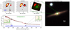 |
Fig. 1. Right panel: Composite image of CGCG 012-070 obtained from the Pan-STARRS archive (Chambers et al. 2016), covering a region of 60 × 60 arcsec2. The image combines the r, i, and z bands. The green square indicates the NIRSpec field of view, which encompasses the inner region of the galaxy’s bulge. Small top panels: [O III] λ5007 (left) and Hα (center) flux maps for the z ∼ 2.89 lensed object, and a composite image (right), with the image of the lensed object shown in red and the 2.0 μm continuum image of the galaxy CGCG 012-070 in green. Bottom panel: Spectrum at the position of the lensed component A, identified in the top left panel. The observed spectrum is shown in black, the stellar population contribution of CGCG 012-070 in red, and the gas component in blue. The insets provide a zoom-in on the [O III] and Hα regions for the lensed object. The [Fe II] and H2 labels, identified in black, represent Fe and H2 lines from the foreground galaxy. |
The emission components of the background source closely resemble those of strong gravitational lenses observed in other galaxies (e.g., Treu et al. 2011; Galbany et al. 2018; Euclid Collaboration: Walmsley et al. 2025; Euclid Collaboration: Rojas et al. 2025), supporting their interpretation as such. Using the spectra of these components, we estimated the redshift for each one based on the emission lines. Using the [O III]λ5007 line, we derive redshifts of 2.8871, 2.8869, and 2.8844 for components A, B, and C, respectively. Similarly, from the Hα line, we estimate redshifts of 2.8872 and 2.8873 for components A and B. The mean redshift is ⟨z⟩ = 2.8866 ± 0.0011, where the uncertainty represents the standard deviation of the mean.
4. Discussion
Because of its prominence, we modeled the [O III]λ5007 lensed emission using an elliptical power-law (EPL) mass profile for the lens galaxy, as implemented in PyAutoLens (Nightingale et al. 2018, 2021), and with the inclusion of an external shear. Before the modeling, we added background noise sampled from a normal distribution with a zero mean and a dispersion of σ15 = 15% of the peak arc brightness, in regions where there is no [O III]λ5007 detection (Dutton et al. 2011; Barnabè et al. 2012). Such noise is intended to suppress models that predict significant lensed features elsewhere. We assumed the uncertainty in this region to be equal to σ15, and we estimated the uncertainty in the [O III]λ5007 by assuming a Gaussian noise distribution. More details about the modeling strategy and systematic tests are presented in Appendix C.
Figure 2 displays the highest-likelihood lens model, the normalized residuals, and the reconstructed [O III]λ5007 source in the upper panels. The model accurately fits the data, particularly component A, which exhibits a higher S/N. Despite the overall success, significant, structured residuals are evident for component B and at the outer edges of component A. We hypothesize that this may be caused by the high elongation of the projected mass profile of the lensing disk galaxy, which a single EPL profile cannot fully capture. An EPL model is known to be insufficient in reproducing the “disky” isodensity contours (i.e., higher-order multipole moments) of a stellar disk. The impact of this model mismatch is most pronounced for component B, as its location within the tangential critical curve makes its morphology more sensitive to complexities in the mass distribution that our model may lack. To develop more physically motivated models, such as a multicomponent mass decomposition (e.g., Barnabè et al. 2012), higher-quality imaging data would be necessary. We then used the same mask and mass model from this fit to reconstruct the Hα emission1, which we show in the bottom panel of Fig. 2. We found an effective Einstein radius for the EPL model, defined as the radius of a circle with the same area enclosed by the tangential critical curve, of  arcsec (∼1.8 kpc), which corresponds to a total mass within it of
  . This value is consistent with the one we estimate from stellar population synthesis for the lens galaxy, of M⋆(M⊙/1010) = 6.88 ± 0.89, following Riffel et al. (2024). This results in an estimated dark matter fraction of ∼12% within REin, consistent with other low-z lens galaxies (e.g., Newman et al. 2017; Collett et al. 2018). We also estimate the lensing magnification factor as ∼1.18.
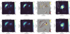 |
Fig. 2. Highest-likelihood EPL lens model. Each row illustrates a different emission line. From left to right, we present the modified (noise-added) observed image, the model image, the normalized residuals, and the reconstructed source. The top row details the [O III]λ5007 results, whereas the bottom row displays the Hα reconstruction, utilizing the mass model obtained from fitting the [O III]λ5007 emission. Fluxes are in units of 10−18 erg s cm−2. |
The reconstructed [O III]λ5007 image has a disturbed morphology. Components A and B are traced to the same spatial location in the source plane, which indicates that they correspond to an image and its counterimage. This interpretation is supported by the [O III]λ5007 velocity measurements, which show similar values for these components. Component C is traced back to a different location in the source plane (white ellipse) and shows a [O III]λ5007 velocity ∼250 km s−1 blueshifted relative to components A and B. Additionally, it is important to note that component C is unresolved and is detected only marginally. Despite tracing distinct galaxy components, such as gas rather than stars, this type of disturbed morphology is commonly observed in other lensed cosmic noon galaxies (Jones et al. 2010; Dye et al. 2015).
Using the fluxes of the emission lines measured in an integrated spectrum, summing the components A and B, we obtain log[O III]λ5007/Hβ = 0.71 ± 0.08. Although the [N II]6583 emission line is not detected, we can set an upper limit of log[N II]λ6583/Hα < −1.1. These values are consistent with emission originating from photoionization by young stars (Kewley et al. 2001; Kauffmann et al. 2003), indicating that the background object is a star-forming galaxy. This is also consistent with the disturbed morphology of the gas distribution in the reconstructed source, as discussed above. Using the Hα luminosity, corrected for lensing magnification, and the relation from Kennicutt (1998), we estimate a star formation rate of SFR ∼ 70 M⊙ yr−1, which is consistent with measurements reported for galaxies at similar redshifts (e.g., Förster Schreiber et al. 2009).
Discovering strong galaxy-scale gravitational lenses remains challenging in ground-based surveys due to limitations imposed by atmospheric seeing. As a result, only a relatively small number of lenses were identified in the Sloan Digital Sky Survey (Bolton et al. 2006, 2008). In contrast, space-based missions such as Euclid are now uncovering vast numbers of lenses (Euclid Collaboration: Walmsley et al. 2025; Euclid Collaboration: Rojas et al. 2025), and the upcoming Nancy Grace Roman Space Telescope is expected to identify even more (Weiner et al. 2020; Wedig et al. 2025). These efforts make it increasingly clear that the current census of single-galaxy lenses is still far from complete. Serendipitous discoveries with the JWST, particularly using its IFU capabilities, fill a unique observational niche. The spatial resolution and, crucially, the high contrast achievable within a very narrow spectral band allow for the detection of lenses with Einstein radii comparable to or smaller than the bulge of the lensing galaxy. Such lenses are next to impossible to identify in broad-band imaging surveys. Such discoveries, although incidental, are crucial for expanding the sample of known lenses and for addressing key statistical questions, such as distinguishing between substructure lensing and line-of-sight halo contributions (e.g., Sengül et al. 2022).
The lens reported here is produced by a low-redshift galaxy, a class of systems that is extremely rare. The probability of a galaxy at z ∼ 0.05 producing a detectable strong lens is estimated at only 1 in 2000, so even wide-area surveys such as Euclid are expected to find just a few (4–20) such systems (O’Riordan et al. 2025). To date, only five strong lensing systems with lens galaxies at z < 0.05 have been identified, including the one presented here, which is the second hosted by a spiral galaxy. Its lensed source is the most distant among those associated with low-redshift lenses (Table D.1). Discovering and building a census of strong lenses at very low redshifts is crucial for anchoring models of galaxy evolution, as such systems enable direct measurements of inner mass profiles on kiloparsec scales and provide key constraints on cosmological predictions for the redshift evolution of galaxy density slopes (Sahu et al. 2024). This underscores both the rarity and the significance of discovering a low-redshift lens through serendipitous IFU observations.
5. Conclusions
This work presents a remarkable discovery of a gravitational lens system with JWST, confirming the origin of its lensed [O III]λ5007 and Hα emissions. We estimate a redshift of z ≈ 2.89 background source based on the central wavelengths of the observed emission lines. Additionally, the intensity ratios of these lines indicate that the primary ionization source of the gas is star formation. We modeled the lens system using an EPL profile, which effectively identified components A and B as a confirmed image and its counterimage. Furthermore, the model revealed a disturbed, star-forming source morphology consistent with cosmic noon galaxies. While our model provides a strong initial characterization, future deep imaging and spectroscopy will enable more detailed investigations of the lens and source objects, including constraints on the IMF, and will also allow us to combine lens kinematics to precisely separate stellar and dark matter contributions within the lens galaxy.
For this purpose, we kept the mass model fixed and sampled only the source-plane pixelization and regularization parameters.
Additional details are available in the online documentation for PyAutoLens: https://github.com/Jammy2211/autolens_workspace.
Acknowledgments
This work is based on observations made with the NASA/ESA/CSA James Webb Space Telescope. The data were obtained from the Mikulski Archive for Space Telescopes (MAST) at the Space Telescope Science Institute, which is operated by the Association of Universities for Research in Astronomy, Inc., under NASA contract NAS 5-03127 for JWST. These observations are associated with program #1928. The complete dataset can be accessed at MAST platform, through https://doi.org/10.17909/tazj-hp44. We thank the referee for valuable suggestions. ChatGPT (GPT-4.5) was used to improve sentence wording. RAR, GLSO, JHCS and MZM acknowledge the support from the Conselho Nacional de Desenvolvimento Científico e Tecnológico (CNPq; Projects 303450/2022-3, 403398/2023-1, and 441722/2023-7) and the Coordenação de Aperfeiçoamento de Pessoal de Nível Superior (CAPES; Project 88887.894973/2023-00, and Finance code 0001). RR acknowledges support from CNPq (Proj. 445231/2024-6,311223/2020-6, 404238/2021-1, and 310413/2025-7), FAPERGS, (Proj. 19/1750-2 and 24/2551-0001282-6) and CAPES (88881.109987/2025-01). CF acknowledges the support from CNPq Project 315421/2023-1. ACS acknowledges support from FAPERGS (grants 23/2551-0001832-2 and 24/2551-0001548-5), CNPq (grants 314301/2021-6, 312940/2025-4, 445231/2024-6, and 404233/2024-4), and CAPES (grant 88887.004427/2024-00).
References
- Abdurro’uf, Larson, R. L., Coe, D., et al. 2024, ApJ, 973, 47 [Google Scholar]
- Adelman-McCarthy, J. K., Agüeros, M. A., Allam, S. S., et al. 2008, ApJS, 175, 297 [NASA ADS] [CrossRef] [Google Scholar]
- Auger, M. W., Treu, T., Bolton, A. S., et al. 2009, ApJ, 705, 1099 [Google Scholar]
- Barnabè, M., Dutton, A. A., Marshall, P. J., et al. 2012, MNRAS, 423, 1073 [Google Scholar]
- Böker, T., Arribas, S., Lützgendorf, N., et al. 2022, A&A, 661, A82 [NASA ADS] [CrossRef] [EDP Sciences] [Google Scholar]
- Bolton, A. S., Burles, S., Koopmans, L. V. E., Treu, T., & Moustakas, L. A. 2006, ApJ, 638, 703 [NASA ADS] [CrossRef] [Google Scholar]
- Bolton, A. S., Burles, S., Koopmans, L. V. E., et al. 2008, ApJ, 682, 964 [Google Scholar]
- Bushouse, H., Eisenhamer, J., Dencheva, N., et al. 2024, https://doi.org/10.5281/zenodo.10870758 [Google Scholar]
- Cao, X., Li, R., Nightingale, J. W., et al. 2022, Res. Astron. Astrophys., 22, 025014 [CrossRef] [Google Scholar]
- Cappellari, M. 2023, MNRAS, 526, 3273 [NASA ADS] [CrossRef] [Google Scholar]
- Chambers, K. C., Magnier, E. A., Metcalfe, N., et al. 2016, arXiv e-prints [arXiv:1612.05560] [Google Scholar]
- Chirivì, G., Yıldırım, A., Suyu, S. H., & Halkola, A. 2020, A&A, 643, A135 [EDP Sciences] [Google Scholar]
- Collett, T. E., Oldham, L. J., Smith, R. J., et al. 2018, Science, 360, 1342 [CrossRef] [Google Scholar]
- Costa-Souza, J. H., Riffel, R. A., Souza-Oliveira, G. L., et al. 2024, ApJ, 974, 127 [Google Scholar]
- de Mellos, M. S. Z., Riffel, R. A., Souza-Oliveira, G. L., et al. 2025, arXiv e-prints [arXiv:2506.20896] [Google Scholar]
- Dutton, A. A., Brewer, B. J., Marshall, P. J., et al. 2011, MNRAS, 417, 1621 [NASA ADS] [CrossRef] [Google Scholar]
- Dye, S., Furlanetto, C., Swinbank, A. M., et al. 2015, MNRAS, 452, 2258 [NASA ADS] [CrossRef] [Google Scholar]
- Dye, S., Furlanetto, C., Dunne, L., et al. 2018, MNRAS, 476, 4383 [Google Scholar]
- Etherington, A., Nightingale, J. W., Massey, R., et al. 2022, MNRAS, 517, 3275 [CrossRef] [Google Scholar]
- Euclid Collaboration (Mellier, Y., et al.) 2025, A&A, 697, A1 [Google Scholar]
- Euclid Collaboration (Rojas, K., et al.) 2025, A&A, in press, https://doi.org/10.1051/0004-6361/202554605 [Google Scholar]
- Euclid Collaboration (Walmsley, M., et al.) 2025, A&A, submitted [arXiv:2503.15324] [Google Scholar]
- Förster Schreiber, N. M., Genzel, R., Bouché, N., et al. 2009, ApJ, 706, 1364 [Google Scholar]
- Galbany, L., Collett, T. E., Méndez-Abreu, J., et al. 2018, MNRAS, 479, 262 [NASA ADS] [CrossRef] [Google Scholar]
- Huchra, J., Gorenstein, M., Kent, S., et al. 1985, AJ, 90, 691 [NASA ADS] [CrossRef] [Google Scholar]
- Ivezić, Ž., Kahn, S. M., Tyson, J. A., et al. 2019, ApJ, 873, 111 [Google Scholar]
- Jones, T. A., Swinbank, A. M., Ellis, R. S., Richard, J., & Stark, D. P. 2010, MNRAS, 404, 1247 [NASA ADS] [Google Scholar]
- Kauffmann, G., Heckman, T. M., Tremonti, C., et al. 2003, MNRAS, 346, 1055 [Google Scholar]
- Kautsch, S. J., Grebel, E. K., Barazza, F. D., & Gallagher, J. S. I. 2006, A&A, 445, 765 [NASA ADS] [CrossRef] [EDP Sciences] [Google Scholar]
- Kennicutt, R. C., Jr 1998, ARA&A, 36, 189 [NASA ADS] [CrossRef] [Google Scholar]
- Kewley, L. J., Dopita, M. A., Sutherland, R. S., Heisler, C. A., & Trevena, J. 2001, ApJ, 556, 121 [Google Scholar]
- Melo-Carneiro, C. R., Furlanetto, C., & Chies-Santos, A. L. 2025, JCAP, 2025, 046 [Google Scholar]
- Meneghetti, M., Bartelmann, M., Dahle, H., & Limousin, M. 2013, Space Sci. Rev., 177, 31 [NASA ADS] [CrossRef] [Google Scholar]
- Metcalf, R. B., Meneghetti, M., Avestruz, C., et al. 2019, A&A, 625, A119 [NASA ADS] [CrossRef] [EDP Sciences] [Google Scholar]
- Newman, A. B., Smith, R. J., Conroy, C., Villaume, A., & van Dokkum, P. 2017, ApJ, 845, 157 [NASA ADS] [CrossRef] [Google Scholar]
- Nightingale, J. W., Dye, S., & Massey, R. J. 2018, MNRAS, 478, 4738 [Google Scholar]
- Nightingale, J., Hayes, R., Kelly, A., et al. 2021, J. Open Source Software, 6, 2825 [NASA ADS] [CrossRef] [Google Scholar]
- Nightingale, J. W., Smith, R. J., He, Q., et al. 2023, MNRAS, 521, 3298 [NASA ADS] [CrossRef] [Google Scholar]
- O’Riordan, C. M., Oldham, L. J., Nersesian, A., et al. 2025, A&A, 694, A145 [NASA ADS] [CrossRef] [EDP Sciences] [Google Scholar]
- Perrin, M. D., Soummer, R., Elliott, E. M., Lallo, M. D., & Sivaramakrishnan, A. 2012, in Space Telescopes and Instrumentation 2012: Optical, Infrared, and Millimeter Wave, eds. M. C. Clampin, G. G. Fazio, & H. A. MacEwen, SPIE Conf. Ser., 8442, 84423D [Google Scholar]
- Planck Collaboration XIII. 2016, A&A, 594, A13 [NASA ADS] [CrossRef] [EDP Sciences] [Google Scholar]
- Refsdal, S. 1964, MNRAS, 128, 307 [NASA ADS] [CrossRef] [Google Scholar]
- Riffel, R., Dahmer-Hahn, L. G., Vazdekis, A., et al. 2024, MNRAS, 531, 554 [CrossRef] [Google Scholar]
- Riffel, R. A., Souza-Oliveira, G. L., Costa-Souza, J. H., et al. 2025, ApJ, 982, 69 [Google Scholar]
- Saha, P., Sluse, D., Wagner, J., & Williams, L. L. R. 2024, Space Sci. Rev., 220, 12 [NASA ADS] [CrossRef] [Google Scholar]
- Sahu, N., Tran, K.-V., Suyu, S. H., et al. 2024, ApJ, 970, 86 [CrossRef] [Google Scholar]
- Sengül, A. Ç., Dvorkin, C., Ostdiek, B., & Tsang, A. 2022, MNRAS, 515, 4391 [CrossRef] [Google Scholar]
- Shajib, A. J., Birrer, S., Treu, T., et al. 2020, MNRAS, 494, 6072 [Google Scholar]
- Sibson, R. 1981, in Interpreting Multivariate Data, ed. V. Barnett (New York: John Wiley& Sons), 21 [Google Scholar]
- Smith, R. J., Lucey, J. R., & Conroy, C. 2015, MNRAS, 449, 3441 [Google Scholar]
- Speagle, J. S. 2020, MNRAS, 493, 3132 [Google Scholar]
- Tessore, N., & Metcalf, R. B. 2015, A&A, 580, A79 [NASA ADS] [CrossRef] [EDP Sciences] [Google Scholar]
- Treu, T., Dutton, A. A., Auger, M. W., et al. 2011, MNRAS, 417, 1601 [Google Scholar]
- Trott, C. M., Treu, T., Koopmans, L. V. E., & Webster, R. L. 2010, MNRAS, 401, 1540 [NASA ADS] [CrossRef] [Google Scholar]
- Tyson, J. A., Kochanski, G. P., & Dell’Antonio, I. P. 1998, ApJ, 498, L107 [Google Scholar]
- Vazdekis, A., Koleva, M., Ricciardelli, E., Röck, B., & Falcón-Barroso, J. 2016, MNRAS, 463, 3409 [Google Scholar]
- Véron-Cetty, M. P., & Véron, P. 2006, A&A, 455, 773 [Google Scholar]
- Walsh, D., Carswell, R. F., & Weymann, R. J. 1979, Nature, 279, 381 [Google Scholar]
- Wedig, B., Daylan, T., Birrer, S., et al. 2025, ApJ, 986, 42 [Google Scholar]
- Weiner, C., Serjeant, S., & Sedgwick, C. 2020, Res. Notes Am. Astron. Soc., 4, 190 [Google Scholar]
- Yue, M., Fan, X., Yang, J., & Wang, F. 2023, AJ, 165, 191 [NASA ADS] [CrossRef] [Google Scholar]
Appendix A: The lens galaxy: CGCG012-070
In Fig. A.1 we present an image of the continuum at 2.0 μm extracted from the NIRSpec data cube, along with flux maps for the [Fe II]1.6440μm, Paα, and H22.1218 μm emission lines. These maps were created by integrating the spectra over a 1500 kms−1 window centered on each emission line, after subtracting stellar population contribution obtained using the pPXF code (Cappellari 2023) in combination with the E-MILES templates (Vazdekis et al. 2016). The bottom panel shows the integrated nuclear spectrum integrated within a 0 25 radius aperture in black, while the underlying stellar continuum is shown in red and the gas emission spectrum is shown in blue. The continuum image follows the same orientation as the large-scale disc, elongated along position angle PA≈107° (Adelman-McCarthy et al. 2008). The emission-line flux distributions peak at the galaxy’s nucleus, with weaker extended emission detected up to ∼2″ from it. The investigation of the origin of gas emission and kinematics is beyond the scope of this paper and will be addressed in a forthcoming study.
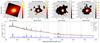 |
Fig. A.1. CGCG 012-070 galaxy. Top left panel: 2.0μm continuum image of CGCG 012-070, obtained from the NIRSpec data cube. Other top panels: Flux distributions of the [Fe II]1.6440μm, Paα, and H22.1218 μm emission lines. Gray regions represent masked out areas where the S/N < 3 and regions outside the NIRSpec FoV. The cross marks the position of the continuum peak. Bottom panel: Observed spectrum (in black), integrated over a 0 |

Appendix B: Spectra of components B and C
Figure B.1 shows the integrated spectra (in black) of the lensed components B and C, along with the corresponding stellar population models (in red) for CGCG 012-070. The residual spectra, shown in blue, were obtained by subtracting the stellar contribution from the integrated spectra. All observed spectra were extracted by summing the spaxels where the [O III] emission line is detected with S/N > 5 in each component, identified in Fig. 1.
 |
Fig. B.1. Integrated spectra for components B (top) and C (bottom). In each panel, the observed spectrum is shown in black, the stellar population contribution of CGCG 012-070 in red, and the gas component in blue. The insets provide a zoom-in on the [O III] and Hα regions for the lensed object. The [Fe II] and H2 labels identify emission lines from the foreground galaxy. |
Appendix C: Some details of the lens modeling
We performed the modeling using the open source lens modeling package PyAutoLens (Nightingale et al. 2018). Our approach utilized the SLaM (Source, Light, and Mass) pipelines distributed with PyAutoLens, similar to the methods employed in other works (e.g., Cao et al. 2022; Etherington et al. 2022), but with modifications to match our data. The pipeline workflow is summarized below:
-
Initialize: We began by creating a basic model for the lens mass and source light distribution using parametric profiles. The lens mass is assumed to be a singular isothermal ellipsoid (SIE)+shear, and the source’s brightness was modeled by a Sersic component.
-
Lens refinement and source pixelization: Using the results from the initial step, we re-sampled the lens mass model parameters alongside a pixelized source model. We employed a Voronoi mesh grid with Natural Neighbor interpolation (Sibson 1981) and brightness-adaptive regularization to smooth the reconstruction based on source luminosity. Priors on the mass parameters were updated using PyAutoLens’s default prior passing2.
-
Source pixelization refinement: We refined the source plane reconstruction using the results from the previous phase. The mass model was fixed to its highest-likelihood parameters, while the source plane parameters were re-sampled. The source was reconstructed using a brightness-adaptive Voronoi mesh grid with Natural Neighbor interpolation and brightness-adaptive regularization. In PyAutoLens notation, this corresponds to a KMeans mesh grid, with VoronoiNN pixelization, and AdaptiveBrightnessSplit regularization. During this reconstruction, we fixed the number of KMeans clusters to 500.
-
Lens mass refinement: With the source reconstruction fixed to the highest-likelihood model from the previous step, we refined the mass model. The lens mass profile was updated to an EPL + shear, allowing for greater complexity. Again, the priors are updated using the default prior passing from PyAutoLens.
This pipeline concludes with the fitting of the EPL+shear model, which is the final model used for the analysis presented in this work. The convergence of the EPL mass profile is given by (Tessore & Metcalf 2015)
 (C.1)
(C.1)
Here, qlens is the axis ratio (minor-to-major axis), and ξ is the elliptical coordinate, defined as  . The parameter θEinlens is Einstein radius in units of arcsec, and γlens is the mass density slope; this profile reduces to a SIE when γlens = 2.
Additionally, the mass position angle, ϕlens, measured counterclockwise from the positive x axis, can be incorporated using the elliptical components:
 (C.2)
(C.2)
It is worth mentioning that the Einstein radius θEinlens in this equation differs from the effective Einstein radius as defined by Meneghetti et al. (2013). The effective Einstein radius, which is the one applied in our analysis, corresponds to the radius of a circle having the same area as the region enclosed by the tangential critical curve.
The lensing external shear is parametrized by its elliptical components, (ϵ1sh, ϵ2sh), as follows:
 (C.3)
(C.3)
where γsh and ϕsh are the shear amplitude and shear angle, measured counterclockwise from north, respectively.
To account for PSF blurring effects in the lens modeling, we used the STPSF3 (Perrin et al. 2012) tool to reconstruct the PSF at each wavelength across the [O III] λ5007 and Hα emission lines. For each line, we computed a final PSF by taking the median of the wavelength-dependent reconstructions, resulting in two stacked PSFs — one for [O III] and one for Hα — which were then used in the modeling. The FWHM for the [O III] emission is ∼0.16″ (∼0.165 kpc), while for the Hα emission it is ∼0.17″ (∼0.165 kpc), at the lens redshift.
We performed the sampling using the nested sampler dynesty (Speagle 2020). When necessary, we adopted a cosmology consistent with Planck Collaboration XIII (2016). The median of each parameter’s one-dimensional marginalized posterior distribution, along with uncertainties corresponding to the 16th and 84th percentiles for our models, are presented in Table C.1.
Inferred median and 1σ credible intervals for model parameters.
We investigated the impact of the introduced noise level on empty regions on our modeling results. While our fiducial model assumes a dispersion of σ15 = 15% of the peak arc brightness for the introduced noise, we performed additional tests using dispersion values of σ10 and σ20. The results of these alternative datasets are presented in Fig. C.1, with the median posterior distributions of the parameters detailed in Table C.1. Overall, our results demonstrate consistency across the tested noise levels, but we found that the data were best fitted when a dispersion of σ15 was applied (see the normalized residual maps at the B region).
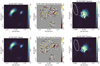 |
Fig. C.1. Highest-likelihood EPL lens models for alternative datasets. Each row illustrates a different assumption for the noise added to empty regions. From left to right: Model image, normalized residuals, and reconstructed source. Top row: Dataset where the modified image uses a σ10 dispersion. Bottom row: σ20 dispersion. Fluxes are in units of 10−18 erg s−1 cm−2. |
Appendix D: Strong gravitational lens around low-redshift galaxies
In Table D.1 we list strong gravitational lens systems associated with galaxies at z < 0.05 reported in the literature. Among these, the lensed source presented in this work is the most distant, and the system is only the second known case involving a spiral lens galaxy at such low redshifts.
Strong lensed systems by z < 0.05 galaxies.
All Tables
All Figures
|
Fig. 1. Right panel: Composite image of CGCG 012-070 obtained from the Pan-STARRS archive (Chambers et al. 2016), covering a region of 60 × 60 arcsec2. The image combines the r, i, and z bands. The green square indicates the NIRSpec field of view, which encompasses the inner region of the galaxy’s bulge. Small top panels: [O III] λ5007 (left) and Hα (center) flux maps for the z ∼ 2.89 lensed object, and a composite image (right), with the image of the lensed object shown in red and the 2.0 μm continuum image of the galaxy CGCG 012-070 in green. Bottom panel: Spectrum at the position of the lensed component A, identified in the top left panel. The observed spectrum is shown in black, the stellar population contribution of CGCG 012-070 in red, and the gas component in blue. The insets provide a zoom-in on the [O III] and Hα regions for the lensed object. The [Fe II] and H2 labels, identified in black, represent Fe and H2 lines from the foreground galaxy. |
| In the text | |
|
Fig. 2. Highest-likelihood EPL lens model. Each row illustrates a different emission line. From left to right, we present the modified (noise-added) observed image, the model image, the normalized residuals, and the reconstructed source. The top row details the [O III]λ5007 results, whereas the bottom row displays the Hα reconstruction, utilizing the mass model obtained from fitting the [O III]λ5007 emission. Fluxes are in units of 10−18 erg s cm−2. |
| In the text | |
|
Fig. A.1. CGCG 012-070 galaxy. Top left panel: 2.0μm continuum image of CGCG 012-070, obtained from the NIRSpec data cube. Other top panels: Flux distributions of the [Fe II]1.6440μm, Paα, and H22.1218 μm emission lines. Gray regions represent masked out areas where the S/N < 3 and regions outside the NIRSpec FoV. The cross marks the position of the continuum peak. Bottom panel: Observed spectrum (in black), integrated over a 0 |
| In the text | |
|
Fig. B.1. Integrated spectra for components B (top) and C (bottom). In each panel, the observed spectrum is shown in black, the stellar population contribution of CGCG 012-070 in red, and the gas component in blue. The insets provide a zoom-in on the [O III] and Hα regions for the lensed object. The [Fe II] and H2 labels identify emission lines from the foreground galaxy. |
| In the text | |
|
Fig. C.1. Highest-likelihood EPL lens models for alternative datasets. Each row illustrates a different assumption for the noise added to empty regions. From left to right: Model image, normalized residuals, and reconstructed source. Top row: Dataset where the modified image uses a σ10 dispersion. Bottom row: σ20 dispersion. Fluxes are in units of 10−18 erg s−1 cm−2. |
| In the text | |
Current usage metrics show cumulative count of Article Views (full-text article views including HTML views, PDF and ePub downloads, according to the available data) and Abstracts Views on Vision4Press platform.
Data correspond to usage on the plateform after 2015. The current usage metrics is available 48-96 hours after online publication and is updated daily on week days.
Initial download of the metrics may take a while.