| Issue |
A&A
Volume 702, October 2025
|
|
|---|---|---|
| Article Number | A76 | |
| Number of page(s) | 30 | |
| Section | Catalogs and data | |
| DOI | https://doi.org/10.1051/0004-6361/202449335 | |
| Published online | 09 October 2025 | |
Searching for substellar companion candidates with Gaia
I. Introducing the GaiaPMEX tool
1
LESIA, Observatoire de Paris, Université PSL, CNRS, Sorbonne Université, Université de Paris,
5 place Jules Janssen,
92195
Meudon,
France
2
Pixyl,
5 av du Grand Sablon
38700
La Tronche,
France
★ Corresponding author: This email address is being protected from spambots. You need JavaScript enabled to view it.
Received:
24
January
2024
Accepted:
3
September
2024
Abstract
Context. The Gaia mission is expected to yield the detection of several thousands of exoplanets, perhaps at least doubling the number of known exoplanets. However, only 72 candidates have been reported with the publication of the Gaia third data release, or third Gaia data release (GDR3). Although a greater harvest of exoplanets is expected to occur with the publication of the astrometric time series in the DR4 in 2026, the GDR3 is already a precious database that can be used to search for exoplanets beyond 1 au.
Aims. With this objective, we characterized multiple systems by exploiting two astrometric signatures derived from the GDR3 astrometric solution of bright sources with G<16. We have the proper motion anomaly, or PMa, for sources also observed with Hipparcos and the excess of residuals present in the renormalized unit weight error (ruwe) and the astrometric excess noise (AEN). These astrometric signatures give an accurate measurement of the astrometric motion of a source seen with Gaia, even in the presence of non-negligible calibration and measurement noises.
Methods. We introduce a tool called Gaia DR3 proper motion anomaly and astrometric noise excess, or GaiaPMEX for short, that is able for a given source to model the astrometric signatures that are hidden within the PMa, ruwe, and AEN by a photocenter orbit due to a companion with a certain mass and relative semi-major axis to the primary star (sma). GaiaPMEX calculates a confidence map of the possible companion’s mass and sma, given the actual measurements from GDR3, and Hipparcos, when available. This tool allowed us to determine for any source of interest if it may be a binary (or planetary) system and the possible companion’s mass and sma.
Results. We find that the astrometric signatures can allow for identification of stellar binaries and hint toward companions with a mass in the planetary domain. The constraints on mass are, as expected, degenerate, but when allowed, coupling the use of PMa and ruwe or AEN, they may significantly narrow the space of solutions.
Conclusions. Thanks to combining Gaia and Hipparcos, planets are expected to be most frequently found within 1–10 au from their star, at the scale of Earth-to-Saturn orbits. In this range of sma, exoplanets with a mass down to 0.1 MJ are more favorably detected around M-dwarfs closer than 10 pc to Earth. Some fraction, if not all, of companions identified with GaiaPMEX may be characterized in the future using the astrometric time series that will be published in the forthcoming DR4.
Key words: astronomical databases: miscellaneous / astrometry / planets and satellites: detection / binaries: general / brown dwarfs / planetary systems
© The Authors 2025
 Open Access article, published by EDP Sciences, under the terms of the Creative Commons Attribution License (https://creativecommons.org/licenses/by/4.0), which permits unrestricted use, distribution, and reproduction in any medium, provided the original work is properly cited.
This article is published in open access under the Subscribe to Open model. This email address is being protected from spambots. You need JavaScript enabled to view it. to support open access publication.
1 Introduction
Finding and characterizing exoplanets has become one of the most active areas in astronomy. So far, most exoplanets have been found by the transit and the radial velocity (RV1) techniques, as seen in the few publicly available exoplanet catalogs. Notably, Gaia absolute astrometry is expected to identify (tens of) thousands of new exoplanets and brown dwarfs (BD) in the near future (Perryman et al. 2014; Sahlmann et al. 2015; Holl et al. 2022; Gaia Collaboration 2023a; Holl et al. 2023).
The current number of exoplanet candidates identified with third Gaia data release (GDR3) astrometry (72; Gaia Collaboration 2023a) is still much below expectations. Therefore, a major challenge is to exploit the Gaia data currently made public in the online catalogs in its most recent data release (DR3; Gaia Collaboration 2021) to detect unknown exoplanet candidates, as nicely illustrated with the discovery of AF Lep b (Mesa et al. 2023; Franson et al. 2023; De Rosa et al. 2023). Incidentally, Gaia's astrometry can also help validate (or reject) candidate exoplanets detected by other means (RV, transit, imaging) and further characterize them (Kiefer et al. 2019, 2021; Kiefer 2019; Kervella et al. 2019, 2022; Brandt et al. 2019; Dalal et al. 2021; Brandt 2021; Feng et al. 2021, 2022; Xiao et al. 2023; Philipot et al. 2023b,a) or aid in assessing the existence of a companion (possibly supplementary) of a given star or set of stars of interest.
With this objective, we set up a tool called GaiaPMEX for Gaia DR3 proper motion anomaly and astrometric noise excess based on the original works of Kiefer et al. (2019); Kervella et al. (2019); Kiefer (2019); Kiefer et al. (2021); Kervella et al. (2022) that allows for determination of the mass of possible candidate companions and their relative semi-major axis in relation to their primary star (abbreviated to sma hereafter) from consideration of, individually or in combination, the constraints from the proper motion anomaly (hereafter PMa; Kervella et al. 2019; Brandt 2021; Kervella et al. 2022), the astrometric excess noise (AEN; see Kiefer et al. 2019; Kiefer 2019; Kiefer et al. 2021), and the renormalized unit weight error (ruwe; see Lindegren et al. 2018, 2021). This tool models, within a Bayesian framework, the observed AEN, ruwe, and PMa through simulated outcomes of Gaia's observations of a source if it had a companion of a given mass and sma. It leads to a 2D confidence map of the companion mass and sma. Introducing this tool is the purpose of the present paper; a series of further papers will report the results of its application on other systems.
In Sect. 2, we recall the definitions of AEN, ruwe, and PMa. In Sect. 3, we describe our reverse-engineering method to determine the noise levels of Gaia's observations of individual sources. In Sect. 4, we explain the modeling of any star’s orbital motion due to a companion and the simulations of Gaia astrometric measurements of that star. In Sect. 5.1 we define the PMa, ruwe, and AEN astrometric signatures. In Sect. 6, we present the GaiaPMEX tool in detail. In Sect. 8, we show illustrative examples of the application of GaiaPMEX on a few chosen sources. Finally, in Sect. 9, we discuss the perspectives opened by the application of this tool regarding the detection of exoplanets and brown dwarfs using Gaia.
2 Astrometric excess noise, RUWE, and proper motion anomaly
2.1 The astrometric excess noise
The AEN of a source, as introduced in Gaia Collaboration (2016), is the excess of scatter in the residuals of along scan angle measurements compared to the astrometric displacement of the source modeled as a single-star, that includes position, linear proper motion and parallactic motion. At each epoch of transit of a source along one of the detectors, there is a specific scan direction, the along scan direction (AL), along which the source image is moving during the rotation of the spacecraft. The position of the source on the detector can be determined in 2D, since there is also an across scan (or AC) direction, but it is much less precisely measured along the AC than along the AL direction. Therefore, in all Gaia data releases, only the AL angles are used as astrometric measurements to determine the main astrometric data of a source (Lindegren et al. 2016, 2018, 2021).
In the GDR3, as in previous releases, the process of fitting the astrometric data is iterative. At each iteration, individual errors, σAL, of AL angle measurements performed during a transit of a star on the detector are estimated or updated and then used to calculate a χ2. Since DR2 (Lindegren et al. 2018), a spacecraft attitude excess noise σatt is quadratically added to σAL in the calculation of the χ2. Its amplitude is typically about 0.076 mas, while individual measurement errors are within 0.05−0.15 mas (Lindegren et al. 2021). Both form a “formal error”  . We give more details and estimation of their variations with respect to the magnitude, color, right ascension (RA) and declination (Dec) of targets in Sect. 3.1. Their time series will only be known upon the publication of the DR4. The monitoring of the residuals root-mean-square shows that the measurement and excess attitude errors are constant most of the time, with rare deviations (see Fig. A.2 in Lindegren et al. 2021). We thus assume in the following that the attitude excess noise of a time series for any given target remains relatively constant in time. With this assumption, the χ2, as it appears in the archives (namely astrometric_chi2_al), written here
  is
is
 (1)
(1)
where Rℓ are the residuals of the N astrometric measurements (astrometric_n_good_obs_AL) after subtraction of the fitted model. If some additional calibration noise – that is, a non-subtracted residual instrumental jitter beyond the attitude excess noise – or real astrometric signal were to be present, it would not be accounted for in the formal errors used to calculate the χ2 and the reduced χ2 would be larger than 1. Deviations of the reduced χ2 beyond 1 are accounted for in the AEN (astrometric_excess_noise). To calculate the final uncertainties of fitted parameters of a given target, the AEN is quadratically added to the formal error of any astrometric measurements such as to impose a reduced χ2 of 1. Still assuming that the errors are uniform along the time series, the AEN is related to the residuals sum of square through
 (2)
(2)
counting N − 5 degree of freedom (DOF), with five parameters fit to the astrometry. The exact definition of the AEN involves possibly non-uniform errors and it is fixed iteratively during the reduction. Its value might thus slightly deviate from this definition. The level of the additional calibration noise still present in the data, not accounted for in the formal error of Eq. (1) but contributing to the AEN in Eq. (2), strongly depends on the magnitude and the color of the observed targets (Lindegren et al. 2016, 2018, 2021). We invented a method to estimate it for any source from the whole Gaia catalog of bright sources with magnitude G < 16, as thoroughly explained in Sect. 3.4.
The identification of many zero-valued AEN for sources dimmer than G=13 led us to become aware of an issue with the estimation of the calibration noise in the GDR3’s reduction. When the χ2 was smaller or equal to the 95 th-percentile of the χ2 distribution with NDOF degree of freedom, that is, when the reduced χ2 was smaller than  , the AEN was almost always fixed to zero in the archives (Lindegren et al. 2012). For sources dimmer than G=13, the attitude excess noise, common to all sources observed at the same epoch on the detector, overestimates the calibration noise and thus the format error to compute the χ2 (Lindegren, priv. comm.). This led to an AEN wrongly fixed to zero for many sources beyond G=13, thus erasing any information on supplementary signals. Below G=13 this problem did not arise, because the calibration noise was conversely underestimated by the attitude excess noise, leading always to strictly positive values of the AEN. Our present understanding is that the AEN can be used as a binarity indicator and even used to characterise orbital motion, as long as the calibration noise and the attitude excess noise are both well known, and that the zero-valued AEN are discarded. The renormalized unit weight error, discussed in the next section, being directly proportional to the reduced χ2 will be less problematic in this regard because it is not cut off below some value.
2.2 The renormalized unit weight error
An alternative to overcome the above issue is to use the renormalized unit weight error, or ruwe, instead of the AEN. By definition (Lindegren et al. 2018),
 (3)
(3)
where u0 is a factor that depends on magnitude and color. It can be determined from the GDR3 database values of  or astrometric_chi2_al), ruwe and number points N or astrometric_n_good_obs_al. With the approximate Eqs. (1) and (2), the ruwe and the AEN are directly associated:
 (4)
(4)
The ruwe is a unit-less scalar, but by the use of this formula, it could be conveniently transformed to an AEN. With a unit of angle – expressed in milli-arcsecond (mas) in the catalog – the AEN is directly commensurate to any possible astrometric motion – in au if divided by the parallax. A large value (>1.4) for a source is often accepted as indicating binarity. In many cases, this is indeed true, but it is nevertheless a misinterpretation of the DR3’s documentation, rather cautiously indicating that well-behaved sources (single or not), that is, for which the five-parameter fit gives a reasonably good fit, should have ruwe<1.4. We noticed, indeed, that the deviation of the ruwe above 1 in the GDR3 catalog is sometimes unreliable as a binarity indicator. This is most frequent for sources whose Gaia data were fit using six parameters (astrometric_params_solved=95). The case of the star β Pictoris is an excellent counter-example, with a ruwe of 3.07, that, we show in Sect. 8.5, can be explained by noise only, for this very bright star.
2.3 The proper motion anomaly
The PMa, as initially introduced in Kervella et al. (2019), is the proper motion offset between the Hipparcos-Gaia average proper motion (with a baseline ∼24.5 years), and the GDR3 fitted linear proper motion (with a baseline of 36 months). It thus measures an acceleration of the primary star due to the presence of a long-period secondary companion. The most recent measurements of PMa can be found in Kervella et al. (2022) as well as in Brandt (2021) with a different treatment of the global reference frames matching between GDR3 and the Hipparcos International celestial reference system (ICRS for short). In brief, noting μ the 2D proper motion, with index HG for “Hipparcos-Gaia",
 (5)
(5)
The non-linear perspective acceleration is assumed to be corrected in μHG. In this sense, μHG is the average 3-D Hipparcos-Gaia linear proper motion projected on the tangent plane at GDR3 epoch. Moreover, the effect of perspective acceleration is taken into account in the GDR3 astrometric solution, and μGDR3 is thus already the proper motion of the star in the Cartesian tangent plane. With these definitions, we can thus consider that μPMa is the projected tangential PMa as measured from a reference frame co-moving with the system’s barycenter.
As illustrated in Fig. 1, for any mass and sma, there always exists a longitude of ascending node Ω that fits any PMa position angle, the mass and sma can only be constrained from ‖PMa‖. When referring to PMa in the rest of the text, we thus always refer to ‖PMa‖, that is:
 (6)
(6)
Even though the PMa measures a variability in the proper motion of a star, noise in the astrometric measurement may induce a non-zero PMa. We assess the significance of the PMa in Sect. 5.2.2. It turns out that this is different than comparing the value of the PMa to its error bar that is calculated from the published measurement errors from Gaia and Hipparcos.
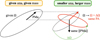 |
Fig. 1 Illustration of the equality of PMa modulo Ω between two systems with the same central star and a companion on a long-period orbit but with different values of sma and mass. For a given sma and a given mass of the companion (left panel) the PMa is directed toward the companion. There exists a smaller sma and a larger mass for which the ‖PMa‖ is the same (right panel) but the orientation at equal Ω is different. Nevertheless, it is possible to align the PMa on the same position angle (PA) by rotating the system by some ΔΩ. |
3 Noises and errors in Gaia observations
One the issues with interpreting correctly the AEN, ruwe and PMa as indicators of binarity and even measurements of companion’s properties, is our ignorance, a priori, of the noise budget in those quantities. Indeed, measurement noise and instrumental calibration noise participate at a certain degree in the excess of residuals beyond “formal error” (see Sect. 3.1 for a definition), as well as in any excess of proper motion fitted to noisy astrometric data. To complicate the task further, the level of those noises and error in Gaia data for any given source is not published and thus unknown to the community. As a prerequisite to the functioning of GaiaPMEX, whose goal is to model the astrometric motion beyond noise in AEN, ruwe and PMa, we thus present, in the following sections, a method that we developed to determine the noises and error levels in Gaia data for any source with G<16.
3.1 The formal error
What we call the formal error, σformal, is the unknown error that appears in the denominator of  in Eq. (1), that is,
  . Combining this equation with Eq. (2) led us to express a simple approximation of
  with respect to AEN:
 (7)
(7)
The formal error could thus be guessed by inverting this formula for all the sources observed in the GDR3 that have an AEN not compatible with 0 mas, that is, with an astrometric_excess_noise_sig ≥2 (Lindegren et al. 2012):
 (8)
(8)
This estimate of the typical errors used in the  for several million sources allowed us to study the impact of magnitude, color, RA and Dec on GDR3 astrometric errors, and, more specifically, as we show in Sects. 3.2 and 3.3 of the attitude excess noise and the AL measurement errors. We adopted the bins defined in Table 1. To adapt to more rapid variations of the errors between magnitudes of 10.5 and 13.5, we adopted a smaller bin size ∼0.1 between 10.5 and 12.5. Moreover, a strong discontinuity in the errors occurs at G=13. It is related to the change in window class (or WC) from G<13 (WC0) to G>13 (WC1). It goes with a different level of charge transfer inefficiency (CTI) that is increasing in WC0 up to G=13, but strongly decreasing in WC1 (Lindegren et al. 2021). Because of this, we had to adopt an even smaller bin size of 0.05 between 12.5 and 13.5 G-mag.
Bins used for G magnitude, Bp − Rp color, RA, and Dec.
In each magnitude-color or RA–Dec bin, we calculate the median formal error of all sources in these bins, respectively σformal (mag, color) and σformal (RA, Dec). This gives the relationship between formal error and magnitude & color or RA & Dec. Figure 2 shows the variations of the median formal error for the Gaia sources with AEN>0 mas and brighter than G=16, with respect to those parameters. We consider separately the sources whose data were fit by a five parameters model (astrometric_params_solved = 31), hereafter called ‘5p’ dataset, and those whose data – astrometry plus photometry – were fit by a six parameters model (astrometric_params_solved = 95) that includes an astrometric estimate of the effective wavenumber, or pseudocolor, veff, hereafter called ‘6p’ dataset. The sources whose data were only fit by a two-parameter model were not considered. Interestingly, this shows that the most crowded regions of the Galaxy have a larger error on average, as well as the sources with a G-mag of about 7–9. This latter dependence on magnitude agrees well with Fig. A.1 of Lindegren et al. (2021).
3.2 Attitude excess noise
The Gaia spacecraft attitude is modeled during the data reduction. It converts a rigid solid-body motion within the ICRS reference frame into Gaia's own reference frame where the CCDs are fixed (Lindegren et al. 2021). It thus models part of the path followed by any source along the detectors during a transit. This model suffers from time-dependent attitude excess noise, due, for example, to micro-clanks, calibration errors, etc., and has a typical level of 76 μ as on average (Lindegren et al. 2021). The attitude excess noise varies with time but at a given epoch all stars observed share a common attitude excess noise (Lindegren, priv. comm.). Depending on the magnitude and the color, σatt tends to over/under estimate the calibration noise (see also Sects. 2.1 and 3.4).
The time-dependency of formal errors or attitude excess noise is not available. We can only assume that for any source, those errors are relatively constant (see, e.g., the Fig. A.3 in Lindegren et al. 2021 for an example with time-dependent attitude excess noise variations). Nonetheless, for a given source with specific RA & Dec direction, the attitude excess noise is probed at more-or-less regularly spaced epochs because of the scanning law of the spacecraft. Sources in different directions might thus probe disjoint sets of attitude excess noise values, and the mean attitude excess noise might thus depend on the RA & Dec direction. Being fixed, by construction, for all stars observed at the same epoch, the attitude excess noise do not dependent on magnitude or color.
For any source in the GDR3 database that has AEN>0 mas, quadratically removing the AL measurement error from the formal error leads to the attitude excess noise. To do this computation, we need to know the AL measurement error for any source. By conversely quadratically subtracting the attitude excess noise from the formal error one in fact can estimate the AL measurement error. At any bin of magnitude & color, σformal (mag, color) is the median formal error among all sources in that bin, distributed on all directions of the sky. We thus expect that, at any magnitude & color, the median σatt is close to 76 μ as. This led to a first estimation of the AL measurement error, with respect to the magnitude and the color of the source, by applying
![Mathematical equation: $\sigma_{\mathrm{AL}}(\text{mag}, \text{color})=\sqrt{\left[\sigma_{\text{formal}}(\mathrm{mag}, \text{color})\right]^{2}-0.076^{2}}.$](/articles/aa/full_html/2025/10/aa49335-24/aa49335-24-eq17.png) (9)
(9)
This estimation is refined in Sect. 3.3. The AL measurement error of a given source depends mainly on the optical properties associated with a CCD measurement of its point spread function (PSF) on the detector, thus related to the magnitude and the color of the source. Linearly interpolating through this magnitude-color relationship, we can estimate the AL measurement error for any source of given magnitude and color (within available convex hull), or σAL, mc. Our best guess of the attitude excess noise for any source can then be obtained by quadratically subtracting this σAL, mc from the formal error:
 (10)
(10)
To allow for estimation of σatt even if a source’s AEN is compatible with 0 mas, and to smooth out scatter among sources with a similar sky location, we calculated a median attitude excess noise in every RA-Dec bins described in Table 1. Those median attitude excess noises are given in Table H.1. Figure 3 shows the dependence of the median σatt(RA, Dec) with the sky direction. It shows a strong dependence on this parameter, with more pronounced error, up to 0.13 mas, in crowded regions, such as the Magellanic clouds and the center of the Milky Way. For any given source, an estimation of the effective level of attitude excess noise is determined by linearly interpolating the RA-Dec relationship at the RA and Dec of the source. In the rest of the article, this interpolated value is called σatt.
3.3 Along-scan angle measurement error
Once σatt is estimated for any source given their RA-Dec direction, it is straightforward to determine the σAL for all the sources with AEN > 0 mas. We simply used
 (11)
(11)
As for σatt above, to allow for estimation of σAL, even if a source’s AEN is compatible with 0 mas and to smooth out scatter among sources with a similar magnitude and color, we calculated a median attitude excess noise in every magnitude–color bins are described in Table 1. The median AL measurement errors are given in Table H.2. It is available online with only an extract shown here at a Bp − Rp close to that of GJ 832, that is, Bp − Rp = 2.2. Figure 4 shows the dependence of the median σAL with the magnitude and color. For any given source, an estimation of the effective level of AL measurement error is determined by linearly interpolating the magnitude-color relationship at the G-mag and Bp − Rp color of the source. In the rest of the article, this interpolated value is called σAL.
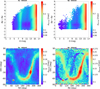 |
Fig. 2 Median formal error distribution σformal with respect to magnitude and color (top) and RA and Dec (bottom) in the GDR3 database of sources brigther than G=16. |
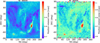 |
Fig. 3 Median attitude excess noise distribution with respect to RA and Dec in the GDR3 database of sources brighter than G=16. |
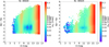 |
Fig. 4 Median AL measurement error distribution with respect to magnitude and color in the GDR3 database of sources brighter than G=16. |
3.4 Calibration noise
The level of the calibration noise truly present in the data depends mainly on the magnitude and the color of the observed sources (Lindegren et al. 2016, 2018, 2021). For any source, we calculated a normal model of the  , as thoroughly detailed in Appendix D. It accounts for the correlations between the co-adjacent astrometric AL angle measurements performed at the same epoch. The mean μχ2 of the distribution of the
  is related to σatt, σAL, and σcalib by
![Mathematical equation: $\mu_{\chi^{2}}=\frac{N_{A L}}{\sigma_{\mathrm{att}}^{2}+\sigma_{\mathrm{AL}}^{2}}\left[\left(N_{\mathrm{FoV}}-5\right) \sigma_{\mathrm{calib}}^{2}+N_{\mathrm{FoV}} \sigma_{\mathrm{AL}}^{2}\right]$](/articles/aa/full_html/2025/10/aa49335-24/aa49335-24-eq22.png) (12)
(12)
where NFoV is the number of field of view (FoV) transits on the detector, and NAL is the average number of AL angles collected per transit, that is, ≈int(N/NFoV). In the Gaia archives, the total number of AL angle measurements N is given by astrometric_n_good_obs_AL, while NFoV is given by astrometric_matched_transit. This equation leads to an expression of the σcalib for any source assumed single, that is,
 (13)
(13)
In any of the magnitude and color bins (Table 1), the best estimation of σcalib is thus that of single sources. The sources are separated into single and multiple stars, whose rate N (multiple)/N (sources) is unfortunately unknown. The distribution of σcalib in a given bin is thus the combination of both populations. According to Gaia's DR2 documentation2, rather than the median, one can more safely rely on the mode of the unit weight error (UWE) distribution3 to locate the median of single star’s distribution. Indeed, the mode is shown to be less affected by multiplicity than the median and is thus a better approximation of single star’s median. Conversely to what is adopted in the documentation, we have found that the 41st-percentile is not always a good approximation of the mode. We thus rather localized the mode in the σcalib distribution by iteratively excluding sources with a σcalib larger than twice 1.483 × MAD(σcalib) above the median, where MAD is the median absolute deviation. We then defined the mode as the median of this reduced distribution. We found that 3 iterations were necessary and enough to localise the mode. Figure E.1 shows this mode localization in the cumulative density functions of the σcalib distribution at some magnitude-color bins.
Figure 5 shows the distribution of σcalib with respect to G-magnitude and Bp − Rp color for the 5p and 6p datasets. The σcalib of the 6p dataset are systematically higher than the 5p dataset. This is an effect of the poorer-quality of the fit for those stars. For them, a large AEN or ruwe has to be interpreted with care. In both dataset, σcalib and magnitude are strongly correlated, especially for bright stars with G-mag <6, and to a lesser extent for early types with Bp − Rp<0.5 and late-types with Bp − Rp > 2.5.
4 Modeling of Gaia and Hipparcos astrometry
For later use, we define in this section our process for modeling Gaia and Hipparcos astrometric data. Our aim is to model the key data, namely PMa, AEN, and ruwe, which allow us to characterize the presence of companions and determine their main parameters, such as mass and sma. For any set of fixed companion, star and orbital parameters, we modeled by simulation the system’s photocenter orbit as if it was observed by Gaia or Hipparcos. In doing so, we accounted for instrumental and measurement noises in Gaia and Hipparcos data, and then performed a five-parameter fit of those datasets. We obtained residuals, as well as proper motion and centroid simulated measurements at GDR3 and Hipparcos epochs, respectively 2016.0 (Gaia Collaboration 2021) and 1991.25 (van Leeuwen 2007). We explain our method and the technical details of the simulations and the fit procedures in the following sections.
 |
Fig. 5 Maps of the calibration noise with respect to both G-mag and Bp − Rp color. Left: for the 5p dataset. Right: for the 6p dataset. |
4.1 Modeling photocenter orbits
The core of the orbit modeling is the same as the one used in the “Gaia astrometric noise simulation to derive orbital inclination” tool or GASTON for short (Kiefer et al. 2019, 2021). We always consider a 2-body system, with a primary A and a secondary B, possibly planetary, brown dwarf or stellar. We fix the reference frame of the orbit to be the system’s barycenter. With Keplerian parameters fixed for this system, we model the orbit of the photocenter of the system on the plane of the sky. The photocenter semi-major axis, aphot is determined from the total system’s semi-major axis, that is, the relative semi-major axis of the companion to the primary star; here written sma, through (Kiefer et al. 2021):
 (14)
(14)
with ϖ the parallax, β = q/(1 + q) the mass fraction, and B = L2/(L1 + L2) the luminosity fraction. The relative luminosity of the secondary over the primary is determined from semi-empirical mass-luminosity relation on the main sequence, at a typical age of 5 Gyr (see Kiefer et al. 2021 for more details). By default, we consider that the secondary may contribute to the photocenter’s position. Depending on the case at hand, one may instead consider a dark companion, whose luminosity is thus not contributing to the photocenter’s displacement. An illustration of the result of assuming instead a dark companion is shown in Sect. 8 for the case of α CMaB, that is, Sirius B, and whose companion Sirius A is resolved by Gaia and thus not contributing to α CMa B’s photocenter’s displacement.
The modeled orbits are then sampled at specific epochs, along specific directions, according to the scan law of Gaia and Hipparcos during their observation campaign. Noise is finally added to the individual measurements in a way that is specific to each instrument. This is further explained in the next Sects. 4.2 and 4.3.
4.2 Gaia DR3 sampling, scan-law, and noise
We sampled the modeled orbits at the GDR3 FoV-passage epochs and along the AL direction. The Gaia spacecraft is composed of two FoV, the ‘preceding’ and the ‘following’. They are separated around the spin axis of the spacecraft by a basic angle of 106.5∘ (Lindegren et al. 2012; see also Fig. 6). At a given epoch, the spin axis is moreover oriented in a certain direction conferring to the detector a certain orientation of its main axis, the AL axis, uAL. The law of the position angle (or PA) of uAL through time can be found in the GOST. Six to 9 astrometric measurements are performed at the same epoch during the transit of the source across the detector thanks to Gaia's spin, at a speed of 60′′/min (Lindegren et al. 2012).
The date of passage of a star on the Gaia detector and the PA of uAL can be predicted accurately using the Gaia observation forecast tool (GOST for short). However, this tool is only accessible online4. Instead, we built a code that performs the same predictions using the spacecraft scan law accessible from the commanded_scan_law database. As explained in Fig. 6, we calculate the angle between the direction of each detector (αd, δd) with the direction of the star at the GDR3 epoch (αs, δs). We used a gnomonic projection (see, e.g., Calabretta & Greisen 2002) to transform this angle into a vector on the plane of the detector. More specifically, there is a relationship between (η, ζ) the AL and AC coordinates on the detector, and the difference of coordinates between the pointing direction of the detector and the direction of the star. Moreover, given that the AL-direction is oriented at a PA=θAL, we found this relationship to be
 (15)
(15)
 (16)
(16)
Then we imposed that this vector should be contained within the used area of the detector. The zero origin of η and ζ is not located at the center of the detectors and is different in the two FoVs, as explained in (Lindegren et al. 2016). In terms of CCD (AL × AC) unit, compared to the center of the detectors, they are located at (−2.5,+0.5) for the preceding FoV and at (−2.5,−0.5) for the following FoV. The detectors have a common dimension of 0.66 × 0.74 degree2 with a grid of 9×7 CCDs. Dead zones are the wavefront sensor WFS2 (Gaia Collaboration 2016) and the area exterior to the detector. We assumed that CCD regions at less than a quarter of a CCD-sized distance to a dead zone is also a dead zone. This led to a better match of the number of predicted transits with the actual number of transits for any given star. We rejected a detection if the star fell on the dead zones. Figure 7 shows a representation of the detector and the geometry of the assumed dead zones, with GJ 832’s predicted average positions and AL scan direction orientations.
The time sampling of the scan law is ∼11 s. Therefore, during any transit of a source on the detector, several epochs are found, whereas only one epoch is required per transit. The spacecraft rotates at 1′′/s, and the largest of the diagonals of the detector have a dimension of 1∘. We thus determined, for any transit, the average epoch and average PA from all the predicted transit epochs found within a 1 hour window. We thus obtained for a given star all its theoretical epochs of transits through any of the two detectors with their corresponding PA of the AL direction. As a final step, we removed the epochs that fell at known gaps published in the GDR3 catalog5. The position of GJ 832 on the detector and the PA of the scan directions during its transits as retrieved from the scan-law is shown in Fig. 7.
We verified that the retrieved FoV transits matched those predicted by the GOST. Moreover their number are always close to those given by the astrometric_matched_transit in the GDR3 catalog. We noted that our calculation, consistently with the GOST, sometimes overestimated the number of actual FoV transits retained to calculate the astrometric solution in the GDR3. This happens most often to bright stars, thus indicating an effect of saturation that led to removal of some of the transits in the solution. In those cases, we randomly selected the correct number of epochs effectively used by Gaia in the GDR3 among all retrieved epochs of FoV passages.
We then assumed that the Gaia's AL measurements along the AL direction are distributed according to a normal law with as standard deviation, the noise σAL determined by the G and Bp − Rp of the source in consideration (see Sect. 3.3). Adding to this error, we added an epoch-specific offset randomly drawn from a normal distribution with standard deviation σcalib, determined with respect to the G and Bp − Rp of the source (see Sect. 3.4). One such simulation is shown in Fig. 8.
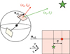 |
Fig. 6 Schematic representation of the orientation of one of Gaia's detectors (red arrow) compared to a star’s direction (green arrow). The solid circle represents the celestial sphere as seen from the Gaia center of mass, and the dashed-line circle represents the celestial equator. The two quadrilaterals represent Gaia's preceding (light red) and following (light yellow) FoV detectors. On the bottom right, we show the possible location of the star on the detector and the η angle that is measured projected along the AL axis (uAL). Arbitrary north and east directions are shown with the definition of the PA of the AL direction. They are not intended to exactly correspond to the top-left drawing but allowed us to define θAL, the eastward-oriented angle between uAL and the north. |
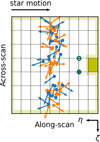 |
Fig. 7 Transits through the detector found for GJ 832 on the preceding FoV (blue) and the following FoV (orange). Each rectangle is a CCD, and the grid is 9×7. The cyan-filled black symbols represent the FoV origins, with a ‘+’ for the preceding and a ‘−’ for the following FoV. The black arrow at the top shows the direction of the source motion through the FoV. The dots show the average positions of the star on the detector at different epochs. The arrow connected to the dot indicates the average north direction at that epoch. The yellow regions depict the assumed dead zones, with the darker rectangle corresponding to the WFS2. |
4.3 Hipparcos sampled epochs
The Hipparcos-2 intermediate astrometric data (IADs; van Leeuwen 2007) are necessary to model the PMa as determined by Kervella et al. (2022). We here only focus on the PMa between GDR3 and HG baselines. The location of the centroid of the Hipparcos-2 data in the source barycenter reference frame has to be determined for any modeled orbit to find the HG average proper motion between epochs 1991.25 and 2016.0. In the Hipparcos-2 database the published source centroid is located along the fitted solution. This is not adequate for us because Hipparcos-2 used, when possible, more elaborate models including acceleration or orbital motion. However, Kervella et al. (2022) only considers the result of a five-parameter fit of the Hipparcos-2 IADs to derive the Hipparcos-2 proper motion and the location of the Hipparcos-2 source centroid at epoch 1991.25.
Therefore, for any source also observed with Hipparcos, we downloaded the IADs residuals from the Hipparcos-2 Interactive Data Access Tool6. These data include the orbit number (IORB), the epoch, the cosine and sine of the Hipparcos scan angle (related to the Gaia scan angle convention by ψ=θAL-π/2; Brandt 2021), the residuals of the fitted model (RES) and the formal errors (SRES).
We removed the data with negative or zero SRES that are rejected observations. To model Hipparcos observations of the astrometric displacement of the photocenter due to an orbital motion, we only need the part of the residuals at each IORB that cannot be due to supplementary non-modeled displacement. We thus calculated corrected residuals (CRES) by removing the local average from common IORB residuals. Then when simulating an orbit, those CRES are added along the Hipparcos scan direction.
Besides, to have an estimation of the typical dispersion associated with a source centroid position, we also calculated the Hipparcos-2 positional error for the considered source from the RA and Dec positional error published in the Hipparcos-2 catalog:
 (17)
(17)
An illustration of the Hipparcos data modeled for an arbitrary orbit is shown in Fig. 8.
 |
Fig. 8 Simulation of an orbital motion as seen by Hipparcos (red dots) and Gaia (DR3; blue dots) around GJ 832 for a companion mass of 100 MJ and sma=1 au, e=0, Ic=0∘. For visualization, we added a virtual proper motion of 30 mas/yr along the RA direction. The individual astrometric measurements are scattered along the along-scan directions at each FoV transit epoch with σAL=0.095 mas and σcalib=0.15 mas for Gaia and an average dispersion of ∼4.2 mas for Hipparcos. The orange and cyan crosses respectively mark the position of the fit centroid on the Hipparcos and Gaia datasets. |
4.4 Gaia and Hipparcos five-parameter model fit
For each modeled orbit, we applied a five-parameter7 fit to Hipparcos-2 and GDR3 simulated data. It included the RA-Dec centroid of data points, the linear proper motions μα and μδ, and the parallax ϖ. Given that we placed ourselves in the barycenter reference frame of the considered system, we thus fit the excesses of (positive or negative) offset, proper motion, and parallax only due to the presence of an orbital motion. Because of the orbital motion, the parallax measured in GDR3 deviates from the true value. Assuming that the current orbit was the true one, we first estimated the parallax error Δ ϖ from the fitted parallax excess in a first simulation. We then performed a second simulation, correcting the parallax by ϖ → ϖ − Δϖ. The 2D-fitted linear model is
 (18)
(18)
where the δμ are proper motion in α=RA cos Dec and δ=Dec tangent plane directions, Π(t) is the parallax ellipse depending on the coordinate of the star, and t0 the Hipparcos-2 or GDR3 epochs, respectively 1991.25 and 2016.0. We note that the effect of perspective acceleration (see, e.g., Michalik et al. 2014; Halbwachs et al. 2023) that mainly affect high proper motion targets close to Sun, is already corrected in the GDR3, so being a second-order effect we can ignore it here (Lindegren et al. 2021). To compare this linear model to the Hipparocs and Gaia measurements, we needed to project this model onto the along-scan directions, with position angle θAL, determined at the sampled epochs along the orbit:
 (19)
(19)
We separated components along Dec (north) and RA (east) directions. We subtracted this five-parameter model from the simulated data and calculate the residuals. For Gaia, they are further used in comparison to the tabulated AEN or ruwe published in the GDR3 catalog as explained in Sects. 5.1 and 6.
To calculate the PMa, the fit GDR3 proper motion, δμGDR3, was combined with the average proper motion between the fit positions of the photocenter at the Hipparcos-2 reference epoch and the GDR3 reference epoch, δμHG, through
 (20)
(20)
 (21)
(21)
This modeled PMa is compared to the PMa published in Kervella et al. (2022), as explained in Sects. 5.1 and 6.
5 The non-singleness of stars observed with Gaia
5.1 Astrometric signatures
To assess the non-singleness of stars from AEN, ruwe, and PMa, we defined (and introduce here) the “astrometric signatures”, further written as α. They properly quantify the deviation of AEN, ruwe and PMa beyond the level that they must have had if the sources were single.
5.1.1 The residuals astrometric signature
We first introduced the residuals unbiased estimator of variance a posteriori (UEVA) related to the  by
by
 (22)
(22)
This quantity’s square root, also known as regression standard error (RSE), is an unbiased estimator of the data typical error in the considered sample of measurements. The UEVA of any source, considering Eqs. (3), (7) and (22), can be estimated in two different ways, either using the AEN or the ruwe:
 (23)
(23)
 (24)
(24)
We consider both in the rest of the study. The UEVA of a single source (UEVAsingle) only accounts for calibration noise and AL astrometric noise. The distribution of UEVAsingle is obtained from the normal model of the χ2 distribution of the residuals, determined in Appendix D, Eqs. (D.8) and (D.9). It led to a normal distribution  (μUEVA,single, σUEVA,single) of the UEVAsingle with
![Mathematical equation: $\mu_{\mathrm{UEVA}, \text{single}}= \frac{N_{A L}}{N_{A L} N_{\mathrm{FoV}}-5}\left[\left(N_{\mathrm{FoV}}-5\right) \sigma_{\text{calib}}^{2}+N_{\mathrm{FoV}} \sigma_{\mathrm{AL}}^{2}\right]$](/articles/aa/full_html/2025/10/aa49335-24/aa49335-24-eq37.png) (25)
(25)
![Mathematical equation: $\begin{align*} \sigma_{\mathrm{UEVA}, \text{single}}^{2}= & \frac{2 N_{A L}}{\left(N_{A L} N_{\mathrm{FoV}}-5\right)^{2}}\left[N_{A L}\left(N_{\mathrm{FoV}}-5\right) \sigma_{\text{calib}}^{4}\right. \\ & \left.+N_{\mathrm{FoV}} \sigma_{\mathrm{AL}}^{4}+2 N_{\mathrm{FoV}} \sigma_{\mathrm{AL}}^{2} \sigma_{\text{calib}}^{2}\right]. \end{align*}$](/articles/aa/full_html/2025/10/aa49335-24/aa49335-24-eq38.png) (26)
(26)
Ingredients needed to calculate μUEVA,single and σUEVA,single for any source are thus G-mag, Bp − Rp, RA and Dec to estimate the noises; and NFoV, as well as NAL=int(N/NFoV). The variation of the single-star RSE with respect to magnitude is compared to the level of σAL in Fig. 9. It compares well and agrees with the same curves plotted in Fig. A.1 in Lindegren et al. (2021) determined directly from the unpublished time series and images. This shows that our estimation of UEVAsingle in Eq. (25) provides a reliable estimation of the ground level of the UEVA for any source.
For a non-single star, when adding the orbital motion, the UEVA may positively deviate from UEVAsingle. We define the residuals astrometric signature as the angular excess that has to be quadratically added to the ground level UEVAsingle to recover the UEVA of the residuals of the given source. It thus measures, in units of milli-arcseconds, the strength of non-singleness of the source. It is written αUEVA and is formally defined as
 (27)
(27)
Using μUEVA,single as the expectation value of UEVAsingle and the AEN (Eq. (23)) or the ruwe (Eq. (24)) to estimate UEVA, we can determine αUEVA for any source. For a single star, as further developed in Sect. 5.2, because of the diverse astrometric noises that depends on the star’s magnitude, color and sky coordinates, the UEVA follows a broadened distribution that extends around UEVAsingle. It leads to αUEVA=0 if the UEVA is smaller or equal to UEVAsingle and positive values otherwise. For non-single sources, αUEVA may become strongly positive if the astrometric motion dominates over the astrometric noises. In that sense, αUEVA is indeed an astrometric signature.
Figure 10 compares the αUEVA calculated from UEVAaen or UEVAruwe to respectively AEN or ruwe for both 5p and 6p datasets. It shows that the αUEVA is almost equal to AEN beyond AEN=2 mas. The AEN could thus be directly interpreted as an astrometric signature in this regime. While there is a clear linear correspondance between ruwe and αUEVA beyond ruwe=1.4, with an approximative slope of ∼0.2, the thickness of the relation makes a direct astrometric interpretation more difficult. This is worse for the 6p dataset where the range of possible αUEVA for a given ruwe is even more spread out, due to the larger levels of noise compared to the 5p dataset. Irrespective of the dataset, below AEN=2 mas and ruwe=1.4 the range of possible αUEVA is significantly broader. Some values are as low as 10 μ as, thus dominated by noise and insignificant.
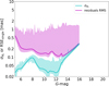 |
Fig. 9 Along-scan astrometric measurement precision variations with respect to G-mag for all GDR3 sources. The magnitude interval is enlarged up to G=20 for direct comparison to Fig. A.1 in Lindegren et al. (2021). The cyan line shows the median σAL, and the magenta line shows the median RSEsingle. Colored regions show the extent of σAL and RSEsingle with respect to color at each magnitude. |
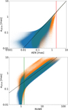 |
Fig. 10 Astrometric signature αUEVA calculated from either AEN (top) or ruwe (bottom) and compared to the quantities in the 5p (blue dots) and 6p (orange dots) datasets. The dashed black line shows, respectively, the αUEVA=AEN and αUEVA=0.2 ruwe relationships mentioned in the text, through Eqs. (23), (24) and (27). The red and green vertical lines show, respectively, the AEN=2 mas and ruwe=1.4 thresholds. |
5.1.2 The PMa’s astrometric signature
Similar to αUEVA, a PMa’s astrometric signature can determine the excess that has to be quadratically added to PMasingle to recover the PMa of the given source measured in Kervella et al. (2022). Indeed, for a given orbit, the PMa should be given by a constant vector (c), that is, the “noiseless” orbital contribution, plus a stochastic vector (ξ), that is, the pure noise contribution. The expectation value of the square-norm of the PMa is thus
 (28)
(28)
since 〈ξ〉=0 and c is constant. The first term is the pure orbital contribution to the PMa, null if there are no orbital motion, that is, the astrometric signature that we seek. The second rightmost term is the squared-norm of PMa for a single star, or  . Therefore, we introduce αPMa the PMa’s astrometric signature, formally defined as
 (29)
(29)
It is theoretically possible to determine the typical level of PMasingle. However, conversely to the UEVA, there are no theoretical formula for estimating this distribution. We thus needed to perform simulations to estimate its mean and standard deviation, depending on the RA, Dec, Bp-Rp and G of the sources. We determined the typical distribution followed by PMasingle in Sect. 5.2.2.
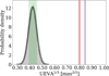 |
Fig. 11 Distribution of UEVA1/3 expected for a single star applied on the case of HD 114762. The green area shows the region spanned by the median plus or minus the standard deviation. The UEVA1/3 estimates from the AEN and ruwe published in the GDR3 archive are shown in red and purple, respectively. The thick black line shows the normal model derived from Eqs. (25) and (26). All values of noises used in the models are given in Table B.1. |
5.2 The significance of the astrometric signatures
5.2.1 Significance of αUEVA
As introduced in Sect. 5.1.1, the UEVAsingle could be modeled by a normal distribution  (μUEVA,single, σUEVA,single) whose parameters are written in Eqs. (25) and (26). Rigorously speaking, as explained in Appendix D, the UEVAsingle is a linear combination of χ2 and normal distributions, with the main terms distributed according to the χ2 law. Under the prescription of Wilson & Hilferty (1931) (see also Canal 2005), the cubic-root of the UEVA more closely resembles a normal distribution. We thus used UEVA1/3 and assumed that it followed a normal distribution
  (μ1/3, σ1/3). We approximated its parameters by μ1/3=μ1/3 and σ1/3=σμ−2/3/3 by applying error propagation. Figure 11 shows the resulting distribution of 100 000 simulations of UEVA1/3 obtained when assuming that a source – here, for example, HD 114762 – is a single star, and compares it to the normal model.
The significance of αUEVA naturally corresponds to the p-value of the UEVA1/3 as calculated from either the AEN or the ruwe from the GDR3, within the  (μ1/3, σ1/3) single-star distribution. This p-value is converted to an N−σ significance, following the “normal law” relationship between the 1−2−3-σ levels and the 31.6−4.6−0.27% p-values. We defined that αUEVA is significant at Nσ−σ if
  > chi2.ppf(xNσ/100,NFoV−5) where chi2.ppf is the function of the python’s scipy.stats-module, and xNσ corresponds to the usual percentage at Nσ−σ (N=1: xNσ=68.3%; N=2: xNσ=95.4%; N=3: xNσ=99.73%). An αUEVA significant at 2−σ would thus imply that the AEN or ruwe would have a less than 4.6% chance to occur if the star was single.
We showed in Fig. 12 the distribution of αUEVA among all datasets. Its full range goes from about 0.1 μ as to 10 mas, but the αUEVA with a significance >2−σ rather span the range that is beyond 10 μ as.
The sample with an αUEVA significance larger than 2−σ contains 19.1 × 10⁶ sources, that is, about 25% of the sample of 75.9 × 10⁶ Gaia sources with G<16 and ϖ>0. Close to 9% of the sources (6.7 × 10⁶) have a significance larger than8 8−σ. Figure 13 shows d fdetec(Nσ) the number of detections per bin of (Nσ, Nσ + dNσ)–σ significance. They are compared to the theoretical distribution for only single stars, that is, d fsingle=Nsingle × exp  dNσ/
dNσ/  . The number of single stars, Nsingle, is determined with respect to an assumed binary (and multiple) rate in the sample, Γb=Nbinary/Nsample, using Nsingle=(1−Γb) × Nsample. Assuming a Γb of 0% (blue curve in Fig. 13), the single star distribution cannot explain the rate of detections beyond 1.5−σ. Moreover, since many systems must be non-single, considering 100% of single-stars in the sample obviously overestimates the number of detection below 1.5−σ. A more realistic value for Γb can be found by assuming that all the sources at 0−σ significance must be single. We then fixed Nsingle in such a way that dfsingle(Nσ=0) matches dfdetec(Nσ=0). As illustrated with an orange line in Fig. 13, we found a single-star rate of 47% and thus a Γb of 53% in this sample of sources brighter than G=16. The pollution from false-positives (FP) clearly equates/dominates over true positives below 2−σ. Beyond 2−σ, with a single-star rate of conservatively 47−100%, we estimate that about 9−19% of the selected binary or planetary systems could be single-star false positives. Thus, more than 80% of the selected sample beyond 2−σ significance are bona-fide binary, multiple or planetary systems. Beyond 3−σ the sample reaches 16% of the 76 millions sources, leading to single-star false positives rate of 0.9−2%. Thus, virtually all >3− σ sources are true binary, multiple or planetary systems, but about 14−24% of the non-single star sample is lost compared to using the 2−σ threshold. In the perspective of identifying binary, multiple or planetary systems candidates, we thus recommend, and adopt, that an αUEVA, whose significance is above the 2σ level, has to be considered as a strong candidate, with a 9−19% chance that it actually is a single-star FP.
We use HD 114762 as an illustration for the significance of astrometric signature. This system was known for a long time for hosting a candidate planet HD 114762 b with an m sin i of 11 MJ (Latham et al. 1989; Kane et al. 2011). Confirming suspicion (Cochran et al. 1991; Hale 1995; Halbwachs et al. 2000), it was further shown using the astrometry from Gaia DR1, then GDR3, that HD 114762 b was actually an M–dwarf (Kiefer et al. 2019; Winn 2022; Gaia Collaboration 2023a). This was first shown using the significant value of AEN of 1.09 mas (Kiefer et al. 2019); then a proper astrometric orbit solution was obtained using the private GDR3 timeseries (Gaia Collaboration 2023a). In the light of the new framework introduced above, we found indeed that its GDR3 residuals astrometric signature rejected the single star hypothesis.
If HD 114762 was a single star – or orbited by an undetectable companion – the Gaia measurements would lead to AENsingle=0.251 ± 0.035 mas, ruwesingle=1.11 ± 0.13, and UEVAsingle=0.076 ± 0.018 mas2. In comparison, using the values of AEN=0.708 mas and ruwe=3.16 found in the GDR3 for HD 114762, we determined that UEVAaen=0.514 mas2 and UEVAruwe=0.607 mas2. The astrometric signature deduced in both cases by applying Eq. (27) are αastro,aen=0.662 mas and αastro,ruwe=0.729 mas. The p-value of  and
and  in the distribution of
  corresponds to a significance >9−σ (see Fig. 11). A single star may explain the AEN and the ruwe in close to 0% of the simulations. Both the AEN and the ruwe thus indicate the presence of a companion around HD 114762.
Assuming that the 84-day companion is responsible for this astrometric signature and that the star’s semi-major axis a*∼αUEVA/ϖ with the parallax ϖ=26 mas, and crudely applying Mc=a*(M*/M⊙)2/3(P/year)−2/3 with M*=1.05 M⊙ (Winn 2022), we find a possible mass of the companion of 86 MJ. The mass obtained is indeed much larger than 11 MJ but is less than its most recent estimation ∼ 0.3 M⊙ (Winn 2022). This just shows that αUEVA is not a measure of a*, leading us to develop a more sophisticated framework for interpreting αUEVA and infer main parameters of companions, as explained in Sect. 6.
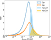 |
Fig. 12 Probability density functions of the astrometric signature in the 5p (blue line) and 6p (orange line) datasets. The colored histograms show the distribution of αUEVA whose significance is greater than 2σ, respectively blue and golden for the 5p and 6p datasets. |
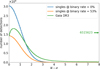 |
Fig. 13 Number of detections per bin of significance among the 76 million sources (green line) compared to the expected numbers for single stars if the global binary rate among all GDR3 sources is 0% (blue line) and 53% (orange line). The rightward arrow shows the number of sources with significance levels greater than greater than 8 σ. |
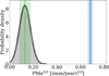 |
Fig. 14 Distribution of PMa2/3 generated from noise only for the case of GJ 832. The caption is the same as in Fig. 14. Here, the blue line and blue region show the PMa (at power 2/3) and its uncertainty taken from Kervella et al. (2022). The thick black line shows the normal model derived from the simulations themselves (see text for explanation). |
5.2.2 Significance of αPMa
The significance of αPMa corresponds to the p-value of the PMa2/3 within the distribution of  . This p-value is converted to an N−σ significance (see Sect. 5.2 for more details). As mentioned in Sect. 5.1.2, the distribution of
  is not known a priori because it strongly depends on the time sampling of the astrometric observations further fitted by a five-parameter model to measure the GDR3 proper motion, as well as the HG relative positions. Conversely to αUEVA, determining the distributions of αPMa thus requires performing many simulations of a single star observations given the main parameters, scan law, and noises of the given source.
We used the system of GJ 832 to illustrate the significance of PMa beyond the single star hypothesis. GJ 832 is an M0V star at a distance of 5pc and with a mass of 0.48 ± 0.05 M⊙. Its planetary system was discovered by Bailey et al. (2009), reporting one Jupiter-like planet with a period of 3416 ± 131 days and minimum mass of 0.64 ± 0.06 MJ. A second Earth-like planet was proposed for detection (Wittenmyer et al. 2014) but finally identified as a stellar activity artifact (Gorrini et al. 2022). The sma and minimum mass of GJ 832 b were further updated to 3.6 ± 0.4 au and minimum mass of 0.74 ± 0.06 MJ (Gorrini et al. 2022). This system is illustrative for us because it harbors one of the smallest mass planets leading to significant astrometric acceleration detected by combining Hipparcos and Gaia, and astrometric excess noise in the GDR3.
Figure 14 shows the PMa2/3 distribution obtained for GJ 832 in the hypothesis that it is a single star. We used the values of noises, including the Hipparcos position error, that are given in Table B.1. It leads to PMasingle=0.060 ± 0.032 mas yr−1 and  =0.153 ± 0.054 (mas yr−1)2/3, while Kervella et al. (2022) measures PMa=0.565 ± 0.027 mas yr−1, and equivalently PMa2/3=0.683 ± 0.022(mas yr−1)2/3. If comparing to a zero-point PMa offset of zero, that is, when neglecting noise, the PMa2/3 would have an apparent signal-to-noise ratio (S/N) of 30. But the distribution of
  , because of noise, strongly departs from zero as shown in Fig. 14. It leads to rather consider a positive zero-point offset and a larger error, that imply a more modest S/N of 10 for the PMa of GJ 832. We thus stress that the noise brings a major contribution to the zero-point offsets and errors that are used to determinate the S/N. For GJ 832, the p-value of PMa2/3 in the distribution of
  , implies a significance of the PMa >9−σ (see Fig. 14). Thus, it firmly indicates the presence of a companion in this system.
Distribution of parameters sampled at each tested bin of the mass-sma grid.
Since the orbital period of GJ 832 b is ∼6 yr, that is, smaller than the Gaia-Hipparcos baseline of 24.5 years, we would tend to crudely interpret the PMa here as the average orbital speed during GDR3 observations. Assuming thus that PMa/ , it leads to estimate the mass of GJ 832 b at 3.6 au to Mc ∼ 0.1 MJ. This mass is on the order of magnitude of the expected mass, though underestimated. The tool that we developed in Sect. 6 allowed us also to properly infer the main parameters of companions from the knowledge of PMa.
6 The GaiaPMEX method
We aim at calculating the confidence regions of possible mass and sma of a companion, for a Gaia source with a given αUEVA – either determined from AEN or ruwe – and/or αPMa. To do so, rather than using a Markov-chains Monte-Carlo approach, which is time consuming, we perform a mass-sma grid search within a Bayesian framework. At each node of the mass-sma grid, as summarized in Fig. 15, the values determined in the GDR3 and in Hipparcos-Gaia-(E)DR3 studies (Brandt 2021; Kervella et al. 2022) are compared to modeled PMa and UEVA (see Sect. 4). We defined a likelihood function in Sect. 6.3.1. The adopted Bayesian framework is explained in Sect. 6.3.2 and summarized in Fig. 16.
6.1 A uniform grid of log Mc and log sma
To probe different orders of magnitudes for the mass and sma, we define a uniform 2D-grid on log Mc and log sma with log-scaled Δ mass and Δ sma, as sketched in Fig. 15. In each bin, we draw log Mc and log sma within a uniform distribution bounded by the bin edges. We also draw Keplerian parameters of the possible companion orbits, namely e the eccentricity, ω the periastron longitude, Ω the longitude of ascending node, ϕ the phase, and Ic the orbit inclination, following the distributions summarized in Table 2. Parallax, ϖ, and stellar mass, M*, are drawn from normal distribution defined by prior knowledge on those parameters. The parallax is taken from the GDR3 catalog. By default, if M* is not given as input, it is first searched in the GDR3 Coordination unit 8 (CU8) catalog (Gaia Collaboration 2023b). We specifically looked for the final luminosity age and mass estimate (or FLAME) available for more than 140 millions sources with M*>0.5 M⊙, the mass-Flame that is determined from combining photometry, parallax and stellar models. Complying with studies of stellar masses reported in Gaia Collaboration (2023a) and Babusiaux et al. (2023), as well as the recommendations in the Gaia documentation9 and more specifically the “astrophysical parameters” section10, the uncertainty on the mass is assumed ∼ 10% if M*>0.7 M⊙ and 0.1 M⊙ if the mass is <0.7 M⊙. If the star is a giant we only use the CU8 stellar mass if it is within 1−2 M⊙, and we assume a 30%-uncertainty. If missing in this catalog, the stellar mass is instead estimated from the two first letter and digit of the spectral type given in the SIMBAD database11 assuming that the star is on the main sequence.
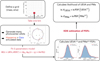 |
Fig. 15 Summary sketch of the analysis performed on one single bin of the grid. |
6.2 Modeling of PMa and UEVA
In each bin of the (mass, sma)-grid, we modeled by simulation many Gaia observations of photocenter orbits, due to the reflex motion of the source due to a companion at given mass – or log (mass) – and sma – or log (sma).12 For each modeled observation, we added noise in Gaia data (see Sects. 2.1 and 3.1), and then performed a five-parameter fit. Technical details on this modeling by simulation are explained in Sect. 4.1. Each simulation leaded to a value of PMa and a value of UEVA.
For each bin of the mass-sma grid drawn in Sect. 6.1, the full set of simulations obtained at a given (log Mc, log sma)-bin leaded to distributions of possible UEVA and PMa that would be measured in the GDR3 if the companion had such a mass and sma. We found that at least 100 simulations per bin are necessary to lead to a fine quality map. Running 300 simulations per bin performed better, leading to cleaner noiseless maps, with a computation time that was still tractable, though 3 × longer13. The maps that are shown here were obtained with 100 simulations per bin.
6.3 A Bayesian scheme for the 2D posterior distribution
From the modeled distributions, we determined a likelihood of the actual values of UEVA – either determined from AEN or ruwe – and PMa given the (mass,sma)n-model  = p(PMa, UEVA∣massn, sman). It is derived in Sect. 6.3.1 below. This likelihood was further used for a Bayesian inversion to determine the posterior distributions on mass and sma of the hypothetical companion, as explained in Sect. 6.3.2.
6.3.1 A log-likelihood of PMa and UEVA
One of the important issues met when defining a log-likelihood for PMa and UEVA, was to determine their probability density function (PDF) with ln  =ln PDF (data). They typically do not follow a normal-law, since both quantities are always positive. We show in Sect. 5.1 that, because the PDF of the squares PMa2 and UEVA are similar to χ2-distributions, their transformations to PMa2/3 and UEVA1/3 follow close-to-normal laws (Wilson & Hilferty 1931; Canal 2005). This ensured that our data distributions had PDF that were more compact and symmetrical as shown in Fig. 17.
Figure 17 illustrates the typical differences in the distributions of UEVA and UEVA1/3 as well as PMa, PMa2 and PMa2/3, for the case of a hypothetical 100−MJ companion at 1 au around GJ 832. Figure 18 also shows the difference in the KS-test of the normal law with the distributions of UEVA or PMa and respectively those of UEVA1/3 or PMa2/3 modeled at different values of sma. Generally for most sma from 0.5 to 100 au, the X1/3−transformation is a closer match to the normal law than simply UEVA or PMa. We thus adopt using UEVA1/3 and PMa2/3 for calculating the likelihoods.
For any (mass,sma)-bin of the grid, a Gaussian kernel density estimation (with the gaussian_KDE library from scipy) was performed on the distributions of the modeled UEVA1/3 and PMa2/3. This gives a good approximation of the true PDF of those quantities, as long as the sampling is dense enough, which is why we preferred using distributions that are not too extended and long-tailed. They can be used to derive the log-likelihoods as:
![Mathematical equation: $\begin{align*} \ln \mathcal{L}_{\mathrm{UEVA}} & =\ln \left[\mathrm{PDF}_{\mathrm{UEVA}^{1 / 3}}\left(\mathrm{UEVA}_{\mathtt{ruwe}}^{1 / 3}\right)\right] \\ \ln \mathcal{L}_{\mathrm{PMa}} & =\ln \left[\mathrm{PDF}_{\mathrm{PMa}^{2 / 3}}\left(\mathrm{PMa}_{\mathrm{HG}}^{2 / 3}\right)\right].\end{align*}$](/articles/aa/full_html/2025/10/aa49335-24/aa49335-24-eq62.png) (30)
(30)
Those log-likelihood give the probability of the data given a certain (mass,sma)-companion model and distributions of other Keplerian parameters. They are then used in GaiaPMEX in the inversion of the Bayesian formula to obtain the probability of the models given the data, and confidence regions on mass and sma, as explained in Sect. 6.3.2.
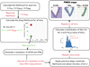 |
Fig. 16 Summary sketch of the Bayesian analysis performed on all bins of the grid to recover the posterior probability function on mass and sma. |
6.3.2 Bayesian inversion
Every bin n of the grid has thus a likelihood  and a corresponding log-likelihood
  . The bin nmax at which
  is maximized, reaching
  , is the (mass,sma)-model for which the data are best matching the UEVA and PMa distribution. At any other bin, we measured a likelihood ratio (LR) through
  .
.
To derive a probability function for mass and sma, we needed to determine at each bin n, what is the p-value of  . This is summarized in Fig. 16. In the ideal case of the likelihood-ratio test of some null hypothesis, the Wilks theorem states that with a large number of data,
  should follow a χ2 distribution with k degrees of freedom (Wilks 1938; Silvey 1970); k being the difference between the maximum number of degree of freedom (DOFmax=Ndata−Nparam), and the number of degree of freedom in the region constrained by the null-hypothesis where some of the parameters are fixed (DOFnull=Ndata−Nparam,unfixed). Here, fixing the only 2 parameters to vary, the mass and the sma, we have k=DOFmax-DOFnull=2. However, since the number of data is small (Ndata=2) the Wilks theorem does not apply.
To convert the LR at bin n into a p-value, we must find the empirical distribution of the LR at that bin. This was done by assuming that the models (mass ± Δ mass, sma ± Δ sma)n is the true one and draw many possible UEVA and PMa from these models, as if they were those measured by GDR3. For each drawn UEVA & PMa, we apply the same grid search as explained in the above paragraph, finding the likelihood optimum. At the considered bin n, this led to a distribution of  . The corresponding percentile pn of
  within this distribution has a frequentist interpretation, as for Δ χ2 inference on confidence limits (Press et al. 2002). It is the confidence level with which a confidence region rn may contain the true (mass, sma) and whose boundary passes through model n14. Details on how the
  is calculated for a given bin are explained in Sect. 6.3.1.
We thus produced the GaiaPMEX constraints map that shows the shape of the posterior probability density functions on the Log-mass and Log-sma (or Log-period) with respect to the αUEVA, HG PMa (Kervella et al. 2022), or both combined. The combination of both observables is most important in enabling the exclusion of either small period or long period companions, as discussed in Sect. 7.
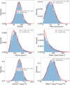 |
Fig. 17 Probability density functions of ruwe, UEVA, UEVA1/3, and PMa, PMa2 and PMa2/3 are modeled for a companion with mass 100 MJ and sma=1 au around a system similar to GJ 832 (i.e., an M-type star at parallax of 200 mas). Modeled data are shown in the blue histograms, and normal or χ2 laws are shown as red curves. The results of a Kolmogorov-Smirnov test statistics are shown in the legend. |
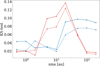 |
Fig. 18 Kolmogorov-Smirnov test statistics of the normal law with the distributions of UEVA and PMa (respectively red and blue solid lines) and UEVA1/3 and PMa2/3 (respectively red and blue dashed lines). |
7 The GaiaPMEX maps
7.1 Constraints from AEN, RUWE, and PMa on the mass and sma of a companion
We use the systems of GJ 832 and HD 114762 to illustrate the outcomes of the GaiaPMEX approach. Details on HD 114762 and GJ 832 are given respectively in Sects. 5.2 and 5.2.2 and their main parameters are summarized in Table B.1. Figs. 19 and 20 show the confidence regions, or maps, at confidence levels 68.3 (1−σ region), 95.4 (2−σ region), 99.73% (3−σ region), of the mass and sma of a candidate companion around GJ 832 and HD 114762 as calculated with GaiaPMEX, given either only ruwe or AEN – through calculating UEVA as explained in Sect. 5.1.1 – or only PMa, or combining the constraints from PMa and ruwe.
The maps give the possible sma and mass of a companion assuming it is responsible of the measured PMa, AEN or ruwe. The mass-sma degeneracy drawn by the confidence regions follows typical curves, essentially U-shaped for the PMa, and V-shaped for the AEN or the ruwe. They present mainly three features: a short-period (SP) branch, a long-period (LP) branch, and the near equal-mass binary solutions forming an horizontal branch around the mass of the primary (B-branch hereafter). The SP and LP semi-linear branches curve up into the B-branch because of the contribution of the secondary in the position of the photocenter. The GaiaPMEX combination of the constraints from PMa and ruwe, as shown on the green map in Figs. 19 and 20, combines the shape of the PMa and ruwe maps. Most importantly it lifts up a fraction of the degeneracy, leaving confidence regions of smaller extent.
In the case of GJ 832, as shown in Fig. 19, the αUEVA (AEN) maps form a confidence region at 2−σ leading to a mass >0.1 MJ with 95.4% confidence and a mass upper-limits at any sma <10 au. However, the ruwe is only leading to the 2−σ upper-limit on mass at any sma. This is explained by the difference in the significance of the αUEVA from either ruwe (1.7−σ) or AEN (2.5−σ). The PMa maps lead to a well-defined 3−σ confidence region with mass >0.5 MJ at 99.7% confidence and an upper-limit on mass within 1−40 au. Both 1−σ confidence regions of the αUEVA and PMa maps encircles the minimum mass 0.74 ± 0.06 MJ at sma=3.6 ± 0.4 au for GJ 832 b (Gorrini et al. 2022), as well as the mass of  MJ found by combining the RV and the Hipparcos-Gaia proper motions of GJ 832 in Philipot et al. (2023a). Nonetheless, the confidence regions still leave a lot of degeneracy in the sma and mass solutions. Combining the constraints from PMa and ruwe leads to reject most of the SP-branch. The remaining LP-branch spans ∼ 2−500 au with mass as low as 0.5 MJ. The 1−σ, or 68%, confidence region is restricted to within the LP-branch with sma=2-8 au and true mass within 0.5−2 MJ. Again, the 1−σ confidence region encircles the known possible mass and sma of GJ 832 b.
In the case of HD 114762, as shown in Fig. 20, the confidence regions drawn from AEN, ruwe and PMa agreed well on a companion mass >20 MJ for sma within 0.1−100 au. The ruwe and AEN even constrained sma to be lower than 20 au. Combining PMa and ruwe together led to still largely degenerated 2 and 3−σ confidence regions. The 1−σ region is now centered about 3 au and mass=50 MJ, and the 2−σ regions spans the stellar domain, embedding the known mass=225 ± 14 MJ at 0.38 au of HD 114762 b (Winn 2022). The wide-orbit companion at 130 au HD 114762 B cannot be compatible with neither Gaia nor Gaia-Hipparcos astrometry and thus did not contribute significantly to the photocenter’s motion as captured by Gaia.
The broken linear relationships drawn upon the U and V-shaped confidence regions in the PMa, AEN and ruwe maps are related to their physical interpretation. The semi-empirical laws behind those curves draw approximate constraints on the mass and sma for any system. We further elaborated on these insights in Sects. 7.2 and 7.3.
 |
Fig. 19 GaiaPMEX constraints on mass and sma of a candidate companion around GJ 832. Top-left: Using PMa. Top-right: using αUEVA from AEN. Bottom-left: using αUEVA from ruwe. Bottom-right: combining PMa and αUEVA. The colored regions inside the contours show the 68.3%, 95.4%, and 99.73% confidence intervals. The thick dark lines show the model relationships developed in Sects. 7.2 and 7.3. The yellow dot shows the properties of the known exoplanet companion in this system derived from RV, smab=3.6 au and Mb=0.99 MJ (Philipot et al. 2023a). |
7.2 The mass-sma relationship constrained by the αPMa
The typical broken U-shape of the mass-sma relationships that we found in the PMa map is shown in Fig. 19. It can be divided into four sections.
First, if P≫24.5 yr, then the HG baseline covers a part of the orbit. The contribution of the orbital motion in the HG PM vector and in the GDR3 PM vector are the mean orbital speed during respectively 24.5 and 3 yr. In this regime, the PMa is indeed an approximation of the orbital acceleration fixed by the relative sma of the companion, with PMa ∝ 1/sma2. This approximation is increasingly accurate with increasing orbital period, as the orbital motion becomes more linear within 24.5 yr. If P<24.5 yr, for an orbital period sufficiently small, the contribution of the orbital motion in the 24.5-yr averaged PM becomes negligible.
In fact, the central point between those two main regimes is close to a period of 49 yr, that is, about P/2=24.5 yr. Indeed, for a star on a pole-on circular orbit with P/2=24.5 yr, the orbital contribution to the HG PM (PMHG, orbit hereafter) that is, the average orbital speed along half the period, is ∼4 a*/P; the orbital contribution to the GDR3 PM (PMGDR3, orbit hereafter) is the instantaneous speed ∼ 2 π a*/P; and they lead to a ratio PMHG, orbit/PMGDR3, orbit ∼0.6. For P/2<24.5 yr, the orbital motion contribution to the PMHG, orbit becomes even smaller than half the orbital motion contribution to PMGDR3, orbit. Conversely, for P/2>24.5 yr, the PMHG, orbit and PMGDR3, orbit strengths gradually reach equality with increasing P.
Below 49 yr, assuming that PMHG, orbit becomes rapidly negligible, we find three different regimes that depend on GDR3 sampling and baselines at P<1 yr, 1<P<6 yr and 6<P<49 yr:
P<1 yr: The Gaia data undersample the orbits, leading to strong aliasing of the orbital signal. The fit proper motion varies a lot from one value of sma to another, and almost nulling at resonances between the main sampling frequency and the orbital frequency (see also Kervella et al. 2019). There is nonetheless an average trend of the αPMa that is linearly increasing with sma, and thus αPMa ∝ sma;
1<P<6 yr: Single orbits are better phase-covered, and there is more than half an orbit cycle monitored during the 3 yr of the GDR3. In this regime, the smaller the period, the more cycles are monitored and the less sensitive the αPMa is to the amplitude of the motion. Thus, αPMa ∝ sma P ∝ sma5/2;
6<P<49 yr: Less than half a phase of the orbital motion is covered by the Gaia observations and the fit proper motion is oriented along, and in intensity proportional to, the average orbital velocity of the star along this orbit segment. Thus, the αPMa is approximately proportional to the instantaneous orbital speed,
 .
.
 (31)
(31)
Those four regimes are all linear in log-log space but with different slopes. We note that the constraints stop following these linear models as the luminosity of the companion becomes comparable with the luminosity of the primary. When this occurs, as the luminosity of the companion increases, the photocenter semi-major axis shrinks more and more until reaching almost zero at a mass ratio15 q ∼ 1.
 |
Fig. 20 Same as Fig. 19 for HD 114762. The yellow dot shows the properties of the known massive companion HD 114762 Ab in this system, with smab=0.35 au and Mb=0.2 M⊙. The pink dot shows the wide binary companion HD 114762 B with smaB=130 au and MB=0.088 M⊙. |
7.3 The mass-sma relationship constrained by the αUEVA
We now explain the typical V-shape of the mass-sma relationship that we observed in the UEVA maps, that is, those of AEN and ruwe, shown in Fig. 19. Two regimes need to be distinguished. The regimes with P either shorter than 3 yr, when more than one orbital cycle is monitored, or longer than 3 yr, when only a part of a single orbit is covered by Gaia.
If P<3 yr, several orbital cycles happen during the GDR3 observation campaign. The residuals amplitude, and thus αUEVA, varies in proportion to the extent of the motion. The star’s semi-major axis a* itself is proportional to sma, αUEVA ∝ sma.
If P>3 yr, only a part of a single orbit is covered by GDR3’s observations and is locally fit by a linear motion. The αUEVA measures the non-linearity of the motion, that is, the acceleration. Therefore, in this regime, αUEVA ∝ 1/sma2.
 (32)
(32)
The log(mass) decreases linearly with the log(sma) down to about P=3 yr that corresponds to a range of sma within 1–3 au depending on the stellar mass. Then the log(mass) increases linearly with the log(sma) up to very long period, until it reaches stellar masses. We note that, as for the PMa, the constraints stop following these linear models as the luminosity of the companion becomes comparable with the luminosity of the primary, that is, beyond Mc∼0.5 M*.
7.4 The mass-sma relationships and the minimum mass of companion
The relations expressed above between Mc and sma, at given ϖ and M*, can be summarized as
 (33)
(33)
with ℓ a number indexing the considered period regime, Cℓ a multiplicative constant, and nℓ an exponent. To determine the Cℓ’s, we considered an arbitrary source and modeled by simulation 1000 values of αUEVA and αPMa at a P of the corresponding regime – either 0.1, 2, 30 or 100 yr – and at fixed Mc=10 MJ, M*=1 M⊙ and ϖ=1000 mas. The inclination, eccentricity and ω were set randomly following the distributions of Table 2. This led, for given sma=P2/3  , Mc, M* and ϖ, to distributions of αUEVA and αPMa, and thus, inverting Eq. (33), to measurements of the constants, Cℓ,simu ± σC,ℓ. Because this might lead to disconnected line segments at the transition between regimes, that is, at P=1, 3, 6, or 49 yr, we also imposed a continuity condition by noticing that from one regime ℓ to another contiguous ℓ + 1, there is a simple condition to fulfill:
 (34)
(34)
To do so, we minimized a least-squares problem by varying for either the case of αPMa or αUEVA only C1 and minimizing the following objective function f:
 (35)
(35)
where any Cℓ≠1 is determined by using Eq. (34) and, for example, log C3−log C1=(log C3−log C2) + (log C2−log C1). We expected that the Cℓ determined by this method would depend on the source considered due to the source-dependent noise levels, the shape of the unit parallax ellipse, and the Gaia and Hipparcos scan law. We thus used 20 arbitrary sources with diverse magnitudes, colors, and RA-DEC and determined their global average Cℓ rounded at the significant digit, given standard deviations of about 10−20%:
 (36)
(36)
 (37)
(37)
Reporting these numbers in Eq. (33), the curve segments in these different regimes are added to the GaiaPMEX maps in Figs. 19 and 20. Given the actual mass uncertainty associated with the maps at any sma, the Cℓ given here should only be considered as indicative, which is why we did not quote their uncertainties. These curves give an immediate approximate idea of what GaiaPMEX maps should look like without doing the full computation. They are not intended as a substitute for GaiaPMEX calculations. They do not produce, conversely to GaiaPMEX, exact constraints on the sma and mass of the companion given the observed AEN, ruwe and PMa. Nevertheless, these curves can allow for rapid estimation of the mass of the companion as a function of its possible sma given either AEN, ruwe, or PMa.
If the αUEVA or the αPMa are sufficiently significant, typically more than 2−σ, these relationships enable measuring of the minimum mass of the companion, located at the minimum of all curves. This is reached at an sma∼2–3 au:
 (38)
(38)
 (39)
(39)
These values can be used to identify planet candidates among catalogs of targets observed with Gaia.
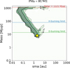 |
Fig. 21 Same as Fig. 19 but only showing the combined PMa+ruwe map for HD 81040. The known exoplanet companion is indicated as a yellow circle (see text). Individual maps from ruwe, AEN, and PMa constraints are shown in Appendix F, Fig. F.1. |
8 Illustrative cases of GaiaPMEX results
8.1 HD 81040: Evidence for a short-period companion
HD 81040 is well-known as being the system of the first discovery from GDR3 data of an exoplanet companion using only an orbital fit of the astrometric data (Gaia Collaboration 2023a)16. HD 81040 is a solar-type G2/3V star of magnitudes V=7.72 and G=7.57, at a distance of 32.56 ± 1.31 pc from Earth. The planetary candidate HD 81040 b was first discovered by Sozzetti et al. (2006) with an orbital period of 1001 days, eccentricity of 0.53 and an msin i of 6.86 MJ. Using the PMa calculated from the Gaia EDR3 and Hipparcos data, there was further indications that this companion was indeed planetary with a mass of  MJ (Li et al. 2021; Winn 2022). Ultimately, a joint fit of the astrometric GDR3 data and the RV data for this star fully confirmed a mass of
  MJ. At the orbital period, best constrained with RV, of 1001 days, the planet is predicted to have an sma=1.94±0.02 au (ref. Gaia ESA webpage).
Figure 21 shows the map constraining the mass and sma of a candidate companions around HD 81040 calculated with GaiaPMEX from combining ruwe and PMa constraints. Other individual maps using only AEN, ruwe and PMa are shown in the Appendix F, Fig. F.1. The parameters and results found for HD 81040 are summarized in Table B.1. The astrometric signatures of AEN and ruwe are both significant at >6.7−σ, with p-value∼0.00, while the αPMa cannot reject the single star hypothesis at a 1.5−σ significance and a p-value of 0.13. Nevertheless, the constraints on mass-sma calculated by GaiaPMEX from the PMa stay compatible with the known planet in this system, but do not strongly reject an edge-on inclination.
Most interestingly, when combining the constraints from the ruwe and the PMa, the LP-branch disappeared from the GaiaPMEX map, only leaving an SP-branch. The case of HD 81040 is thus illustrative of the identification by GaiaPMEX of a short-period companion, typically detectable using RV. Conversely, in such a case, it may allow for putting constraints on the mass of a known RV companion, as done with GASTON in Kiefer et al. (2019); Kiefer (2019); Kiefer et al. (2021). Here, the GaiaPMEX maps agree well with the mass and sma of HD 81040 b found by fitting the astrometric time series and the RV.
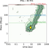 |
Fig. 22 Same as Fig. 21 but for AF Lep. There are supplementary figures in Appendix F, Fig. F.2. The known exoplanet companion is indicated as a yellow circle (Mesa et al. 2023). |
8.2 AF Lep: Evidence for a long-period companion
AF Lep is an F8V star, initially characterized as an RS CVn. It has been shown that its variability is actually due to the presence of a companion, a super-Jupiter with mass ∼3 MJ at 8 au, detected through the combination of astrometric acceleration and direct imaging (Franson et al. 2023; De Rosa et al. 2023; Mesa et al. 2023). The main parameters of AF Lep are summarized in Table B.1. This system was selected for follow-up with direct imaging because it shows a significant astrometric acceleration, or PMa, compatible with a planet mass. This was a long-shot, because using PMa only, one cannot reject that this system is actually a short period binary that would remain unresolved by direct imaging, while lower mass or lower sma could remain plausible, also leading to a non-detection with direct imaging.
The GaiaPMEX maps obtained for AFLep are shown in Figs. 22 and F.2. In agreement with previous work on this source, the astrometric signature of the PMa is significant at 4−σ, that is, compatible with the single star hypothesis with a p-value of 6.334 × 10⁻⁵. Both astrometric signatures found for AEN and ruwe cannot reject the single star hypothesis for AFLep with a p-value of 0.96 and a significance <0.1−σ. It leads to strict upper-bounds on the companion mass at any sma, since otherwise the AEN and ruwe would have been more significant.
Interestingly, the mass-sma constraints from PMa are largely degenerate, but combining them with those from ruwe leads to rejection of most low-sma solutions, that is, the SP-branch.
This shows that combining the PMa and the ruwe would have led to much tighter constraints on the possible mass and sma of a companion around AFLep. The detected companion with  MJ at sma=7.99+0.85 au using direct imaging (Mesa et al. 2023; Franson et al. 2023) falls indeed within the 1−σ bounds of the LP-branch.
8.3 HD 23596: An almost detection with astrometry
HD 23596 is a V=7.2-mag F8 star at 52 pc from the Sun that is known to host a companion planet. It was first discovered as an 8.2−MJ super-Jupiter with the ELODIE spectrograph (Perrier et al. 2003) and further characterized with a similar msini by Wittenmyer et al. (2009) (7.71±0.39 Mj) and Stassun et al. (2017) (9.03±0.74 MJ) using supplementary High Resolution Spectrograph (HRS) data and new M* estimations. It was then re-established as a 14−MJ low-mass brown dwarf combining RVs and Hipparcos-Gaia PMa (Feng et al. 2022; Xiao et al. 2023). The orbital period of this companion is  years, with an sma of 2.90 ± 0.08 au, a mass of
  MJ and an inclination being of either
  (prograde) or
  (retrograde) (Xiao et al. 2023). The inclination significantly non edge-on explains the lower 8.2-MJ m sin (i) initially found for this companion.
The GaiaPMEX analysis combining the constraints from both ruwe and PMa of HD 23596 led to the confidence regions on companion mass and sma shown in Fig. 23. The individual maps from either ruwe, AEN or PMa contraints are shown in the Appendix in Fig. F.3. The combination of PMa and ruwe leads to infer a companion in the brown dwarf domain, with a narrow constraint on mass within 10−30 MJ as well as on sma within 2–5 au at 68.3% confidence. This is in perfect agreement with the known companion of HD 23596. Surprisingly, this source was not identified as a non-single star and does not appear in the non-single star catalog (Gaia Collaboration 2022)17. This shows that Gaia in combination with Hipparcos, with the help of the GaiaPMEX tool, can detect and characterise a companion even without including RVs. More such planet candidates with strong constraints on the mass and the sma from only Gaia + Hipparcos astrometry will be presented in other forthcoming papers (paper II, Kiefer et al. 2025; paper III, Lagrange et al. 2024).
8.4 α CMa B: The effect of considering a dark companion
The case of α CMaB is an instructive opportunity to show the effect of considering either a dark or a non-dark companion in the GaiaPMEX analysis. Indeed, α CMa B is nothing else than Sirius B, the white dwarf companion of the massive 240 Myr old Sirius. It was first hypothesized by Bessel (1844), then officially discovered by A. G. Clark in 1862, and further characterized by Flammarion (1877). Even though its average separation with Sirius A is only 19.6 au, the close distance to the Sun of this system lead to an angular separation of 7.6′′ (van den Bos 1960), and thus Sirius B was resolved in the GDR3. The respective mass of Sirius A & B are 2.14 M⊙ and 1.05 M⊙ (Gatewood & Gatewood 1978). Based on the orbital analysis of the Sirius AB system using astrometry, an additional companion Sirius C around either A or B was suspected to exist in this system, with a putative orbital period of 6 years (Volet 1932; Benest & Duvent 1995). Around Sirius B’s, this companion may have a mass <20 MJ and an orbit sma of 1–2.5 au (Bonnet-Bidaud & Pantin 2008). Using Keck/NIRC2 observations, Lucas et al. (2022) further excluded any companion of mass >10 MJ down to 0.2 au, >2.4 MJ down to 0.5 au and >0.7−1.2 MJ beyond 1 au around Sirius B.
In GDR3, as summarized in Table B.1, the αUEVA, from both AEN and ruwe, of Sirius B is significant, >9−σ. Sirius B was not observed with Hipparcos, implying no PMa for this star. The map derived from ruwe is shown in Fig. 24. We considered, by default in the top figure, a luminous companion. Within Lucas et al. (2022) constraints, the ruwe allows at 2−σ for a companion with a mass as high as 10 MJ at less than 0.5 au. However, with a mass ∼2.1 M⊙, the known companion of Sirius B, that is, Sirius A, at an average sma∼20 au, seems to explain the observed ruwe without the need to invoke a supplementary companion.
Nonetheless, for Sirius A, this approach is problematic for two reasons. First, the age of the system is overestimated since in the current version of GaiaPMEX, the mass-luminosity relation is determined only for an age of 5 Gyr. Second, and most importantly, even though it is much more luminous than B, Sirius A is well resolved by Gaia and cannot act in the position of the photocenter of Sirius B. The main effect of considering dark or luminous companion is to change the shape of the confidence region at companion mass on the order of the magnitude of the mass of the source, here 1.05 M⊙. A luminous companion narrows down the photocenter’s orbit. For a given constant photocenter semi-major axis, at short periods it requires the companion’s sma to increase, while at long periods it requires the acceleration to increase and thus the sma to decrease. Considering instead a companion whose light does not contribute to the photocenter (dark or resolved), the confidence region rather more closely follows the curves derived in Sects. 7.3 and 7.2 that only describe the reflex astrometric motion of the main source under the gravitational pull of a companion.
The GaiaPMEX map derived from ruwe for Sirius B and considering a dark companion is shown in Fig. 24, bottom. We note that Sirius A is within the 3−σ region and upon the edge of the 2−σ region. Thus, we confirm that Sirius A may indeed explain the ruwe, although it would tend to generate, on average, a ruwe larger than the one published in the archives.
Finally, the GaiaPMEX maps of Sirius B cannot exclude any companion with a mass located below the confidence regions, since the perturbation from this other companion would be subdominant. It thus remains possible that another hidden companion exist around Sirius B. The IPD_frac_multi_peak and IPG_gof_harmonic_ampl of α CMaB are moderate, respectively 18% and 0.05, but according to our analysis performed in Appendix C, they imply that a source within 200–500 mas, that is, 0.5−1.3 au, with a flux ratio within 10−4−10−3 is acting on the shape of the PSF. Interestingly, the Lucas et al. (2022) analysis allows for a <1−2 MJ companion at 0.5−1.3 au below a limiting contrast of ∼10−3. This strongly suggest digging further within the 1-au surroundings of the white dwarf Sirius B in the quest of planets.
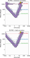 |
Fig. 24 Same as Fig. 19 for α CMa B but only showing the constraints from ruwe since it was never observed with Hipparcos. Top: considering a luminous companion with both components at age ∼5 Gyr. Bottom: considering a dark companion. |
8.5 β Pictoris: An issue with the RUWE
We focus here on the system of β Pictoris to bring forward again that the ruwe and AEN cannot be interpreted directly as binarity indicators, but only through determining the astrometric signature within residuals and its significance. The main parameters of β Pictoris are summarized in Table B.1. β Pictoris is a south-hemisphere 20-Myr old A5V star (Mamajek & Bell 2014) located at 19.6pc from the Sun with a G-mag of 3.82. It is known for being the most furbished planetary system, after the Solar system, in the wealth of body types that planet formation can produce. It hosts a widely extended dusty and gaseous debris disk, exocomets, asteroids, and giant exoplanets with masses of ∼8 and ∼10 MJ. It is a system of great importance and a focus of attention from the community for understanding the running processes during the first hundred Myr of the Solar system and of planetary systems in general. In the GDR3 database, β Pictoris is announced with a ruwe of 3.07 and an AEN of 1.39 mas. It looks therefore at first sight that significant deviation to the five-parameter model has been detected in this system, if we follow the guidelines that ruwe>1.4 indicates a non well-behaved or non-single system (as recommended in the DR3 documentation). However, here it is not the case.
At a  for 231 good AL measurements, the UWE for β Pic is 17.2 and seems anomalously large, apparently corroborating the large ruwe. Considering the level of noises for this bright blue source of the 6p-dataset that we found in Sect. 3, that are σcalib=1.548 mas, σAL=0.012 mas, and σAL=0.074 mas, the χ2 expected for a single source according to Eqs. D.8 and D.9 is 80 000±24 000. And it corresponds to UWE=18.8 ± 2.8, in good agreement with the value found above, indicating that 17.2 is, in fact, not an anomalously large UWE. It is therefore surprising that the ruwe of β Pic is 3 times larger than 1.0, while the ruwe was introduced as a renormalized version of the UWE to recenter this goodness-of-fit indicator around unity for well-behaved sources. The renormalizing factor u0 in Eq. (3) is thus ill-defined for sources in the 6p-dataset at the (G, Bp − Rp) corresponding to β Pic, that is, at G=3.82 and Bp − Rp=0.261. The AEN=1.39 mas is conversely well defined for β Pic. According to the relation of Eq. (7), the AEN implies
  . This is in good agreement with the value expected for a single star determined above. The astrometric signature derived from AEN and ruwe is undefined because their corresponding UEVA are smaller than the single star’s expected UEVAsingle in Eq. (27).
Figure 25 compares the UWE obtained for single stars from Eq. (D.8) to the u0 found in the GDR3 auxiliary data18 over the whole sources database with G<16. The ratio of both quantities is ruwesingle, that should ideally be equal to 1. The distribution of this ratio peaks indeed at 1, but in the 6p-dataset, there are strong tails on both sides toward lower and higher values. In the 5p-dataset, some ruwesingle deviate from 1, although much tightly than in the 6p-dataset. In the 5p dataset, 462 over 71 042 992 sources (6.510−4%) have a ruwe >1.4, while in the 6p dataset there are 14 890 over 2 203 807 sources (0.68%) with a ruwe >1.4. In conclusion, regardless of the dataset, it is safer to interpret the values of AEN and ruwe only through calculating the astrometric signature of the UEVA, as defined in Sect. 5.1.
The GaiaPMEX maps of β Pictoris are shown in Fig. 26. Consistently with the above analysis, the AEN and ruwe both lead to sma and mass of a hypothetical companion to β Pic compatible with a single star, that is, mass=0 MJ or sma=0 au. The two planets (b: 10−11 MJ at 9.8±0.4 au; c: 7.8±0.4 MJ at 2.7±0.02 au; Lagrange et al. 2020) are compatible with the AEN and ruwe, as well as the PMa. There are no evidence in the GDR3 for any other yet unknown companion around β Pictoris.
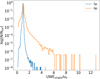 |
Fig. 25 Statistics of the ratio of the single star’s UWE over the u0 published for all sources with G<16. Sources are separated into 5p and 6p datasets. |
9 The current sensitivity of Gaia to the presence of companions
We determined the detection rates of exoplanets of different mass and sma that one can expect from using either PMa, UEVA (determined from AEN or ruwe), or PMa ∪ UEVA19. They strongly depend on the stellar mass M* and parallax ϖ. We call “detection” any value of αUEVA or αPMa more significant than 2−σ, that is, for which the UEVA1/3 or the PMa2/3 are above the 95.4th percentile of the respective single star’s distributions.
Considering pre-main to main-sequence (MS) stars, we explored a 2D-grid, with 30 bins per dimension uniformly spaced in log-scale, of M* from 0.08 to 2.5 M⊙ and ϖ from 1 to 1000 mas. At each bin with given (M* ± ΔM*, ϖ ± Δϖ), we modeled UEVA and PMa by simulation (see Sect. 4) of photocentric orbits as observed by Gaia and Hipparcos, due to companions with a mass Mc within bins delimited by 0.1, 0.2, 0.51, 2, 5, 10 and 20 MJ and with an sma within different orbital regimes: Mercury-Earth type (0.1−1 au), Earth–Mars type (1−3 au), Jupiter-Saturn type (3−10 au) and Uranus-Neptune type (10−30 au). The G-mag and the Bp − Rp color corresponding to a given M* and ϖ are calculated from Pecaut et al. (2012) and Pecaut & Mamajek (2013)’s spectral type to flux conversion tables for pre-MS to MS stars20. The absolute magnitude MG is converted to apparent magnitude G using the distance modulus calculated from the parallax. For simplicity, and to draw the general picture, we assumed zero extinction. The results are thus susceptible to be only informative, especially beyond 100 pc. We fixed the other properties (such as RA, Dec, parallax unit ellipse, Hipparcos IADs) and the GDR3 epochs sampling, to those of GJ 832. At each bin, the noises σcalib and σAL levels are fixed with respect to the median G and Bp − Rp. Since our initial sample covers 3 to 16 G-mags, our study of sensitivity in GDR3 is limited to this range.
For each bin, we simulated N=1000 orbits given the range of companion sma and Mc and host star’s M* and ϖ, randomizing other orbital parameters according to the distributions defined in Table 1. We counted the percentage r – or detection rate – of UEVA1/3 and PMa2/3 exceeding the 95.4th-percentile in their respective single stars’ distributions. We determined when r>20, 50, 90 and 99%. We were peculiarly interested in the possibility to detect a planet by considering PMa, UEVA or both, that is, PMa ⋃ UEVA. For single stars, the frequency of FP beyond the 2−σ threshold is 4.6%, when PMa or UEVA are considered separately, and 9.2%, when considering PMa ⋃ UEVA. This is the worst case scenario (largest FP frequency) in which noise rather than orbital motion causes a significance larger than 2−σ. In the general case, some true companion detections might be serendipitous, that is, due to noise rather than orbital motion, and it is not possible to determine exactly the fraction of FP in this case. At best, a percentage r>4.6% (respectively 9.2%) indicates an increased sensitivity of Gaia to the detection of companions in the given range of mass and sma. At worst, the fraction of FP is 4.6/r (respectively 9.2/r). In particular, if r is close to 4.6% (respectively 9.2%), then the fraction of FP is close to 100%.
A map of the detection rates – or equivalently, Gaia's sensitivity to companion detection – with respect to star mass and parallax from using PMa, αUEVA or both is shown in Fig. 27. Planets with mass <1 MJ around stars located farther than 100 pc (ϖ<10 mas) from the Sun lead to significant astrometric signal in less than 20% of the simulations. But Jupiter-mass planets (1−2 MJ) might be detected with a >20% chance around stars less massive than 1 M⊙ and up to 100 pc distance. Similarly, planets of mass <0.1 MJ around solar-like stars (0.5−2 MJ) have a less than 20% chance of detection with Gaia whatever their sma and whatever the distance to the Sun. But, if their host is an M-type star closer than 10 pc and if their sma is within 1−10 au, planets of any mass >0.1 MJ have a more than 20% chance of being detected at 2−σ. Moreover, within 1−10 au and if their host star is an M-type star closer than 5pc, Jupiter-mass planets (1−2 MJ) were detected in >99% of simulations, and Neptune/Saturn-mass planets (0.1−0.2 MJ) in >50% of the simulations. Finally, super-Jupiter and brown dwarfs are easily detected at a rate >99% up to large distance, even beyond 100 pc and around A-type stars with M*>2 M⊙.
Focusing now on close-by low mass stars, we invoked again GJ 832, a 5-pc distant M-dwarf, and derived the maps of Gaia's sensitivity to companion detection around this star. We modeled the UEVA and PMa on a grid of sma and Mc, the same that was used for the GaiaPMEX constraints maps, and determined the detection rates r, as done above. The map for detection with UEVA ⋃ PMa is shown in Fig. 28 and the individuals maps for detection with either UEVA or PMa are shown in Fig. G.3. Around such a star, super-Jupiter and brown dwarfs with mass >10 MJ and with an sma within 0.2–20 au are detected in >99% of the simulations. Lighter planetary companions whose mass is within 2−10 MJ may lead to a significant astrometric signal in >99% of the cases, provided their sma is contained within a narrower range of 1−10 au. At masses in the Saturn-to-Jupiter regime (0.2−1 MJ) planetary companions have a lower detection rate, with a >50% chance of being detected for an sma within 2−10 au. Planets of mass <0.2 MJ are much less frequently detected (<50%) whatever their sma. The detection rates obtained when considering only PMa or only UEVA (Fig. G.3) show that the PMa is more sensitive to planets orbiting in the 2−20 au range, while the UEVA tends to perform the most efficiently at shorter separations from 0.2 to 2 au.
In summary, GDR3 currently performs best at detecting sub-stellar companions that are more massive than Jupiter on Earth-to-Saturn orbits (1−10 au) around any star closer than 100 pc from the Sun.
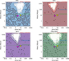 |
Fig. 26 GaiaPMEX constraints on mass and sma of a candidate companion around β Pictoris. Same caption as Fig. 19. The yellow and pink dots show the properties of the known exoplanet companions b & c in this system, with smab=9.8 ± 0.4 au and mb=10−11 MJ, and sma smac=2.7 ± 0.02 au and Mc=7.8 ± 0.4 MJ (Lagrange et al. 2020). |
10 Conclusion
We have introduced GaiaPMEX, a tool that allows for characterization of the possible mass and sma of companions to stars observed with Gaia. It uses the proper motion anomaly (PMa) and the excess of the five-parameter model residuals, the unbiased estimator of variance a posteriori (UEVA), indicated by the values of renormalized unit weight error (ruwe) or astrometric excess noise (AEN). GaiaPMEX determines their significance with respect to the null hypothesis of a single star by calculating an astrometric signature for each indicator, αPMa and αUEVA, and then models them by the star’s reflex motion due to a companion with ranges of possible mass and sma.
Being otherwise highly degenerate in mass and sma, by combining the use of AEN or ruwe and PMa, the space of solutions is significantly reduced. This has never been done before and is highly promising for characterizing systems also observed by other means (radial velocities mostly). When αUEVA or αPMa are significant, the posterior maps follow mass-sma relationships that are given in Eqs. (36) and (37) and that vary with orbital periods. Thereby, the PMa could only be considered as a proxy for orbital acceleration when the orbital period of the companion is longer than 49 yr, while the UEVA varies positively with the photocenter semi-major axis only when the orbital period of the companion is shorter than 3 yr.
We determined companion detection rates and Gaia's sensitivity to exoplanet detection by comparing modeled UEVA and PMa for companions with a hypothesized mass and sma to expectations for single stars. We show that in the exoplanet domain, the best detection rates are obtained for M-dwarf sources that are closest to the Sun (<10 pc) and for exoplanet’s sma within Earth-to-Saturn orbits, that is, 1−10 au with masses down to 0.1 MJ.
In the present article, we introduced in greater detail the GaiaPMEX tool and the needed estimation of calibration, attitude and measurement noise levels. We plan on extensively exploiting GaiaPMEX for the search and characterization of exoplanets in further studies.
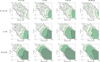 |
Fig. 27 Theoretical detection rates with respect to M* and the parallax. We varied the mass and the sma of the companion according to the column and row labels. White regions show the M* and the parallax for which the probability of companion detection is less than 10%; darker green regions show a probability of detection of >20%,>50% and >99%. The dashed lines show the M*-parallax relations at the limiting magnitudes of G=3 and G=16 derived from Pecaut & Mamajek (2013) tables. Similar figures are obtained considering only ruwe or PMa in Appendix G, in respectively Fig. G.1 and G.2. |
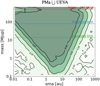 |
Fig. 28 Theoretical Gaia detection rates of companions with a given mass and sma around GJ 832 as permitted by allowing a detection with PMa ∪ UEVA. White regions show the mass and sma for which the probability of detection of the companion is less than 10%; dark green regions show a probability of detection >99%; light green regions have intermediate probabilities. Individual maps for UEVA and PMa are shown in Fig. G.3. |
Data availability
Appendix E–H are available at the following url at https://zenodo.org/records/17192804?token=eyJhbGciOiJIUzUxMiJ9.eyJpZCI6ImFkYWV1NDg1LTQzMmQtNDczZC1hNzk3LWYzYzUwNmYxZjE1MSIsImRhdGEiOnt9LCJyYW5kb20iOiIyNjRlN2QyYjczOWRhODVlMjc1NmU1NjlhNjQ2MmFlMyJ9.n8FLZELuZ80ifu1hqDkJ6svxBxeBxmsDauL3LmlGmDVv50Jk3FxKYF4KuYMO_2ExMNdHpB4LkSpvN_urjrCLuw
Acknowledgements
We are very thankful to the anonymous referee for her/his thorough and courageous reading that led to significant improvements of this article. This work has made use of data from the European Space Agency (ESA) mission Gaia (https://www.cosmos.esa.int/gaia), processed by the Gaia Data processing and analysis consortium (DPAC, https://www.cosmos.esa.int/web/gaia/dpac/consortium). Funding for the DPAC has been provided by national institutions, in particular the institutions participating in the Gaia Multilateral Agreement. This work was granted access to the HPC resources of MesoPSL financed by the Region Ile de France and the project EquipMeso (reference ANR-10-EQPX-29-01) of the programme Investissements d’Avenir supervised by the Agence Nationale pour la Recherche. This project has received funding from the European Research Council (ERC) under the European Union’s Horizon 2020 research and innovation programme (COBREX; grant agreement no. 885593). F.K. acknowledges funding from the initiative de recherches interdisciplinaires et stratégiques (IRIS) of Université PSL “Origines et Conditions d’Apparition de la Vie (OCAV)”, as well as from the Action Pluriannuelle Incitative Exoplanètes from the Observatoire de Paris – Université PSL. F.K. also acknowledges funding from the American University of Paris.
Appendix A Table of acronyms used in the text with their definitions and page references
| Notation | Description | Page List |
|---|---|---|
| 5p | five parameters | 4, 6, 7, 10, 11, 22, 29, 30 |
| 6p | six parameters | 4, 6, 7, 10, 11, 22 |
| AC | across scan | 2, 7 |
| AEN | astrometric excess noise | 1–4, 6, 9–14, 16–22, 25 |
| AL | along scan | 2–4, 6–10, 22, 29, 30 |
| BD | brown dwarf | 1 |
| CU8 | Coordination unit 8 | 13 |
| DEC | declination | 2–5, 8–11, 23 |
| DOF | degree of freedom | 2, 15 |
| DPAC | Data processing and analysis consortium | 25 |
| DR | data release | 1, 2, 6 |
| FLAME | final luminosity age and mass estimate | 13 |
| FP | false-positives | 12, 23, 24 |
| FoV | field of view | 6–11, 30 |
| GASTON | Gaia astrometric noise simulation to derive orbital inclination | 6, 20 |
| GDR3 | third Gaia data release | 1–13, 15–19, 21–24, 28–30 |
| GOST | Gaia observation forecast tool | 7, 8 |
| GaiaPMEX | Gaia DR3 proper motion anomaly and astrometric noise excess | 1–3, 14–17, 19–25 |
| HG | HIPPARCOS–Gaia | 3, 8, 9, 12, 14–17 |
| IADs | intermediate astrometric data | 8 |
| ICRS | International celestial reference system | 3,4 |
| IPD | Image parameter determination | 29 |
| LR | likelihood ratio | 15 |
| LSF | line spread function | 29 |
| MAD | median absolute deviation | 6 |
| MCMC | Markov-chains Monte-Carlo | 13 |
| MS | main-sequence | 22, 23 |
| PA | position angle | 3,7,8 |
| probability density function | 14 | |
| PMa | proper motion anomaly | 1–3, 6, 8, 9, 11–25 |
| PSF | point spread function | 4, 22, 29 |
| RA | right ascension | 2–5, 81, 23 |
| RMS | root mean square | 29 |
| RSE | regression standard error | 9, 10, 29 |
| RSS | residuals sum of square | 2 |
| ruwe | renormalized unit weight error | 1–3, 6, 9–14, 16–22, 24, 25, 29 |
| RV | radial velocity | 1, 16, 17, 19, 20 |
| S/N | signal-to-noise ratio | 13 |
| sma | semi-major axis | 1–3, 6, 12–25 |
| UEVA | unbiased estimator of variance a posteriori | 9–19, 21–25, 29 |
| UWE | unit weight error | 6, 22 |
| WC | window class | 4 |
| WFS | wavefront sensor | 7, 8 |
Appendix B Additional table
Parameters for the illustrative cases discussed in this paper.
Appendix C The Gaia point and line spread function variations
The Image parameter determination (IPD) of Gaia makes a fit by a single point spread function (PSF; line spread function or LSF, if G>13) of the flux distribution within some defined window around any source transiting the detector. When polluting light is present and not masked out, it periodically affects the location of the measured photocenter compared to the theoretical photocenter at the light-barycenter of the main targeted source. The presence of unresolved sources (background or wide-orbit companions) nearby may thus cause undesirable variable shifts of the photocenter of the main source. The amplitude of the shifts is correlated with the angle between the AL scan direction (with position angle ψ) and the lines joining the polluting sources and the main source (with position angle θ).
The IPD_frac_multi_peak indicator published in the GDR3 archive gives the information on the fraction of exposures for which multiple modes have been detected. The window is then recalculated by masking out the parts containing the identified peaks (Holl et al. 2023). In theory, since some peaks may not be detected and masked out at all epochs, this can be a source of supplementary spurious variations in the 5p-fit residuals. These spurious variations are partly removed by the Gaia's reduction software. It fits a sinusoidal function of the angle of the AL scan direction ψ (a.k.a subpixel phase; Lindegren et al. 2021) to the astrometric time series of the targeted source (c + a sin ψ + b cos ψ; Eq. 9 in Lindegren et al. 2021). The shift function is not a perfect sinusoid due to the non-axisymetric shape of the PSF on the detector (Holl et al. 2023). Thus, a residual AL angle Δ η remains that may vary through time and mimick the signature of true orbital astrometric motion. The IPD produced another important indicator of PSF distortion, the IPD_gof_harmonic_amplitude. It measures the amplitude of the sinusoidal variation of the goodness-of-fit  of the PSF (LSF) fit. Fabricius et al. (2021) showed that sources with a ruwe indicative of possible binarity, and IPD_frac_multi_peak>2 or the IPD_gof_harmonic_amplitude>0.1, must be considered as resolved doubles.
We modeled the observation by Gaia, through time, of two Gaussian PSF of a wide-orbit binary, that is, with virtually no orbital motion during Gaia's 3-yr monitoring. We assumed separations ranging from 0 to 1000 mas and flux ratio of 0.001−1. An example is shown in Fig. C.1. We fixed the CCD noise to 1% of the flux, corresponding to AL measurement uncertainty of ∼0.03 mas. We arbitrarily fixed the flux at the tip of the PSF of the main source to 1. We fit the double star PSF by a single 2D-Gaussian varying only the scale and the centroid locus. A fit result is also shown in red in Fig. C.1. We obtained series of GOF and photocenter AL angle that we fit by a sinusoidal function following the AL scan rotation law, leading to GOF variation amplitude and residual Δ η beyond the five-parameter model. Figure C.2 shows the root mean square (RMS) of Δ η with respect to separation and flux ratio, as well as some isocontours of IPD_frac_multi_peak (at 2 and 98%) and IPD_gof_harmonic_amplitude (at 0.1 and 1%).
We found that significant residuals are associated with IPD_frac_multi_peak being different than 0 or 100% or with IPD_gof_harmonic_amplitude being larger than 0.1, while, insignificant variations on the order of the AL measurement uncertainty were mostly found when IPD_frac_multi_peak is close to 0 or 100% and IPD_gof_harmonic_amplitude<0.1. This agrees well with Fabricius et al. (2021) conclusions, but shows also that for fully resolved binary the IPD PSF fit remains unperturbed. As long as IPD_gof_harmonic_amplitude<0.1 and IPD_frac_multi_peak < 2 or >98%, the astrometric signature αUEVA is only lightly affected by the binary astrometric bias and correctly measures supplementary astrometric motion. However, for the sources that do not comply to these conditions, the interpretation of αUEVA, as indicative of orbital motion of the photocenter, is hazardous.
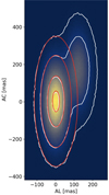 |
Fig. C.1 Simulation of the IPD fit of a 2D Gaussian PSF on a wideorbit binary with separation of ∼200 mas and a flux ratio of 0.42. |
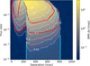 |
Fig. C.2 Photocenter centroid variations RSE with respect to binary separation and flux ratio delineated with white contours. The red contours delineate the GOF amplitude (at levels 0.1 and 1) and the cyan contours delineate the 2 and 98% levels of the IPD_frac_multi_peak. The white hatched region shows, as discussed in the text, where the RMS of the Δη residuals could be larger than 0.1 mas, while outside this region it is always <0.1 mas. |
Appendix D Detailed calculation of the approximate probability density function followed by 
We show here that for a single star, the  that can be found in the GDR3 archive does not actually follow a χ2 distribution with N−5 degree of freedom. Instead we show that it more accurately follows a linear combination of normal distributions. The
  is expressed with respect to the residuals of the five-parameter astrometric fit:
 (D.1)
(D.1)
where as assumed in the rest of this paper, the formal error σℓ ≡ σf is approximately constant throughout all data points. The formal error is the quadratic sum  (Lindegren et al. 2012) with σatt the attitude excess noise (see Appendix 3.2) and σAL the along-scan measurement error (see Appendix 3.3). The formal error is explicitly calculated for each GDR3 source in Appendix 3.1. One residual Rℓ is the sum of two contributions ri and
  , with ri that varies randomly from one FoV transit (i) to another with normal distribution
  (0, σcalib), and
  that varies for a given FoV transit (i) from one AL measurement (j) to another with normal distribution
  . It follows that
 (D.2)
(D.2)
We recall that NFoV is the number of FoV transits on the detector, and NAL is the average number of AL angle measurements per transit, that is, NAL=int(N/NFoV), given N is the astrometric_n_good_obs_AL. And thus  is the combination of three terms:
 (D.3)
(D.3)
with
 (D.4)
(D.4)
 (D.5)
(D.5)
 (D.6)
(D.6)
The last term Z is obtained as the sum of the product of two normally distributed variables:
 (D.7)
(D.7)
The standard deviation of the product of two normally distributed variables centered on zero is the product of their standard deviation, and the standard deviation of the sum of normally distributed variables is the root sum square of their standard deviation. This leads us to the formula of Z expressed in Eq. D.6, given moreover that the total number of astrometric points is N ≈ NAL NFoV. The two first terms X and Y dominate the spread, thus  should mainly be distributed according to a skewed χ2 law. Thus,
  follows a quasi-normal distribution
  (μ, σ) with
![Mathematical equation: $\mu = \frac{N_{{AL}}}{\sigma^{2}_{\rm{att}}+\sigma_{\rm{AL}}^2}\,\left[(N_{\text{FoV}}-5) \, \sigma_{\rm{calib}}^2 + N_{\text{FoV}}\,\sigma^{2}_{\rm{AL}}\right]$](/articles/aa/full_html/2025/10/aa49335-24/aa49335-24-eq114.png) (D.8)
(D.8)
![Mathematical equation: $\begin{align} \sigma^2=& \frac{2 N_{{AL}}}{\left(\sigma^{2}_{\rm{att}}+\sigma_{\rm{AL}}^2\right)^2}\,\Bigg[ N_{{AL}} \left(N_{\text{FoV}}-5\right)\,\sigma_{\rm{calib}}^4 \\ & \qquad\qquad\qquad + N_{\text{FoV}}\,\sigma^4_{\rm{AL}}\\ & \qquad\qquad\qquad + 2\,N_{\text{FoV}} \,\sigma_{\rm{AL}}^2\,\sigma_{\rm{calib}}^2\Bigg].\end{align}$](/articles/aa/full_html/2025/10/aa49335-24/aa49335-24-eq115.png) (D.9)
(D.9)
We compared the simple χ2 distribution with N − 5 degrees of freedom and this non-trivial normal model to the distribution of 10,000  values modeled for a single source from the 5p dataset in Fig. D.1. Models are obtained by simulation, as explained in Sect. 4 by generating noisy astrometric measurements of GJ 832 by Gaia, assuming zero orbital motion, and fitting-out a five-parameter model, leading to residuals Rℓ and a χ2 as defined in Eq. D.1. We indeed found that the non-trivial normal distribution is a more accurate model of the true probability law that is followed by
  , than a naïve χ2-law.
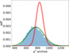 |
Fig. D.1 Distribution of |

References
- Babusiaux, C., Fabricius, C., Khanna, S., et al. 2023, A&A, 674, A32 [NASA ADS] [CrossRef] [EDP Sciences] [Google Scholar]
- Bailey, J., Butler, R. P., Tinney, C. G., et al. 2009, ApJ, 690, 743 [Google Scholar]
- Benest, D., & Duvent, J. L. 1995, A&A, 299, 621 [NASA ADS] [Google Scholar]
- Bessel, F. W. 1844, MNRAS, 6, 136 [Google Scholar]
- Bonnet-Bidaud, J. M., & Pantin, E. 2008, A&A, 489, 651 [EDP Sciences] [Google Scholar]
- Brandt, T. D. 2021, ApJS, 254, 42 [NASA ADS] [CrossRef] [Google Scholar]
- Brandt, T. D., Dupuy, T. J., & Bowler, B. P. 2019, AJ, 158, 140 [Google Scholar]
- Calabretta, M. R., & Greisen, E. W. 2002, A&A, 395, 1077 [NASA ADS] [CrossRef] [EDP Sciences] [Google Scholar]
- Canal, L. 2005, Computat. Statist. Data Anal., 48, 803 [Google Scholar]
- Cochran, W. D., Hatzes, A. P., & Hancock, T. J. 1991, ApJ, 380, L35 [NASA ADS] [CrossRef] [Google Scholar]
- Dalal, S., Kiefer, F., Hébrard, G., et al. 2021, A&A, 651, A11 [NASA ADS] [CrossRef] [EDP Sciences] [Google Scholar]
- De Rosa, R. J., Nielsen, E. L., Wahhaj, Z., et al. 2023, A&A, 672, A94 [NASA ADS] [CrossRef] [EDP Sciences] [Google Scholar]
- Fabricius, C., Luri, X., Arenou, F., et al. 2021, A&A, 649, A5 [NASA ADS] [CrossRef] [EDP Sciences] [Google Scholar]
- Feng, F., Butler, R. P., Jones, H. R. A., et al. 2021, MNRAS, 507, 2856 [NASA ADS] [CrossRef] [Google Scholar]
- Feng, F., Butler, R. P., Vogt, S. S., et al. 2022, ApJS, 262, 21 [NASA ADS] [CrossRef] [Google Scholar]
- Flammarion, C. 1877, Astron. Reg., 15, 186 [Google Scholar]
- Franson, K., Bowler, B. P., Zhou, Y., et al. 2023, ApJ, 950, L19 [NASA ADS] [CrossRef] [Google Scholar]
- Gaia Collaboration (Prusti, T., et al.) 2016, A&A, 595, A1 [NASA ADS] [CrossRef] [EDP Sciences] [Google Scholar]
- Gaia Collaboration (Brown, A. G. A., et al.) 2021, A&A, 649, A1 [NASA ADS] [CrossRef] [EDP Sciences] [Google Scholar]
- Gaia Collaboration 2022, Gaia DR3 Part 3. Non-single stars [Google Scholar]
- Gaia Collaboration (Arenou, F., et al.) 2023a, A&A, 674, A34 [CrossRef] [EDP Sciences] [Google Scholar]
- Gaia Collaboration (Creevey, O. L., et al.) 2023b, A&A, 674, A39 [CrossRef] [EDP Sciences] [Google Scholar]
- Gatewood, G. D., & Gatewood, C. V. 1978, ApJ, 225, 191 [Google Scholar]
- Gorrini, P., Astudillo-Defru, N., Dreizler, S., et al. 2022, A&A, 664, A64 [NASA ADS] [CrossRef] [EDP Sciences] [Google Scholar]
- Halbwachs, J. L., Arenou, F., Mayor, M., Udry, S., & Queloz, D. 2000, A&A, 355, 581 [Google Scholar]
- Halbwachs, J.-L., Pourbaix, D., Arenou, F., et al. 2023, A&A, 674, A9 [NASA ADS] [CrossRef] [EDP Sciences] [Google Scholar]
- Hale, A. 1995, PASP, 107, 22 [Google Scholar]
- Holl, B., Perryman, M., Lindegren, L., Segransan, D., & Raimbault, M. 2022, A&A, 661, A151 [NASA ADS] [CrossRef] [EDP Sciences] [Google Scholar]
- Holl, B., Sozzetti, A., Sahlmann, J., et al. 2023, A&A, 674, A10 [NASA ADS] [CrossRef] [EDP Sciences] [Google Scholar]
- Kane, S. R., Henry, G. W., Dragomir, D., et al. 2011, ApJ, 735, L41 [NASA ADS] [CrossRef] [Google Scholar]
- Kervella, P., Arenou, F., Mignard, F., & Thévenin, F. 2019, A&A, 623, A72 [NASA ADS] [CrossRef] [EDP Sciences] [Google Scholar]
- Kervella, P., Arenou, F., & Thévenin, F. 2022, A&A, 657, A7 [NASA ADS] [CrossRef] [EDP Sciences] [Google Scholar]
- Kiefer, F. 2019, A&A, 632, L9 [NASA ADS] [CrossRef] [EDP Sciences] [Google Scholar]
- Kiefer, F., Hébrard, G., Sahlmann, J., et al. 2019, A&A, 631, A125 [NASA ADS] [CrossRef] [EDP Sciences] [Google Scholar]
- Kiefer, F., Hébrard, G., Lecavelier des Etangs, A., et al. 2021, A&A, 645, A7 [NASA ADS] [CrossRef] [EDP Sciences] [Google Scholar]
- Kiefer, F., Lagrange, A.-M., Rubini, P., & Philipot, F. 2025, A&A, 702, 16 [Google Scholar]
- Lagrange, A. M., Rubini, P., Nowak, M., et al. 2020, A&A, 642, A18 [NASA ADS] [CrossRef] [EDP Sciences] [Google Scholar]
- Lagrange, A.-M., Kiefer, F., Rubini, P., et al. 2024, A&A, accepted [Google Scholar]
- Latham, D. W., Mazeh, T., Stefanik, R. P., Mayor, M., & Burki, G. 1989, Nature, 339, 38 [NASA ADS] [CrossRef] [Google Scholar]
- Li, Y., Brandt, T. D., Brandt, G. M., et al. 2021, AJ, 162, 266 [NASA ADS] [CrossRef] [Google Scholar]
- Lindegren, L., Lammers, U., Hobbs, D., et al. 2012, A&A, 538, A78 [NASA ADS] [CrossRef] [EDP Sciences] [Google Scholar]
- Lindegren, L., Lammers, U., Bastian, U., et al. 2016, A&A, 595, A4 [NASA ADS] [CrossRef] [EDP Sciences] [Google Scholar]
- Lindegren, L., Hernández, J., Bombrun, A., et al. 2018, A&A, 616, A2 [NASA ADS] [CrossRef] [EDP Sciences] [Google Scholar]
- Lindegren, L., Klioner, S. A., Hernández, J., et al. 2021, A&A, 649, A2 [EDP Sciences] [Google Scholar]
- Lucas, M., Bottom, M., Ruane, G., & Ragland, S. 2022, AJ, 163, 81 [Google Scholar]
- Mamajek, E. E., & Bell, C. P. M. 2014, MNRAS, 445, 2169 [Google Scholar]
- Mesa, D., Gratton, R., Kervella, P., et al. 2023, A&A, 672, A93 [NASA ADS] [CrossRef] [EDP Sciences] [Google Scholar]
- Michalik, D., Lindegren, L., Hobbs, D., & Lammers, U. 2014, A&A, 571, A85 [NASA ADS] [CrossRef] [EDP Sciences] [Google Scholar]
- Pecaut, M. J., & Mamajek, E. E. 2013, ApJS, 208, 9 [Google Scholar]
- Pecaut, M. J., Mamajek, E. E., & Bubar, E. J. 2012, ApJ, 746, 154 [Google Scholar]
- Perrier, C., Sivan, J. P., Naef, D., et al. 2003, A&A, 410, 1039 [NASA ADS] [CrossRef] [EDP Sciences] [Google Scholar]
- Perryman, M., Hartman, J., Bakos, G. A., & Lindegren, L. 2014, ApJ, 797, 14 [NASA ADS] [CrossRef] [Google Scholar]
- Philipot, F., Lagrange, A. M., Kiefer, F., et al. 2023a, A&A, 678, A107 [NASA ADS] [CrossRef] [EDP Sciences] [Google Scholar]
- Philipot, F., Lagrange, A. M., Rubini, P., Kiefer, F., & Chomez, A. 2023b, A&A, 670, A65 [NASA ADS] [CrossRef] [EDP Sciences] [Google Scholar]
- Press, W. H., Teukolsky, S. A., Vetterling, W. T., & Flannery, B. P. 2002, Numerical Recipes in C++: The Art of Scientific Computing (Cambridge University Press) [Google Scholar]
- Sahlmann, J., Triaud, A. H. M. J., & Martin, D. V. 2015, MNRAS, 447, 287 [NASA ADS] [CrossRef] [Google Scholar]
- Silvey, S. D. 1970, Statistical inference (Penguin Harmondsworth), 3 [Google Scholar]
- Sozzetti, A., Udry, S., Zucker, S., et al. 2006, A&A, 449, 417 [NASA ADS] [CrossRef] [EDP Sciences] [Google Scholar]
- Stassun, K. G., Collins, K. A., & Gaudi, B. S. 2017, AJ, 153, 136 [Google Scholar]
- van den Bos, W. H. 1960, J. Observateurs, 43, 145 [Google Scholar]
- van Leeuwen, F. 2007, A&A, 474, 653 [CrossRef] [EDP Sciences] [Google Scholar]
- Volet, C. 1932, Bull. Astron., 8, 51 [Google Scholar]
- Wilks, S. S. 1938, Ann. Math. Statist., 9, 60 [CrossRef] [Google Scholar]
- Wilson, E. B., & Hilferty, M. M. 1931, PNAS, 17, 684 [CrossRef] [Google Scholar]
- Winn, J. N. 2022, AJ, 164, 196 [NASA ADS] [CrossRef] [Google Scholar]
- Wittenmyer, R. A., Endl, M., Cochran, W. D., Levison, H. F., & Henry, G. W. 2009, ApJS, 182, 97 [Google Scholar]
- Wittenmyer, R. A., Tuomi, M., Butler, R. P., et al. 2014, ApJ, 791, 114 [NASA ADS] [CrossRef] [Google Scholar]
- Xiao, G.-Y., Liu, Y.-J., Teng, H.-Y., et al. 2023, Res. Astron. Astrophys., 23, 055022 [CrossRef] [Google Scholar]
All acronyms used are summarized and indexed in Appendix A.
 .
.
https://www.cosmos.esa.int/web/hipparcos/interactive-data-access; “the Java tool”.
For Gaia, pseudo-color is accounted for in targets with a six-parameter fit in the form of a higher calibration noise (see Sect. 3).
The numerical calculation of the Nσ significance for a given αUEVA involves calculating a p-value from a normal law, which is numerically limited to Nσ=8. Beyond this level, the p-value is thus 0 and Nσ=∞.
sma can be replaced by P the orbital period, as one can choose to probe either sma or P. Moreover, the sma can be expressed in au (by default) or in mas (in which case sma stands for angular separation).
Beyond 300 simulations per bin, run times increased exponentially.
Said differently, if we were to retry multiple times the same observations at the same epochs of the same source with Gaia, such confidence region rn would contain the true mass and sma in 100 pn% of the cases.
In our analysis, the photocenter semi-major axis never reaches exactly zero because in any bin, we explored an interval of mass and sma, and thus we almost never had exactly q=1.
See also the dedicated Gaia ESA webpage at https://www.cosmos.esa.int/web/gaia/iow_20220131
⋃ standing for the logical OR.
All Tables
All Figures
|
Fig. 1 Illustration of the equality of PMa modulo Ω between two systems with the same central star and a companion on a long-period orbit but with different values of sma and mass. For a given sma and a given mass of the companion (left panel) the PMa is directed toward the companion. There exists a smaller sma and a larger mass for which the ‖PMa‖ is the same (right panel) but the orientation at equal Ω is different. Nevertheless, it is possible to align the PMa on the same position angle (PA) by rotating the system by some ΔΩ. |
| In the text | |
|
Fig. 2 Median formal error distribution σformal with respect to magnitude and color (top) and RA and Dec (bottom) in the GDR3 database of sources brigther than G=16. |
| In the text | |
|
Fig. 3 Median attitude excess noise distribution with respect to RA and Dec in the GDR3 database of sources brighter than G=16. |
| In the text | |
|
Fig. 4 Median AL measurement error distribution with respect to magnitude and color in the GDR3 database of sources brighter than G=16. |
| In the text | |
|
Fig. 5 Maps of the calibration noise with respect to both G-mag and Bp − Rp color. Left: for the 5p dataset. Right: for the 6p dataset. |
| In the text | |
|
Fig. 6 Schematic representation of the orientation of one of Gaia's detectors (red arrow) compared to a star’s direction (green arrow). The solid circle represents the celestial sphere as seen from the Gaia center of mass, and the dashed-line circle represents the celestial equator. The two quadrilaterals represent Gaia's preceding (light red) and following (light yellow) FoV detectors. On the bottom right, we show the possible location of the star on the detector and the η angle that is measured projected along the AL axis (uAL). Arbitrary north and east directions are shown with the definition of the PA of the AL direction. They are not intended to exactly correspond to the top-left drawing but allowed us to define θAL, the eastward-oriented angle between uAL and the north. |
| In the text | |
|
Fig. 7 Transits through the detector found for GJ 832 on the preceding FoV (blue) and the following FoV (orange). Each rectangle is a CCD, and the grid is 9×7. The cyan-filled black symbols represent the FoV origins, with a ‘+’ for the preceding and a ‘−’ for the following FoV. The black arrow at the top shows the direction of the source motion through the FoV. The dots show the average positions of the star on the detector at different epochs. The arrow connected to the dot indicates the average north direction at that epoch. The yellow regions depict the assumed dead zones, with the darker rectangle corresponding to the WFS2. |
| In the text | |
|
Fig. 8 Simulation of an orbital motion as seen by Hipparcos (red dots) and Gaia (DR3; blue dots) around GJ 832 for a companion mass of 100 MJ and sma=1 au, e=0, Ic=0∘. For visualization, we added a virtual proper motion of 30 mas/yr along the RA direction. The individual astrometric measurements are scattered along the along-scan directions at each FoV transit epoch with σAL=0.095 mas and σcalib=0.15 mas for Gaia and an average dispersion of ∼4.2 mas for Hipparcos. The orange and cyan crosses respectively mark the position of the fit centroid on the Hipparcos and Gaia datasets. |
| In the text | |
|
Fig. 9 Along-scan astrometric measurement precision variations with respect to G-mag for all GDR3 sources. The magnitude interval is enlarged up to G=20 for direct comparison to Fig. A.1 in Lindegren et al. (2021). The cyan line shows the median σAL, and the magenta line shows the median RSEsingle. Colored regions show the extent of σAL and RSEsingle with respect to color at each magnitude. |
| In the text | |
|
Fig. 10 Astrometric signature αUEVA calculated from either AEN (top) or ruwe (bottom) and compared to the quantities in the 5p (blue dots) and 6p (orange dots) datasets. The dashed black line shows, respectively, the αUEVA=AEN and αUEVA=0.2 ruwe relationships mentioned in the text, through Eqs. (23), (24) and (27). The red and green vertical lines show, respectively, the AEN=2 mas and ruwe=1.4 thresholds. |
| In the text | |
|
Fig. 11 Distribution of UEVA1/3 expected for a single star applied on the case of HD 114762. The green area shows the region spanned by the median plus or minus the standard deviation. The UEVA1/3 estimates from the AEN and ruwe published in the GDR3 archive are shown in red and purple, respectively. The thick black line shows the normal model derived from Eqs. (25) and (26). All values of noises used in the models are given in Table B.1. |
| In the text | |
|
Fig. 12 Probability density functions of the astrometric signature in the 5p (blue line) and 6p (orange line) datasets. The colored histograms show the distribution of αUEVA whose significance is greater than 2σ, respectively blue and golden for the 5p and 6p datasets. |
| In the text | |
|
Fig. 13 Number of detections per bin of significance among the 76 million sources (green line) compared to the expected numbers for single stars if the global binary rate among all GDR3 sources is 0% (blue line) and 53% (orange line). The rightward arrow shows the number of sources with significance levels greater than greater than 8 σ. |
| In the text | |
|
Fig. 14 Distribution of PMa2/3 generated from noise only for the case of GJ 832. The caption is the same as in Fig. 14. Here, the blue line and blue region show the PMa (at power 2/3) and its uncertainty taken from Kervella et al. (2022). The thick black line shows the normal model derived from the simulations themselves (see text for explanation). |
| In the text | |
|
Fig. 15 Summary sketch of the analysis performed on one single bin of the grid. |
| In the text | |
|
Fig. 16 Summary sketch of the Bayesian analysis performed on all bins of the grid to recover the posterior probability function on mass and sma. |
| In the text | |
|
Fig. 17 Probability density functions of ruwe, UEVA, UEVA1/3, and PMa, PMa2 and PMa2/3 are modeled for a companion with mass 100 MJ and sma=1 au around a system similar to GJ 832 (i.e., an M-type star at parallax of 200 mas). Modeled data are shown in the blue histograms, and normal or χ2 laws are shown as red curves. The results of a Kolmogorov-Smirnov test statistics are shown in the legend. |
| In the text | |
|
Fig. 18 Kolmogorov-Smirnov test statistics of the normal law with the distributions of UEVA and PMa (respectively red and blue solid lines) and UEVA1/3 and PMa2/3 (respectively red and blue dashed lines). |
| In the text | |
|
Fig. 19 GaiaPMEX constraints on mass and sma of a candidate companion around GJ 832. Top-left: Using PMa. Top-right: using αUEVA from AEN. Bottom-left: using αUEVA from ruwe. Bottom-right: combining PMa and αUEVA. The colored regions inside the contours show the 68.3%, 95.4%, and 99.73% confidence intervals. The thick dark lines show the model relationships developed in Sects. 7.2 and 7.3. The yellow dot shows the properties of the known exoplanet companion in this system derived from RV, smab=3.6 au and Mb=0.99 MJ (Philipot et al. 2023a). |
| In the text | |
|
Fig. 20 Same as Fig. 19 for HD 114762. The yellow dot shows the properties of the known massive companion HD 114762 Ab in this system, with smab=0.35 au and Mb=0.2 M⊙. The pink dot shows the wide binary companion HD 114762 B with smaB=130 au and MB=0.088 M⊙. |
| In the text | |
|
Fig. 21 Same as Fig. 19 but only showing the combined PMa+ruwe map for HD 81040. The known exoplanet companion is indicated as a yellow circle (see text). Individual maps from ruwe, AEN, and PMa constraints are shown in Appendix F, Fig. F.1. |
| In the text | |
|
Fig. 22 Same as Fig. 21 but for AF Lep. There are supplementary figures in Appendix F, Fig. F.2. The known exoplanet companion is indicated as a yellow circle (Mesa et al. 2023). |
| In the text | |
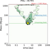 |
Fig. 23 Same as Fig. 21 but for HD 23596. There are supplementary figures in Appendix F, Fig. F.3. |
| In the text | |
|
Fig. 24 Same as Fig. 19 for α CMa B but only showing the constraints from ruwe since it was never observed with Hipparcos. Top: considering a luminous companion with both components at age ∼5 Gyr. Bottom: considering a dark companion. |
| In the text | |
|
Fig. 25 Statistics of the ratio of the single star’s UWE over the u0 published for all sources with G<16. Sources are separated into 5p and 6p datasets. |
| In the text | |
|
Fig. 26 GaiaPMEX constraints on mass and sma of a candidate companion around β Pictoris. Same caption as Fig. 19. The yellow and pink dots show the properties of the known exoplanet companions b & c in this system, with smab=9.8 ± 0.4 au and mb=10−11 MJ, and sma smac=2.7 ± 0.02 au and Mc=7.8 ± 0.4 MJ (Lagrange et al. 2020). |
| In the text | |
|
Fig. 27 Theoretical detection rates with respect to M* and the parallax. We varied the mass and the sma of the companion according to the column and row labels. White regions show the M* and the parallax for which the probability of companion detection is less than 10%; darker green regions show a probability of detection of >20%,>50% and >99%. The dashed lines show the M*-parallax relations at the limiting magnitudes of G=3 and G=16 derived from Pecaut & Mamajek (2013) tables. Similar figures are obtained considering only ruwe or PMa in Appendix G, in respectively Fig. G.1 and G.2. |
| In the text | |
|
Fig. 28 Theoretical Gaia detection rates of companions with a given mass and sma around GJ 832 as permitted by allowing a detection with PMa ∪ UEVA. White regions show the mass and sma for which the probability of detection of the companion is less than 10%; dark green regions show a probability of detection >99%; light green regions have intermediate probabilities. Individual maps for UEVA and PMa are shown in Fig. G.3. |
| In the text | |
|
Fig. C.1 Simulation of the IPD fit of a 2D Gaussian PSF on a wideorbit binary with separation of ∼200 mas and a flux ratio of 0.42. |
| In the text | |
|
Fig. C.2 Photocenter centroid variations RSE with respect to binary separation and flux ratio delineated with white contours. The red contours delineate the GOF amplitude (at levels 0.1 and 1) and the cyan contours delineate the 2 and 98% levels of the IPD_frac_multi_peak. The white hatched region shows, as discussed in the text, where the RMS of the Δη residuals could be larger than 0.1 mas, while outside this region it is always <0.1 mas. |
| In the text | |
|
Fig. D.1 Distribution of |
| In the text | |
Current usage metrics show cumulative count of Article Views (full-text article views including HTML views, PDF and ePub downloads, according to the available data) and Abstracts Views on Vision4Press platform.
Data correspond to usage on the plateform after 2015. The current usage metrics is available 48-96 hours after online publication and is updated daily on week days.
Initial download of the metrics may take a while.